Partially twisted boundary conditions for scalar mesons

Abstract:

The possibility of imposing partially twisted boundary conditions in the lattice study of the resonance states is investigated by using the effective field theory (EFT) methods. In particular, it is demonstrated that – in certain cases – it is possible to use partial twisting even in the presence of the quark annihilation diagrams. This talk is mainly based on our recent work [1], which provides substantially more details and discussion.

1 Introduction

Recently, it has been argued that the use of twisted boundary conditions [2, 3, 4] may prove useful for the extraction of the parameters of the resonances from the lattice QCD data [5, 6, 7]. In particular, this is the case when the resonances in the infinite volume are located close to the thresholds, so that, in a finite volume, one encounters a difficulty in separating these two effects in the measured spectrum. It has been explicitly demonstrated that, using twisted boundary conditions, it is possible to move threshold away from the resonance pole position. As a result, the accuracy of the extracted pole position increases dramatically [6, 7].

It should be pointed out that, imposing twisted boundary conditions on the quark fields implies, in general, calculating gauge configurations anew. For this reason, the simulations with the so-called “fully twisted” quarks are prohibitively expensive. A much cheaper solution that goes under the name of “partial twisting,” uses the same gauge configurations but twisted valence quarks in the propagators. It is clear that fully and partially twisted theories differ in a finite volume. Hence, it is legitimate to ask, whether the spectrum of the partially-twisted theory can be still used for the calculation of the physical observables.

There are the situations, when the use of the partially twisted boundary conditions can be rigorously justified (see, e.g., Refs. [3, 4]). In particular, these are the situations where the so-called annihilation diagrams of the type shown in Fig. 1 are absent. In this case, it can be proven that the potential that describes interactions in the system of two hadrons is the same in the infinite and in a finite volume, up to the exponentially suppressed terms. Consequently, the spectrum in the partially twisted case can be analyzed by using the Lüscher equation [8] which is derived in the fully twisted theory – the differences will be exponentially suppressed in a large volume.

One may easily see what goes different when the annihilation diagrams like the one shown in Fig. 1 are present. In the EFT language, the quark diagram shown in this figure corresponds to the intermediate state of two fictitious mesons consisting from one valence quark and one sea antiquark (or vice versa). The threshold of this diagram coincides with the elastic threshold – consequently, the finite-volume effects in such diagrams are only power-law suppressed and can not be neglected. On the other hand, including such intermediate states in the Lüscher equation explicitly will necessarily lead to a different equation, since the boundary conditions imposed on the fictitious mesons differ from the ones imposed on the usual ones (because the boundary conditions on the valence and sea quarks differ). Consequently, one arrives at the conclusion that, in the presence of the annihilation diagrams, the equivalence of partial and full twisting can not be proven, so one either uses full twisting or gives it up.

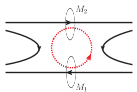
Figure 1: An example of an annihilation diagram in meson-meson scattering. The full and dashed lines denote valence and sea quarks, respectively. The intermediate state for this diagram consists of two mesons $M_{1}$ and $M_{2}$ with one valence and one sea quark.

We consider such a conclusion premature, for the following reason. As it can be seen from the discussion above, the Lüscher equation will indeed have to get modified in the presence of annihilation diagrams. However, such a modification proceeds in a well-defined manner: only two-particle intermediate states feel twisting, whereas the interaction potential between various hadron pairs stays the same in the finite volume. So, the derivation of the modified Lüscher equation is a straightforward task. A non-trivial part of the problem consists in answering the question, whether the modified Lüscher equation enables one to extract information about the physical sector of the theory (i.e., the sector with only valence quarks). If this is the case, the use of partial twisting can be still justified, even in the presence of annihilation diagrams.

In this work, we concentrate on a particular example, namely, the scalar resonance $a_{0}(980)$ with a full isospin $I=1$ and provide a complete solution of the problem in question. From this example it becomes crystal clear, how the method would work in a general case.

2 Symmetries of the hadronic potential

A straightforward way to derive Lüscher equation is to use EFT methods (see, e.g., Refs. [9, 10]). It should be stressed that, in our case, we speak of two effective theories, namely, of the partially twisted Chiral Perturbation Theory (ChPT) which is eventually matched to the non-relativistic EFT. The finite-volume spectrum of the latter theory is described by the Lüscher equation which we are aimed at to derive.

In order to arrive at the partially twisted ChPT, a standard procedure can be used (here we mainly follow Ref. [11]). The fermion sector of QCD is enlarged by introducing the so-called valence, sea and ghost (commuting) quarks:

$$\bar{\psi}(\not\!D+m)\psi\rightarrow\bar{\psi}_{\sf v}(\not\!D+m_{\sf val})\psi_{\sf v}+\bar{\psi}_{\sf s}(\not\!D+m_{\sf sea})\psi_{\sf s}+\bar{\psi}_{\sf g}(\not\!D+m_{\sf gh})\psi_{\sf g}\,,$$ (1)

where $m_{\sf val}$, $m_{\sf sea}$, $m_{\sf gh}$ are valence, sea, ghost quark mass matrices. We take them all equal (unlike the partially quenched case). However, the $SU(3)$ symmetry is not assumed, $m_{u}=m_{d}\neq m_{s}$ in all sectors. Partially twisted boundary conditions correspond to imposing twisted boundary conditions on the valence and ghost quarks and periodic boundary conditions on the sea quarks.

In the chiral limit, the infinite-volume theory is invariant under the graded symmetry group $SU(2N|N)_{L}\times SU(2N|N)_{R}\times U(1)_{V}$, where $N=3$ is the number of light flavors. The low-energy effective Lagrangian, corresponding to the case of partially twisted boundary conditions, contains the matrix $U=\exp\{i\sqrt{2}\Phi/F\}$ of the pseudo-Goldstone fields $\Phi$, which transforms under this group as

$$U\to LUR^{\dagger}\,,\quad\quad L,R\in SU(2N|N)\,.$$ (2)

The Hermitian matrix $\Phi$ has the following representation

$$\Phi=\pmatrix{M_{\sf vv}&M_{\sf sv}^{\dagger}&M_{\sf gv}^{\dagger}\cr M_{\sf sv}&M_{\sf ss}&M_{\sf gs}^{\dagger}\cr M_{\sf gv}&M_{\sf gs}&M_{\sf gg}}\,.$$ (3)

Here, each of the entries is itself a $N\times N$ matrix in flavor space, containing meson fields built up from certain quark species (e.g., from valence quark and valence antiquark, from sea quark and ghost antiquark, and so on). The fields $M_{\sf gv}$ and $M_{\sf gs}$ are anti-commuting pseudoscalar fields (ghost mesons). Further, the matrix $\Phi$ obeys the condition $\mbox{str}\,\Phi=\mbox{tr}\,(M_{\sf vv}+M_{\sf ss}-M_{\sf gg})=0\,,$ where “str” stands for the supertrace.

The effective chiral Lagrangian takes the form

$${\cal L}=\frac{F_{0}^{2}}{4}\mbox{str}\,(\partial_{\mu}U\partial^{\mu}U^{\dagger})-\frac{F_{0}^{2}}{4}\,\mbox{str}(\chi U+U\chi^{\dagger})+\mbox{higher-order terms,}$$ (4)

where $\chi=2mB_{0}$ is proportional to the quark mass matrix.

In the infinite volume, the above theory is completely equivalent to ordinary Chiral Perturbation Theory (ChPT), since the masses of the quarks of all species are set equal. In a finite volume, the difference arises due to the different boundary conditions, set on the different meson fields. These boundary conditions are uniquely determined by the boundary conditions imposed on the constituents.

Consider now the S-wave scattering of two pseudoscalar mesons in the channel with the total isospin $I=1$. This is necessarily a coupled-channel problem, with the two-particle channels containing mesons from all sectors. These channels for $I=I_{3}=1$ are listed in Table 1.

$$\begin{array}[]{|l|l|l|}\hline\cr\hline\cr\mbox{Index}&\mbox{Channel}&\mbox{Quark content}\\ \hline\cr 1&|\pi^{+}_{\sf vv}\eta_{\sf vv}\rangle&-\frac{1}{\sqrt{6}}\,|(u_{\sf v}\bar{d}_{\sf v})(u_{\sf v}\bar{u}_{\sf v}+d_{\sf v}\bar{d}_{\sf v}-2s_{\sf v}\bar{s}_{\sf v})\rangle\\ 2&|\pi^{+}_{\sf vv}\eta^{\prime}_{\sf vv}\rangle&-\frac{1}{\sqrt{3}}\,|(u_{\sf v}\bar{d}_{\sf v})(u_{\sf v}\bar{u}_{\sf v}+d_{\sf v}\bar{d}_{\sf v}+s_{\sf v}\bar{s}_{\sf v})\rangle\\ 3&|\pi^{+}_{\sf vv}\eta_{\sf ss}\rangle&-\frac{1}{\sqrt{6}}\,|(u_{\sf v}\bar{d}_{\sf v})(u_{\sf s}\bar{u}_{\sf s}+d_{\sf s}\bar{d}_{\sf s}-2s_{\sf s}\bar{s}_{\sf s})\rangle\\ 4&|\pi^{+}_{\sf vv}\eta^{\prime}_{\sf ss}\rangle&-\frac{1}{\sqrt{3}}\,|(u_{\sf v}\bar{d}_{\sf v})(u_{\sf s}\bar{u}_{\sf s}+d_{\sf s}\bar{d}_{\sf s}+s_{\sf s}\bar{s}_{\sf s})\rangle\\ 5&|\pi^{+}_{\sf vv}\eta_{\sf gg}\rangle&-\frac{1}{\sqrt{6}}\,|(u_{\sf v}\bar{d}_{\sf v})(u_{\sf g}\bar{u}_{\sf g}+d_{\sf g}\bar{d}_{\sf g}-2s_{\sf g}\bar{s}_{\sf g})\rangle\\ 6&|\pi^{+}_{\sf vv}\eta^{\prime}_{\sf gg}\rangle&-\frac{1}{\sqrt{3}}\,|(u_{\sf v}\bar{d}_{\sf v})(u_{\sf g}\bar{u}_{\sf g}+d_{\sf g}\bar{d}_{\sf g}+s_{\sf g}\bar{s}_{\sf g})\rangle\\ 7&|K^{+}_{\sf vv}\bar{K}^{0}_{\sf vv}\rangle&|(u_{\sf v}\bar{s}_{\sf v})(s_{\sf v}\bar{d}_{\sf v})\rangle\\ 8&|K^{+}_{\sf vs}\bar{K}^{0}_{\sf vs}\rangle&|(u_{\sf v}\bar{s}_{\sf s})(s_{\sf s}\bar{d}_{\sf v})\rangle\\ 9&|K^{+}_{\sf vg}\bar{K}^{0}_{\sf vg}\rangle&|(u_{\sf v}\bar{s}_{\sf g})(s_{\sf g}\bar{d}_{\sf v})\rangle\\ 10&|\pi^{+}_{\sf vs}\pi^{0}_{\sf vs}\rangle&\frac{1}{2}(-(u_{\sf v}\bar{d}_{\sf s})(u_{\sf s}\bar{u}_{\sf v}-d_{\sf s}\bar{d}_{\sf v})+(u_{\sf v}\bar{u}_{\sf s}-d_{\sf v}\bar{d}_{\sf s})(u_{\sf s}\bar{d}_{\sf v})\rangle\\ 11&|\pi^{+}_{\sf vg}\pi^{0}_{\sf vg}\rangle&\frac{1}{2}(-(u_{\sf v}\bar{d}_{\sf g})(u_{\sf g}\bar{u}_{\sf v}-d_{\sf g}\bar{d}_{\sf v})+(u_{\sf v}\bar{u}_{\sf g}-d_{\sf v}\bar{d}_{\sf g})(u_{\sf g}\bar{d}_{\sf v})\rangle\\ \hline\cr\hline\cr\end{array}$$

Table 1: Scattering channels for the case of $I=I_{3}=1$.

At the next step, the partially quenched ChPT is matched to the non-relativistic EFT with the same hadron spectrum. The two-particle scattering amplitude in the non-relativistic EFT obeys the coupled-channel Lippmann-Schwinger (LS) equation

$$T_{ij}=V_{ij}+\sum_{m,n=1}^{11}V_{im}G_{mn}T_{nj}\,,\quad\quad i,j=1,\cdots,11\,.$$ (6)

By using dimensional regularization, the above equation becomes an algebraic equation, where both the $T_{ij}$ and the potential $V_{ij}$ are evaluated on shell (the potential $V_{ij}$ coincides with the multichannel $K$-matrix in this formalism). The quantity $G_{ij}$ stands for the two-particle loops in the intermediate state. This quantity is not diagonal due to the mixing of the neutral states, so, in order to calculate this quantity, one has first to diagonalize it the the basis of physical neutral mesons and then use the prescriptions of the non-relativistic EFT for calculating a loop. The details can be found in Ref. [1].

The entries of $T_{ij}$ and $V_{ij}$, corresponding to the scattering fully in the valence sector, are termed as physical. The quark diagrams, describing the amplitudes in this sector, are the same as in ordinary QCD. However, $T_{ij}$ and $V_{ij}$ contain unphysical entries as well, describing the transitions between valence/sea/ghost sectors. The quark diagrams describing these transitions are, in general, different (e.g., containing only disconnected contributions). So, the question arises, whether one is able to relate the finite-volume spectrum of the theory to the physical matrix elements only.

The key property which allows one to do so is the symmetry of $T_{ij}$ and $V_{ij}$, which stems from the $SU(2N|N)_{L}\times SU(2N|N)_{R}\times U(1)_{V}$ graded symmetry of the original theory. In particular, it can be shown that the matrix elements of these matrices obey certain linear relations which reduce the number of the independent entries. As a nice check, it can be verified that, due to these constraints, the relation between the $T$- and $K$-matrix elements in the infinite volume turns out to be the same as in ordinary ChPT, without sea and ghost quarks. In fact, in the infinite volume these two theories should be exactly equivalent.

3 Derivation of the partially twisted Lüscher equation

In a finite volume, only the matrix $G$ containing two-meson loops changes $G\to G_{L}$, where the matrix elements of $G_{L}$ are linear combinations of the Lüscher zeta-functions. The potential remains the same. The spectrum is determined from the secular equation

$$\mbox{det}\,(1-VG_{L})=0\,.$$ (7)

Various scenarios of the partial twisting lead to the different modifications of $G$ and hence to the different versions of the Lüscher equation. Below, we shall consider two scenarios. The general pattern will be clear from these examples.

Scenario 1:

We impose periodic boundary conditions on the $u$-,$d$-quarks and twisted boundary conditions on the $s$-quark:

$$u({\bf x}+{\bf n}L)=u({\bf x})\,,\quad d({\bf x}+{\bf n}L)=d({\bf x})\,,\quad s({\bf x}+{\bf n}L)=e^{i\theta n}s({\bf x})\,.$$ (8)

These boundary conditions translate into the boundary conditions for the meson states. Only the boundary conditions for the kaons change:

$$K^{\pm}({\bf x}+{\bf n}L)=e^{\mp i\theta n}K^{\pm}({\bf x})\,,\quad\!\!K^{0}({\bf x}+{\bf n}L)=e^{-i\theta n}K^{0}({\bf x})\,,\quad\!\!\bar{K}^{0}({\bf x}+{\bf n}L)=e^{i\theta n}\bar{K}^{0}({\bf x})\,.$$ (9)

This means that $K$ and $\bar{K}$ mesons containing valence and ghost $s$-quarks get additional 3-momenta $\mp\theta/L$. The system stays in the CM frame. The secular equation takes the form

$$(1-V_{77}K_{L}-V_{11}E_{L}+(V_{77}V_{11}-V_{17}^{2})K_{L}E_{L})F_{L}(\theta)=0\,,$$ (10)

where $K_{L}$ and $E_{L}$ denote the $K\bar{K}$ and $\pi\eta$ loops in a finite volume in the absence of twisting

$$K_{L},E_{L}=\frac{1}{4\pi^{3/2}P_{0}L}\,Z_{00}(1;q^{2})\,,\quad\quad q=\frac{pL}{2\pi}\,,$$ (11)

$p$ is the magnitude of the relative three-momentum of a pair in the CM frame ($K\bar{K}$ or $\pi\eta$ pair, respectively), and $P_{0}$ is the total energy of a pair. The quantity $F_{L}(\theta)$ denotes a factor that depends on the unphysical entries of the matrix $V$.

As seen, owing to the symmetries of the matrix $V$, the determinant in the secular equation was split, and a piece containing only physical amplitudes, has emerged. The resulting equation is, however, not very useful because it coincides with the equation with no twisting.

As seen, the spectrum of the partially twisted equation contains more states than the fully twisted one (these are the solutions of the equation $F_{L}(\theta)=0$). Physically, these solutions are not interesting because the physical and non-physical matrix elements are intertwined here. It could be shown that, choosing particular source/sink operators, which do not have an overlap with some of the states, one may project out the physical part of the spectrum.

Scenario 2:

Here we consider twisting of the $u$-quark, leaving the $d$- and $s$-quarks to obey periodic boundary conditions. What changes here is the free Green function in a finite volume.

$$K,E\to K_{L}^{\theta},E_{L}^{\theta}=\frac{1}{4\pi^{3/2}\sqrt{s}\gamma L}\,Z_{00}^{\bf d}(1;(q^{*})^{2})\,,\quad q^{*}=\frac{p^{*}L}{2\pi}\,,\quad p^{*}=\frac{\lambda^{1/2}(s,m_{1}^{2},m_{2}^{2})}{2\sqrt{s}}\,.$$ (12)

where ${\bf d}={\bf P}L/2\pi=\theta/2\pi$, $s=P_{0}^{2}-{\bf P}^{2}$, $\gamma=P_{0}/\sqrt{s}$, the quantity $\lambda(x,y,z)$ is Mandelstam triangle function and $Z_{00}^{\bf d}(1;(q^{*})^{2})$ denotes the Lüscher zeta-function in the moving frame [12], see also Refs. [13, 14]:

$$Z_{00}^{\bf d}(1;(q^{*})^{2}) = \frac{1}{\sqrt{4\pi}}\,\sum_{{\bf r}\in P_{d}}\frac{1}{{\bf r}^{2}-(q^{*})^{2}}\,,$$

$$P_{d} = \{{\bf r}=\mathbb{R}^{3}~{}|~{}r_{\parallel}=\gamma^{-1}(n_{\parallel}-\mu_{1}|{\bf d}|),~{}{\bf r}_{\perp}={\bf n}_{\perp},~{}{\bf n}\in\mathbb{Z}^{3}\}\,,$$ (13)

where $\mu_{1}=\bigl{(}1-(m_{1}^{2}-m_{2}^{2})/s\bigr{)}/2$.

The secular equation in a finite volume takes the form

$$(1-V_{77}K_{L}^{\theta}-V_{11}E_{L}^{\theta}+(V_{77}V_{11}-V_{17}^{2})K_{L}^{\theta}E_{L}^{\theta})F^{\prime}_{L}(\theta)=0\,,$$ (14)

where $F^{\prime}_{L}(\theta)$ is another factor, depending on the unphysical entries. It is seen that the spectra in case of the partial and full twisting coincide.

4 Summary

Using the non-relativistic EFT technique in a finite volume, we have derived the Lüscher equation for the partially twisted boundary conditions for coupled-channel $\pi\eta-K\bar{K}$ scattering. Our final result is remarkably simple. If in the channel with $I=I_{3}=1$ the light quarks are subject to twisting, the partially twisted Lüscher equation is equivalent to the fully twisted one, despite the presence of annihilation diagrams. If, on the contrary, partial twisting of the strange quark is performed, the physically interesting part of the spectrum is not affected. Other scenarios are also possible and can be investigated by using the same methods.

We think that this result would be interesting for the lattice practitioners studying the properties of scalar mesons. We have shown that, instead of carrying out simulations at different volumes, as required in the Lüscher approach, one may perform relatively cheaper partially twisted simulations.

References

- [1] D. Agadjanov, U.-G. Meißner and A. Rusetsky, arXiv:1310.7183 [hep-lat].
- [2] P. F. Bedaque, Phys. Lett. B 593 (2004) 82. G. M. de Divitiis, R. Petronzio and N. Tantalo, Phys. Lett. B 595 (2004) 408. G. M. de Divitiis and N. Tantalo, arXiv:hep-lat/0409154.
- [3] C. T. Sachrajda and G. Villadoro, Phys. Lett. B 609 (2005) 73.
- [4] P. F. Bedaque and J.-W. Chen, Phys. Lett. B 616 (2005) 208.
- [5] V. Bernard, M. Lage, U.-G. Meißner and A. Rusetsky, JHEP 1101 (2011) 019.
- [6] M. Döring, U.-G. Meißner, E. Oset and A. Rusetsky, Eur. Phys. J. A 47 (2011) 139.
- [7] M. Döring, U.-G. Meißner, E. Oset and A. Rusetsky, Eur. Phys. J. A 48 (2012) 114.
- [8] M. Lüscher, Nucl. Phys. B 354 (1991) 531.
- [9] S. R. Beane, P. F. Bedaque, A. Parreno and M. J. Savage, Nucl. Phys. A 747 (2005) 55.
- [10] V. Bernard, M. Lage, U.-G. Meißner and A. Rusetsky, JHEP 0808 (2008) 024.
- [11] S. R. Sharpe and N. Shoresh, Phys. Rev. D 64 (2001) 114510.
- [12] K. Rummukainen and S. A. Gottlieb, Nucl. Phys. B 450 (1995) 397.
- [13] M. Göckeler, R. Horsley, M. Lage, U.-G. Meißner, P. E. L. Rakow, A. Rusetsky, G. Schierholz and J. M. Zanotti, Phys. Rev. D 86 (2012) 094513.
- [14] V. Bernard, D. Hoja, U.-G. Meißner and A. Rusetsky, JHEP 1209 (2012) 023.