The Plasma Simulation Code: A modern particle-in-cell code with load-balancing and GPU support

Abstract

Recent increases in supercomputing power, driven by the multi-core revolution and accelerators such as the IBM Cell processor, graphics processing units (GPUs) and Intel’s Many Integrated Core (MIC) technology have enabled kinetic simulations of plasmas at unprecedented resolutions, but changing HPC architectures also come with challenges for writing efficient numerical codes. This paper describes the Plasma Simulation Code (psc), an explicit, electromagnetic particle-in-cell code with support for different order particle shape functions. We focus on two distinguishing features of the code: patch-based load balancing using space-filling curves, and support for Nvidia GPUs, which achieves a substantial speed-up of up to more than $6\times$ on the Cray XK7 architecture compared to a CPU-only implementation.

1 Introduction

Rapidly advancing computer technology has enabled large first-principles plasma simulations in recent years. The kinetic description of plasma, the Vlasov-Maxwell system of equations, while computationally much more expensive, overcomes many limitations of fluid descriptions like magnetohydrodynamics (MHD) or extended MHD models. Fluid models describe plasma behavior at large scales very well, but approximations need to be made at small scales, which occur in magnetic reconnection and turbulence. For example, the one-fluid approximation breaks down at the ion skin depth scale $d_{i}$, electrons and ions decouple, and the magnetic field remains frozen to the electron flow. Reconnection requires breaking the frozen-in condition that occurs at electron scales, which can be represented in a fluid model in a generalized Ohm’s Law that includes electron inertia and electron pressure tensor effects. Finding appropriate closures is still an area of active research, see e.g. [1]. Kinetic particle-in-cell simulations also allow investigation of problems beyond the scope of fluid models, e.g. particle acceleration [2]. Particle-in-cell codes, while often run with modified physical parameters (e.g. reduced ion/electron mass ratio and speed of light), are now capable of simulating multi-scale problems spanning from electron through ion to global scales reaching 100’s of $d_{i}$ in two and even three dimensions. While efforts are underway to overcome some of the algorithmic limitations of explicit particle-in-cell methods (see, e.g., [3, 4]), explicit particle-in-cell methods scale efficiently to the largest supercomputers available today and are commony used to address challenging science problems.

The Plasma Simulation Code (psc) is an explicit, electromagnetic particle-in-cell code implementing similar methods as, e.g., vpic [5], osiris[6] and vorpal [7]. psc is based on H. Ruhl’s original version [8], but has been rewritten as modular code that supports flexible algorithms and data structures. Beyond its origin in the field of laser-plasma interaction, psc has been used in studies of laser-induced plasma bubbles [9, 10, 11, 12], particle acceleration [13], and closure aspects in magnetic reconnection [14].

In this paper, we will review the main underlying particle-in-cell methods, and then focus on two distinguishing features implemented in psc: Patch-based load balancing and GPU support. Patch-based dynamic load balancing addresses both performance and memory issues in simulations where many particles move between local domains. GPU support enhances performance by more than $6\times$ on the Cray XK7 architecture by making use of the Nvidia K20X GPU.

2 Particle-in-cell method

2.1 Kinetic description of plasmas

The particle-in-cell method [15, 16, 4] solves equations of motion for particles and Maxwell’s equations to find forces between those particles, which is very similar to the first-principle description of a plasma as a system of charged particles. It is, however, better understood as a numerical method to solve the Vlasov-Maxwell system of equations that describes the time evolution of the particle distribution function $f_{s}(\mathbf{x},\mathbf{p},t)$ where $s$ indicates the species:

$$\frac{\partial f_{s}}{\partial t}+\mathbf{v}\cdot\frac{\partial f_{s}}{\partial\mathbf{x}}+q_{s}(\mathbf{E}+\mathbf{v}\times\mathbf{B})\cdot\frac{\partial f_{s}}{\partial\mathbf{p}}=0$$ (1)

The electromagnetic fields $\mathbf{E}$ and $\mathbf{B}$ are self-consistently evolved using Maxwell’s equations:

$$\nabla\cdot\mathbf{E} = \frac{\rho}{\epsilon_{0}}$$ (2)

$$\nabla\cdot\mathbf{B} = 0$$ (3)

$$\frac{\partial\mathbf{E}}{\partial t} = c^{2}\nabla\times\mathbf{B}-\frac{\mathbf{j}}{\epsilon_{0}}$$ (4)

$$\frac{\partial\mathbf{B}}{\partial t} = -\nabla\times\mathbf{E}$$ (5)

where charge density $\rho$ and current density $\mathbf{j}$ are obtained from the particle distribution functions:

$$\rho = \sum_{s}q_{s}\int f_{s}(\mathbf{x},\mathbf{p},t)\,d^{3}p$$ (6)

$$\mathbf{j} = \sum_{s}q_{s}\int\mathbf{v}f_{s}(\mathbf{x},\mathbf{p},t)\,d^{3}p$$ (7)

The divergence equations (2), (3) in Maxwell’s equations can be considered as initial conditions. If they are satisified at some initial time, it is easy to show from Ampére’s Law (4) and Faraday’s Law (5) that they will remain satisifed at all times provided that the charge continuity equation also holds:

$$\partial_{t}\rho+\nabla\cdot\mathbf{j}=0.$$ (8)

2.1.1 Particle-in-Cell method

The particle-in-cell method approximates the distribution function $f_{s}$ by representing it using quasi-particles with finite extent in configuration space:

$$f_{s}(\mathbf{x},\mathbf{p},t)=\sum_{i=1}^{N_{s}}N^{s}_{i}\phi(\mathbf{x}-\mathbf{x}_{i}^{s}(t))\,\delta^{3}(\mathbf{p}-\mathbf{p}_{i}^{s}(t))$$ (9)

Using the $\delta$-function in velocity space ensures that the spatial extent of each quasi-particle remains constant in time.

The selection of the shape function $\phi$ determines properties of the numerical method. In general, the 3-d shape function is chosen to be the tensor product of 1-d shape functions in each coordinate direction; normalized, symmetric shape functions with compact support are used. Equations of motions for the quasi-particles can then be derived by taking moments of the Vlasov equation:

$$\frac{dN^{s}_{i}}{dt}=0\;,\;\;\frac{d\mathbf{x}_{i}^{s}}{dt}=\mathbf{v}_{i}^{s}\;,\;\;\frac{d\mathbf{p}_{i}^{s}}{dt}=q_{s}(\mathbf{E}_{i}+\mathbf{v}_{i}^{s}\times\mathbf{B}_{i})$$ (10)

The first equation expresses that the number of actual particles $N^{s}_{i}$ that each quasi-particle $i$ of species $s$ represents remains constant. The other two equations are the usual equations of motion for a point particle with the modification that the electromagnetic fields $\mathbf{E}_{i},\mathbf{B}_{i}$ acting on the particle are given by

$$\mathbf{E}_{i}=\int\mathbf{E}\,\phi(\mathbf{x}-\mathbf{x}_{i}^{s})\,d^{3}x\;,\;\;\mathbf{B}_{i}=\int\mathbf{B}\,\phi(\mathbf{x}-\mathbf{x}_{i}^{s})\,d^{3}x$$ (11)

which means that the electromagnetic fields are averaged over the extent of the particle.

Using finite-size quasi-particles is the main advantage of the particle-in-cell method. It is computationally cheaper, since it allows one to solve the field equations on a mesh, rather than directly calculating the interaction of each particle with all others. Particle-in-cell scales linearly in the number of particles $N$, as opposed to exact interaction approach that scales like $\mathcal{O}(N^{2})$ (though this can be improved to $\mathcal{O}(N\log N)$ by fast multipole methods [17]). More importantly, even with today’s very powerful computers it is not possible to simulate as many particles as comprise real plasmas of interest, and it will remain unfeasible for the foreseeable future. In lowering the number of particles to a number that is possible to simulate one must be careful to not change the nature of the plasma. Plasmas are traditionally weakly coupled, ie. the interaction between particles is dominated by collective behavior rather than individual particle-particle forces. The particle-in-cell method reduces the occurence of strong particle-particle interactions because particles are now of finite extent, which means that their interaction potential weakens when two particles approach closer than their spatial size, while still representing the long-range interactions faithfully.

2.2 FDTD method for solving Maxwell’s equations

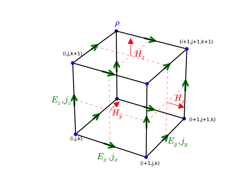
Figure 1: The staggered Yee grid unit cell. Depicted are the locations of magnetic fields on face centers (red), eletric fields and current density (green), and charge density (blue)

Figure 2: Leap-frog time integration in the PIC method. Blue quantities represent electromagnetic field quantities and their update scheme. Red quantities are quasi-particle positions and momenta, also staggered in time. Interaction occurs by using the EM fields to find the Lorentz force on particles (black) and by using particle motion to find current density that feeds back into Maxwell’s equations (green).

The finite-difference time domain (FDTD) method has a long history of being used for computationally solving Maxwell’s equations [18]. The FDTD method has the desirable feature of satisfying some conservation properties of the underlying continuum equations in the discrete. It employs the staggered Yee grid, as shown in Fig. 2, to represent magnetic fields on faces, electric fields and current densities on edges, and charge densities on corners of the computational mesh.

We define the following discrete curl operators:

$$(\nabla^{+}\times\mathbf{E})_{x,i,j+1/2,k+1/2} = \frac{E_{z,i,j+1,k+1/2}-E_{z,i,j,k+1/2}}{\Delta y}-\frac{E_{y,i,j+1/2,k+1}-E_{y,i,j+1/2,k}}{\Delta z}$$ (12)

$$(\nabla^{-}\times\mathbf{B})_{x,i+1/2,j,k} = \frac{B_{z,i+1/2,j+1/2,k}-B_{z,i+1/2,j-1/2,k}}{\Delta y}-\frac{B_{y,i+1/2,j,k+1/2}-B_{y,i+1/2,j,k-1/2}}{\Delta z}$$ (13)

where the $y$ and $z$ components are obtained by cyclic permutation.

We also define the following discrete divergence operators:

$$(\nabla^{+}\cdot\mathbf{B})_{i+1/2,j+1/2,k+1/2} = \frac{B_{x,i+1,j+1/2,k+1/2}-B_{x,i,j+1/2,k+1/2}}{\Delta x}+\frac{B_{y,i+1/2,j+1,k+1/2}-B_{y,i+1/2,j,k+1/2}}{\Delta y}+$$ (15)

$$\frac{B_{z,i+1/2,j+1/2,k+1}-B_{z,i+1/2,j+1/2,k}}{\Delta z}$$

$$(\nabla^{-}\cdot\mathbf{E})_{i,j,k} = \frac{E_{x,i+1/2,j,k}-E_{x,i-1/2,j,k}}{\Delta x}+\frac{E_{y,i,j+1/2,k}-E_{y,i,j-1/2,k}}{\Delta y}+\frac{E_{z,i,j,k+1/2}-E_{z,i,j,k-1/2}}{\Delta z}$$ (16)

Maxwell’s equations are discretized using these operators, and we employ a leap-frog scheme staggered in time (see also Fig. 2):

$$\frac{\mathbf{E}^{n+1/2}_{ijk}-\mathbf{E}^{n-1/2}_{ijk}}{\Delta t} = c^{2}\nabla^{-}\times\mathbf{B}^{n}_{ijk}-\frac{\mathbf{j}^{n}_{ijk}}{\epsilon_{0}}$$ (17)

$$\frac{\mathbf{B}^{n+1}_{ijk}-\mathbf{B}^{n}_{ijk}}{\Delta t} = -\nabla^{+}\times\mathbf{E}^{n+1/2}_{ijk}$$ (18)

where

$$\mathbf{E}_{ijk} = \left(E_{x,i+1/2,j,k},E_{y,i,j+1/2,k},E_{z,i,j,k+1/2}\right)$$ (20)

$$\mathbf{B}_{ijk} = \left(B_{x,i,j+1/2,k+1/2},B_{y,i+1/2,j,k+1/2},B_{z,i+1/2,j+1/2,k}\right)$$ (21)

It is easy to show that the discrete operators satisfy

$$\nabla^{+}\cdot\nabla^{+}\times=0\;,\;\;\nabla^{-}\cdot\nabla^{-}\times=0$$ (23)

and hence, as in the continuum, the discretized divergence equations remain satisfied to round-off error at all times,

$$(\nabla^{-}\cdot\mathbf{E})_{ijk}=\frac{\rho_{ijk}}{\epsilon_{0}}\;,\;\;(\nabla^{+}\cdot\mathbf{B})_{i+1/2,j+1/2,k+1/2}=0$$ (24)

provided that the charge continuity equation is also discretely satisfied:

$$\frac{\rho^{n+1/2}_{ijk}-\rho^{n-1/2}_{ijk}}{\Delta t}+(\nabla^{-}\cdot\mathbf{j})_{ijk}=0$$ (25)

The FDTD method also satisifies a discrete version of Poynting’s Theorem; however, when used in the context of a PIC method energy is generally not exactly conserved because $\mathbf{j}\cdot\mathbf{E}$ is discretized differently in the Maxwell solver compared to the particle advance.

2.3 Time integration of the quasi-particle equations of motion

We use a standard leap-frog method to advance quasi-particles in time, see also Fig. 2.

$$\frac{\mathbf{x}_{i}^{n+1/2}-\mathbf{x}_{i}^{n-1/2}}{\Delta t} = \mathbf{v}_{i}^{n}$$ (26)

$$\frac{\mathbf{p}_{i}^{n+1}-\mathbf{p}_{i}^{n}}{\Delta t} = q_{s}\left(\mathbf{E}_{i}^{n+1/2}+\mathbf{v}_{i}^{n+1/2}\times\mathbf{B}_{i}^{n+1/2}\right)$$ (27)

where $\mathbf{v}_{i}^{n}=\mathbf{p}_{i}^{n}/(m_{s}\gamma_{i}^{n})$. We follow Boris [19] in choosing

$$\mathbf{v}_{i}^{n+1/2}=\frac{\mathbf{p}_{i}^{n}+\mathbf{p}_{i}^{n+1}}{2m_{s}\gamma_{i}^{n+1/2}}$$ (28)

and splitting the momentum update into a half step acceleration by $\mathbf{E}$, a rotation by $\mathbf{B}$, and another half step acceleration by $\mathbf{E}$.

The shape functions used in the psc code are standard B-splines [4, 15]. The code currently supports both 1st and 2nd order interpolation by employing the flat-top $b_{0}(\xi)$ B-spline and the triangular-shaped $b_{1}(\xi)$ B-spline. $b_{0}(\xi)$ is defined as

$$b_{0}(\xi)=\left\{\begin{array}[]{ll}1&\textrm{if $|\xi|<1/2$}\\ 0&\textrm{otherwise}\end{array}\right.$$ (29)

Successive B-splines are defined recursively by folding the previous B-spline with $b_{0}$:

$$b_{n+1}=\int_{-\infty}^{\infty}b_{0}(\xi-\xi^{\prime})b_{n}(\xi-\xi^{\prime})\,d\xi^{\prime}$$ (30)

In particular, the psc code uses $b_{1}$ and $b_{2}$:

$$b_{1}(\xi)=\left\{\begin{array}[]{ll}1+\xi&\textrm{if $-1\leq\xi\leq 0$}\\ 1-\xi&\textrm{if $\;\;0\leq\xi\leq 1$}\\ 0&\textrm{otherwise}\end{array}\right.\qquad b_{2}(\xi)=\left\{\begin{array}[]{ll}\frac{1}{2}\left(\frac{3}{2}+\xi\right)^{2}&\textrm{if $-\frac{3}{2}\leq\xi\leq-\frac{1}{2}$}\\ \frac{3}{4}-\xi^{2}&\textrm{if $-\frac{1}{2}\leq\xi\leq\frac{1}{2}$}\\ \frac{1}{2}\left(\frac{3}{2}-\xi\right)^{2}&\textrm{if $\;\;\frac{1}{2}\leq\xi\leq\frac{3}{2}$}\\ 0&\textrm{otherwise}\end{array}\right.$$ (31)

B-splines are commonly used in PIC codes because of their simplicity and compact support. Also, when assuming that the electromagnetic fields are piecewise constant about their staggered grid locations the integrals in Eq. 11 are conveniently evaluated and found to be B-splines themselves, of order one higher than the shape function itself. Hence the psc code uses B-splines of order 1 and 2 to interpolate the electromagnetic fields to the quasi-particle position.

2.4 Time integration

The particle-in-cell method advances both electromagnetic fields and quasi-particles self-consistently. The time integration scheme used in psc is sketched out in Fig. 2. The figure shows the FDTD scheme (blue), and particle integrator (red), and also their interactions: To update the momentum, the electric and magnetic fields are needed to find the force on a given quasi-particle (black arrows). $\mathbf{E}^{n+1/2}$ exists at the proper centered time to do so, while $\mathbf{B}^{n+1/2}$ is in principle found by averaging $\mathbf{B}^{n}$ and $\mathbf{B}^{n+1}$; however, in practice, we rather split the $\mathbf{B}^{n}\rightarrow\mathbf{B}^{n+1}$ update into two half steps.

Particle motion feeds back into Maxwell’s equations by providing the source term $\mathbf{j}^{n}$. The current density is computed from the particles to exactly satisfy the discrete charge continuity equation, which requires knowing particle positions at the naturally existing $\mathbf{x}^{n-1/2}$ and $\mathbf{x}^{n+1/2}$, and is fed back into Maxwell’s equations (green arrows).

psc uses two methods to satisfy charge continuity: For 1st-order particles we use the scheme by Villasenor-Buneman [20], while for 2nd-order particles we follow the method by Esirkepov [21]. psc also implements some alternating-order interpolation schemes from [22] for improved energy conservation. For a discussion of conservation properties of particle-in-cell codes, see also [23].

We find that single precision simulations that run for a very large number of steps accumlate round-off errors that lead to growing deviations from the discrete Gauss’s Law. psc implements the iterative method by Marder [24] to dissipate violations of Gauss’s Law.

The psc code supports a number of additional features, including an approximate Coulomb collision operator (see [10]), periodic, reflecting conducting wall, and open boundary conditions (as in [25]), moving window and boost frame, which are not addressed in detail here.

3 Overview of the PSC code

The Plasma Simulation Code (psc) presented in this paper is based on the original Fortran code by H. Ruhl [8], but it has been largely rewritten. The original Fortran computational kernels (particle advance, FDTD Maxwell solver) are still available as modules, but the code’s overall framework is now written in the C programming language.

The structure of the code is based on libmrc, a parallel object model and library that forms the basis of a number of simulation codes maintained by the author, including the Magnetic Reconnection Code (mrcv3) [26, 27, 28] and J. Raeder’s global magnetosphere code openggcm [29, 30]. We consider libmrc to be a library rather than a framework, because it consolidates commonly used computational techniques in order to avoid reimplementing and maintaining common tasks like domain decomposition and I/O in individual codes. It is designed so that only selected parts of it can be used (e.g., filling of ghost points) in an otherwise legacy code without requiring large changes to the structure of the code overall.

libmrc is written in C, but supports Fortran-order multidimensional arrays to enable easy interfacing with existing Fortran code. Its basis is an object model that is quite similar to the one used in PETSc [31, 32, 33] – and libmrc can optionally interface with PETSc to provide linear and nonlinear solvers, etc., though this feature is not used in the psc code. Objects can be instantiated in parallel, i.e. they have an MPI communicator associated with them. Objects instantiate a given class, which essentially defines an interface. In the PIC context, for example, this may be a field pusher which provides two methods to update electric and magnetic fields, respectively. There may be more than one implementation for a given class, which we call “subclasses” or “types”. In the example of the field pusher, this may be a single precision or double precision implementation of the FDTD method, or it could potentially encompass methods other than FDTD. In the case of the particle pusher, there are types for first and second order particle shapes, or a particle pusher that runs on GPUs. Like PETSc objects, the type of a given object can be set at run time – potentially from a command line option, which allows the user to easily switch out modules in a given run.

The libmrc library provides a number of classes for common computational tasks, e.g. a parallel multi-dimensional field type which is distributed amongst MPI processes and associated coordinates. It handles parallel I/O; currently implemented options include the simple “one file per MPI process” approach as well as parallel XDMF/HDF5 [34] output using a subset of I/O writer nodes. As we will explain in more detail in the load balancing section, libmrc fields can be decomposed into many “patches”, where a given MPI process may handle more than one patch – the very same interface is used to support block-structured adaptive mesh refinement, where again a given process handles multiple patches which are possibly at different levels of resolution. libmrc objects maintain explicit information about their own state, e.g. an object knows about member variables that are parameters, so these can be automatically parsed from the command line. This also simplifies checkpoint / restart: Every object knows how to write itself to disk, and how to restore itself, which means that writing a checkpoint just consists of walking down the hierarchy of objects asking each object to checkpoint itself.

The psc code uses libmrc objects extensively: There are objects for all computational kernels (particles, fields), particle boundary exchange / filling ghost points, outputting fields and particles, etc. All these objects are contained within one psc object that represents the overall simulation. To implement a particular case one “derives” from the psc object, i.e. one implements a particular subclass. In this subclass one can overwrite various methods as needed – the create() methods to set defaults for domain size, resolution, normalization, particles species, etc., the init_fields() method to set initial conditions, and similarly an init_npt() method to set the initial condition for particles.

The aforementioned objects are primarily used to select particular algorithms, i.e. a second or first order particle pusher has little or no state associated with it but rather just implements a different computational algorithm. The simulation state is maintained in two additional objects: psc_fields and psc_particles, which are the large distributed arrays that represent the field and particle state. Those objects themselves may actually be implemented as rather different data structures: The particle data may be a simple array of struct in double precision living in CPU memory, but it can also be a more complicated struct of arrays of small vectors in GPU memory in single precision, just by selecting its subclass to be either “double” or “cuda”.

The flexibility of supporting multiple data layouts is crucial to supporting both CPUs and GPUs in one code, but it also presents a significant challenge in implementing the algorithms that actually work on that data. For example, for obvious reasons a CPU particle pusher will not work when the particle data passed to it actually lives in GPU memory and/or is in the wrong layout. In traditional object oriented programming the solution to this is to not access data directly, but to virtualize it through methods of the particle object. However, for a high-performance code it is not acceptable to abstract all accesses through virtual (indirect) method calls because of the performance penalties incurred.

Another solution is to only support a matching set of modules – double precision CPU particle pusher with double precision CPU particles and double precision CPU fields. However, this means one essentially has to rewrite the entire code to support, e.g., a GPU implementation, which is a large effort and can easily lead to maintenance problems as CPU and GPU capabilities of the code can diverge.

psc resolves this problem differently: A particle pusher expecting double precision particles on the CPU needs to wrap its computations inside a pair of particles_get_as("double") and particles_put_as() calls. The particle data structure returned from the get_as() call is guaranteed to be of the requested type, so the actual computation can be performed by directly accessing the known data structures without any performance penalties. Behind the scenes, the get_as() and put_as() calls perform conversion of the data structures if needed – if the particle data was actually stored as single precision it would be converted to double precision first, and the result will later (in put_as()) be converted back. If the particle data was already of the type requested, get_as() and put_as() perform no actual work.

The main advantage to this approach is that it is now possible to implement new computational kernels one at a time, while keeping the overall code functional. There is of course a performance penalty for the data layout conversion, and it is typically severe enough that, for production runs, one wants to select a matching set of modules, e.g. particle and field data, particle pusher, and field pusher all of the “cuda” type for running on the GPU. Still, the main computational kernels are only a small fraction of the code overall, and other functionality like I/O and analysis often occur rarely enough that for those routines the conversion penalty is small, so it is not necessary to rewrite them for the new data types.

It should be noted that while a particle pusher on the CPU looks quite different from that on the GPU (so there is only limited room to share code), a second order pusher on the CPU working on single precision data is very similar to the same in double precision, so in this case we use a shared source file that gets compiled into a single and a double version by using the C preprocessor. While we end up with two distinct subclasses (“2nd_single” and “2nd_double”), we avoid unnecessary code duplication.

As mentioned before, output is typically written as XDMF/HDF5, which allows directly visualizing the data with Paraview, though we typically use custom scripts in Python or Matlab to downscale the resolution and perform specific analyses.

4 Parallelization and load balancing

4.1 Parallelizing particle-in-cell simulations

Figure 3: Initial condition for a laser-generated plasma bubble simulation. Shown are the plasma density (green) and the uniform domain decomposition of the computational domain into $100\times 80$ patches.

Due to their dual nature, particle-in-cell simulations are inherently more difficult to parallelize than either purely mesh-based or purely particle-based algorithms. For both mesh-based and particle-based methods a data parallel approach is fairly straightforward, but the two-way interactions between fields and particles in the PIC method requires an approach that takes these interactions into account. In the following, we consider parallelization on a distributed memory machine using the message passing paradigm. Virtually all large supercomputers follow this paradigm as the coarse level of parallelism. Lower levels, like shared memory parallelization on a node or small vector instructions on a core, need to also be used but will be discussed later.

In a mesh-based simulation the typical approach to parallelization is domain decomposition: the spatial domain is subdivided into smaller subdomains, each subdomain is assigned to a different processing unit and processed separately. This works well if the computation is local in space, e.g. a stencil computation with a small stencil, as is the case for the FDTD scheme employed in psc. Near the subdomain boundaries some data points from neighboring subdomains are required to update the local domain; these need to be communicated by message passing and are typically handled by a layer of ghost cells (also called halo regions). Domain decomposition for structured grids is a well established method and scales well as long as the boundary-related work remains small compared to the bulk computation, i.e. as long as the surface-to-volume ratio remains small.

In purely particle-based simulations, distributing particles in a data-parallel way is fundamentally quite simple, by just assigning subsets of particles to processors; however, interactions between particles will need to be taken into account and depending on their nature can make it rather challenging to find a parallel decomposition that still allows for efficient computation of those interactions, e.g., in the case of the fast multipole method [35].

For particle-in-cell simulations, interactions happen between particles and fields but not between particles and particles directly. An exception is the implementation of a collision operator, which approximates interactions of close-by particles by randomly picking representative particle pairs that are in close spatial vicinity.

Performance of particle-in-cell simulations is normally dominated by particle-related computational kernels rather than field computations, simply due to the fact that there are typically 100 or more particles per grid cell. Although, this assumption is not always true, in particular in a local sense. Simulations of laser-plasma interaction may have a significant fraction of the simulation that represent light waves in vacuum, and simulations of magnetic reconnection like-wise may have spatial regions at low density that are represented by just a few particles per cell.

Given these constraints, two approaches have been popular to parallelize particle-in-cell simulations on distributed memory machines:

(1) Distribute particles equally between processing units and redundantly keep copies of the fields on all processing units.

(2) Use a spatial decomposition of the domain and distribute particles according to which subdomain they are located in, so that particles and fields are maintained together on the same processing unit.

The main advantage to method (1) is its simplicity. Particles can be pushed independently of where they are located in the domain since all fields are available. As they move, current or charge density is deposited into the corresponding global fields. There are no load balancing issues – particles are distributed to processes equally in the beginning, and since they never move between processes this balance is maintained. The main drawback in this scheme is that the source terms for Maxwell’s equations need to include contributions of all particles, so a global reduction for each global grid point is required at each time step. Maxwell’s equations can be solved on one processor and the resulting fields broadcast to all processes, or the aggregated source field(s) can be broadcast and the computation performed redundantly on all processing units. The large, global reductions severely limit the parallel scalability and limit the applicability of the scheme to at most 100s of cores.

Method (2) overcomes the scalability limitations of the previous scheme and is the approach used in state-of-the-art codes like vpic [5], osiris [6], and psc. Its implementation is more involved – particles will leave the local subdomain and need to be communicated to their new home. The field integration is performed locally on the subdomain and is therefore scalable. Both field integration and particles moving near boundaries require appropriate layers of ghost cells, and near subdomain boundaries proper care needs to be taken to correctly find contributions to the current density from particles in a neighboring subdomain, whose shape functions extend into the local domain.

Relativistic, explicit, electromagnetic particle-in-cell codes that follow the latter parallelization approach generally show excellent parallel scalability. Recently, osiris [6] has shown to scale to the full machine on NSF’s Bluewaters Cray supercomputer. Fundamentally, this is easily explained by the underlying physics: Both particles and waves can propagate at most at the speed of light – since the time step is constrained by the CFL condition, information is guaranteed to propagate at most one grid cell per time step. Therefore interactions in the interior of the local subdomain happen entirely locally, and at subdomain boundaries only nearest-neighbor communication is required.

Other than the complexity of effectively implementing this parallelization method, there is one important drawback: It is hard to provide and maintain proper load balance in this method. As long as the plasma density throughout the simulation remains approximately uniform the number of particles assigned to each subdomain will be roughly constant and the simulations will perform well. In many cases, however, the initial density distribution may not be uniform. Even if it is initially, in many application areas like magnetic reconnection or laser-plasma interaction it will not remain that way as the simulation proceeds. Fig. 3 shows an example that we will analyze in more detail later: a simulation of expanding laser-generated plasma bubbles. Using a uniform domain decomposition (as indicated by the black mesh) some subdomains covering the bubbles have substantially higher density than the surrounding plasma, hence contain many more particles.

At best the ensuing load imbalance will just cause a performance slow-down. At worst it can lead to the code crashing with out-of-memory conditions as some local subdomains may accumulate more particles than there is memory available to hold them – this problem occured in some of our bubble reconnection simulations using the original version of psc, and is exacerbated when using GPUs because they typically provide less main memory than a conventional multi-core compute node.

A number of approaches to load balancing PIC simulations have been used in the past. The easiest approach is to simply shift partition boundaries, although in general this does not offer enough degrees of freedom to always achieve good balance [8]. A more flexible approach is to partition the domain amongst one coordinate direction first to obtain columns with approximately balanced load. The next step then partitions columns in the next coordinate direction in order to obtain subdomains with approximately equal load. This scheme can work well, but it leads to subdomains with varying sizes and complicated communication patterns, as subdomains may now have many neighbors [36, 37]. A number of balancing schemes have been proposed in [38]; however these have not been implemented in actual PIC simulation codes. Here, we propose a new scheme, patch-based load balancing, which is similar to the method often used to parallelize adaptive mesh refinement methods.

In the following, we will analyze the factors that determine the performance of a particle-in-cell simulation, and then compare three different options for load balancing based on case studies of actual production simulations.

4.2 Performance factors for a particle-in-cell simulation

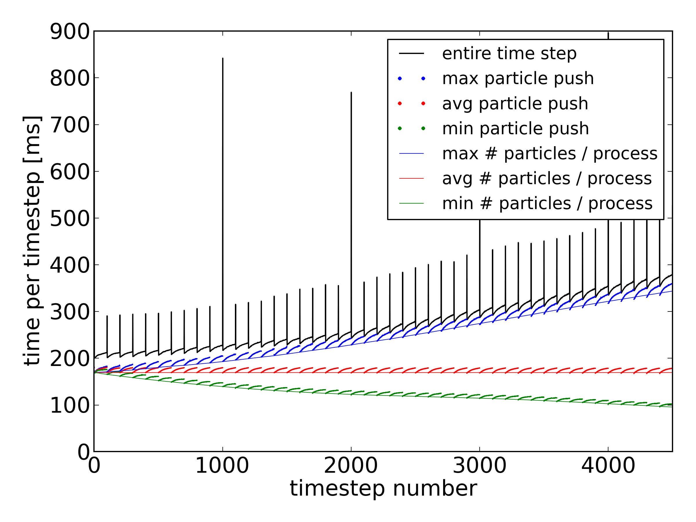
Figure 4: Computational performance over the course of a sample PIC simulation. Shown are particle push computation time at each step, min/average/max over all processes (thick green, red, blue curves), corresponding rescaled number of particles per process (thin green, red, blue curves), and total time per timestep (black).

Factors that determine the performance of a typical particle-in-cell simulation are best explained using performance data from a sample run, as shown in Fig. 4.

The performance measurements are plotted as a function of timestep. The thick jagged green, red, and blue lines are all measurements of the execution time for the particle push (including current deposition). The green curve gives the measurement from the fastest MPI process, the blue curve shows the slowest MPI process, and the red line indicates the average time over all processes. All measurements coincide in the beginning of the simulation. As the simulation runs there is an increasing spread between slowest and fastest processes, while the average performance remains approximately constant. The reason for this becomes clear when considering the number of particles on each process, which are plotted as the thin green, red, and blue lines. These data were rescaled to match the initial partitle push time. Initially, the number of particles handled by each process are equal in this simulation, but they then become unbalanced with some processes handling fewer than average, others handling more than average. The average particle number itself of course remains constant. The cause for the divergent particle push performance is clear: Particles move between MPI process boundaries, leaving some processes with more computational work in the particle pusher, and others with less.

In black we plot the total time per timestep – this number does not vary much between different processes, since processes that finish their work faster still have to wait for others to finish before communication can be completed. As expected, the total time per timestep tracks the slowest process. While unfortunate, it is the weakest link that determines overall performance, and that is why an unbalanced simulation can slow down a run substantially.

More can be learned from the data: Particle push time creeps up slightly until it suddenly falls back down to the expected level every 100 steps. That is because we sort particles by cell every 100 steps in this run – processing particles in sorted order is more cache-friendly, since $\mathbf{E}$ and $\mathbf{B}$ fields used to find the Lorentz force will be reused for many particles in the same cell before the pusher moves on to the next cell. The cost of sorting can also be seen in the total time per timestep as the small spikes in total time (black) every 100 steps. Additionally, we see larger spikes in total time every 1000 steps. These are caused by performing I/O.

4.3 Dynamic load balancing using space filling curves

In this work, we present a new patch-based approach to load balancing particle-in-cell simulations and investigate the performance costs and benefits.

The idea is easily stated: Given a number of processing elements, $N_{proc}$, decompose the domain into many more patches $N\gg N_{proc}$ than there are processing elements, and hence have each processing element handle a number of patches, typically 10 – 100. By dynamically shifting the assigment of patches to processing elements we can ensure that each processing element is assigned a nearly equal load.

We will start by demonstrating the idea in a number of idealized cases. Later, we will analyze how it performs in real-world productions.

4.3.1 Example: Uniform density

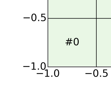
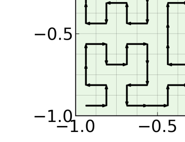
(a) (b) (c)

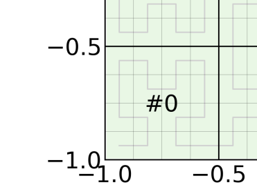
Figure 5: Basics of patch-based load balancing. The example simulation has uniform density and is parallelized to use 16 MPI processes. (a) Traditional domain decomposition into $4\times 4$ subdomains. (b) Patch-based decomposition: The domain is now decomposed into $16\times 16$ patches, and a Hilbert-Peano curve is used to assign patches to MPI processes. (c) Resulting assignment of the domain to MPI processes.

The basic idea for load balancing by using many patches per processor is demonstrated in Fig. 5. We start out with a case of uniform density. We use 16 MPI processes to run the simulation, and use standard domain decomposition to divide the domain into $4\times 4$ subdomains, one on each rank. This case is of course trivially load balanced already, since every subdomain is the same size and contains the same number of particles, see Fig. 5(a).

Still, to demonstrate our approach, we divide the domain into $16\times 16$ subdomains instead, as shown in Fig. 5(b). Since there are now many more patches (256) than processes (16), each process needs to handle multiple patches, and it is necessary to define a policy that assigns patches to processes. Fig. 5(b) also shows the Hilbert-Peano space-filling curve [39, 40]. Following along the 1-d curve, each patch is visited exactly once. The 256-patch long curve is then partitioned into as many segments as we have processes, in this case we obtain 16 segments of 16 patches each. The segments of patches are then successively assigned to each MPI process. In the end (see Fig. 5(c)), we end up with essentially the same spatial decomposition as the standard partitioning using $4\times 4$ subdomains, but we gained additional flexibility to react to changing loads by moving patches from processes with higher load to neighboring processes with lower load.

Choosing the Hilbert-Peano curve is just one option; one could, e.g., choose a simple row-major enumeration of the patches instead. As we will show later, the property that points which are close in 2-d (or 3-d) space are (on average) also close on the Hilbert-Peano curve does generally provide decompositions where the subdomain handled by a single MPI process is clustered in space, so that most communication between patches is actually local and does not require MPI communication, so that overall inter-process communication still benefits from scaling as the surface-to-volume ratio. This is the reason why space-filling curves have commonly been used to load balance block-structured adaptive mesh refinement codes [41, 42, 43], and why, as we will show, it also works well for load balancing particle-in-cell simulations.

Up to this point we have only considered a case with uniform density (which is trivially load balanced) and so our load-balancing approach does not offer any major benefit here. We have shown, that it creates a good decomposition; essentially the same that one would have chosen in a one subdomain per process approach. There are actually some potential benefits, though, that are worth mentioning: The requirement to have a specific number of processes, e.g. square numbers like $4\times 4$ can be abandoned – the same decomposition into 64 patches can be run on 64, 16, 15, or 2 processes. We envision this to be a useful feature when dealing with node failures, which are expected to become a more common problem as simulations use an increasing numbers of cores as machine performance moves towards the exascale. If one node, say 32 cores, dies in a 250,000 core run, the code would be able to continue the simulation on just 249,968 cores by redistributing patches among the remaining cores – though obviously the data on those patches need to be recovered first, which requires some kind of frequent (possibly in-memory) checkpointing.

While having many small patches on a process means increased synchronization work at patch boundaries (in particular handling ghost points and exchanging particles), most of this work is wholly within the local subdomain and so can be handled directly or via shared memory rather than by more expensive MPI communication. As we will show later, dividing the work into smaller patches can even have a positive impact on computational performance due to enhanced data locality which makes better use of processor caches.

4.3.2 Example: Enhanced density across the diagonal

(a) (b) (c)

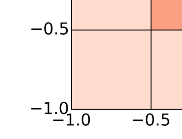
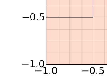
(d) (e) (f)

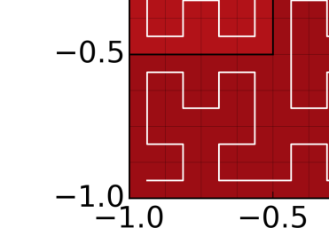
Figure 6: Load balancing increased density across the diagonal. We compare traditional domain decomposition (top row) to patch-based load balancing (bottom row). Thick black lines demarcate the subdomains assigned to each MPI process, thing grey lines show the underlying patches. (a), (d) plasma density. (b), (e) computational load for each decomposition unit. (c), (f) aggregate computational load for each MPI process.

The next example demonstrates the load balancing algorithm in action. We chose a uniform low background density of $n_{b}=0.1$ and enhance it by up to $n=1.0$ along the diagonal of the domain, as shown in Fig. 6. This density distribution is chosen to be one where the psc’s former approach to load balancing is not effective at all: After dividing the domain into $4\times 4$ subdomains it is not possible to shift the subdomain boundaries in a way that reduces load imbalance; this simulation will always be unbalanced by a factor of more than $7\times$ as shown in Fig. 6(b), (c). Subdomains near the high-density diagonal have an estimated load of 81200, while away from it the load is as low as 11300.

Patch-based load balancing, however, works quite well. The resulting decomposition is shown in Fig. 6 (d)-(f) by the thicker black lines. It can be seen that some subdomains contain only a few patches, including some with a large load (high density, i.e. many particles), while other subdomains contain more patches but mostly at a low load.

Fig. 6 (b) shows the load for each patch, which is calculated for each patch as number of particles plus number of cells in that patch – clearly this mirrors the particle density. Fig. 6 (c) plots the aggregate load per process, calculated as the sum of the individual loads for each patch in that process’s subdomain. It is clear that the load is not perfectly balanced, but it is contained within $\pm 7.5\%$ of the average load of 29300. This is certainly a vast improvement over an imbalance by a factor of more than $7\times$ in the original code.

4.3.3 Load balancing algorithm

The goal of the actual balancing algorithm is quite straightforward: Divide the 1-d space filling curve that enumerates all patches into $N_{proc}$ segments, where $N_{proc}$ is the number of processes such that all processes have approximately equal load. In order to accomodate inhomogeneous machines, we add a “capability” specification. For example, we may want to run 16 MPI processes on a Cray XK7 node. 15 of those processes run on one core each, while the last one is used to drive the GPU on the node. In this case, we would assign a capability of 1 to the first 15 processes, and a capability of 60 to the last process, since the GPU performance is roughly $60\times$ faster than a single CPU core and we want it to get correspondingly more work.

The balancing algorithm hence divides the space-filling curve into segments that approximately match the capability for each rank – in the simple case of a homogeneous machine all capabities are equal and the algorithm reduces to distributing the load equally. The algorithm is described in more detail in A.

4.3.4 Synchronization points

As previously laid out, a time step in the psc consists of a number of substeps that advance electric and magnetic fields and update particle positions and moments. Substeps depend on results from previous substeps, often not only within the local domain but (near the boundaries) also on results from remote processes. Hence communication is required and introduces synchronization points between processes, which interferes with load balancing the entire step.

While the PIC algorithm we use is naturally staggered in time for both particles and fields, the implementation in the original psc broke up all but one step into two half steps so that the timestep would start with all quantities known at time $t^{n}$, and advance them all to time $t^{n+1}$, as shown in Fig. 7.

push_field_E_half();	// $\mathbf{E}^{n}\rightarrow\mathbf{E}^{n+1/2}$
fill_ghosts_E();	// communicate
push_field_B_half();	// $\mathbf{B}^{n}\rightarrow\mathbf{B}^{n+1/2}$
fill_ghosts_B();	// communicate
foreach(particle prt) {
push_particle_x_half(prt);	// $\mathbf{x}^{n}\rightarrow\mathbf{x}^{n+1/2}$, save for current
push_particle_p(prt);	// $\mathbf{p}^{n}\rightarrow\mathbf{p}^{n+1}$
push_particle_x_half(prt);	// $\mathbf{x}^{n+1/2}\rightarrow\mathbf{x}^{n+1}$
push_particle_x_half_temp(prt);	// $\mathbf{x}^{n+1}\rightarrow\mathbf{x}^{n+3/2}$, use for current, then disregard this update
deposit_j();	// charge conservative current deposition using $\mathbf{x}^{n+1/2}$ and $\mathbf{x}^{n+3/2}$
}
exchange_particles();	// communicate
push_field_B_half();	// $\mathbf{B}^{n+1/2}\rightarrow\mathbf{B}^{n+1}$
fill_ghosts_B();	// communicate
add_and_fill_ghosts_j();	// communicate
push_field_E_half();	// $\mathbf{E}^{n+1/2}\rightarrow\mathbf{E}^{n+1}$
fill_ghosts_E();	// communicate

Figure 7: Original implementation of the timestep in psc. All quantities start at time $t^{n}$ and are advanced to time $t^{n+1}$. Communication is performed at 5 different synchronization points.

Communication occurs at 5 different points during the timestep as indicated, separated by computational kernels on either field or particles. Communication is implemented using non-blocking MPI send and receive calls; the time while messages are in flight is used to exchange field boundary data and particles between local patches that do not require inter-process communication. However, these communications still introduce synchronization points. A given process will not be able to, e.g., update the fields until current density data has been received from neighboring processes. Neighboring processes won’t be able to send these data until they finished pushing their local particles. The consequence is that it is not enough to just balance the total computational work, which includes both particle and field work. Rather, it is necessary to balance both particle work and field work individually between all processors. However, this is in general not possible.

In practice experiments showed that, for typical cases, using our approach to load balancing still worked quite well because performance is dominated by particle work, with field work being comparatively fast, so that imbalance in the field work does not cause a great loss in performance. We set up the load balancing to equally distribute the number of particles that each process handles, up to the patch granularity. In a typical case we observed a slow-down of particle-dependent kernels by about 15% over the course of the run, which is consistent with the 15% deviation in particle number balance the algorithm achieved. The overall performance, however, would slow down by 30%. Using the previous approach to load balancing by shifting process boundaries we observed a 200% slow-down in the same case, so this was still a large improvement. It does, however, show that as we balance the particle load the field load becomes imbalanced and creates a new loss of performance that manifests itself in the overall timestep slow-down.

With careful consideration, it is possible to improve balancing to include both particle and field work. The basis for the updated load balancing is to rewrite the time step closer to the natural time-staggered form in our numerical algorithms. In the new algorithm, we start a time step with the quantities known as $\mathbf{E}^{n+1/2},\mathbf{B}^{n},\mathbf{x}^{n+1/2},\mathbf{p}^{n}$, and propagate them to $\mathbf{E}^{n+3/2},\mathbf{B}^{n+1},\mathbf{x}^{n+3/2},\mathbf{p}^{n+1}$ as shown in Fig. 8.

push_field_B_half();	// $\mathbf{B}^{n}\rightarrow\mathbf{B}^{n+1/2}$
foreach(particle prt) {
push_particle_p(prt);	// $\mathbf{p}^{n}\rightarrow\mathbf{p}^{n+1}$
push_particle_x(prt);	// save $\mathbf{x}^{n+1/2}$ for current, then $\mathbf{x}^{n+1/2}\rightarrow\mathbf{x}^{n+3/2}$
deposit_j();	// charge conservative current deposition using $\mathbf{x}^{n+1/2}$ and $\mathbf{x}^{n+3/2}$
}
push_field_B_half();	// $\mathbf{B}^{n+1/2}\rightarrow\mathbf{B}^{n+1}$
exchange_particles();	// communicate
fill_ghosts_B();	// communicate
add_and_fill_ghosts_j();	// communicate
push_field_E();	// $\mathbf{E}^{n+1/2}\rightarrow\mathbf{E}^{n+3/2}$

Figure 8: Optimized implementation of the timestep in psc. It advances $\mathbf{B}^{n},\mathbf{p}^{n}\rightarrow\mathbf{B}^{n+1},\mathbf{p}^{n+1}$ and $\mathbf{E}^{n+1/2},\mathbf{x}^{n+1/2}\rightarrow\mathbf{E}^{n+3/2},\mathbf{x}^{n+3/2}$ and performs all communication at a single synchronization point.

Every quantity is now updated only once, by a full step, with the exception of $\mathbf{B}^{n}\rightarrow\mathbf{B}^{n+1/2}\rightarrow\mathbf{B}^{n+1}$, which is required at the intermediate time to interpolate the Lorentz force acting on particles.

Other than the drawback of having to handle quantities at different time levels at the initial condition and output, the scheme in its natural form presents a number of advantages: Less computational work is required due to combining half steps into full steps. The discrete version of Gauss’s Law is required to be satisfied exactly at half-integer time levels, which can now be achieved more easily in the initial condition. Particles are exchanged according to their positions at time $t^{n+1/2}$, so particles are guaranteed to actually be inside the local domain at the time that the electromagnetic fields are interpolated to the particle position. This is in contrast to the old scheme, where a particle already moved a half time step, and hence might have left the local domain. This means that fewer levels of ghost points are required.

Most importantly, the rewritten scheme can be recast to have only a single synchronization point. We now do all communication after the particle push and after completing the second half step to update $\mathbf{B}$. At that point, particles are ready to be exchanged as their positions have been advanced to $\mathbf{x}^{n+3/2}$. The current density $\mathbf{j}^{n+1}$ has been calculated and can be added up and used to fill ghost points. After we also fill ghost points for $\mathbf{B}^{n+1}$, enough information is available to perform the remaining field updates all the way to the next particle push, while still providing the necessary ghost cell data for the field interpolations in the next particle push.

For second-order particle shape functions, two layers of ghost points for the fields $\mathbf{j}$, $\mathbf{E}$, and $\mathbf{B}$ are sufficient to perform a full time step, including field and particle updates, without any further communication.

4.3.5 Calculating the load function

As the time integration now requires only a single synchronization point, it is possible to balance the total computational load per timestep, including both particle and field updates. The load balancing algorithm requires as input an estimate of the load $L_{p}$ associated with the computations occuring on each of the patches, $p$. A promising candidate is a function of the form

$$L_{p}=N_{particles}(p)+CN_{cells}(p),$$ (32)

as the work in the particle push scales with the number of particles being pushed, while the field updates scale with the number of grid cells. The constant $C$ can be used to adjust the weighting between particle push and field updates, as the work of pushing one particle is not expected to be equal to the work of advancing the fields in one cell. As we will show in a case study later, this simple approximation works quite well to achieve good balance. It requires, however, an appropriate choice of the parameter $C$, so we also pursued an alternate approach of actually measuring the time spent in the computational kernels.

4.3.6 Performance cost of subdividing the domain

Global number of patches	Patches per process	Patch size
$30\times 20$	1	$40\times 40$
$60\times 40$	4	$20\times 20$
$120\times 80$	16	$10\times 10$
$150\times 100$	25	$8\times 8$
$240\times 160$	64	$5\times 5$

Table 1: List of runs to study the performance cost of dividing the domain into many small patches.

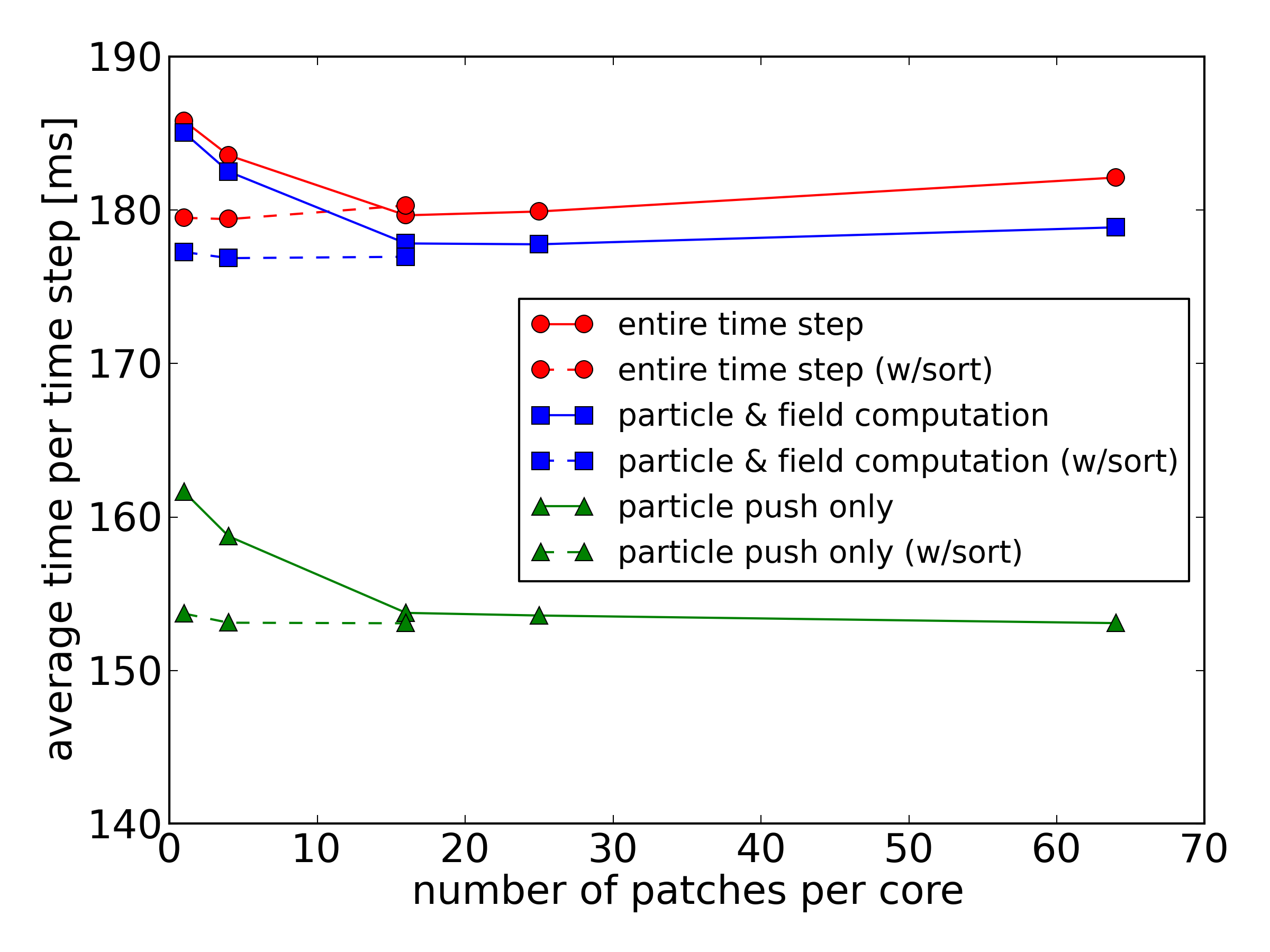
Figure 9: Timing data for naturally balanced runs while varying the number of patches that the domain is decomposed into from 1 patch per core to 64 patches per core.

Subdividing the spatial domain into many more patches than processing units can improve the load balance of a particle-in-cell simulation dramatically. On the other hand, besides the increased complexity in implementing the approach, there are also potential performance costs: (1) Rebalancing the domain, including moving patches to other processes in order to improve load balance takes processing time. (2) Handling many small patches on a process rather than just one large patch creates costs in managing those patches, in increased computational work, and in increased communication both between local patches and between local and remote patches.

While the cost of rebalancing (1) is substantial, typically equal to a couple of regular timesteps, rebalancing only needs to be performed occasionally, typically every 100 – 500 steps, so this cost gets amortized over a large number of steps. As will be shown in a case study below, we find that the cost of rebalancing only adds an amortized cost of 1–2%.

In order to address issue (2), we performed a number of simulations at identical physical and numerical parameters, while varying the number of patches that the domain is divided into. We used physical plasma parameters motivated by the bubble reconnection simulations that will be described in more detail later, but changed the initial condition to be a uniform plasma. Using a bubble simulation directly is not feasible, since the initial density is non-uniform and, even if the simulation is initially load balanced, it quickly becomes unbalanced. The initially uniform plasma remains uniform, which means that no actual load balancing is required and we can exclude the impact of growing imbalance and focus just on the peformance cost of varying the partitioning into patches. Our example case is run at a resolution of $1200\times 800$ grid cells using 600 cores, using 200 particles per cell per species. We start with a simple decomposition into $30\times 20$ patches, which means that every process handles only a single patch of size $40\times 40$ grid cells. In this case there is no additional cost from subdividing the domain into smaller patches, it is just standard domain decomposition. We then increase the number of patches the domain is divided into progressively up to $240\times 160$, i.e. 64 patches per process of size $5\times 5$ each. Table 1 lists the parameters for the simulations we performed.

Fig. 9 plots average performance data vs the number of patches per MPI process. The first thing to notice is that the variation of the total time per time step (red curve with circles) is fairly small: it varies between 179.4 ms and 185.8 ms, i.e., the slowest case is less than 4% slower than the fastest. The plotted data were obtained by averaging the timing measurements over simulation time steps 500 to 1000 (we skipped the initial 500 steps in order to avoid measuring transients from the initial condition.) At each time step, psc measures the wallclock time to perform certain work, and then finds minimum, maximum and average over all MPI processes. We show the maximum values in the plot, as the slowest processes generally determine overall performance, though there is little variation between minimum, maximum and average as the simulation is naturally balanced.

The total time per time step initially goes down (solid red curve) as the number of patches is increased up to 16 patches per process, and then goes up again. This might seem surprising, but is easily explained by the limited cache memory available to each core. As the patch size decreases to $10\times 10$, field data is more effectively cached – all particles in any one patch are processed before moving on to the next patch, so the fields will quickly become resident in cache, allowing to push all particles in that patch without further access to field data in main memory. We confirm this by looking at the total computational work per timestep (blue curve with squares) and the particle push time (green curve with triangles). It is clear that the faster total time per time step originates in the particle pusher. The clearest evidence comes from re-running the simulations with particle sorting enabled every 50 steps (dashed lines). Since particles are now always sorted, fields are accessed in a structured manner independent of the patch size, and we consistently see fast performance. With sorting enabled, performance is now in fact fastest when using only one patch per processor, avoiding the additional overhead of multiple patches. However, the performance cost of using many patches is very small. Even at 64 patches / core, which corresponds to a very small patch size of $5\times 5$ grid cells, the time step is only 1.5% slower than in the fastest case. This performance loss, small as it is, can be traced down to two causes: (1) The total computational work per timestep (blue curve) increases – this is mainly caused by the additional ghost cells that Maxwell’s equations are solved in (as we laid out before, some ghost cell values are calculated rather than communicated to avoid additional communication and synchronization points). (2) The time spent exchanging particles and ghost cell values increases. This time can be seen in the figure as the difference between the blue and the red curve, and it clearly increases as the number of patches per core increases. Most of the additional communication occurs between patches on the same MPI process, where it is handled by simple copies, rather than actual message passing, which keeps its overall impact small.

From the data we presented here, it is clear that the overhead of using many patches per process remains quite small as long as the patch size is not made unreasonably small.

4.4 Performance study: Load balancing a bubble reconnection simulation

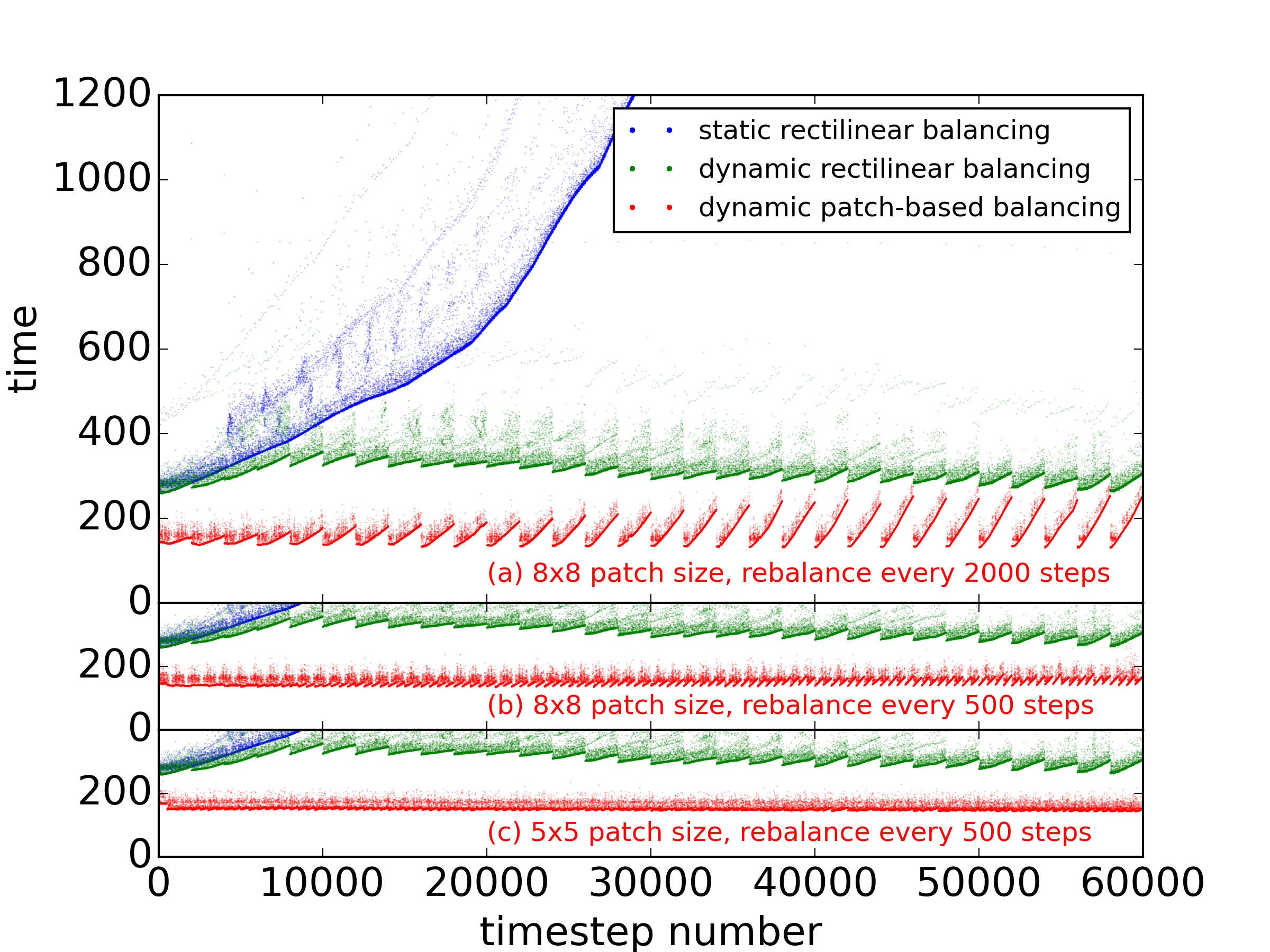
Figure 10: Wall clock time per timestep for runs with static rectilinear (blue), dynamic rectilinear (green), and dynamic patch-based (red) load balancing.

Our first case for studying the utility and performance of the space-filling curve based load balancing scheme in psc is a simulation of magnetic reconnection of laser-produced plasma bubbles. More detail about those simulations and the underlying physics can be found in [9, 10]. The runs presented below used a background plasma density of 0.1 and a peak density of 1.1 in the center of the bubbles in normalized units. The plasma bubbles expand into each other, driving magnetic reconnection; in the process, the peak density moves from the bubble center to the edge. We used a mass ratio of $m_{i}/m_{e}=100$. The domain size is $60d_{i}\times 40d_{i}$, we use $2400\times 1600$ grid cells. All runs were performed using 2048 cores of the Cray XE6m supercomputer Trillian located at the University of New Hampshire. We will compare 4 approaches to domain decomposition and load balancing: (1) uniform decomposition, (2) static rectilinear decomposition, (3) dynamic rectilinear decomposition, and (4) dynamic patch-based decomposition.

4.4.1 Uniform decomposition

This easiest approach, i.e. dividing the domain into as many equal-sized subdomains as there are processors (see Fig. 3), does not afford any opportunity to balance the computational load, which ends up being substantially unbalanced at a factor of $11\times$. This actually made it infeasible to run a complete simulation, and the timing was so far off compared to the other methods that we chose to scale Fig. 10 to focus on the results from the more promising load balancing methods.

4.4.2 Rectilinear balancing

Figure 11: Rectilinar decomposition by shifting decomposition boundaries. (top) at the initial time, (bottom) shifted decomposition after time of maximum reconnection rate at 50,000 steps. Show in green is the plasma density

As mentioned earlier, PSC originally supported what we call “static rectilinear load balancing”. That is, at initial set up time the decomposition boundaries are shifted along the coordinate axes to achieve better load distribution as shown in Fig. 11 (top). This decomposition substantially improves load balance – initial imbalance is now down to less than $2\times$. Fig. 10 compares rectilinear load balancing to our new patch-based approach, showing the evolution of the compute time per timestep. The statically balanced case (blue) starts out $1.7\times$ slower than the patch-based approach, but load balance quickly increases. As originally implemented, there was no dynamic rebalancing, so the slow-down was drastic once the bubble dynamics substantially changed the plasma configuration, and we did not continue the solution past the halfway point.

We added the capability to dynamically rebalance the rectilinear approach, which is shown by the green curve. The effect of rebalancing every 2000 steps can be clearly seen – imbalance still grows initially, but is then arrested and is remains under $2.5\times$. While not ideal, this allowed us to perform these kind of simulations to completion.

4.4.3 Patch-based balancing

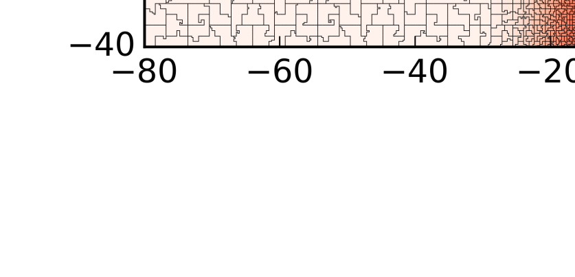
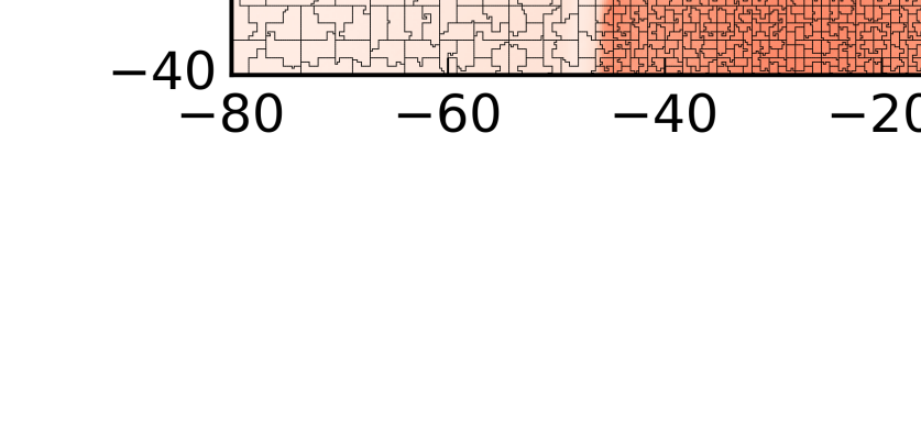
Figure 12: Patch-based load balancing. (top) at the initial time, (bottom) shifted decomposition after time of maximum reconnection rate at 50,000 steps. Show in red is the actual load per patch, which follows the number of particles and plasma density, and the decomposition boundaries (black).

The resulting decompositions from using the patch-based approach are shown in Fig. 12. The figures shows that the per-MPI process subdomains (demarcated by black lines) are indeed well clustered in space by means of using the space-filling curve. Local subdomains range from encompassing many ($\sim 100$) low-density patches down to just 4 of the highest density patches. As shown in red on Fig. 10, we achieve rather good load balance using this new method and are able to maintain it in time given the right parameters.

Fig. 10 compares three different runs. (a) used patches of size $8\times 8$ grid cells, rebalancing every 2000 steps. It can be seen that at later times the load quickly becomes unbalanced again after each rebalancing step, so better average balance is obtained using more frequent rebalancing as shown in (b) at every 500 steps. Finally, in (c) we used more, even smaller patches of size of $5\times 5$ which, in fact, still worked very well. As expected the load balance improves a bit, while the increased overhead does not substantially affect performance.

4.4.4 Timing comparison

balancing method initial first 30,000 steps all 60,000 steps uniform $9.9\times$ n/a n/a static rectilinear $1.66\times$ $3.64\times$ n/a dynamic rectilinear $1.66\times$ $1.94\times$ $1.87\times$ dynamic patch-based $1\times$ $1\times$ $1\times$

Table 2: Slow-down of various load balancing methods compared to dynamic patch-based method.

The clearest indication of how well our new load balancing method works is given by comparing overall timing of the runs. In Table 2, we list overall timing information, comparing uniform, static and dynamic rectilinear, and patch-based balancing. Data are normalized by the performance of the new patch-based approach, i.e. we show the slow-down compared to this method. As previously mentioned, the uniform (not balanced) approach is very expensive for our test case, so we did not run a simulation beyond an initial phase where it was almost $10\times$ slower than the patch-based method. The rectilinear approaches do quite well initially, with only a slowdown of $1.7\times$. Static balancing, however, is not sufficient: The simulation down to 30,000 steps was $3.6\times$ slower and rapidly degraded even more, so that we did not continue it all the way to the end. The dynamic rectilinear approach performed reasonably well, with the simulation running not quite two times longer than the new approach.

Overall, we showed that our new patch-based load balancing approach works very well and is in fact clearly superior over the alternate methods that previously existed in psc.

4.4.5 Estimating the load

We used this test case to also compare different methods of estimating the computational load per patch, which is needed as input to the load balancing mechanism. We tried formula Eq. (32) with $C=1$ and $C=2$ and also compared it to a real time load estimator that instead of using an analytic formula actually measured timing data as the simulation proceeded. We did not observe any significant differences in the achieved balance, though we noticed that the timing data was somewhat noisy so the achieved load balance in that case would bounce around to some small extent.

4.5 Performance study: Load balancing a particle acceleration study

(a)

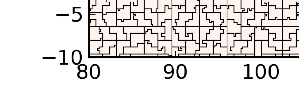
(b)

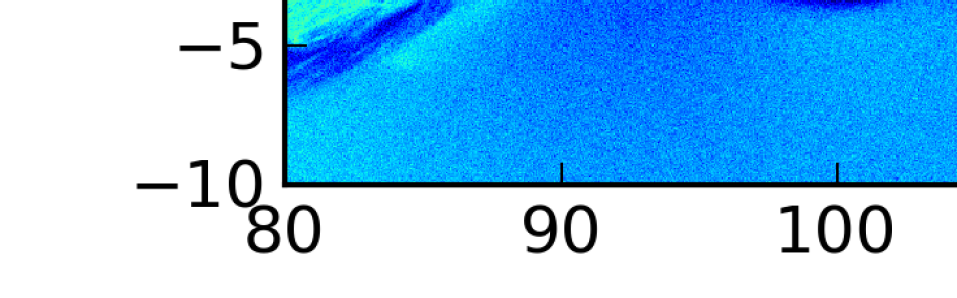
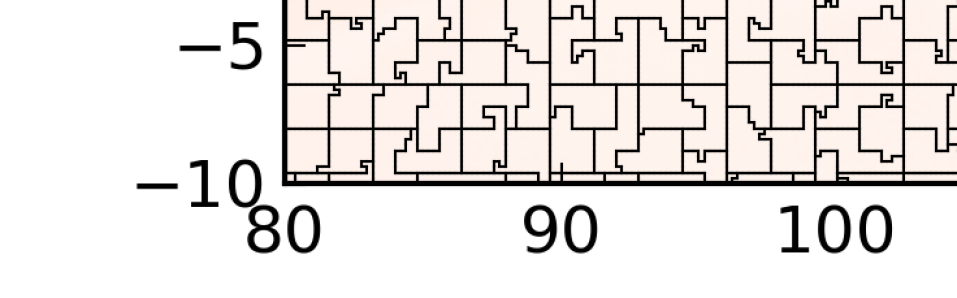
Figure 13: (a) Initial Harris sheet and (b) reconnection in progress after 70000 steps. Shown are the density on a logarithmic scale (top), and the load for each patch and the subdomain boundaries (bottom). Show is a zoom into the central region of the current sheet.

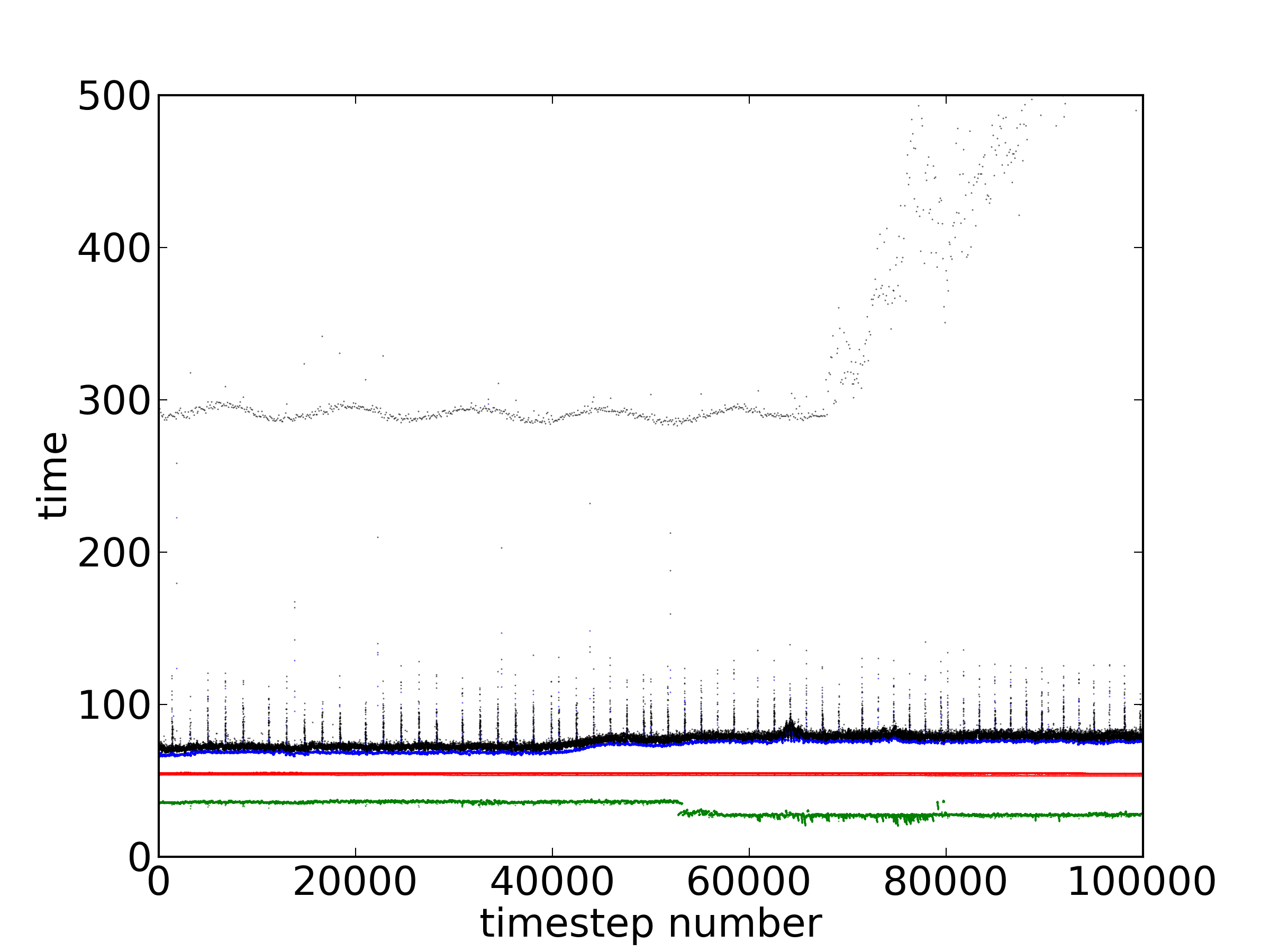
Figure 14: Timing data for the particle acceleration run, with dynamic load balancing performed every 100 timesteps. The execution time for the entire timestep is plotted in black. The time spent in actual computation is shown in blue, red and green for the slowest, average and fastest process, respectively

We performed another performance study on a simulation of particle acceleration in magnetic reconnection, to show that load imbalance can be significant in a more common application, too. The simulation parameters used here are motivated by the work in [2]. The initial condition is a Harris sheet with a central density of $n=1$ and a background density of $n=0.05$. The domain size is $204.8d_{i}\times 51.2d_{i}=4096d_{e}\times 1024d_{e}$ using a $16384\times 4096$ cell mesh. The mass ratio is $m_{i}/m_{e}=400$. We used 200 particles per cell to represent $n=1$ and the 2nd order particle shape function.

This simulation poses substantial challenges for maintaining load balance. Initially the plasma density away from the current sheet is $20\times$ lower than in the central current sheet, shown in Fig. 13(a). Consequently the load per patch is similarly unbalanced, varying from 1344 to 26592 in the center, a ratio of $19.8$. The simulation divides the domain into $1024\times 256=262144$ patches of $8\times 8$ cells, and is run on 8192 cores. This averages to 32 patches / core, but due to the strong imbalance the achieved load balance is only within $\pm 32\%$ – still a vast improvement over the original $20\times$.

As the simulation proceeds load balancing becomes even more challenging since reconnection occurs, some plasmoids form and get ejected, and almost all of the density gets concentrated in few islands while the plasma in the rest of the domain becomes very tenuous.

After 70000 steps (see Fig. 13(b)), the load varies from a minimum of 228 to a maximum of 52011, an imbalance of $230\times$. The code handles the increasing load balance quite well, though, balancing process load to within $\pm 50\%$.

Fig. 14 shows the timing information throughout the run. The black curve again indicates the execution time of an entire timestep – it only increases mildly at around 50000 steps, which is when plasmoids start forming, and then remains approximately flat again thereafter. We again see that the black line is only slightly above the blue line, the computational time used on the process with the heaviest load. This indicates that communication / boundary exchange is not a significant performance factor. The spread of the green (fastest) and blue (slowest) process from the average (red) indicates that load balance is not perfect, in fact these mirror the aforementioned $\pm 32\%$, $\pm 50\%$ deviation from perfect balance. This spread is certainly acceptable considering that the underlying imbalance is greater than $200\times$. The faint black dots at around 300 ms are slower time steps that include rebalancing – these occur every 500 steps and have a noticable cost, but don’t affect the overall performance significantly.

5 GPU algorithms

5.1 Introduction

Originally designed to speed up processing and display of images on computer screens, graphics processing units (GPUs) have, in recent years, evolved into powerful processors that can accelerate general computationally-intensive tasks. Optimized for highly parallel computations, they have shown potential to accelerate numerical simulation codes significantly. The two fastest supercomputers in the world, according to the TOP500 list from June 2015 [44], and many others down the list derive their computing capabilities from accelerator technology like Nvidia GPUs and Intel’s Many-Integrated-Cores (Xeon Phi) processors. DOE’s supercomputer Titan consists of 18,688 nodes with one 16-core AMD 6274 CPU and one Nvidia Tesla K20X GPU each. About 90 % of its theoretical capability in floating point operations per second are provided by the GPUs, which clearly shows that only GPU-enabled codes can get close to using all of its potential.

GPUs and other accelerator technologies hold great promise in enhancing scientific discovery through their increased computational power, but they come with challenges to adopt codes to efficiently use their theoretical capabilities. Different programming models exist, from using provided libraries (e.g., cudaBLAS) through relatively minor changes to existing code using an annotation-based programming model like OpenACC to rewriting computational kernels from scratch using CUDA C/C++ or CUDA Fortran.

Most of the existing work [45, 46, 47, 48, 49] on porting particle-in-cell codes to GPUs focuses on basic algorithms, e.g., electrostatic simulations where only the charge density needs to be deposited back onto the grid and work is performed more in proof-of-concept codes rather than full-scale production codes. psc uses charge-conservative current deposition, as also discussed in [48]. We added GPU capabilities to the psc code based on its existing modular architecture that enabled us to implement new computational kernels as well as new underlying GPU data structures within the existing code. In the particle-in-cell method, the important computational work generally scales linearly with the number of particles and is of low to moderate computational intensity, which means that copies between main memory and GPU generally have to be avoided to achieve good performance. Therefore, the simpler programming approach of keeping most of the code and data structures on the host CPU unchanged and using the GPU to just accelerate selected kernels is not feasible.

psc has been run using first order single precision particles in a 2-d simulation on thousands of GPUs and achieved a performance of up to 830 million particles / second per node on Titan using the Nvidia K20X GPUs, which is more than six times faster than its performance on the CPUs only.

While psc’s 2-d GPU capabilities are mature and have been used in production runs, 3-d support and support for higher order particle shapes on GPUs is still under development. We therefore only briefly introduce the various GPU-ported algorithms in the following, and will provide a comprehensive performance evaluation for 2-d and 3-d in a future publication.

As on CPUs, the kernels that dominate the overall performance are particle related kernels, in particular: particle advance and field interpolation, current deposition as well as sorting.

5.2 Particle Advance and Field Interpolation

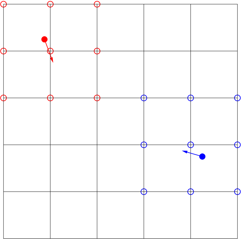
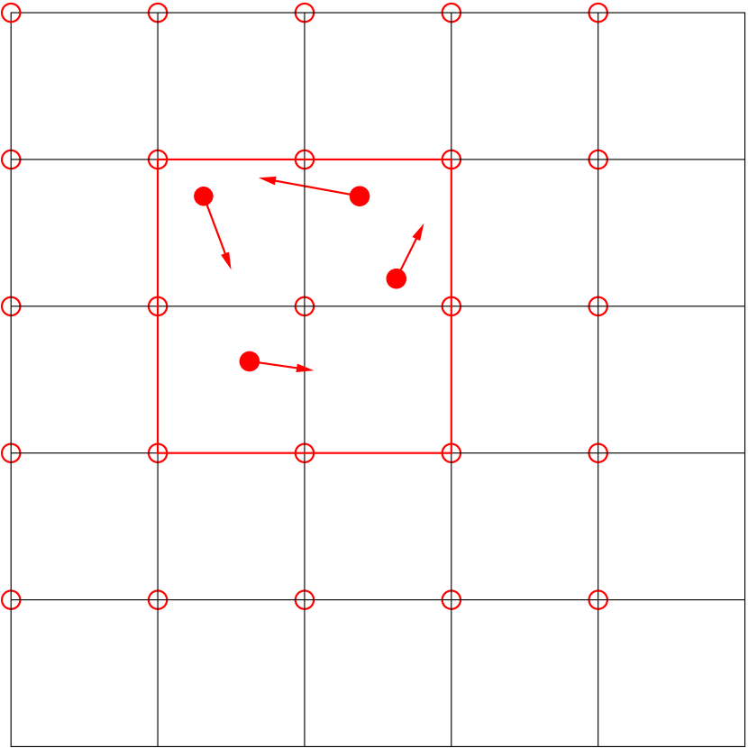
Figure 15: Processing particles on the GPU. (a) If particles are unsorted (left): to interpolate electromagnetic forces to the particle position, field values need to be loaded from global memory for the grid points surrounding each particle. (b) If particles are sorted (right) by super-cell (red square), all required field values can be loaded into shared memory (red circles) first and then be used to interpolate forces for all particles.

The particle advance consists of two components: Stepping the equations of motion in time, and calculating the currents from the particle motion, which act as a source term to Maxwell’s equations.

The equations of motion can be solved for each particle independently of all the other particles, making the particle push itself highly parallel. The particles do not interact directly, but only through the electromagnetic fields. Each particle push requires finding electromagnetic field values on grid locations in the vicinity and interpolating them to the particle location. While many particles may access the field values in the same grid location concurrently, these are read-only accesses that do not require serialization.

For performance reasons it is advisable to avoid accessing the field values in random order, which leads to a memory access bottleneck. On traditional CPUs, many cache misses will occur and performance can degrade greatly. Figure 15(a) depicts this effect. For each particle, field values from surrounding grid points need to be loaded to find the Lorentz force. As particles are accessed in random order, these accesses are all over the place. Similarly, current density updates go back to main/global memory in random order. Avoiding random memory accesses is the reason that particles are kept approximately sorted by grid cell in most PIC codes. As sorted particles are accessed sequentially on a single process (or thread), most of the field values will already be in cache.

On GPUs, it is most efficient to keep particles strictly sorted and use shared memory for field access. It is generally sufficient to sort particles by super-cell (e.g., a block of $2\times 2$ cells in 2-d). Fig. 15(b) shows all particles in a given $2\times 2$ super-cell – in this example, we show just 4 particles for simplicity, though we usually have many more particles in a super-cell. A CUDA threadblock will load all field values needed into shared memory first, then push all particles in that super-cell, before continuing on to the next super-cell and repeating the process. A super-cell in a production run typically contains thousands of particles, so the cost of loading the fields from global memory is amortized over all those particles.

Benchmarks comparing super-cells of sizes $1\times 1$, $2\times 2$, $4\times 4$, $8\times 8$, and $16\times 16$ showed a performance gain of up to $2.5\times$ to $5\times$ compared to no shared memory caching, where the best performance was achieved with $4\times 4$-sized supercells. Supercells of very small sizes are suboptimal for two reasons: Field loads are not amortized over a sufficiently large number of particles in the supercell, and the smaller number of particles also does not provide enough fine-grained parallelism for the GPU to exploit. On the other hand, using very large super-cells, we encounter limitations in the amount of available shared memory, which limits the number of concurrent threadblocks.

On Nvidia K20X hardware, using a 1st order particle shape, we achieve an impressive performance of 2290 million particles per second for the particle push itself, which includes interpolation of the electromagnetic fields and updating positions and momenta (but not the current deposition).

5.3 Current deposition

Implementing a highly-parallel GPU current deposition algorithm is substantially more difficult than the particle push. Each particle, as it moves, contributes to the current density, which is accumulated on the field mesh. In doing so, we have to find the corresponding current for each particle and deposit it onto nearby grid locations according to the particle’s shape function. The deposit is a read-modify(add)-write operation. As multiple particles are processed in parallel, they may modify the same grid value concurrently depending on their exact position in the domain. It is therefore necessary to introduce synchronization to ensure that multiple threads do not update the same value at the same time and lose contributions. Our experience mirrors that of [48, 49]; we found that the most efficient way to handle this problem is to use atomic_add() in shared memory on Nvidia Fermi and newer compute architectures.

It is still important to avoid getting many memory conflicts. Even though atomic_add() guarantees correctness, performance slows down when frequent memory access collisions occur. Sorting only by a not-too-small super-cell rather than ordering by cell helps. The GPU will process 32 particles in one warp – if all of those particles are in the same cell, chances that multiple threads want to update the same current density value are much higher than if those 32 particles are randomly spread inside, e.g., a $4\times 4$ super-cell. We actually observed the current deposition speed up by a factor of 2 during the initial phase of the simulation as particles, which are initially ordered by cell when setting up initial conditions, randomize by their thermal motion and mix within the super-cells. Conflicts, of course, could be avoided entirely if every thread was to write into a private copy of the current density field, in this case it is not even necessary to use the atomic updates – though in the end it is necessary to add up values from all private copies, but that is generally quite fast. There is, unfortunately, not enough shared memory available in current GPU hardware to be able to support that many private copies, even in 2-d, without severely reducing the occupancy of the GPU multiprocessors and thus greatly reducing performance. It is, however, possible to maintain a limited number of redundant copies in shared memory, which reduces conflicts in the atomic operations while maintaing good occupancy. In 2-d we typically use 16 redundant copies, which increased performance almost two-fold.

We also tried alternative approaches using reductions in shared memory rather than the atomic add, but obtained our best performance for an atomic Villasenor-Buneman charge-conservative current deposition [20]. On the Nvidia K20X, we achieve a performance of 1970 million particles per second for the current deposition. Our implementation of the current deposition avoids thread divergence, i.e., different threads do not execute different if branches, though some threads may, via predicates, skip instructions.

The combined performance of particle push and current deposition is up to 1060 million particles per second. These two algorithms comprise all the particle computational work, and the Maxwell solver is typically only an insignificant fraction of the overall computational effort. However, as mentioned before, these algorithms require particles to be sorted by super-cell and, in a parallel run involving multiple GPUs, it is also necessary to exchange particle and field values across computational domains, which means an overall performance of greater than 1 billion particles per second per GPU could not actually be attained.

5.4 Sorting and Communication

On cache-based architectures, sorting particles is used to maintain cache-friendly access patterns; however, having particles slightly out of order will only incur a small performance penalty, so the cost of sorting is often amortized over tens of timesteps.

On the GPU, we essentially use shared memory as a user-managed cache, e.g., loading electromagnetic field data for a super-cell worth of particles into shared memory first, then processing all those particles directly using the field data in the shared memory. It is thus necessary to have particles sorted by super-cell before performing the particle push, because having particles out of order does not just incur a performance penalty but will rather lead to incorrect results or crashes.

Therefore, particles need to be sorted at each timestep. Like on the CPU, we also need to handle particle exchange across patch boundaries: particles that leave the local patch need to be moved to their new home patch, which may be on the same GPU, but also might be a patch on another node requiring MPI communication. In order to reduce the number of memory accesses, we handle sorting and boundary exchange in one fused algorithm.

The basis for this algorithm is a high performance GPU sort, which in itself is a complex problem due to the need to exploit a lot of parallelism to achieve good performance on GPUs.

Fortunately, efficient algorithms are available for sorting particles by cell: Sorting $N$ particles into $M$ cells a counting sort takes $\mathcal{O}(N+M)$ steps, which in the typical case of many particles per cell becomes $\mathcal{O}(N)$. The usual limit of $\mathcal{O}(N\log N)$ does not apply since the sort is not comparison-based. Here and in the following we talk about sorting by cell, which depending on the degree of sorting we need is also used to refer to sorting by super-cell. It is possible to achieve an ordering by cell and super-cell simultaneously by appropriate choice of the cell index used as sort key.

A counting sort is not directly usable on the GPU. Instead, we base our implementation on a radix sort algorithm, which splits the sort into multiple phases: In decimal notation, one could sort a list of numbers first by least significant digit (1s) only. The partially sorted numbers are then sorted by the next digit (10s), and so on, until all digits have been processed. The thrust library implements this radix sort [50], sorting 4 bit “digits” at a time using essentially a parallel counting sort for each digit. For typical simulation sizes, we would have to use 4 passes to sort the up to 16-bit keys.

We achieved a large improvement over the original radix sort by exploiting a particular property of the explicit relativistic particle-in-cell method: In a single timestep, a particle can move at most into a neighboring cell, as its speed is limited to the speed of light and the timestep is limited by the corresponding CFL condition. Hence, particles which are initially sorted by cell will still be “almost ordered” after the timestep. In fact, for each particle in 2-d there are only 9 possibilities: The particle remains in the same cell, or moves into any of the adjacent cells, including diagonals. We add one other option: The particle leaves the current patch entirely and needs to be moved to a neighboring patch. Those 10 possibilities can be represented by just 4 bits, allowing us to perform to modify the sort algorithm to just take a single radix sort pass. In 3-d, there are 27 + 1 possibilities, which again can be handled by a single efficient 5 bit pass. In 2-d, using only a single pass rather than 4 passes increases performance by almost $4\times$.

5.4.1 Fusing of GPU kernels

Going through the list of all particles is expensive due to the limited memory bandwidth – a 1st order PIC method is marginally memory-bound to start with, so having to repeat the particle memory accesses quickly creates a significant performance penalty.

While not desirable from an implementation perspective due to the ensuing complexity, numerically separate steps are best fused together. In particular, there is only one loop each time step that reads and writes all particle data: The main particle advance loop combines field interpolation, particle advance, current deposition, reordering into a sorted list, as well as calculating the sort key for a given particle to be used in the subsequent sort. The sort step itself only acts on keys and indices, calculating for each particle its new position in the list, but postponing the actual reordering to the next particle advance kernel.

Similarly, the sort and particle exchange are deeply intertwined to achieve optimal performance. Part of the first phase of the sort is to count how many particles will end up in each super-cell – at this point, it is also determined how many particles are leaving the patch and need to be exchanged. These particles are aggregated and exchanged, while the GPU runs the second phase of the sort, i.e., determining target positions for each particle. Once the newly arriving particles arrive, space is reserved for them in their respective super-cell, and finally the sort is completed.

While we have now described the fundamental ideas used in the GPU implementation, the details of the actual implementation of these fused algorithms are beyond the scope of this paper and will be published separately.

5.5 GPU Performance and Scalability

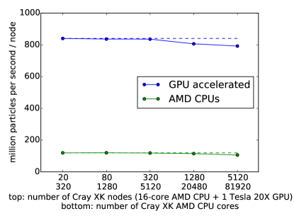
Figure 16: Weak scaling study of psc on Titan, using from 20 to 5120 16-core nodes with one GPU each, and correspondingly to 320 to 81920 CPU cores for CPU-only runs.

Fig. 16 characterizes psc’s overall scalability, comparing CPU-only to GPU-enabled runs. This weak scaling study shows that parallel efficiency is maintained at better than $90\%$ scaling up from 20 GPUs to 5120 GPUs, or correspondingly scaling from 320 CPU cores to 81920 CPU cores. The dramatic speed-up of over $6\times$ gained by using the GPUs is also clearly visible.

6 Conclusions

In this paper, we have described the numerical and computational methods used in the explicit electromagnetic particle-in-cell code psc. We have shown that it can make use of the capabilities of today’s massively parallel super-computers and can be run on 10,000’s or 100,000’s of conventional cores. psc’s flexible design allows for changing algorithms and data structures to support current and future processor designs. We have focused on two distinguishing features of psc: First, support for patch-based dynamic load-balancing using space-filling curves, which effectively addresses performance issues in simulations where large numbers of particles move to different regions of the spatial domain, causing imbalance of the computational load on the decomposed domain. Using two case studies, we have shown that psc’s new load balancing method achieves and maintains good computational performance over the entire run.

Second, psc supports Nvidia GPU’s, achieving a speed-up of more than $6\times$ on Cray XK7 nodes for 2-d problems. We have introduced the basic computational techniques applied to achieve high performance for particle-in-cell simulations not only on a single GPU, but on supercomputers with 1000s of GPUs.

psc encompasses both production and development capabilities in one code, allowing for state-of-the-art science simulations while at the same time, experimental new features are being developed. For example, while we are working on stabilizing 3-d GPU support and getting it production-ready, another effort is underway to implement support for Intel’s new many-integrated-cores processor technology (Intel Xeon Phi) which takes advantage of their 512-bit SIMD capabilities. It remains unclear where exactly the path of high-performance computation on the way to exa-scale leads, but it is fairly clear that it will involve specialized number-crunching hardware, rather than just conventional cores. So far, the approach that we have taken with psc is to use hardware-specific programming models, e.g., CUDA on GPUs or SIMD intrinsics on Intel MIC. Since only the most performance-intensive kernels need to be ported, this approach is manageable but still work-intensive. In the future, we hope to be able to leverage abstracted programming models like OpenACC/OpenMP, which fit well into the existing modular design of the code.

7 Acknowledgements

This research was supported by DOE grants DE-SC0006670 and DE-FG02-07ER46372, NSF grants AGS-105689 and and NASA grant NNX13AK31G.

Computational work has been performed on DOE’s Titan machine at ORNL and NERSC systems, and the Cray XE6m Trillian at the University of New Hampshire, funded with support from NSF’s MRI program under PHY-1229408. An award of computer time was provided by the Innovative and Novel Computational Impact on Theory and Experiment (INCITE) program. This research used resources of the Oak Ridge Leadership Computing Facility, which is a DOE Office of Science User Facility supported under Contract DE-AC05-00OR22725.

The authors acknowledge helpful discussions with Homa Karimabadi, Bill Daughton and Vadim Roytershteyn.

Appendix A Load balancing algorithm

The load balancing algorithm takes as input an array of the loads for each patch $L$, and a list of capabilities for each process rank $C_{r}$. The output is an array of the patch count $N_{r}$ that each process rank is assigned.

L_total = sum(L)	// $L_{total}=\sum_{p}L_{p}$
C_total = sum(C)	// $C_{total}=\sum_{r}C_{r}$
T_hat = L_total / C_total	// target load per unit capability
r = 0	// start by finding work for rank 0
N_cur = 0	// number of patches assigned to current rank $r$
L_cur = 0	// load assigned to current rank $r$
for p in range(N_patches):	// loop over all patches $p=0,\ldots,N_{patches}-1$
L_cur += L[p]	// tentatively assign current patch $p$ to rank $r$
N_cur += 1
if r < N_procs - 1:	// if $r$ is not yet the last process rank
	// check whether we should move on to the next rank
T_cur = T_hat * C_r	// target load for current rank $T_{cur}=\hat{T}\cdot C_{r}$
if (L_cur > T_cur or	// load target is exceeded or
N_procs - r >= N_patches - p):	// we have only as many patches as procs left
above_target = L_cur - T_cur	// including current patch, we exceed the target by this
below_target = T_cur - (L_cur - L[p])	// excluding current patch, we miss the target by this
if (above_target > below_target and
nr_new_patches > 1):	// if we were closer to the load target without the current patch,
	// assign patches up to the current one to the current process rank
N[r] = N_cur - 1
N_cur= 1
else:	// else, assign patches including current one to the current rank
N[r] = N_cur
N_cur = 0
r += 1	// move on to next rank
if p == N_patches - 1:	// last proc takes what’s left
N[N_proc - 1] = N_cur

References

- Egedal et al. [2013] J. Egedal, A. Le, W. Daughton, A review of pressure anisotropy caused by electron trapping in collisionless plasma, and its implications for magnetic reconnection, Physics of Plasmas (1994-present) 20 (2013) –.
- Egedal et al. [2012] J. Egedal, W. Daughton, A. Le, Large-scale electron acceleration by parallel electric fields during magnetic reconnection, Nature Physics (2012).
- Chacón et al. [2013] L. Chacón, G. Chen, D. Barnes, A charge- and energy-conserving implicit, electrostatic particle-in-cell algorithm on mapped computational meshes, Journal of Computational Physics 233 (2013) 1 – 9.
- Lapenta [2012] G. Lapenta, Particle simulations of space weather, Journal of Computational Physics 231 (2012) 795 – 821.
- Bowers et al. [2008] K. J. Bowers, B. J. Albright, L. Yin, B. Bergen, T. J. T. Kwan, Ultrahigh performance three-dimensional electromagnetic relativistic kinetic plasma simulation, Physics of Plasmas 15 (2008) 055703.
- Fonseca et al. [2002] R. A. Fonseca, L. O. Silva, F. Tsung, V. K. Decyk, W. Lu, C. Ren, W. B. Mori, S. Deng, S. Lee, T. Katsouleas, et al., Osiris: A three-dimensional, fully relativistic particle in cell code for modeling plasma based accelerators, in: Computational Science—ICCS 2002, Springer, 2002, pp. 342–351.
- Nieter and Cary [2004] C. Nieter, J. R. Cary, Vorpal: a versatile plasma simulation code, Journal of Computational Physics 196 (2004) 448 – 473.
- Ruhl [2006] H. Ruhl, Classical particle simulations, in: M. Bonitz, D. Semkat (Eds.), Introduction to Computational Methods in Many Body Physics, Rinton Press, 2006.
- Fox et al. [2011] W. Fox, A. Bhattacharjee, K. Germaschewski, Fast magnetic reconnection in laser-produced plasma bubbles, Phys. Rev. Lett. 106 (2011) 215003.
- Fox et al. [2012] W. Fox, A. Bhattacharjee, K. Germaschewski, Magnetic reconnection in high-energy-density laser-produced plasmas, Physics of Plasmas 19 (2012) 056309.
- Fox et al. [2013] W. Fox, G. Fiksel, A. Bhattacharjee, P.-Y. Chang, K. Germaschewski, S. X. Hu, P. M. Nilson, Filamentation instability of counterstreaming laser-driven plasmas, Phys. Rev. Lett. 111 (2013) 225002.
- Fiksel et al. [2014] G. Fiksel, W. Fox, A. Bhattacharjee, D. H. Barnak, P.-Y. Chang, K. Germaschewski, S. X. Hu, P. M. Nilson, Magnetic reconnection between colliding magnetized laser-produced plasma plumes, Phys. Rev. Lett. 113 (2014) 105003.
- Bessho et al. [2015] N. Bessho, L.-J. Chen, K. Germaschewski, A. Bhattacharjee, Electron acceleration by parallel and perpendicular electric fields during magnetic reconnection without guide field, Journal of Geophysical Research: Space Physics (2015) n/a–n/a. 2015JA021548.
- Wang et al. [2015] L. Wang, A. H. Hakim, A. Bhattacharjee, K. Germaschewski, Comparison of multi-fluid moment models with particle-in-cell simulations of collisionless magnetic reconnection, Physics of Plasmas 22 (2015) –.
- Birdsall and Langdon [1991] C. Birdsall, A. Langdon, Plasma Physics Via Computer Simulation, Series in plasma physics, Taylor & Francis, 1991.
- Hockney and Eastwood [1981] R. Hockney, J. Eastwood, Computer Simulation Using Particles, McGraw-Hill, 1981.
- Greengard and Rokhlin [1997] L. Greengard, V. Rokhlin, A fast algorithm for particle simulations, Journal of Computational Physics 135 (1997) 280 – 292.
- Yee [1966] K. Yee, Numerical solution of initial boundary value problems involving maxwell’s equations in isotropic media, Antennas and Propagation, IEEE Transactions on 14 (1966) 302–307.
- Boris [1970] J. Boris, Acceleration calculation from a scalar potential, 1970.
- Villasenor and Buneman [1992] J. Villasenor, O. Buneman, Rigorous charge conservation for local electromagnetic field solvers, Computer Physics Communications 69 (1992) 306–316.
- Esirkepov [2001] T. Esirkepov, Exact charge conservation scheme for particle-in-cell simulation with an arbitrary form-factor, Computer Physics Communications 135 (2001) 144 – 153.
- Sokolov [2013] I. V. Sokolov, Alternating-order interpolation in a charge-conserving scheme for particle-in-cell simulations, Computer Physics Communications 184 (2013) 320 – 328.
- Evstatiev and Shadwick [2013] E. Evstatiev, B. Shadwick, Variational formulation of particle algorithms for kinetic plasma simulations, Journal of Computational Physics 245 (2013) 376 – 398.
- Langdon [1992] A. B. Langdon, On enforcing Gauss’ law in electromagnetic particle-in-cell codes, Computer Physics Communications 70 (1992) 447–450.
- Daughton et al. [2006] W. Daughton, J. Scudder, H. Karimabadi, Fully kinetic simulations of undriven magnetic reconnection with open boundary conditions, Physics of Plasmas 13 (2006) –.
- Bhattacharjee et al. [2005] A. Bhattacharjee, K. Germaschewski, C. Ng, Current singularities: Drivers of impulsive reconnection, Phys. Plasmas 12 (2005) 042305.
- Germaschewski et al. [2007] K. Germaschewski, A. Bhattacharjee, C. Ng, The magnetic reconnection code: an amr-based fully implicit simulation suite, in: N. Pogorelov, G. Zank (Eds.), Numerical Modeling of Space Plasma Flows: Astronum-2006, volume 359, ASP Conference Series, 2007, p. 15.
- Germaschewski et al. [2009] K. Germaschewski, J. Raeder, D. J. Larson, A. Bhattacharjee, New developments in modeling MHD systems on high performance computing architectures, in: N. Pogorelov, G. Zank (Eds.), Numerical Modeling of Space Plasma Flows: Astronum-2008, volume 406, ASP Conference Series, 2009, pp. 223–230.
- Raeder [2003] J. Raeder, Global Magnetohydrodynamics – A Tutorial, in: J. Büchner, C. T. Dum, M. Scholer (Eds.), Space Plasma Simulation, Springer Verlag, Berlin Heidelberg New York, 2003.
- Germaschewski and Raeder [2011] K. Germaschewski, J. Raeder, Using automated code generation to support high performance extended mhd integration in openggcm, in: N. Pogorelov, G. Zank (Eds.), Numerical Modeling of Space Plasma Flows: Astronum-2010, volume 444, ASP Conference Series, 2011, p. 197.
- Balay et al. [2001] S. Balay, K. Buschelman, W. D. Gropp, D. Kaushik, M. G. Knepley, L. C. McInnes, B. F. Smith, H. Zhang, PETSc Web page, 2001. http://www.mcs.anl.gov/petsc.
- Balay et al. [2004] S. Balay, K. Buschelman, V. Eijkhout, W. D. Gropp, D. Kaushik, M. G. Knepley, L. C. McInnes, B. F. Smith, H. Zhang, PETSc Users Manual, Technical Report ANL-95/11 - Revision 2.1.5, Argonne National Laboratory, 2004.
- Balay et al. [1997] S. Balay, W. D. Gropp, L. C. McInnes, B. F. Smith, Efficient management of parallelism in object oriented numerical software libraries, in: E. Arge, A. M. Bruaset, H. P. Langtangen (Eds.), Modern Software Tools in Scientific Computing, Birkhäuser Press, 1997, pp. 163–202.
- Group [2010] T. H. Group, Hierarchical data format version 5, 2000-2010.al data format version 5, http://www.hdfgroup.org/HDF5, 2000–2010.
- Cheng et al. [1999] H. Cheng, L. Greengard, V. Rokhlin, A fast adaptive multipole algorithm in three dimensions, Journal of Computational Physics 155 (1999) 468 – 498.
- Ferraro et al. [1993] R. D. Ferraro, P. C. Liewer, V. K. Decyk, Dynamic load balancing for a 2d concurrent plasma {PIC} code, Journal of Computational Physics 109 (1993) 329 – 341.
- Pukhov [1999] A. Pukhov, Three-dimensional electromagnetic relativistic particle-in-cell code vlpl (virtual laser plasma lab), Journal of Plasma Physics 61 (1999) 425–433.
- Saule et al. [2012] E. Saule, E. Ö. Baş, Ü. V. Çatalyürek, Load-balancing spatially located computations using rectangular partitions, Journal of Parallel and Distributed Computing 72 (2012) 1201 – 1214.
- Hilbert [1891] D. Hilbert, Ueber die stetige abbildung einer line auf ein flächenstück, Mathematische Annalen 38 (1891) 459–460.
- Peano [1890] G. Peano, Sur une courbe, qui remplit toute une aire plane, Mathematische Annalen 36 (1890) 157–160.
- Germaschewski et al. [2005] K. Germaschewski, A. Bhattacharjee, R. Grauer, D. Keyes, B. Smith, Using krylov-schwarz methods in an adaptive mesh refinement environment, in: T. Plewa, T. Linde, V. G. Weirs (Eds.), Adaptive Mesh Refinement - Theory and Applications, Springer, 2005, pp. 115–124.
- van der Holst et al. [2008] B. van der Holst, R. Keppens, Z. Meliani, A multidimensional grid-adaptive relativistic magnetofluid code, Computer Physics Communications 179 (2008) 617 – 627.
- Calder et al. [2002] A. Calder, B. Fryxell, T. Plewa, R. Rosner, L. Dursi, V. Weirs, T. Dupont, H. Robey, J. Kane, B. Remington, R. Drake, G. Dimonte, M. Zingale, F. Timmes, K. Olson, P. Ricker, P. Macneice, H. Tufo, On validating an astrophysical simulation code, Astrophysical Journal, Supplement Series 143 (2002) 201–229. Cited By (since 1996)112.
- TOP500 [2013] TOP500, Top 500 supercomputing sites, 2013. http://www.top500.org/.
- Stantchev et al. [2008] G. Stantchev, W. Dorland, N. Gumerov, Fast parallel particle-to-grid interpolation for plasma {PIC} simulations on the {GPU}, Journal of Parallel and Distributed Computing 68 (2008) 1339 – 1349. ¡ce:title¿General-Purpose Processing using Graphics Processing Units¡/ce:title¿.
- Burau et al. [2010] H. Burau, R. Widera, W. Hönig, G. Juckeland, A. Debus, T. Kluge, U. Schramm, T. Cowan, R. Sauerbrey, M. Bussmann, Picongpu: A fully relativistic particle-in-cell code for a gpu cluster, Plasma Science, IEEE Transactions on 38 (2010) 2831–2839.
- Decyk and Singh [2011] V. K. Decyk, T. V. Singh, Adaptable particle-in-cell algorithms for graphical processing units, Computer Physics Communications 182 (2011) 641 – 648.
- Kong et al. [2011] X. Kong, M. C. Huang, C. Ren, V. K. Decyk, Particle-in-cell simulations with charge-conserving current deposition on graphic processing units, Journal of Computational Physics 230 (2011) 1676 – 1685.
- Decyk and Singh [2014] V. K. Decyk, T. V. Singh, Particle-in-cell algorithms for emerging computer architectures, Computer Physics Communications 185 (2014) 708 – 719.
- Merrill and Grimshaw [2011] D. Merrill, A. Grimshaw, High performance and scalable radix sorting: A case study of implementing dynamic parallelism for gpu computing, Parallel Processing Letters 21 (2011) 245–272.