Abstract
We propose a spectral mean for closed curves described by sample points on its boundary subject to mis-alignment and noise. First, we ignore mis-alignment and derive maximum likelihood estimators of the model and noise parameters in the Fourier domain. We estimate the unknown curve by back-transformation and derive the distribution of the integrated squared error. Then, we model mis-alignment by means of a shifted parametric diffeomorphism and minimise a suitable objective function simultaneously over the unknown curve and the mis-alignment parameters. Finally, the method is illustrated on simulated data as well as on photographs of Lake Tana taken by astronauts during a Shuttle mission.

Keywords & Phrases: alignment, cyclic Gaussian process, diffeomorphism, flow, integrated squared error, Jordan curve, spectral analysis.

Mathematics Subject Classification 2000: 60D05, 62M30.

In memory of J. Harrison.

1 Introduction

Many geographical or biological objects are observed in image form. The boundaries of such objects are seldom crisp due to measurement error and discretisation, or because the boundaries themselves are intrinsically indeterminite [3]. Moreover, the objects are not static so that if multiple images are taken, the object may have been deformed. This can be due, for example, to patient movements in medical imagery of organs, or to external influences such as flooding in remotely sensed images of rivers or lakes.

One attempt to model natural objects under uncertainty is fuzzy set theory (see e.g. [18])). However, the underlying axioms are too poor to handle topological properties of the shapes to be modelled and cannot deal with correlation. Similarly, the belief functions that lie at the heart of the Dempster–Shafer theory [7, 15] do not necessarily correspond to the containment function of a well-defined random closed set [13].

Here, we propose to combine ideas from pattern analysis [9, 17] with the theory of cyclic Gaussian random processes to estimate simultaneously the object boundary and the noise parameters. In contrast to deformable templates methods (see e.g. [2] for a recent example in one dimension), in our approach the deformation is not used to model fluctations in the appearance of the object of interest but rather to align parametrisations of the boundary; the fluctuations in appearance are taken care of by the noise process.

The plan of this paper is as follows. In Section 2 we recall basic facts about planar curves, cyclic Gaussian random processes and Fourier analysis. In Section 3 we formulate a model for sampling noisy curves, carry out inference in the Fourier domain and quantify the error. Section 4 is devoted to the estimation of alignment parameters and in Section 5 we illustrate the approach on simulated data as well as on a series of observations of an Ethiopean lake from space. The paper concludes with a discussion and pointer to future work.

2 Noisy curves

In this section we recall basic facts about planar curves, Fourier bases and cyclic Gaussian random processes.

2.1 Planar curves

Throughout this paper we model the boundary of the random object of interest by a smooth (simple) closed curve.

Consider the class of functions $\Gamma:I\to{\mathbb{R}}^{2}$ from some interval $I$ to the plane. Define an equivalence relation $\sim$ on the function class as follows. Two functions $\Gamma$ and $\Gamma^{\prime}$ are equivalent, $\Gamma\sim\Gamma^{\prime}$, if there exists a strictly increasing function $\varphi$ from $I$ onto another interval $I^{\prime}$ such that $\Gamma=\Gamma^{\prime}\circ\varphi$. Note that $\varphi$ is a homeomorphism. The relation defines a family of equivalence classes, each of which is called a curve. Its member functions are called parametrisations. Since the images of two parametrisations of the same curve are identical, we shall, with slight abuse of notation, use the symbol $\Gamma$ for a specific parametrisation, for a curve and for its image.

A curve is said to be continuous if it has a continuous parametrisation, in which case all parametrisations are continuous; it is simple if it has a parametrisation that is injective. A Jordan curve has the additional property of being closed, in other words, it is the image of a continuous function $\Gamma$ from $[p,q]$ to ${\mathbb{R}}^{2}$ that is injective on $[p,q)$ and for which $\Gamma(p)=\Gamma(q)$. By the Jordan–Schőnflies theorem, the complement of any Jordan curve in the plane consists of exactly two connected components: a bounded one and an unbounded one separated by $\Gamma$. The bounded component is called the interior of $\Gamma$ and can be thought of as the object. Since closed curves have neither a ‘beginning’ nor an ‘end’, a rooted parametrisation is provided by a point on the curve together with a cyclic parametrisation from that point in a given direction (say with the interior to the left). For convenience, we shall often rescale the definition interval to $[-\pi,\pi]$,

In the statistical inference to be discussed in the next section, we need derivatives. In this context, it is natural to assume a curve to be parametrised by some function $\Gamma$ that is $C^{1}$ and the same degree of smoothness to hold for the functions $\varphi$ that define the equivalence relation between parametrisations. In effect, $\varphi$ should be a diffeomorphism. See [17, Chapter 1] for further details.

2.2 Fourier representation

Let $\Gamma=(\Gamma_{1},\Gamma_{2}):[-\pi,\pi]\to{\mathbb{R}}^{2}$ be a $C^{1}$ function with $\Gamma_{i}(-\pi)=\Gamma_{i}(\pi)$, $i=1,2$. Recall that the family of functions $\{\cos(jx),\sin(jx):j\in{\mathbb{N}}_{0}\}$ forms an orthogonal basis for $L_{2}([-\pi,\pi])$, the space of all square integrable functions on $[-\pi,\pi]$, see e.g. [8, Section 12], so that $\Gamma$ can be approximated by a trigonometric polynomial of the form

$$\sum_{j=0}^{J}\left[\mu_{j}\cos(jx)+\nu_{j}\sin(jx)\right].$$

The vectors $\mu_{j}$ and $\nu_{j}$ are called the Fourier coefficients of order $j$ and satisfy

$$\left\{\begin{array}[]{lll}\mu_{0,i}&=&\frac{1}{2\pi}\int_{-\pi}^{\pi}\Gamma_{i}(\theta)d\theta\\ \mu_{j,i}&=&\frac{1}{\pi}\int_{-\pi}^{\pi}\Gamma_{i}(\theta)\cos(j\theta)d\theta\\ \nu_{j,i}&=&\frac{1}{\pi}\int_{-\pi}^{\pi}\Gamma_{i}(\theta)\sin(j\theta)d\theta\end{array}\right.$$ (1)

for $j\in{\mathbb{N}}$ and $i=1,2$. Moreover, by Parseval’s identity,

$$\frac{1}{\pi}\int_{-\pi}^{\pi}||\Gamma(\theta)||^{2}d\theta=2||\mu_{0}||^{2}+\sum_{j=1}^{\infty}\left[||\mu_{j}||^{2}+||\nu_{j}||^{2}\right].$$ (2)

2.3 Stationary cyclic Gaussian processes

Let $N=(N_{1},N_{2})$ be a stationary cyclic Gaussian process on $[-\pi,\pi]$ with values in ${\mathbb{R}}^{2}$ having independent components with zero mean and continuous covariance function $\rho$. If the components $N_{i}(\theta)$, $i=1,2$, have almost surely continuous sample paths, their $j$-th order Fourier coefficients (cf. Section 2.2) are well-defined normally distributed random variables with mean zero and variance

$$r_{j}\int_{-\pi}^{\pi}\rho(\theta)\cos(j\theta)d\theta.$$

For $j\in{\mathbb{N}}$, $r_{j}=1/\pi$, for $j=0$, $r_{j}=1/(2\pi)$. Moreover, all Fourier coefficients are uncorrelated hence independent. For details, see e.g. [6, Section 5.3].

Reversely, let $A_{j,i}$ and $B_{j,i}$ be mutually independent zero-mean Gaussian random variables with variances $\sigma^{2}_{j}$ that are small enough for the series $\sum_{j}\sigma^{2}_{j}$ to converge. Set, for $\theta\in[-\pi,\pi]$,

$$N_{i}(\theta)=\sum_{j=0}^{\infty}\left[A_{j,i}\cos(j\theta)+B_{j,i}\sin(j\theta)\right],\quad\quad i=1,2.$$ (3)

Then the $N_{i}$ are independent stationary cyclic Gaussian processes with zero mean and covariance function

$$\rho(\theta)=\sum_{j=0}^{\infty}\sigma_{j}^{2}\cos(j\theta)=\sigma_{0}^{2}+\sum_{j=1}^{\infty}\frac{\sigma_{j}^{2}}{2}\left[e^{ij\theta}+e^{-ij\theta}\right].$$

The series is absolutely convergent by assumption. Moreover, $\rho$ is continuous. However, for the existence of a continuous version, further conditions are needed. From the above formula it is clear that the spectral measure has density $m(j)=\sigma_{j}^{2}/2$ on ${\mathbb{Z}}\setminus\{0\}$ and $m(0)=\sigma_{0}^{2}$. Theorem 25.10 in [14] then implies that if

$$\sum_{j=1}^{\infty}j^{2k+\epsilon}\sigma^{2}_{j}<\infty$$ (4)

for $k\in{\mathbb{N}}\cup\{0\}$, $\epsilon>0$, there exists a version of $N_{i}$ that is $k$ times continuously differentiable. From now on we shall always assume (4) for $k=1$.

Example 1.

A convenient model is the generalised $p$-order model of [10], see also [1, 11], in which

$$\sigma_{j}^{-2}=\alpha+\beta j^{2p},\quad\quad j\geq 2,$$

for parameters $\alpha,\beta>0$. The parameter $p$ determines the smoothness. By (4), a continuous version exists for all $p>1/2$; for $p>3/2$ one that is continuously differentiable.

3 Parameter estimation

3.1 Data model

In this paper, the data consist of multiple observations of an object of interest in discretised form as a list of finitely many points $(X^{l})_{l=1,\dots,n}$ on its boundary, either explicitly (cf. Figure 1) or implicitly in the form of an image as in Figure 2. In other words, the lists $(X^{l})_{l}$ trace some unknown closed curve $\Gamma$ affected by noise. In the sequel, the number of boundary points, $n$, will be odd.

As discussed in Subsection 2.1, $\Gamma$ may be parametrised by a function from $[-\pi,\pi]$ to the plane. As for the noise $N$, in the absence of systemetic errors, it is natural to assume that ${\mathbb{E}}N(\theta)=0$ for all $\theta\in[-\pi,\pi]$ and that the correlation between errors $N(\theta)$ and $N(\eta)$ depends only on the absolute difference $|\theta-\eta|$. Thus, we model the noise by independent mean-zero stationary cyclic Gaussian processes (3) on $[-\pi,\pi]$.

Alignment between the observed discretised curves is necessary, both to fix the roots and to allow for differences in parametrisations. This is taken care of by shift parameters $\alpha\in[-\pi,\pi]$ for the root and diffeomorphisms $\varphi:[-\pi,\pi]\to[-\pi,\pi]$ for the reparametrisation.

To summarise, we arrive at the following model.

Definition 1.

Let $\Gamma=(\Gamma_{1},\Gamma_{2}):[-\pi,\pi]\to{\mathbb{R}}^{2}$ be a $C^{1}$ function with $\Gamma_{i}(-\pi)=\Gamma_{i}(\pi)$, $i=1,2$. Let $N_{t}=(N_{t,1},N_{t,2})$ be independent stationary cyclic Gaussian processes on $[-\pi,\pi]$ of the form (3) with variances $\sigma^{2}_{j}$ for which (4) holds. Then, for $\alpha_{t}\in[-\pi,\pi]$ and diffeomorphisms $\varphi_{t}:[-\pi,\pi]\to[-\pi,\pi]$, $\theta_{l}=-(n+1)\pi/n+2\pi l/n$, $l=1,\dots,n$, and $t=0,\dots,T$, set

$$X_{t}^{l}=X_{t}(\theta_{l})=\Gamma(\varphi_{t}(\theta_{l}-\alpha_{t}))+N_{t}(\varphi_{t}(\theta_{l}-\alpha_{t})),$$

interpreted cyclically modula $2\pi$.

We set ourselves the goal of estimating $\Gamma$ and the noise variance parameters $\sigma^{2}_{j}$. This is best done in the Fourier domain. For the moment, assume that all $\alpha_{t}\equiv 0$ and that each $\varphi_{t}$ is the identity operator. (We shall return to the issue of estimating these alignment parameters in Section 4). Then Definition 1 reduces to the simplified model

$$X_{t}(\theta)=\Gamma(\theta)+N_{t}(\theta),$$ (5)

which is observed at $X_{t}^{l}=X_{t}(\theta_{l})$ Under this perfect alignment assumption, $\Gamma$ is a $C^{1}$ rooted parametrisation of the curve of interest with $\Gamma(-\pi)=\Gamma(\pi)$.

It is natural to carry out inference in the Fourier domain. Write $\mu_{j},\nu_{j}$ for the Fourier coefficients of $\Gamma$ with components defined in (1). Let $F_{j}^{t}$ and $G_{j}^{t}$ be the random Fourier coefficients of $X_{t}$ defined by

$$\left\{\begin{array}[]{lllll}F_{0}^{t}&=&\frac{1}{2\pi}\int_{-\pi}^{\pi}X_{t}(\theta)d\theta&=&\mu_{0}+A_{0}^{t}\\ F_{j}^{t}&=&\frac{1}{\pi}\int_{-\pi}^{\pi}X_{t}(\theta)\cos(j\theta)d\theta&=&\mu_{j}+A_{j}^{t}\\ G_{j}^{t}&=&\frac{1}{\pi}\int_{-\pi}^{\pi}X_{t}(\theta)\sin(j\theta)d\theta&=&\nu_{j}+B_{j}^{t}\end{array}\right.$$ (6)

for $j\in{\mathbb{N}}$, where $A_{j}^{t}$, $B_{j}^{t}$ are as in (3). Then, the joint log likelihood in the Fourier domain of the coefficients up to order $J\in{\mathbb{N}}$ is

$$- \sum_{t=0}^{T}\left[\log\sigma_{0}^{2}+\sum_{j=1}^{J}2\log\sigma^{2}_{j}\right]+$$

$$- \frac{1}{2}\sum_{t=0}^{T}||f_{0}^{t}-\mu_{0}||^{2}/\sigma^{2}_{0}-\frac{1}{2}\sum_{t=0}^{T}\sum_{j=1}^{J}\left[||f_{j}^{t}-\mu_{j}||^{2}+||g_{j}^{t}-\nu_{j}||^{2}\right]/\sigma^{2}_{j}$$

upon ignoring constants, where $f_{j}^{t}$ and $g_{j}^{t}$ are the ‘observed’ Fourier coefficients. In practice, one uses a Riemann sum instead of an integral.

3.2 Fourier parameter estimation

In this section we estimate the noise variances $\sigma^{2}_{j}$ and the Fourier coefficients $\mu_{j}$, $\nu_{j}$. An estimator for the unknown curve $\Gamma$ is obtained by back-transformation.

Lemma 1.

The maximum likelihood estimators

$$\left\{\begin{array}[]{lll}\hat{\mu}_{j}&=&\frac{1}{T+1}\sum_{t=0}^{T}F_{j}^{t},\quad j\in{\mathbb{N}}\cup\{0\}\\ \hat{\nu}_{j}&=&\frac{1}{T+1}\sum_{t=0}^{T}G_{j}^{t},\quad j\in{\mathbb{N}}\end{array}\right.$$

for the model (5) of Definition 1 are mutually independent and consistent. They are normally distributed with mean vectors $\mu_{j}$ and $\nu_{j}$, respectively, and covariance matrix $\sigma_{j}^{2}I_{2}/(T+1)$, writing $I_{2}$ for the $2\times 2$ identity matrix. For $j\in{\mathbb{N}}$, the maximum likelihood estimators

$$\hat{\sigma}^{2}_{j}=\frac{1}{4(T+1)}\sum_{t=0}^{T}\left[||F_{j}^{t}-\hat{\mu}_{j}||^{2}+||G_{j}^{t}-\hat{\nu}_{j}||^{2}\right]$$

are consistent. Moreover, $4(T+1)\hat{\sigma}_{j}^{2}/\sigma_{j}^{2}$ is $\chi^{2}$ distributed with $4T$ degrees of freedom. The estimator

$$\hat{\sigma}^{2}_{0}=\frac{1}{2(T+1)}\sum_{t=0}^{T}||F_{0}^{t}-\hat{\mu}_{0}||^{2}$$

is consistent and $2(T+1)\hat{\sigma}_{0}^{2}/\sigma_{0}^{2}$ is $\chi^{2}$ distributed with $2T$ degrees of freedom.

Proof: The expression for and distribution of the maximum likelihood estimators are classic results from multivariate statistics [4]. The consistency for $T\to\infty$ follows from the law of large numbers for the mean and the Lévy–Cramèr continuity theorem for the variance.

To show independence, fix some finite $J$. Now $F_{j}^{t}$ depends only on $A_{j}^{t}$, $G_{j}^{t}$ only on $B_{j}^{t}$. Hence the random vector consisting of the components of $F_{j}^{t}$, $j\in\{0,\dots,J\}$, and $G_{j}^{t}$, $j\in\{1,\dots,J\}$, for all $t=0,\dots,T$ is mutually independent. Since $J$ is arbitrary, the proof is complete. $\square$

Transformation to the spatial domain gives an estimator for the unknown curve $\Gamma$. Indeed, set

$$\hat{\Gamma}(\theta)=\hat{\mu}_{0}+\sum_{j=1}^{J}\left[\hat{\mu}_{j}\cos(j\theta)+\hat{\nu}_{j}\sin(j\theta)\right],$$ (7)

where $J>0$ is a cut-off value and $\theta\in[-\pi,\pi]$.

Theorem 1.

In the model (5) of Definition 1, the estimator (7) is a stationary cyclic Gaussian process with independent components. Its mean vector is the Fourier representation $\mu_{0}+\sum_{j=1}^{J}\left[\mu_{j}\cos(j\theta)+\nu_{j}\sin(j\theta)\right]$ of $\Gamma$ truncated at $J$. The covariance function of both components of (7) is given by $\rho_{J}(\theta)/(T+1)$ where $\rho_{J}(\theta)$ is the truncated covariance function $\sum_{j=0}^{J}\sigma_{j}^{2}\cos(j\theta)$. The integrated squared error can be written as

$$\frac{1}{\pi}\int_{-\pi}^{\pi}||\hat{\Gamma}(\theta)-\Gamma(\theta)||^{2}d\theta=\sum_{j=J+1}^{\infty}\left[||\mu_{j}||^{2}+||\nu_{j}||^{2}\right]+Z_{J}$$

where $Z_{J}=\left(2\sigma^{2}_{0}Z_{0}+\sum_{j=1}^{J}\sigma^{2}_{j}Z_{j}\right)/(T+1)$ and the $Z_{j}$ are independent $\chi^{2}$ distributed random variables with four degrees of freedom for $j\geq 1$ and two for $j=0$.

As a simple corollary, the expected integrated squared error is

$$\sum_{j=J+1}^{\infty}\left[||\mu_{j}||^{2}+||\nu_{j}||^{2}\right]+\frac{4}{T+1}\sum_{j=0}^{J}\sigma^{2}_{j}.$$ (8)

Note that one has to strike a balance between bias and variance. Indeed, as $J$ increases, the first term of (8) decreases, the second one increases. In other words, a decrease in bias leads to an increase in variance. Thus, in practice, $J$ has to be chosen carefully, as too large a value might result in over-fitting, whereas too small a value could lead to over-smoothing.

Proof: By Lemma 1, (7) is a Gaussian process with independent components and mean function as claimed. Since, by the same Lemma, the $\hat{\mu}_{j}$ and $\hat{\nu}_{j}$ are independent, the covariance function of the components $\hat{\Gamma}_{i}$, $i=1,2$, is

$${\rm Cov}\left(\hat{\Gamma}_{i}(\theta),\hat{\Gamma}_{i}(\eta)\right) = \frac{1}{T+1}\sum_{j=0}^{J}\sigma_{j}^{2}\left[\cos(j\theta)\cos(j\eta)+\sin(j\theta)\sin(j\eta)\right]$$

$$= \frac{1}{T+1}\sum_{j=0}^{J}\sigma_{j}^{2}\cos(j(\eta-\theta)),$$

a stationary function. By Parseval’s identity,

$$\frac{1}{\pi}\int_{-\pi}^{\pi}||\hat{\Gamma}(\theta)-\Gamma(\theta)||^{2}d\theta=2||\hat{\mu}_{0}-\mu_{0}||^{2}+\sum_{j=1}^{\infty}\left[||\hat{\mu}_{j}-\mu_{j}||^{2}+||\hat{\nu}_{j}-\nu_{j}||^{2}\right].$$

The truncation at $J$ of (7) amounts to setting $\hat{\mu}_{j}$ and $\hat{\nu}_{j}$ to zero for $j>J$. For $j\leq J$, by Lemma 1, the components of $\hat{\mu}_{j}-\mu_{j}$ and those of $\hat{\nu}_{j}-\nu_{j}$ are independent, normally distributed random variables with variance $\sigma^{2}_{j}/(T+1)$. Hence, for $j\in\{1,\dots,J\}$, $||\hat{\mu}_{j}-\mu_{j}||^{2}+||\hat{\nu}_{j}-\nu_{j}||^{2}$ divided by $\sigma_{j}^{2}/(1+T)$ is $\chi^{2}$ distributed with four degrees of freedom. The random variable $(T+1)||\hat{\mu}_{0}-\mu_{0}||^{2}/\sigma^{2}_{0}$ is $\chi^{2}$ distributed with two degrees of freedom. $\square$

To conclude the section, let us turn to asymptotics.

Theorem 2.

Consider the estimator (7) in the model (5) of Definition 1. The integrated squared error

$$\frac{1}{\pi}\int_{-\pi}^{\pi}||\hat{\Gamma}(\theta)-\Gamma(\theta)||^{2}d\theta\to\sum_{j=J+1}^{\infty}\left[||\mu_{j}||^{2}+||\nu_{j}||^{2}\right]$$

almost surely as $T\to\infty$.

It is worth noting that the limit depends solely on the ignored Fourier coefficients of $\Gamma$.

Proof: Recall the notation of Theorem 1. To prove strong convergence of $Z_{J}=Z_{J}(T)$ to $0$ as $T\to\infty$, we use the Borel–Cantelli lemma. Indeed,

$$\sum_{T=1}^{\infty}{\mathbb{P}}(|Z_{J}(T)-0|\geq\epsilon) = \sum_{T=1}^{\infty}{\mathbb{P}}\left(|2\sigma_{0}^{2}Z_{0}+\sum_{j=1}^{J}\sigma^{2}_{j}Z_{j}|\geq(T+1)\epsilon\right)$$

$$\leq \sum_{T=1}^{\infty}{\mathbb{P}}(c_{J}\chi^{2}_{4J+2}\geq(T+1)\epsilon),$$

where $c_{J}=\max\{2\sigma_{0}^{2},\sigma_{1}^{2},\dots,\sigma_{J}^{2}\}$. For $T$ large enough, $z(T)=(T+1)\epsilon/c_{J}>4J+2$, and, for such $T$, the tail probability satisfies

$${\mathbb{P}}(\chi^{2}_{4J+2}\geq(T+1)\epsilon/c_{J})\leq\left(\frac{z(T)}{4J+2}\exp[1-z(T)/(4J+2)]\right)^{2J+1}$$

by the Chernoff bound. Consequently,

$$\sum_{T=1}^{\infty}{\mathbb{P}}(|Z_{J}(T)-0|\geq\epsilon)<\infty,$$

and the strong convergence of $Z_{J}(T)$ to $0$ follows. $\square$

3.3 Discretisation

In practice, the Fourier coefficients (6) are computed using a Riemann sum

$$\left\{\begin{array}[]{lll}F_{0,n}^{t}&=&\frac{1}{n}\sum_{l=1}^{n}X_{t}^{l}=\frac{1}{n}\sum_{l=1}^{n}\left[\Gamma(\theta_{l})+N_{t}(\theta_{l})\right]\\ F_{j,n}^{t}&=&\frac{2}{n}\sum_{l=1}^{n}X_{t}^{l}\cos(j\theta_{l})=\frac{2}{n}\sum_{l=1}^{n}\left[\Gamma(\theta_{l})\cos(j\theta_{l})+N_{t}(\theta_{l})\cos(j\theta_{l})\right]\\ G_{j,n}^{t}&=&\frac{2}{n}\sum_{l=1}^{n}X_{t}^{l}\sin(j\theta_{l})=\frac{2}{n}\sum_{l=1}^{n}\left[\Gamma(\theta_{l})\sin(j\theta_{l})+N_{t}(\theta_{l})\sin(j\theta_{l})\right]\\ \end{array}\right.$$ (9)

for $j\in{\mathbb{N}}$ and $\theta_{l}=-(n+1)\pi/n+2\pi l/n$, $l=1,\dots,n$. We shall write $\mu_{j,n}$, $\nu_{j,n}$ for the deterministic parts of (9), $A_{j,n}^{t}$ and $B_{j,n}^{t}$ for the stochastic ones. As before, $n\geq 3$ is odd.

In special cases, the Riemann approximation is exact and corresponds to a discrete Fourier transform. This is the content of the next result. Its proof will be used later on in this section.

Lemma 2.

Suppose that the Fourier transforms of $\Gamma$ and $N_{t}$ vanish from order $J+1$ onwards where $J\leq(n-1)/2$, $n$ odd, and $\theta_{l}=-(n+1)\pi/n+2\pi l/n$, $l=1,\dots,n$. Then, for $j\in\{0,\dots,J\}$, $F_{j}^{t}=\mu_{j}+A_{j}^{t}$ and $G_{j}^{t}=\nu_{j}+B_{j}^{t}$.

Proof: Recall the Lagrange identities. For $\alpha\in(0,2\pi)$,

$$\sum_{l=1}^{n}\sin(l\alpha) = \frac{1}{2}\cot(\frac{\alpha}{2})-\frac{\cos((n+\frac{1}{2})\alpha)}{2\sin(\frac{\alpha}{2})};$$

$$\sum_{l=1}^{n}\cos(l\alpha) = -\frac{1}{2}+\frac{\sin((n+\frac{1}{2})\alpha)}{2\sin(\frac{\alpha}{2})}.$$

First note that $\exp\{ij\theta_{l}\}$ $l=1,\dots,n$ and $j=-(n-1)/2,\dots,(n-1)/2$ is an orthogonal family. To see this, take $j_{1}$, $j_{2}$ and compute the inner product

$$\sum_{l=1}^{n}e^{ij_{1}\theta_{l}}e^{-ij_{2}\theta_{l}}=\sum_{l=1}^{n}e^{i(j_{1}-j_{2})\theta_{l}}=\sum_{l=1}^{n}\left[\cos((j_{1}-j_{2})\theta_{l})+i\sin((j_{1}-j_{2})\theta_{l})\right].$$

Since $(j_{1}-j_{2})\theta_{l}=-(j_{1}-j_{2})\pi(n+1)/n+2\pi(j_{1}-j_{2})l/n$, we may use the Lagrange identities with, for $j_{1}>j_{2}$, $\alpha=2\pi(j_{1}-j_{2})/n$ provided $\alpha\in(0,2\pi)$, that is, $j_{1}\neq j_{2}$ and $|j_{1}-j_{2}|<n$. The latter is true by assumption. Writing $j\neq 0$ for $|j_{1}-j_{2}|$ we get

$$\sum_{l=1}^{n}\sin(j\theta_{l}) = \sin(-\frac{n+1}{n}j\pi)\sum_{l=1}^{n}\cos(l\frac{2\pi j}{n})+\cos(-\frac{n+1}{n}j\pi)\sum_{l=1}^{n}\sin(l\frac{2\pi j}{n})=0;$$

$$\sum_{l=1}^{n}\cos(j\theta_{l}) = \cos(-\frac{n+1}{n}j\pi)\sum_{l=1}^{n}\cos(l\frac{2\pi j}{n})-\sin(-\frac{n+1}{n}j\pi)\sum_{l=1}^{n}\sin(l\frac{2\pi j}{n})=0.$$

When $j=0$, that is $j_{1}=j_{2}$, clearly $\sum_{l}\cos(j\theta_{l})=n$ and $\sum_{l}\sin(j\theta_{l})=0$. For negative $j$, analogous computations can be done so that the orthogonality proof is complete.

To conclude the proof, use the identities $\cos x=(e^{ix}+e^{-ix})/2$ and $\sin x=(e^{ix}-e^{-ix})/2i$ to derive that for $j_{1},j_{2}\in\{1,\dots,J\}$,

$$\sum_{l=1}^{n}\cos(j_{1}\theta_{l})\cos(j_{2}\theta_{l})=\sum_{l=1}^{n}\sin(j_{1}\theta_{l})\sin(j_{2}\theta_{l})=\frac{n}{2}\,{\bf 1}\{j_{1}=j_{2}\}$$ (10)

and $\sum_{l=1}^{n}\cos(j_{1}\theta_{l})\sin(j_{2}\theta_{l})=0.$ $\square$

To estimate $\Gamma$, transform back from the Fourier to the spatial domain. Again, we assume $J<n/2$ to make sure that the number of Fourier parameters to estimate is not greater than the number of observed boundary points. Indeed, set

$$\widehat{\Gamma_{n}}(\theta) = \frac{1}{(T+1)n}\sum_{t=0}^{T}\sum_{l=1}^{n}X_{t}^{l}$$ (11)

$$+ \frac{2}{(T+1)n}\sum_{t=0}^{T}\sum_{l=1}^{n}X_{t}^{l}\sum_{j=1}^{J}\left[\cos(j\theta_{l})\cos(j\theta)+\sin(j\theta_{l})\sin(j\theta)\right]$$

$$= \frac{1}{(T+1)}\sum_{t=0}^{T}\sum_{l=1}^{n}X_{t}^{l}\left[\frac{1}{n}+\frac{2}{n}\sum_{j=1}^{J}\cos(j(\theta-\theta_{l}))\right].$$

We shall use the notation $S_{l}(\theta)=1/n+2\sum_{j=1}^{J}\cos(j(\theta-\theta_{l}))/n$ for the ‘smoothing’.

Theorem 3.

The estimator (11) in model (5) is a stationary cyclic Gaussian process with independent components. Its mean vector is the Riemann approximation to the Fourier representation

$$\sum_{l=1}^{n}\Gamma(\theta_{l})S_{l}(\theta)=\mu_{0,n}+\sum_{j=1}^{J}\left[\mu_{j,n}\cos(j\theta)+\nu_{j,n}\sin(j\theta)\right]$$

of $\Gamma$ truncated at $J$. Provided $J<n/2$ the covariance function of both components of (11) is given by $\rho_{J,n}(\theta)/(T+1)$ where $\rho_{J,n}$ is the truncated covariance function $\sum_{j=0}^{J}\sigma^{2}_{j,n}\cos(j\theta)$ based on the Riemann approximations $\sigma^{2}_{j,n}=2\sum_{l}\rho(\theta_{l})\cos(j\theta_{l})/n$ for $j\geq 1$ and $\sigma^{2}_{0,n}=\sum_{l}\rho(\theta_{l})/n$.

Proof: It follows immediately from Definition 1 that, for each $t=0,\dots,T$, the random vector $X_{t}=(X_{t}^{1},\dots,X_{t}^{n})$ is normally distributed. Its mean vector consists of the $\Gamma(\theta_{l})$. Its components are independent, and the covariance matrix $\Sigma$ of each has entries $\Sigma_{lm}=\rho(\theta_{m}-\theta_{l})$. Moreover, the random vectors $X_{t}$ are independent. Therefore,

$${\mathbb{E}}\widehat{\Gamma_{n}}(\theta)=\sum_{l=1}^{n}\Gamma(\theta_{l})S_{l}(\theta)$$

is as claimed upon using the classic trigonometric formula for the cosine of a sum. Also,

$${\rm Cov}(\widehat{\Gamma_{n,i}}(\theta),\widehat{\Gamma_{n,i}}(\eta))=\frac{1}{T+1}\sum_{l=1}^{n}\sum_{m=1}^{n}\rho(\theta_{m}-\theta_{l})S_{l}(\theta)S_{m}(\eta)$$ (12)

for $i=1,2$; different components are independent. Now

$$\sum_{l=1}^{n}\rho(\theta_{m}-\theta_{l})S_{l}(\theta) = \frac{1}{n}\sum_{l=1}^{n}\rho(\theta_{m}-\theta_{l})+\frac{2}{n}\sum_{l=1}^{n}\sum_{j=1}^{J}\rho(\theta_{m}-\theta_{l})\cos(j(\theta-\theta_{m})+j(\theta_{m}-\theta_{l}))$$

$$= \sigma^{2}_{0,n}+\sum_{j=1}^{n}\sigma^{2}_{j,n}\cos(j(\theta-\theta_{m}))-0$$

by the trigonometric formula for the cosine of a sum, the fact that, for fixed $m$, $\theta_{m}-\theta_{l}$ cyclically interpreted run through the same values as $\theta_{l}$, and the anti-symmetry of the sine function. Consequently, (12) reads

$$\frac{1}{T+1}\sum_{m=1}^{n}\left[\frac{1}{n}+\frac{2}{n}\sum_{i=1}^{J}\cos(i(\eta-\theta_{m}))\right]\times\left[\sigma^{2}_{0,n}+\sum_{j=1}^{J}\sigma^{2}_{j,n}\cos(j(\theta-\theta_{m}))\right].$$

To conclude the proof, note that, by the proof of Lemma 2,

$$\sum_{m=1}^{n}\cos(i(\eta-\theta_{m}))\cos(j(\theta-\theta_{m})) = \left[\cos(j\eta)\cos(j\theta)+\sin(j\eta)\sin(j\theta)\right]c_{j}{\bf 1}\{i=j\}$$

$$= c_{j}\cos(j(\eta-\theta)){\bf 1}\{i=j\}$$

for $i,j=0,\dots,J$, where $c_{0}=n$ and $c_{j}=n/2$ for $j\geq 1$. $\square$

Theorem 4.

Consider the estimator (11) in the model (5) of Definition 1 and assume $J<n/2$. Then

$$\frac{1}{\pi}\int_{-\pi}^{\pi}||\widehat{\Gamma_{n}}(\theta)-\Gamma(\theta)||^{2}d\theta=\sum_{j=J+1}^{\infty}\left[||\mu_{j}||^{2}+||\nu_{j}||^{2}\right]+Z_{J,n}$$

where $Z_{J,n}=\left(2\sigma^{2}_{0,n}Z_{0}+\sum_{j=1}^{J}\sigma^{2}_{j,n}Z_{j,n}\right)/(T+1)$ and the $Z_{j,n}$ are independent $\chi^{2}$ distributed random variables with four degrees of freedom for $j\geq 1$, two for $j=0$, and non-centrality parameters $(T+1)c_{j,n}/\sigma^{2}_{j,n}$ with

$$c_{j,n}=||\mu_{j,n}-\mu_{j}||^{2}+||\nu_{j,n}-\nu_{j}||^{2}$$

for $j=1,\dots,J$ and $c_{0,n}=||\mu_{0,n}-\mu_{0}||^{2}$ for $j=0$. Moreover, $Z_{J,n}\to 2c_{0,n}+\sum_{j=1}^{J}c_{j,n}$ almost surely as $T\to\infty$.

Note that the expected integrated squared error compared to (8) gains a factor $(2c_{0,n}+\sum_{j=1}^{J}c_{j,n})$ due to discretisation errors, except in the special case of Lemma 2.

Proof: By Parseval’s identity

$$\frac{1}{\pi}\int_{-\pi}^{\pi}||\widehat{\Gamma_{n}}(\theta)-\Gamma(\theta)||^{2}d\theta=2||\hat{\mu}_{0,n}-\mu_{0}||^{2}+\sum_{j=1}^{\infty}\left[||\hat{\mu}_{j,n}-\mu_{j}||^{2}+||\hat{\nu}_{j,n}-\nu_{j}||^{2}\right]$$

where $\hat{\mu}_{j,n}$ and $\hat{\nu}_{j,n}$ are the Fourier coefficients of (11). Due to the truncation of (11) at $J$, $\hat{\mu}_{j,n}=\hat{\nu}_{j,n}=0$ for $j\geq J+1$.

Note that $\hat{\mu}_{j,n}-\mu_{j}$ and $\hat{\nu}_{j,n}-\nu_{j}$ are normally distributed with mean vectors $\mu_{j,n}-\mu_{j}$ and $\nu_{j,n}-\nu_{j}$, respectively. The covariance matrices are diagonal with entries $\sigma^{2}_{j,n}/(T+1)$. For $j=0$, this follows by direct computation upon recalling that, for fixed $l$, $\theta_{m}-\theta_{l}$ interpreted cyclically run through the same values as $\theta_{m}$. For $j=1,\dots,J$, the covariance entry is

$$\frac{1}{T+1}\,\frac{4}{n^{2}}\sum_{l=1}^{n}\cos(j\theta_{l})\sum_{m=1}^{n}\rho(\theta_{m}-\theta_{l})\cos(j(\theta_{m}-\theta_{l})+j\theta_{l}).$$

By the trigonometric formula for the cosine of a sum, the anti-symmetry of the sine function and the observation that $\sum_{l}\cos^{2}(j\theta_{l})=n/2$ under the given assumptions, we conclude that the covariance entry is equal to $\sigma^{2}_{j,n}/(T+1)$. A similar reasoning applies to $\hat{\nu}_{j,n}$.

To see that the family consisting of $\hat{\mu}_{j,n}$ for $j=0,\dots,J$ and $\hat{\nu}_{j,n}$ for $j=1,\dots,J$ is uncorrelated (hence independent), once again use (10) in combination with the orthogonality of $\cos(j_{1}\theta_{l})$ and $\sin(j_{1}\theta_{l})$. The Lagrange identities imply that ${\rm Cov}(\hat{\mu}_{0,n},\hat{\mu}_{j,n})=0$ and ${\rm Cov}(\hat{\mu}_{0,n},\hat{\nu}_{j,n})=0$.

We conclude that, for $j=1,\dots,J$, $||\hat{\mu}_{j,n}-\mu_{j}||^{2}+||\hat{\nu}_{j,n}-\nu_{j}||^{2}$ multiplied by $(T+1)/\sigma^{2}_{j,n}$ is the sum of four independent squared normals with different means, that is, a non-central $\chi^{2}$ distributed random variable with four degrees of freedom and non-centrality parameter $(T+1)c_{j,n}/\sigma^{2}_{j,n}$ with $c_{j,n}=||\mu_{j,n}-\mu_{j}||^{2}+||\nu_{j,n}-\nu_{j}||^{2}$. For $j=0$, $||\hat{\mu}_{j,n}-\mu_{j}||^{2}$ multiplied by $(T+1)/\sigma^{2}_{0,n}$ is the sum of two squared normals, hence a non-central $\chi^{2}$ distributed random variable with two degrees of freedom and non-centrality parameter $(T+1)c_{0,n}/\sigma^{2}_{0,n}$ such that $c_{0,n}=||\mu_{0,n}-\mu_{0}||^{2}$.

Turning to asymptotics, since the components of $F_{j}^{t}$ have finite variance, Kolmogorov’s strong law of large numbers implies almost sure covergence of $\hat{\mu}_{j,n}-\mu_{j}$ to $\mu_{j,n}-\mu_{j}$. The same holds for the $G_{j}^{t}$. Therefore $Z_{J,n}$ converges strongly to $2c_{0,n}+\sum_{j=1}^{J}c_{j,n}$. $\square$

4 Alignment

Most data do not come in perfectly registered form and need to be aligned. Section 4.1 discusses how diffeomorphisms can be used for this purpose; Section 4.2 derives estimators for the alignment parameters.

4.1 Diffeomorphisms

Recall that, given a root, any parametrisation $\Gamma$ of a (simple) closed $C^{1}$ curve can be written as a composition $\Gamma^{\prime}\circ\varphi$ of a fixed parametrisation $\Gamma^{\prime}$ (say the arc length from the root) with a diffeomorphism $\varphi$, cf. Section 2.1. Thus, given two curves parametrised by, say, $\Gamma$ and $\Gamma_{1}$, alignment of $\Gamma_{1}$ to $\Gamma$ amounts to finding a shift $\alpha$ to get a common beginning and a diffeomorphism $\varphi$ to move along the curve at equal speed such that $\Gamma_{1}(\theta)\approx\Gamma(\varphi(\theta-\alpha))$ interpreted cyclically. Without loss of generality, we consider diffeomorphisms $\varphi$ from $[-\pi,\pi]$ onto itself.

Parametric diffeomorphisms can be constructed as the flow of differential equations [17, Chapter 8]. In our context, it is convenient to consider the differential equation

$$x^{\prime}(t)=f_{w}(x(t)),\quad\quad t\in{\mathbb{R}},$$ (13)

with initial condition $x(0)=\theta\in[-\pi,\pi]$. Heuristically, consider a particle whose position at time $0$ is $\theta$. If the particle travels with speed governed by the function $f_{w}$, then $x(t)$ is its position at time $t$. To emphasise the dependence on the initial state we shall also write $x_{\theta}(t)$.

We let $f_{w}$ be a trigonometric polynomial, that is, a linear combination of Fourier basis functions with pre-specified values $w_{i}$ at equidistant $x_{i}\in[-\pi,\pi]$ under the constraint that $f_{w}(-\pi)=f_{w}(\pi)=0$. More precisely, let $-\pi=x_{0}<x_{1}<\cdots<x_{2m}<\pi$, $w_{0}=0$, and define

$$f_{w}(x)=\sum_{j=0}^{2m}w_{j}t_{j}(x)$$

where

$$t_{j}(x)=\frac{\prod_{j\neq k=0}^{2m}\sin\left(\frac{x-x_{k}}{2}\right)}{\prod_{j\neq k=0}^{2m}\sin\left(\frac{x_{j}-x_{k}}{2}\right)}$$ (14)

for arbitrary $w_{1},\dots,w_{2m}$ and $m\geq 1$. By [17, Theorem 8.7], the function

$$\theta\mapsto x_{\theta}(1)=\theta+\int_{0}^{1}\sum_{j=0}^{2m}w_{j}t_{j}(x_{\theta}(t))dt,$$

the solution of (13) at time $1$, is a diffeomorphism of $[-\pi,\pi]$. This function is known as the flow of the differential equation and denoted by $\varphi(\theta)=x_{\theta}(1)$. Since the flow depends on the weights, we shall also write $\varphi_{w}(\theta)$ to emphasise this fact. In the next section, we shall need the derivative of (14), which is given by

$$t_{j}^{\prime}(x)=\frac{\sum_{j\neq k=0}^{2m}\cos\left(\frac{x-x_{k}}{2}\right)\prod_{j,k\neq i=0}^{2m}\sin\left(\frac{x-x_{i}}{2}\right)}{2\prod_{j\neq k=0}^{2m}\sin\left(\frac{x_{j}-x_{k}}{2}\right)}.$$

Note that in total, there are $2m+1$ alignment parameters, $2m$ for the diffeomorphism and one for the shift in starting point.

4.2 Inference on alignment parameters

Return to the model introduced in Definition 1, that is,

$$X_{t}(\theta)=\Gamma(\varphi_{w_{t}}(\theta-\alpha_{t}))+N_{t}(\varphi_{w_{t}}(\theta-\alpha_{t}))$$

observed at $\theta_{l}=-(n+1)\pi/n+2\pi l/n$, $l=1,\dots,n$, and extended to $[-\pi,\pi]$ by trigonometric interpolation. The latter is valid, since $n$ is odd. By (11), $\widehat{\Gamma_{n}}(\theta)=\sum_{t=0}^{T}\hat{\Gamma}_{t}(\theta)/(T+1)$ where

$$\hat{\Gamma}_{t}(\theta)=\sum_{l=1}^{n}X_{t}(\varphi_{-w_{t}}(\theta_{l})+\alpha_{t})S_{l}(\theta)$$

is a smoother for the $t$-th curve. Therefore, the alignment parameters may be estimated by minimising

$$M_{n}(\alpha_{0},\dots,\alpha_{t},w_{0},\dots,w_{t})=\sum_{t=0}^{T}\sum_{l=1}^{n}||\hat{\Gamma}_{t}(\theta_{l})-\widehat{\Gamma_{n}}(\theta_{l})||^{2},$$ (15)

the Riemann sum approximation to the total $L_{2}$-distance between the smoothed data curves and the estimated ‘true’ curve after alignment.

Without constraints, (15) is unidentifiable. To see this, note that for any diffeomorphism $\varphi$ and any shift $\alpha$,

$$\int_{-\pi}^{\pi}||\Gamma(\varphi_{t}(\theta-\alpha_{t}))-\frac{1}{T}\sum_{t=0}^{T}\Gamma(\varphi_{t}(\theta-\alpha_{t}))||^{2}d\theta$$

is zero whenever $\alpha_{t}\equiv\alpha$ and $\varphi_{t}\equiv\varphi$. We shall use the constraint $\alpha_{0}=0$ for the root point. For the weight vector, one may set $w_{0}=0$ corresponding to the identity map. If the points of $X_{0}^{l}$ do not cover the curve well, an alternative is to constrain the average $\sum_{t}w_{t}$ to zero.

To optimise $M_{n}$ over its arguments, one needs its derivatives.

Lemma 3.

Consider the model of Definition 1 and use trigonometric interpolation for $X(\cdot)$. Then, the partial derivatives of (15) are, for $t=0,\dots,T$ an $i=1,\dots,2m$,

$$\frac{\partial M}{\partial\alpha_{t}} = 2\sum_{l=1}^{n}\left[\hat{\Gamma}_{t}(\theta_{l})-\widehat{\Gamma_{n}}(\theta_{l})\right]^{T}\sum_{k=1}^{n}S_{k}(\theta_{l})X_{t}^{\prime}(\varphi_{-w_{t}}(\theta_{k})+\alpha_{t});$$

$$\frac{\partial M}{\partial w_{t,i}} = 2\sum_{l=1}^{n}\left[\hat{\Gamma}_{t}(\theta_{l})-\widehat{\Gamma_{n}}(\theta_{l})\right]^{T}\sum_{k=1}^{n}S_{k}(\theta_{l})\frac{\partial}{\partial w_{t,i}}\varphi_{-w_{t}}(\theta_{k})X_{t}^{\prime}(\varphi_{-w_{t}}(\theta_{k})+\alpha_{t}).$$

Proof: Write $z_{t}$ for a generic component of the alignment parameter of curve $t=1,\dots,T$. Then

$$\frac{\partial M}{\partial z_{t}} = \sum_{s=0}^{T}\sum_{l=1}^{n}2\left(\hat{\Gamma}_{s}(\theta_{l})-\widehat{\Gamma_{n}}(\theta_{l})\right)^{T}\left[1\{t=s\}\frac{\partial}{\partial z_{t}}\hat{\Gamma}_{s}(\theta_{l})-\frac{1}{T+1}\frac{\partial}{\partial z_{t}}\hat{\Gamma}_{t}(\theta_{l})\right]$$

$$= 2\sum_{l=1}^{n}\left[\hat{\Gamma}_{t}(\theta_{l})-\widehat{\Gamma_{n}}(\theta_{l})\right]^{T}\frac{\partial}{\partial z_{t}}\hat{\Gamma}_{t}(\theta_{l}).$$

Now

$$\frac{\partial}{\partial z_{t}}\hat{\Gamma}_{t}(\theta_{l})=\sum_{k=1}^{n}S_{k}(\theta_{l})\frac{\partial}{\partial z_{t}}X_{t}(\varphi_{-w_{t}}(\theta_{k})+\alpha_{t}),$$

from which the claim follows by the chain rule. $\square$

It is well-known from the theory of ordinary differential equations [5, Chapter 1.7] that the partial derivative of $\varphi_{-w_{t,i}}(\theta)$ with respect to $w_{t,i}$ is the unique solution of the differential equation

$$\frac{\partial}{\partial s}u(s)=f^{\prime}_{-w_{t}}(x_{\theta}(s))u(s)-t_{i}(x_{\theta}(s))$$

at time $s=1$ with initial value $u(0)=0$ where $x_{\theta}(s)$ is a solution of (13) with weight vector $w=-w_{t}$.

Having estimated the alignments, the theory of Section 3 may be applied to the transformed contours $Y_{t}(\theta)=X_{t}(\varphi_{-\hat{w}_{t}}(\theta+\hat{\alpha}_{t}))$.

5 Applications

In this section, we apply the techniques discussed in Section 3–4 to simulated and real life data. We work in R and use the R-package deSolve [16] for solving the differential equations involved.

Figure 1: Left-most panel: Data points sampled along $100$ curves. Middle panel: Estimated (solid line) and true curve (dashed line). Right-most panel: Estimated variance $\hat{\sigma}^{2}_{j}$ of the Fourier coefficients plotted against $j$ (crosses) compared to their true value $\sigma_{j}^{2}$ (circles).

5.1 Simulated example

The left-hand panel in Figure 1 shows a hundred contours consisting of points sampled at $\theta_{l}=-\pi+l/20$, $l=0,\dots,125$, along a nested quintic curve, cf. [12], degraded by noise. For the noise we use the generalised $p$-order model [10] discussed in Example 1 with $p=2$, $\alpha=1.0$ and $\beta=10.0$, truncated at ten Fourier coefficients. Note that the sample paths are almost surely continuously differentiable.

We use equation (7) to estimate the true curve $\Gamma$. The result is shown as the solid line in the middle panel of Figure 1. The truth is shown as the dashed line in the same panel. It can be seen that the match is excellent.

We also estimate the variances $\sigma^{2}_{j}$ for $j=0,\dots,10$, according to Lemma 1. These are shown as crosses in the right-most panel of Figure 1. For comparison, the true values are plotted too (the circles in the right-most panel of Figure 1).

5.2 Lake Tana

Figure 2 shows three images of Laka Tana, the largest lake in Ethiopia and the source of the Blue Nile. It is located near the centre of the high Ethiopian plateau and covers some 1400 square miles. Clearly visible is Dek island, site of historic monasteries, in the south-central portion of the lake, which we shall use as the centre of our coordinate system.

The three images were downloaded from NASA’s ‘The Gateway to Astronaut Photography of Earth’ website

http://eol.jsc.nasa.gov/scripts/sseop/photo.pl?mission=STS098&roll=711&frame

(frames $23,24,25$). The images were taken on February 17th, 2001, at one second intervals by astronauts on the STS098 mission from a space craft altitude of $383$ km. The centre is at latitude 12.0 and longitude 37.5 degrees. The cloud cover is about $25\%$.

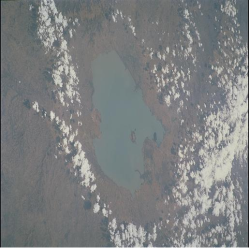
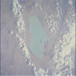
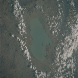
Figure 2: Images courtesy of the Image Science & Analysis Laboratory, NASA Johnson Space Center. For details see text.

Note that the lake’s border is rather fuzzy, resulting in a low image gradient. The output of edge detection algorithms is degraded even further by the substantial cloud cover. Therefore, the border was traced manually by a volunteer. The result is shown in the left-most panel in Figure 3. There are $73$ points along each border curve.

Figure 3: Left panel: Sampled boundary curves corresponding to Figure 2. Circles trace the boundary of Lake Tana in the left-most panel, triangles correspond to the middle panel, and crosses trace the lake boundary in the right-most panel of Figure 2. Right panel: Estimated border.

In contrast to the simulated data considered in the previous subsection, the curves are not necessarily well aligned. We therefore consider $M_{73}(\alpha_{0},\alpha_{1},\alpha_{2})$ as in (15). Using $20$ Fourier coefficients and $\alpha_{0}=0$, the optimal parameters are $\hat{\alpha}_{1}=-0.44$ and $\hat{\alpha}_{2}=-2.33$ radians. The value of the optimisation function is $1195.048$ corresponding to an average error of $2.34$ pixels. The result can be improved by including diffeomorphic changes in speed. Optimising $M_{73}(\alpha_{0},\alpha_{1},\alpha_{2},w_{0},w_{1},w_{t})$ for vectors $w_{t}$ in ${\mathbb{R}}^{2m}$ with $m=5$, cf. Section 4, we find an $M$-value of $568.0997$ corresponding to an average error of $1.61$ pixels. The optimal parameters are

$$\hat{w}_{1}=(0.032,0.029,0.037,0.015,0.0058,0.036,0.016,0.0096,-0.0080,0.021)^{T}$$

and

$$\hat{w}_{2}=(0.016,0.037,0.0081,-0.016,0.037,0.031,0.024,0.0064,0.047,0.029)^{T}$$

for the diffeomorphisms and $\hat{\alpha}_{1}=-0.42$ and $\hat{\alpha}_{2}=-2.32$. Finally, the estimated curve is plotted in the right-most panel in Figure 3.

6 Discussion

In this paper, we formulated a model for objects with uncertain boundaries using concepts from pattern theory in combination with cyclic Gaussian processes. The unknown boundary was estimated as a spectral mean by carrying out maximum likelihood estimation in the Fourier domain and transforming the results back to the spatial domain. We considered the integrated squared error and demonstrated how to deal with misalignment of the data. Finally, we applied the methods to simulated and real data.

The approach may be generalised to periodic change models. Indeed, write $\tau$ for the period. Then we may formulate the model

$$X_{j+t\tau}^{l}=X_{j+t\tau}(\theta_{l})=\Gamma^{(j)}(\varphi_{j+t\tau}(\theta_{l}-\alpha_{j+t\tau}))+N_{j+t\tau}^{(j)}(\varphi_{j+t\tau}(\theta_{l}-\alpha_{j+t\tau}))$$ (16)

for $t=0,1,\dots$. Here the $N^{(j)}$ are independent homogeneous mean zero cyclic Gaussian noise processes, the $\Gamma^{(j)}$ are unknown template curves at $j=0,\dots,\tau-1$ steps into the period. Since the data is periodic, (16) splits into $\tau$ submodels of the form discussed in this paper.

Finally, it is worth noting that, although they are prevalent in shape analysis [17], diffeomorphisms have not been studied much in stochastic geometry. In this paper, they have been used in different roles: for curve modelling and for alignment. It seems to the author that there is scope for further research concerning the modelling of random compact sets by means of their boundary curves in light of the Jordan–Schőnflies theorem [12].

References

• [1] Aletti, G. and Ruffini, M. (2013). Is the Brownian bridge a good noise model on the circle? Technical Report, ArXiv 1210.8245v2, May 2013.
• [2] Bigot, J. (2011). Fréchet means of curves for signal averaging and application to ECG data analysis. Research report, University of Toulouse.
• [3] Burrough, P. and Frank, A. (1996). Geographic objects with indeterminate boundaries. London: Taylor & Francis.
• [4] Chatfield, C. and Collins, A.J. (1980). Introduction to multivariate analysis. London: Chapman and Hall.
• [5] Coddington, E.A. and Levinson, N. (1955). Theory of ordinary differential equations. New York: McGraw–Hill.
• [6] Cramèr, H. and Leadbetter, M.R. (1967). Stationary and related stochastic processes. Sample function properties and their applications. New York: Wiley.
• [7] Dempster, A.P. (1967). Upper and lower probabilities induced by a multivalued mapping. Annals of Mathematical Statistics, 38:325–329.
• [8] Gohberg, I. and Goldberg, S. (1981). Basic operator theory. Boston: Birkha̋user.
• [9] Grenander, U. and Miller, M.I. (2007). Pattern theory: from representation to inference. Oxford: Oxford University Press.
• [10] Hobolth, A., Pedersen, J. and Jensen, E.B.V. (2003). A continuous parametric shape model. Annals of the Institute of Statistical Mathematics, 55:227–242.
• [11] Jónsdóttir, K.Y. and Vedel Jensen, E.B. (2005). Gaussian radial growth. Image Analysis and Stereology, 24:117–126.
• [12] Keren, D. (2004). Topologically faithful fitting of simple closed curves. IEEE Transactions on Pattern Analysis and Machine Intelligence, 26:118–123.
• [13] Molchanov, I.S. (2005). Theory of random sets. London: Springer.
• [14] Rogers, L.C.G. and Williams, D. (1994). Diffusions, Markov processes, and martingales. Volume One: Foundations. (Second edition). Chichester, Wiley.
• [15] Shafer, G. (1976). Mathematical theory of evidence. Princeton: Princeton University Press.
• [16] Soetaert, K., Petzoldt, T. and Woodrow Setzer, R. (2010). Solving differential equations in R: Package deSolve. Journal of Statistical Software, 33:1–25.
• [17] Younes, L. (2010). Shapes and diffeomorphisms. Berlin: Springer.
• [18] Zimmermann, H.-J. (2001). Fuzzy set theory and its applications. (Fourth edition). Dordrecht: Kluwer.