Theory of Antiferromagnetic Order in High-$T_{c}$ Oxides:
An Approach Based on Ginzburg-Landau Expansion

Abstract

The mean-field phase diagram of antiferromagnetic order in $t$-$J$ model has been examined, using the free energy obtained by Ginzburg-Landau (GL) expansion. We extended the usual GL theory in two ways: First, we have included higher order terms with respect to the spatial derivative (or wave number) to incorporate the incommensurate antiferromagnetic order. Second, we have also included higher order terms with respect to the order parameter amplitude, in order to treat the first order phase transition between paramagnetic and antiferromagnetic phase, which appears at some doping rates. We found the possibility of tricritical point and critical endpoint in the magnetic phase diagram of the high-$T_{c}$ oxides associated with the commensurate and incommensurate antiferromagnetic order. The possible effects of thermal fluctuations and randomness (spin glass) are also discussed qualitatively based on the GL free energy.

1 Introduction

From the early stage of the research of high-$T_{c}$ oxides, the magnetic structure of these materials has been considered as a key factor in understanding the mechanism of superconductivity. Until now, various intriguing results, both theoretical and experimental, have been obtained and the research is still going on. One of the most interesting phenomena may be the pseudogap, which has not been completely understood until now (see Refs. Timusk:1999wp,Norman:2005vr and references therein).

Among the various theoretical efforts to understand the mechanism of high-$T_{c}$ oxides, the $t$-$J$ model is one of the promising model to capture the natures of strong correlations [3, 4, 5, 6, 7]. The magnetic responses in NMR or neutron scattering experiments have been analyzed based on $t$-$J$ model [8, 9, 10]. The antiferromagnetic order has been also studied[11].

Recently, the synthesis of multilayered cuprates has revealed that the antiferromagnetic phase is more robust in multilayered materials [12, 13, 14] than single-layered ones [15, 16], thus suggesting the importance of dimensionality on the pseudogap and antiferromagnetism in high-$T_{c}$ oxides (see Ref. Mukuda:2011km and references therein). Several authors have studied the effects of interlayer coupling to understand these features from theoretical point of view [17, 18, 19, 20]. Another important aspect of the multilayered systems is the coexistence of superconductivity and antiferromagnetism in a certain region of the phase diagram [21, 22, 23]. Such phenomenon has been studied theoretically also using $t$-$J$ model [26, 24, 25, 27].

The researches to refine understanding of the $t$-$J$ model are also currently in progress. Recently, Yamase et al. have studied antiferromagnetic order in $t$-$J$ model incorporating the possibility of the incommensurate order[25]. It has been shown that the incommensurate antiferromagnetic (IC-AF) order can be stable in a certain range of doping in addition to the ordinary commensurate antiferromagnetic (C-AF) order which was first studied in Ref. Inaba:1996fm.

In this paper, we extend the study of Ref. Yamase:2011kf and re-examine the details of the magnetic phase diagram of $t$-$J$ model. Following the study by one of the present authors (KK) [27], we derive the Ginzburg-Landau (GL) free energy of antiferromagnetic order based on the $t$-$J$ model. We extend the GL free energy in the following two ways: Firstly, we introduce the higher order terms of gradient expansion of the order parameter. In the usual GL free energy, the spatial derivative (or the wave number $\vec{q}$ dependence) is kept only to the second order. However, the IC-AF order is the “finite-$\vec{q}$ antiferromagnetic order”and we need to keep higher order terms to treat it. Therefore, we keep up to the fourth order in $\vec{q}$. Secondly, the expansion with respect to the order parameter amplitude is also extended. Actually, we will find that the free energy as a function of the order parameter amplitude is strongly nonlinear and, in some case, the first order transition can occur. To incorporate these features, we include up to the sixth order in the amplitude, instead of the ordinary fourth-order expansion.

In order to concentrate on the antiferromagnetic order, we neglect the other orders such as RVB order. This treatment, although limited in quantitative accuracy, may be sufficient to capture the overall structure of the magnetic phase diagram of the high-$T_{c}$ oxides. For example, the antiferromagnetic phase transition lines obtained in this paper (Fig. 2 of this paper) qualitatively coincides with those obtained by Inaba et al. [11] and Yamase et al.[25]. also taking the RVB order into account (see especially Fig. 2 of Ref. Yamase:2011kf).

This paper is organized as follows: In Sect. 2, we describe the model and the method to derive GL free energy. In Sect. 3, basic feature of our nonlinear GL free energy is discussed. In Sect. 4, the magnetic phase diagram of the high-$T_{c}$ oxides is discussed based on the derived GL free energy. In Sect. 5, we summarize our results. Some calculations are given in the Appendices.

We adopt units $k_{B}=\hbar=1$ throughout.

2 Derivation of Ginzburg-Landau Free Energy

Here we derive the Ginzburg-Landau (GL) free energy which describes the antiferromagnetic order in high-$T_{c}$ oxides.

2.1 Model

We start from the Hamiltonian of the $t$-$J$ model,

$$H =-t\sum_{j,\sigma}\sum_{\hat{\delta}=\pm x,\pm y}\tilde{c}^{\dagger}_{j+\hat{\delta}\sigma}\tilde{c}_{j\sigma}+\frac{J}{2}\sum_{j}\sum_{\hat{\delta}=\pm\hat{x},\pm\hat{y}}\vec{S}_{j}\cdot\vec{S}_{j+\hat{\delta}}$$ (1)

where $t$ is the hopping integral, $J$ is the superexchange interaction and the double occupancy is assumed to be removed from the Fock space. We consider a simple square lattice, whose lattice sites are numbered by $j$, and $j+\hat{\delta}$ correspond to the nearest-neighbor sites of $j$. (In this paper, we consider the case of nearest-neighbor hopping only. ) Operator $\tilde{c}_{j\sigma}^{\dagger}$ ($\tilde{c}_{j\sigma}$) is the creation (annihilation) operator of an electron on the $j$-th site with spin $\sigma$ ($\sigma=\uparrow$ or $\downarrow$). Here we adopt the slave-boson method, in which an electron operator is decomposed as $\tilde{c}_{j\sigma}=b^{\dagger}_{j}f_{j\sigma}$, where $b^{\dagger}_{j}$ is the creation operator of a holon (boson) and $f_{j\sigma}$ in the annihilation operator of a spinon (fermion). The sum of holon number and spinon number on each site should be unity so that the double occupancy is absent. The spin operator is then given by $\vec{S}_{j}=(1/2)(f_{j\alpha}^{\dagger}\vec{\sigma}_{\alpha\beta}f_{j\beta})$, where $\alpha,\beta=\{\uparrow,\downarrow\}$ and $\vec{\sigma}_{\alpha\beta}$ are the Pauli matrices.

Next we introduce mean-field approximation[5]. Since we consider the region where the doping rate $\delta$ is sufficiently high ($\delta>0.14$), we assume that holons bose-condense at a higher temperature than the antiferromagnetic transition temperature, and put $\langle b_{j}^{\dagger}b_{k}\rangle=\langle b_{j}\rangle^{2}=\delta$ in the following. Here $\langle\cdots\rangle$ denotes statistical average. We also introduce the bond order parameter $\chi=2\langle f_{j\uparrow}^{\dagger}f_{j+\hat{\delta}\uparrow}\rangle=2\langle f_{j\downarrow}^{\dagger}f_{j+\hat{\delta}\downarrow}\rangle$, which is assumed to be spatially constant. Then the microscopic Hamiltonian for the “spinon”part, after decoupling the superexchange term, becomes $H=H_{0}+H_{I}$,

$$H_{0}= -\sum_{j,\sigma}\sum_{\hat{\delta}=\pm x,\pm y}\tilde{t}f_{j+\hat{\delta}\sigma}^{\dagger}f_{j\sigma}-\mu\sum_{j\sigma}f_{j\sigma}^{\dagger}f_{j\sigma}$$

$$H_{I}= J\sum_{j}\sum_{\hat{\delta}=\pm\hat{x},\pm\hat{y}}\left\langle\vec{S}_{j}\right\rangle\cdot\vec{S}_{j+\hat{\delta}}-\frac{J}{2}\sum_{j}\sum_{\hat{\delta}=\pm\hat{x},\pm\hat{y}}\left\langle\vec{S}_{j}\right\rangle\cdot\left\langle\vec{S}_{j+\hat{\delta}}\right\rangle$$ (2)

where $\mu$ is the chemical potential of spinons. The parameter $\tilde{t}$ is given by $\tilde{t}=t\delta+(3/8)J\chi$, where $\chi$ and $\mu$ are determined self-consistently from

$$\chi=\frac{1}{N}\sum_{\vec{k}}\gamma_{\vec{k}}f(\xi_{\vec{k}}),\,\,\,\delta=1-\frac{2}{N}\sum_{\vec{k}}f(\xi_{\vec{k}}).$$ (3)

Here $N$ is the total number of the lattice sites, $\gamma_{\vec{k}}=\cos k_{x}+\cos k_{y}$, $\xi_{\vec{k}}=-2\tilde{t}\gamma_{\vec{k}}-\mu$ and $f(z)=(1+e^{z/T})^{-1}$ with $T$ being the temperature. The Fourier transform is defined as $f_{\vec{k}}=\sqrt{N}^{-1}\sum_{j}f_{j}e^{-i\vec{k}\cdot\vec{r}_{j}}$, where $\vec{r}_{j}$ is the coordinate of the $j$-th lattice site and $\vec{k}$-sum is taken over the first Brillouin zone defined by $|k_{x}|,|k_{y}|<\pi$. In this paper we take the lattice spacing to be unity.

We introduce the order parameter $m_{j}$ by $\langle\vec{S}_{j}\rangle\equiv m_{j}\,\vec{n}_{j}$, where $\vec{n}_{j}$ is a unit vector. We assume that the spatial variation of $\vec{n}_{j}$ is so gradual that we can treat it as an adiabatic change for spinons. We take the quantization axis ($z$-axis) of the spins to be parallel to $\vec{n}_{j}$, and $m_{j}$ can be written as $\langle f_{j\uparrow}^{\dagger}f_{j\uparrow}-f_{j\downarrow}^{\dagger}f_{j\downarrow}\rangle/2$. Within this approximation, $H_{I}$ is given as

$$H_{I} =\frac{J}{2}\sum_{j}\sum_{\hat{\delta}=\pm\hat{x},\pm\hat{y}}m_{j+\hat{\delta}}(f_{j\uparrow}^{\dagger}f_{j\uparrow}-f_{j\downarrow}^{\dagger}f_{j\downarrow})$$

$$-\frac{J}{2}\sum_{j}\sum_{\hat{\delta}=\pm\hat{x},\pm\hat{y}}m_{j}m_{j+\hat{\delta}}.$$ (4)

Later, we will recover the vector degree of freedom of the spins at the GL level.

Throughout this paper, we take $J$ to be the unit of energy and put $t=4J$.

2.2 Perturbative Expansion

Using path-integral framework, the free energy is obtained as follows: We write the partition function as,

$$Z =\int{\cal D}[f_{\vec{k}\omega_{n}\sigma}^{*},f_{\vec{k}\omega_{n}\sigma}]e^{-S-S_{0}}$$

$$S =-\sum_{\omega_{n},\vec{k},\vec{k}^{\prime},\sigma}\left[G_{\vec{k},\omega_{n}}^{-1}\delta_{\vec{k},\vec{k}^{\prime}}-\frac{(-1)^{\sigma}}{\sqrt{N}}J\gamma_{\vec{k}-\vec{k}^{\prime}}m_{\vec{k}-\vec{k}^{\prime}}\right]f_{\vec{k}\omega_{n}\sigma}^{*}f_{\vec{k}^{\prime}\omega_{n}\sigma}$$

$$=-\sum_{\omega_{n},\sigma}{}^{t}\vec{f}_{\omega_{n}\sigma}^{*}\cdot\left[\hat{G}^{-1}+\frac{(-1)^{\sigma}}{\sqrt{N}}\hat{\Gamma}\right]\cdot\vec{f}_{\omega_{n}\sigma}$$ (5)

where $G_{\vec{k},\omega_{n}}=(i\omega_{n}-\xi_{\vec{k}})^{-1}$ with $\omega_{n}=(2n+1)\pi T$ being the Matsubara frequency, and $(-1)^{\sigma}=1$ $(-1)$ for $\sigma=\uparrow$ ($\downarrow$). The constant $S_{0}$ is given by $-T^{-1}\sum_{\vec{q}}J\gamma_{\vec{q}}|m_{\vec{q}}|^{2}$. In the last line, we used the matrix representation for indices $\vec{k}$ and $\vec{k}^{\prime}$, where

$$\left\{\hat{G}\right\}_{\vec{k},\vec{k}^{\prime}}=G_{\vec{k},\omega_{n}}\delta_{\vec{k},\vec{k}^{\prime}},\,\,\,\left\{\hat{\Gamma}\right\}_{\vec{k},\vec{k}^{\prime}}=-J\gamma_{\vec{k}-\vec{k}^{\prime}}m_{\vec{k}-\vec{k}^{\prime}}.$$ (6)

The free energy is, then, expressed as

$$F =-T\sum_{\omega_{n},\sigma}\left\{{\rm Tr}\ln\left(\hat{G}^{-1}+\frac{(-1)^{\sigma}}{\sqrt{N}}\hat{\Gamma}\right)\right\}+TS_{0}$$

$$=-T\sum_{\omega_{n},\sigma}{\rm Tr}\left\{\ln\hat{G}^{-1}+\sum_{l=1}^{\infty}\frac{(-1)^{l-1}}{l}\left(\frac{(-1)^{\sigma}\hat{G}\,\hat{\Gamma}}{\sqrt{N}}\right)^{l}\right\}+TS_{0}.$$ (7)

From this equation the second order term in $m_{\vec{q}}$ is given by

$$F^{(2)} =\sum_{\vec{q}}\left(-J\gamma_{\vec{q}}+J^{2}T\gamma_{\vec{q}}^{2}\sum_{\vec{k},\omega_{n}}G_{\vec{k},\omega_{n}}G_{\vec{k}-\vec{q},\omega_{n}}\right)|m_{\vec{q}}|^{2}$$ (8)

$$=\sum_{\vec{q}}\,\,J\,\gamma_{\vec{q}}\,(1-J\,\gamma_{\vec{q}}\,\chi^{(0)}_{\vec{q}})|M_{\vec{q}}|^{2}.$$ (9)

Here we have substituted $\vec{q}\rightarrow\vec{q}+\vec{Q}$ where $\vec{Q}=(\pi,\pi)$ is the reciprocal lattice vector (Note the relation $\gamma_{\vec{q}+\vec{Q}}=-\gamma_{\vec{q}}$. ), and introduced the staggered (antiferromagnetic) order parameter $M_{j}\equiv m_{j}e^{i\vec{Q}\cdot\vec{r}_{j}}$ (or $M_{\vec{q}}\equiv m_{\vec{q}+\vec{Q}}$). The bare staggered susceptibility $\chi^{(0)}_{\vec{q}}$ is given by

$$\chi^{(0)}_{\vec{q}} =-\frac{T}{N}\sum_{\vec{k},\omega_{n}}G_{\vec{k},\omega_{n}}G_{\vec{k}-\vec{q}-\vec{Q},\omega_{n}}=-\frac{1}{N}\sum_{\vec{k}}\,\,\frac{f(\xi_{\vec{k}})-f(\xi_{\vec{k}-\vec{Q}-\vec{q}})}{\xi_{\vec{k}}-\xi_{\vec{k}-\vec{Q}-\vec{q}}}.$$ (10)

The free energy $F^{(2)}$ is expanded with respect to $\vec{q}$ up to the fourth order. From the symmetry argument, the terms appearing in this expansion are proportional to $1$, $|\vec{q}|^{2}$, $q_{x}^{4}+q_{y}^{4}$, or $q_{x}^{2}q_{y}^{2}$.

The higher order terms with respect to the amplitude $|M_{j}|$ can be derived from the following free energy $U$, which is obtained by assuming that the order parameter is constant, $M_{j}=M$ (see Appendix B),

$$U(M)=2JM^{2}$$

$$-\frac{2T}{N}\sum_{\vec{k}\in{\rm MBZ}}\left[\ln\left(2\cosh\frac{E_{\vec{k}}-\mu}{2T}\right)+\ln\left(2\cosh\frac{E_{\vec{k}}+\mu}{2T}\right)\right]$$ (11)

where $E_{\vec{k}}=\sqrt{(2\tilde{t}\gamma_{\vec{k}})^{2}+(2JM)^{2}}$. In this case, the range of $\vec{k}$-sum is the magnetic Brillouin zone (MBZ), defined by $|k_{x}|+|k_{y}|\leq\pi$.

The total free energy is expressed as $F=F^{(2)}+\sum_{j}\bar{U}(M_{j})$, where $\bar{U}(M)=\beta_{4}M^{4}+\beta_{6}M^{6}+\cdots$ is obtained by removing the second order term from the series expansion of $U(M)$ with respect to $M$, since the second order term is already included in $F^{(2)}$. Here the constant part independent of $M$ is suppressed.

3 Extension of the GL Expansion

We assume the form of our GL free energy to be

$$F=\sum_{\vec{q}}K(\vec{q})|M_{\vec{q}}|^{2}+\sum_{j}\left\{\beta_{4}M_{j}^{4}+\beta_{6}M_{j}^{6}\right\},$$ (12)

where the wave vector dependence of $K(\vec{q})$ is given by

$$K(\vec{q}) =A+B|\vec{q}|^{2}+C_{1}(q_{x}^{4}+q_{y}^{4})+C_{2}q_{x}^{2}q_{y}^{2}.$$ (13)

The coefficients $\beta_{4}$ and $\beta_{6}$ are defined in the previous section, and the calculation of $A$, $B$, $C_{1}$ and $C_{2}$ is given in Appendix A. Note that all the coefficients depend on $T$ and $\delta$.

3.1 GL coefficients

Here we discuss the behavior of GL coefficients. In this paper we concentrate on the region ($0.14<\delta<0.18$ and $0.03<T<0.25$) depicted in Fig. 1 (color online), since the IC-AF order is most significant in this region. Unfortunately, whole of this region can not be covered by the present treatment. The reason is as follows:

1. In order for the $F$ in Eq. (12) to be stable as a function of the amplitude $M_{j}$, at least the highest order term in $M_{j}$ should be positive. In the present case, $\beta_{6}>0$ is required. However, this is not fulfilled in the whole region; the boundary between the regions of $\beta_{6}>0$ and $\beta_{6}<0$ is shown by dashed-dotted line in Fig. 1.

2. As for the $\vec{q}$-dependence in $K(\vec{q})$, the highest order term should be also positive. Otherwise, the higher order terms, e.g.$q_{x}^{6}+q_{y}^{6}$, may not be negligible. This condition is given by $C_{1}>0$ for $C_{2}-2C_{1}>0$ and $C_{1}+C_{2}>0$ for $C_{2}-2C_{1}<0$ (see the next section for details). In Fig. 1, we have depicted the boundary between $C_{1}>0$ and $C_{1}<0$ (dashed line). The value $C_{1}+C_{2}$ is always positive in the area of $C_{1}>0$[28].

From the above considerations, we conclude that the present approach is valid in the painted region (in yellow) in Fig. 1. In the same figure, we have also shown the lines corresponding to the previously obtained results. The line indicated by “Inaba et al., 1996”, is the line at which instability to C-AF order occurs[11]. Within our theory, this corresponds to the line “$A=0$”. The line indicated by “Yamase et al., 2011”, is obtained as the line at which $K(\vec{q})$ becomes negative for a certain $\vec{q}$[25, 29].

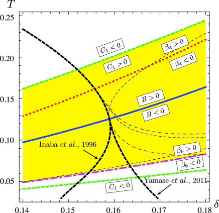
Figure 1: (Color online) Map of the GL coefficients: sign changes of GL coefficients are indicated in the figure. Bold dashed lines correspond to previously obtained results, by Inaba et al.[11] and Yamase et al. [25] Thin broken lines are shown to clarify the correspondence with Fig. 2. The painted area (in yellow) is the region where the present GL expansion is well-defined.

3.2 Incommensurate Antiferromagnetic Order

Let us examine the possible antiferromagnetic order based on $F^{(2)}$. In contrast to the ordinary GL free energy, the quadratic coefficient $B$ can be either positive or negative. In case of $B>0$, the free-energy minimum as a function of the wave vector $\vec{q}$ is located at the origin $\vec{q}=0$ and the corresponding order is C-AF. In case of $B<0$, the free-energy minima appear at non-zero $\vec{q}$ and incommensurate order becomes stable. In the latter case, we have two situations. Let us put $q_{x}=q\cos\theta$, $q_{y}=q\sin\theta$. Then $K(\vec{q})$ becomes

$$K(q,\theta) =A+Bq^{2}+q^{4}\left(C_{1}+C^{\prime}_{2}\cos^{2}\theta\sin^{2}\theta\right),$$

$$=A+Bq^{2}+q^{4}\left(C_{1}+C^{\prime}_{2}\frac{1-\cos 4\theta}{8}\right),$$ (14)

where $C^{\prime}_{2}=C_{2}-2C_{1}$.

In case of $C^{\prime}_{2}>0$, the minima of $K(q,\theta)$ as a function of $\theta$ lie at $\theta=\theta_{n}\equiv n\pi/2$ ($n$: integer) and

$$K\left(q,\theta_{n}\right) =C_{1}\left(q^{2}+\frac{B}{2C_{1}}\right)^{2}-\frac{B^{2}}{4C_{1}}+A.$$ (15)

$K(\vec{q})$ takes minimum at $q=q_{\rm min}\equiv\sqrt{|B|/(2C_{1})}$. We call this order “IC₁-AF”.

In case of $C^{\prime}_{2}<0$, the minima of $K(q,\theta)$ lie at $\theta=\theta^{\prime}_{n}\equiv(2n+1)\pi/4$ and

$$K\left(q,\theta^{\prime}_{n}\right) =\lambda\left(q^{2}+\frac{B}{2\lambda}\right)^{2}-\frac{B^{2}}{4\lambda}+A$$ (16)

where $\lambda=(C_{1}+C_{2})/2$. $K(\vec{q})$ takes minimum at $q=q_{\rm min}\equiv\sqrt{|B|/(2\lambda)}$. We call this order “IC₂-AF”.

The positions of minima in $\vec{q}$-space are shown in the inset of Fig. 3 (color online).

3.3 The First Order Phase Transition

In order to estimate the free energy including IC-AF, we restore the vector degrees of freedom of the order parameter, namely $M_{j}\rightarrow M_{j}\vec{n}_{j}\equiv\vec{M}_{j}$. Then the free energy can be written as

$$F=\sum_{\vec{q}}K(\vec{q})|\vec{M}_{\vec{q}}|^{2}+\sum_{j}\left\{\beta_{4}|\vec{M}_{j}|^{4}+\beta_{6}|\vec{M}_{j}|^{6}\right\}.$$ (17)

We take the wave vector of the incommensurate order to be parallel to $x$-axis, and put the order parameter as

$$\vec{M}_{j}=(M\cos qx_{j},M\sin qx_{j},0),$$ (18)

where $\vec{r}_{j}=(x_{j},y_{j})$. Note that if we take the order parameter to be unidirectional, such as $\vec{M}_{j}=(M\cos qx_{j},0,0)$, the amplitude $|\vec{M}_{j}|$ changes spatially, thus causing a free energy loss. Therefore, Eq. (18), whose magnitude is constant, may be most stable. The free energy corresponding to this order parameter is given by

$$F=N\left\{K(q)M^{2}+\beta_{4}M^{4}+\beta_{6}M^{6}\right\}.$$ (19)

Next, we minimize the free energy with respect to $M$. In case of $\beta_{4}>0$, we obtain the ordinary second order phase transition. However, in case of $\beta_{4}<0$, the first order phase transition occurs:

1. In case of $K(q_{\rm min})>|\beta_{4}|^{2}/(3\beta_{6})$, $F$ is a monotonic function of $M$ and always $M=0$ is stable.

2. In case of $|\beta_{4}|^{2}/(3\beta_{6})>K(q_{\rm min})>|\beta_{4}|^{2}/(4\beta_{6})$, $F$ has metastable states, although $M=0$ is still stable.

3. In case of $|\beta_{4}|^{2}/(4\beta_{6})>K(q_{\rm min})>0$, non-zero $M$ becomes stable, although $M=0$ is still metastable. In the ordered state the free energy takes the value,

   $$F=-\frac{\left(-\beta_{4}+\sqrt{\beta_{4}^{2}-3k\beta_{6}}\right)^{2}\left(\beta_{4}+2\sqrt{\beta_{4}^{2}-3k\beta_{6}}\right)}{27\beta_{6}^{2}},$$ (20)

   where $k=K(q_{\rm min})$.

4. In case of $0>K(q_{\rm min})$, $M=0$ becomes unstable and only the ordered state is stable.

As seen from the above, the system undergoes the first order phase transition at the temperature defined by $|\beta_{4}|^{2}/(4\beta_{6})=K(q_{\rm min})$.

4 Mean Field Phase Diagram

Now we are ready to discuss the mean-field phase diagram. From the arguments given above, we found several phases shown in Fig. 2 (color online).

In contrast to the preceding results[25], where the existence of IC-AF is pointed out between “Inaba et al.”-line and “Yamase et al.”-line in Fig. 1, we found a significantly large region of IC-AF in Fig. 2. (IC-AF region is divided into IC₁-AF and IC₂-AF. However we do not consider the result of the IC₂-AF is completely reliable, since GL expansion is not good in this region. Therefore we do not take this phase seriously in this paper. ) Though the present treatment is not applicable in the hatched region, C-AF phase may be occupying this region also.

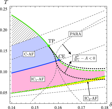
Figure 2: (Color online) Phase diagram obtained by the present analysis. Bold solid (green) line shows the second order phase transition and bold dashed line (green) shows that of first order. PARA is the paramagnetic phase. IC₁-AF and IC₂-AF are incommensurate antiferromagnetic phase, with different incommensurate wave vectors (see Fig.3 for detail), and bold dashed-dotted line (green) is the boundary between them. Thin broken lines are the reproduction of those shown in Fig. 1. The area between two dotted lines (black) is the region where metastable states associated with the first order phase transition exist. TP is the tricritical point and CE is the critical endpoint.

Next we discuss the nature of the phase transitions. We found a first order transition line, shown by the bold dashed line (green) in Fig. 2. This line is defined by $K(q_{\rm min})=|\beta_{4}|^{2}/(4\beta_{6})$, which corresponds to the temperature at which the free energy of Eq. (20) becomes negative, namely smaller than the free energy of the paramagnetic state $M=0$. This first-order-transition line extends up to $\beta_{4}=0$ line (see Fig. 1) and is connected to the second-order-transition line in the region of $\beta_{4}>0$. This connecting point, indicated by TP in Fig. 2, is called the tricritical point [30]. Two dotted lines (black) are defined by $|\beta_{4}|^{2}/(3\beta_{6})=K(q_{\rm min})$ (upper line) and $B^{2}/(4C_{1})-A=0$ (lower line). In the region between these two lines, metastable states exist. We can estimate the strength of the first order phase transition, following Ref. Halperin:1974vx, by the width of the temperature region, where the metastable states exist. In our case, the first-order nature is stronger in the PARA to IC₁-AF transition and weaker in the PARA to C-AF transition. The lower dotted line shows the temperature below which $K(\vec{q})$ becomes negative at a certain $\vec{q}$. Therefore this line corresponds to the phase transition line obtained by Yamase et al.[25] (shown in Fig. 1). Comparing these lines, we can see that GL expansion is overestimating the transition temperature as compared to the study by Yamase et al., obtained by treating exact $\vec{q}$-dependence of $K(\vec{q})$, especially at higher doping region ($\delta>0.16$).

Finally we study the phase transition between C-AF and IC-AF. In Fig. 3 we have plotted the free energy of C-AF state ($\vec{q}=0$) and IC-AF state ($\vec{q}=(q_{\rm min},0)$) along the line $\delta=0.15$. The wave number $q_{\rm min}$ is also shown in a same plane. The solid curve (IC₁-AF, in red) becomes lower than dashed curve (C-AF, in blue) at the temperature below $T\sim 0.112$, and the connection between two curves seems to be smooth. This probably suggests the second order phase transition between C-AF and IC-AF phase. Therefore the intersection of the C-IC boundary and the first-order-transition line, namely CE in Fig. 2, is the so-called critical endpoint, at which the second-order-transition line ends at the first-order-transition line[30].

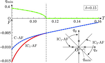
Figure 3: (Color online) Plot of the free energy of C-AF and IC-AF states as a function of temperature at $\delta=0.15$. The development of the incommensurate wave number $q_{\rm min}$ in the IC-AF phase is also shown in the upper graph. The inset shows the locations of incommensurate wave vectors in IC₁-AF state. In case of IC₂-AF state the positions are rotated by 45^∘ around the origin.

5 Discussion

In this paper we have clarified the mean-field magnetic phase diagram of the $t$-$J$ model within the GL approximation. Obtained phase diagram contains a significantly large area of IC-AF phase, as compared to the previous theories[11, 25]. At this stage, these findings may not have direct relationships to the experimentally obtained phase diagram[12, 14]. However they include several clues to the quantitative understanding of the high-$T_{c}$ oxides based on $t$-$J$ model.

Firstly, our results provide an insight into the effects of the thermal fluctuations in high-$T_{c}$ oxides. In the conventional GL free energy, the quadratic coefficient as a function of wave number is assumed to be constant near the critical points. In our free energy, $\vec{q}$-dependence of $K(\vec{q})$ is more complicated. Especially, at the boundary between C-AF and IC-AF, the quadratic coefficient $B$ vanishes, which may cause a significant enhancement of the fluctuation effects. There is a possibility that C-AF area is strongly reduced in the phase diagram if we take into account the thermal fluctuations. Further research is ongoing in this direction. It may be also interesting to pursue possibilities of understanding pseudogap phase in relation to antiferromagnetic fluctuations, although in this case RVB order cannot probably be neglected.

Another important issue may be the existence of widely spread IC-AF phase. We may consider that this phase has some relationship with the experimentally observed “spin glass”in high-$T_{c}$ oxides[14]. The most important difference between C-AF and IC-AF phase is that multiple stable states, namely $\vec{q}=(\pm q_{\rm min},0)$ or $(0,\pm q_{\rm min})$, exist only in the latter phase (see the inset of Fig. 3). In the presence of randomness, there can exist domains of IC-AF orders with different $\vec{q}$ ’s and such a behavior is similar to spin glass system. Actually our GL free energy is similar to that discussed by Sherrington[32] in relation to the spin glass. According to that literature, the non-trivial $\vec{q}$-dependence (or the frustration) is crucial for the appearance of the spin glass order[32, 33]. It is also interesting that Yamase et al. has pointed out the relation between IC-AF to charge stripes[34]. Although it is just a possibility at this stage, the relation of IC-AF phase to experimentally observed spin glass phase and the charge stripes may be worth further studies.

6 Summary

We have examined the antiferromagnetic phase diagram of high-$T_{c}$ oxides based on $t$-$J$ model and GL expansion. It has been found that the incommensurate antiferromagnetic phase occupy larger area in the phase diagram than the preceding works[11, 25], and the transition from paramagnetic to antiferromagnetic (commensurate or incommensurate) phase can be first order depending on the doping. Possibilities of tricritical point and critical endpoint in the magnetic phase diagram are pointed out. Existence of the incommensurate antiferromagnetic phase may enhance the effects of thermal fluctuations and it may also lead to glass-like behavior in the presence of randomness.

This work was supported by JSPS KAKENHI Grant Numbers 24540392, 22540329.

Appendix A GL coefficients: $\vec{q}$-dependences

We calculate the quadratic GL coefficient $K(\vec{q})$ to the fourth order in the wave vector $\vec{q}$. This process can be carried out by applying Taylor series expansion with respect to $\vec{q}$ and performing the $\vec{k}$-summation over the Brillouin zone ($|k_{x}|,|k_{y}|<\pi)$ in Eq. (9). Basically this summation (integral) is not singular, however, if we expand it with respect to the wave numbers, $q_{x}$ and $q_{y}$, removable singularities (such as “0/0”) appear on the lines $|k_{x}|+|k_{y}|=\pi$. In the numerical calculation, this type of singularity also causes errors. To avoid this, it is advantageous to introduce the new coordinates $(k_{s},k_{t})$ by $k_{x}=(k_{s}+k_{t})/\sqrt{2}$, $k_{y}=(k_{s}-k_{t})/\sqrt{2}$. Then the lines $|k_{x}|+|k_{y}|=\pi$ become parallel (or perpendicular) to the axes. In this coordinate, $\xi_{\vec{k}}=-4\tilde{t}\cos(k_{s}/\sqrt{2})\cos(k_{t}/\sqrt{2})-\mu$, and the vector $\vec{Q}$ becomes $(0,\sqrt{2}\pi)$. We further introduce

$$\eta_{\vec{k}} =8\tilde{t}\cos(k_{s}/\sqrt{2})\cos(k_{t}/\sqrt{2}),$$

$$\delta\xi_{\vec{k},\vec{q}} =\xi_{\vec{k}+\vec{Q}+\vec{q}}-\xi_{\vec{k}+\vec{Q}}.$$ (21)

Then we obtain

$$\xi_{\vec{k}+\vec{Q}} =\xi_{\vec{k}}+\eta_{\vec{k}},$$

$$\xi_{\vec{k}+\vec{Q}+\vec{q}}-\xi_{\vec{k}} =\xi_{\vec{k}+\vec{Q}+\vec{q}}-\xi_{\vec{k}+\vec{Q}}+(\xi_{\vec{k}+\vec{Q}}-\xi_{\vec{k}})$$

$$=\delta\xi_{\vec{k},\vec{q}}+\eta_{\vec{k}},$$ (22)

and

$$\chi^{(0)}(\vec{q})=\frac{1}{N}\sum_{\vec{k}\in{\rm BZ}}\frac{\tanh(\beta(\xi+\eta+\delta\xi)/2)-\tanh(\beta\xi/2)}{\eta+\delta\xi},$$ (23)

where we have suppressed the arguments $\vec{k}$ and $\vec{q}$. Since all the $\vec{q}$ dependences are contained in $\delta\xi$, we first expand Eq. (23) with respect to $\delta\xi$ and, then, expand $\delta\xi$ with respect to $\vec{q}$. Note that, because $\delta\xi$ is the first order or higher in $q_{s}$ or $q_{t}$, the expansion up to the fourth order in $\delta\xi$ is sufficient for our purpose. Let us write

$$\chi^{(0)}(\vec{q})= \frac{1}{2N}\sum_{\vec{k}\in{\rm BZ}}\sum_{n=0}^{4}\alpha^{(n)}(\vec{k})(\delta\xi)^{n},$$ (24)

$$(\delta\xi)^{n}= \nu_{a}^{(n)}(\vec{k})+\nu_{b}^{(n)}(\vec{k})(q_{s}^{2}+q_{t}^{2})$$

$$\phantom{aaa}+\nu_{c1}^{(n)}(\vec{k})(q_{s}^{4}+q_{t}^{4})+\nu_{c2}^{(n)}(\vec{k})q_{s}^{2}q_{t}^{2},$$ (25)

where $\alpha^{(n)}(\vec{k})$ is the expansion coefficient of the $n$-th order, then $\chi^{(0)}(\vec{q})$ reads,

$$\chi^{(0)}(\vec{q})=c_{a}+c_{b}(q_{s}^{2}+q_{t}^{2})+c_{c1}(q_{s}^{4}+q_{t}^{4})+c_{c2}q_{s}^{2}q_{t}^{2}$$ (26)

with

$$c_{a}= \frac{1}{8\pi^{2}}\frac{1}{N}\sum_{\vec{k}\in{\rm BZ}}\sum_{n=0}^{4}\alpha^{(n)}(\vec{k})\nu_{a}^{(n)}(\vec{k})$$

$$= \frac{1}{8\pi^{2}}\frac{1}{N}\sum_{\vec{k}\in{\rm BZ}}\,\vec{\alpha}(\vec{k})\cdot\vec{\nu_{a}}(\vec{k}),\,\,\,\cdots,{\rm etc.},$$ (27)

where $\vec{\alpha}$ and $\vec{\nu}_{a}$ are five dimensional vector whose $n$-th component being $\alpha^{(n)}$ and $\nu^{(n)}_{a}$, respectively. By using the abbreviations,

$$C_{s} =\cos\left({{k_{s}}}/{\sqrt{2}}\right),C_{t}=\cos\left({{k_{t}}}/{\sqrt{2}}\right),$$

$$S_{s} =\sin\left({{k_{s}}}/{\sqrt{2}}\right),S_{t}=\sin\left({{k_{t}}}/{\sqrt{2}}\right),$$

$$C^{\prime}_{s} =\cos\left({\sqrt{2}}{{k_{s}}}\right),C^{\prime}_{t}=\cos\left({\sqrt{2}}{{k_{t}}}\right),$$

$$S^{\prime}_{s} =\sin\left({\sqrt{2}}{{k_{s}}}\right),S^{\prime}_{t}=\sin\left({\sqrt{2}}{{k_{t}}}\right),$$ (28)

the vector $\vec{\nu}_{a},\,\cdots$, etc. are given by

$$\vec{\nu}_{a}=(\nu_{a}^{(0)},\cdots,\nu_{a}^{(4)})=(1,0,0,0,0),$$ (29)

$$\vec{\nu}_{b}=\left(0,-{\tilde{t}}{C_{s}}{C_{t}},-2{\tilde{t}}^{2}({C^{\prime}_{s}}{C^{\prime}_{t}}-1),0,0\right),$$ (30)

$$\vec{\nu}_{c1}=\biggl{(}0,\frac{{\tilde{t}}{C_{s}}{C_{t}}}{24},\frac{1}{12}{\tilde{t}}^{2}\left\{{C^{\prime}_{s}}(7{C^{\prime}_{t}}+3)+3{C^{\prime}_{t}}-1\right\},$$

$$\phantom{aaaa}6{\tilde{t}}^{3}{C_{s}}{C_{t}}({C^{\prime}_{s}}{C^{\prime}_{t}}-1),32{\tilde{t}}^{4}\left({C_{s}}^{4}{S_{t}}^{4}+{C_{t}}^{4}{S_{s}}^{4}\right)\biggr{)},$$ (31)

$$\vec{\nu}_{c2}=\biggl{(}0,\frac{{\tilde{t}}{C_{s}}{C_{t}}}{4},\frac{1}{2}\tilde{t}^{2}\left\{{C^{\prime}_{s}}(7{C^{\prime}_{t}}-1)-{C^{\prime}_{t}}-1\right\},$$

$$\phantom{aaa}12{\tilde{t}}^{3}{C_{s}}{C_{t}}\left\{{C^{\prime}_{s}}(3{C^{\prime}_{t}}-2)-2{C^{\prime}_{t}}+1\right\},24\tilde{t}^{4}{S^{\prime}_{s}}^{2}{S^{\prime}_{t}}^{2}\biggr{)}.$$ (32)

The vector $\vec{\alpha}$ is given, using $\tau_{\pm}=\tanh\left\{(\eta\pm 2\mu)/(4{T})\right\}$, as

$$\vec{\alpha}=\biggl{(} \frac{{\tau_{+}}+{\tau_{-}}}{8\pi^{2}\eta},\frac{-\eta{\tau_{-}}^{2}+\eta-2{T}({\tau_{+}}+{\tau_{-}})}{16\pi^{2}\eta^{2}{T}},$$

$$\frac{\eta^{2}{\tau_{-}}\left({\tau_{-}}^{2}-1\right)+2\eta{T}\left({\tau_{-}}^{2}-1\right)+4T^{2}({\tau_{+}}+{\tau_{-}})}{32\pi^{2}\eta^{3}T^{2}},$$

$$\frac{1}{192\pi^{2}\eta^{4}T^{3}}\biggl{\{}\eta^{3}\left(-3{\tau_{-}}^{4}+4{\tau_{-}}^{2}-1\right)$$

$$\phantom{aaaaa}-6\eta^{2}{T}{\tau_{-}}\left({\tau_{-}}^{2}-1\right)-12\eta T^{2}\left({\tau_{-}}^{2}-1\right)$$

$$\phantom{aaaaaaaaaaa}-24T^{3}({\tau_{+}}+{\tau_{-}})\biggr{\}},$$

$$\frac{1}{384\pi^{2}\eta^{5}T^{4}}\biggl{\{}\eta^{4}{\tau_{-}}\left(3{\tau_{-}}^{4}-5{\tau_{-}}^{2}+2\right)$$

$$\phantom{aaaaa}+2\eta^{3}{T}\left(3{\tau_{-}}^{4}-4{\tau_{-}}^{2}+1\right)$$

$$\phantom{aaaaa}+12\eta^{2}T^{2}{\tau_{-}}\left({\tau_{-}}^{2}-1\right)+24\eta T^{3}\left({\tau_{-}}^{2}-1\right)$$

$$\phantom{aaaaa}+48T^{4}({\tau_{+}}+{\tau_{-}})\biggr{\}}\biggr{)}.$$ (33)

Since $\eta$ vanishes on the lines $|k_{x}|+|k_{y}|=\pi$ ($k_{s},k_{t}=\pm\pi/\sqrt{2}$), $\vec{\alpha}$ seems to diverge on these lines due to the powers of $\eta$ in the denominators. This is just superficial, because the numerators also vanish on the same lines. To avoid this singularity, we use Taylor series expansion with respect to $k_{s}$ and $k_{t}$ in the narrow region near the lines $|k_{x}|+|k_{y}|=\pi$, instead of using the original expression, Eq. (33).

From Eqs.(9) and (26), the GL coefficients in Eq. (13) are given by

$$A =J(1-2Jc_{a}),$$ (34)

$$B =-J^{2}\left(\frac{c_{a}}{2}-2c_{b}\right),$$ (35)

$$C_{1} =J^{2}\left(\frac{c_{a}}{24}-\frac{c_{b}}{2}+2c_{c1}\right),$$ (36)

$$C_{2} =-J^{2}\left(-c_{b}+2c_{c2}\right).$$ (37)

Appendix B GL coefficients: higher order in $M_{j}$

If the order parameter $M_{j}$ is a constant $M$, the Hamiltonian, Eqs. (2) and (4), is rewritten by limiting the summation with respect to $\vec{k}$ from the original Brillouin zone ($|k_{x}|$,$|k_{y}|<\pi$) to the magnetic Brillouin zone (MBZ) ($|k_{x}|+|k_{y}|<\pi$) as

$$H= \sum_{\sigma,\vec{k}\in{\rm MBZ}}\left(\begin{array}[]{c c}f_{\vec{k}\,\sigma}^{\dagger}&f_{\vec{k}-\vec{Q}\,\sigma}^{\dagger}\end{array}\right)\cdot$$ (39)

$$\left(\begin{array}[]{cc}\xi_{\vec{k}}&-iJ(-1)^{\sigma}M\\ -iJ(-1)^{\sigma}M&\xi_{\vec{k}-\vec{Q}}\end{array}\right)\cdot\left(\begin{array}[]{l}f_{\vec{k}\,\sigma}\\ f_{\vec{k}-\vec{Q}\,\sigma}\end{array}\right)+2JM^{2}.$$ (44)

Since $\xi_{\vec{k}}=-2\tilde{t}\gamma_{\vec{k}}-\mu$ and $\xi_{\vec{k}-\vec{Q}}=2\tilde{t}\gamma_{\vec{k}}-\mu$, we obtain the quasiparticle energy as

$$E=\pm\sqrt{(2\tilde{t}\gamma_{\vec{k}})^{2}+(2JM)^{2}}-\mu\equiv\pm E_{\vec{k}}-\mu.$$ (45)

Then the partition function is obtained following the ordinary recipe as,

$$Z=\prod_{\vec{k}\in{\rm MBZ}}\left\{(1+e^{-(E_{\vec{k}}-\mu)/T})(1+e^{(E_{\vec{k}}+\mu)/T})\right\}^{2}e^{-2JM^{2}/T}$$ (46)

and the free energy (or potential of $M$) is obtained by $U(M)=-T\ln Z$. The same formulae are given in Ref Yamase:2011kf.

References

• [1] T. Timusk and B. Statt: Rep. Prog. Phys. 62 (1999) 61.
• [2] M. R. Norman, D. Pines, and C. Kallin, Advances in Physics 54 (2005) 715.
• [3] P. W. Anderson: Science 235 (1987) 1196.
• [4] Z. Zou and P. W. Anderson: Phys. Rev. B 37 (1988) 627.
• [5] Y. Suzumura, Y. Hasegawa, and H. Fukuyama: J. Phys. Soc. Jpn. 57 (1988) 401.
• [6] N. Nagaosa and P. A. Lee: Phys. Rev. Lett. 64 (1990) 2450.
• [7] P. A. Lee and N. Nagaosa: Phys. Rev. B 46 (1992) 5621.
• [8] T. Tanamoto, K. Kuboki, and H. Fukuyama: J. Phys. Soc. Jpn. 60 (1991) 3072.
• [9] T. Tanamoto, H. Kohno, and H. Fukuyama: J. Phys. Soc. Jpn. 62 (1993) 717.
• [10] T. Tanamoto, H. Kohno, and H. Fukuyama: J. Phys. Soc. Jpn. 63 (1994) 2739.
• [11] M. Inaba, H. Matsukawa, M. Saitoh, and H. Fukuyama: Physica C 257 (1996) 299.
• [12] M. Julien: Physica B 329-333 (2003) 693.
• [13] Y. Kitaoka, H. Mukuda, S. Shimizu, S. Tabata, P. Shirage, and A. Iyo: J. Phys. Chem. Solids 72 (2011) 486.
• [14] H. Mukuda, S. Shimizu, A. Iyo, and Y. Kitaoka: J. Phys. Soc. Jpn. 81 (2011) 011008.
• [15] S. Sanna, G. Allodi, G. Concas, A. D. Hillier, and R. D. Renzi: Phys. Rev. Lett. 93 (2004) 207001.
• [16] A. Iyo, Y. Tanaka, H. Kito, Y. Kodama, P. Shirage, D. D. Shivagan, H. Matsuhata, K. Tokiwa, and T. Watanabe: J. Phys. Soc. Jpn. 76 (2007) 094711.
• [17] S. Chakravarty, H.-Y. Kee, and K. Völker: Nature 428 (2004) 53.
• [18] T. A. Zaleski and T. K. Kopeć: Phys. Rev. B 71 (2005) 014519.
• [19] M. Mori and S. Maekawa: Phys. Rev. Lett. 94 (2005) 137003.
• [20] M. Mori, T. Tohyama, and S. Maekawa: J. Phys. Soc. Jpn. 75 (2006) 034708.
• [21] H. Mukuda, Y. Yamaguchi, S. Shimizu, Y. Kitaoka, P. Shirage, and A. Iyo: J. Phys. Soc. Jpn. 77 (2008) 124706.
• [22] S. Shimizu, H. Mukuda, Y. Kitaoka, H. Kito, Y. Kodama, P. Shirage, and A. Iyo: J. Phys. Soc. Jpn. 78 (2009) 064705
• [23] S. Shimizu, T. Sakaguchi, H. Mukuda, Y. Kitaoka, P. Shirage, Y. Kodama, and A. Iyo: Phys. Rev. B 79 (2009) 064505.
• [24] H. Yamase and H. Kohno, Phys. Rev. B 69 (2004) 104526.
• [25] H. Yamase, M. Yoneya, and K. Kuboki: Phys. Rev. B 84 (2011) 014508.
• [26] A. Himeda and M. Ogata: Phys. Rev. B 60 (1999) R9935.
• [27] K. Kuboki: J. Phys. Soc. Jpn. 82 (2013) 014701.
• [28] Exactly speaking, this is not necessarily the condition for $C_{1}$ and $C_{2}$, since the integration with respect to $\vec{q}$ is limited to a finite area ($|q_{x}|$, $|q_{y}|<\pi$) and no divergence results even if some of $C_{1}$, $C_{2}$, $\cdots$ etc. are negative. However, we put this condition just for the rough standard of the ultraviolet fidelity of our model.
• [29] Note that in Refs. \citenInaba:1996fm and \citenYamase:2011kf, not only the AF order but also the RVB order is considered, although we have neglected the latter in this paper. As far as the AF order is concerned, this does not seem to cause significant differences in the phase diagram.
• [30] P. M. Chaikin and T. C. Lubensky, Principles of condensed matter physics, (Cambridge Univ. Press, Cambridge, UK, 1995).
• [31] B. I. Halperin, T. C. Lubensky, and S. Ma: Phys. Rev. Lett. 32 (1974) 292.
• [32] D. Sherrington: Phys. Rev. B 22 (1980) 5553.
• [33] S. Ma and J. Rudnick: Phys. Rev. Lett. 40 (1978) 589.
• [34] H. Yamase, H. Kohno, H. Fukuyama, and M. Ogata: J. Phys. Soc. Jpn. 68 (1999) 1082.