Shear Flow instability in a strongly coupled dusty plasma

Abstract

Linear stability analysis of strongly coupled incompressible dusty plasma in presence of shear flow has been carried out using Generalized Hydrodynamical (GH) model. With the proper Galilean invariant GH model, a nonlocal eigenvalue analysis has been done using different velocity profiles. It is shown that the effect of elasticity enhances the growth rate of shear flow driven Kelvin- Helmholtz (KH) instability. The interplay between viscosity and elasticity not only enhances the growth rate but the spatial domain of the instability is also widened. The growth rate in various parameter space and the corresponding eigen functions are presented.

I Introduction

In last few decades the importance of dusty plasma in space (e.g, in planetary rings, comet tails, interplanetary and interstellar clouds, in the vicinity of artificial satellites and space stations etc.,) and laboratory (technological plasma applications, fusion devices) has increased making this area of research interesting and useful. The study of waves and instabilities in laboratory in presence of dust is highly interesting because the additional charge species is mutually connected with electron and ions via electromagnetic Lorentz forcesShukla and Stenflo (2003). Since macroscopic dust particles can be visualized and tracked in particle level, dusty plasma is treated as a good experimental medium in laboratory to study phase transitionMorfill et al. (1999), transport properties and other collective phenomenaPieper and Goree (1996); Melzer et al. (1997). When macroscopic dust particles are added to an electron-ion plasma, large number of electrons are attached to a micron size dust surface due to their higher mobility compared to ions. Thus dust act as a highly negative charged particle. It enables them to strong electrostatic (Coulomb) interaction with the neighbouring dust particles so that the fluidity of dust particles becomes much less than that of normal electron-ion plasma. Hence, shear viscosity of dust fluid begins to play an important role opposed to normal electron-ion plasmaNosenko and Goree (2004). The strength of the Coulomb coupling is characterized by the coupling parameter $\Gamma=q_{d}^{2}/(k_{B}T_{d}a)$ where $q_{d}$ is the charge on the dust grains, $a(\simeq n_{d}^{-1/3})$ is the average distance between them for density $n_{d}$, $T_{d}$ is the temperature of the dust component and $k_{B}$ is the Boltzmann constantIkeji (1986). In the regime $1\leq\Gamma\leq\Gamma_{c}$ (a critical value beyond which system becomes crystalline) both viscosity and elasticity are equally important and therefore such plasma exhibits visco-elastic behavior Ikeji (1986); Ichimaru (1982). When $\Gamma>\Gamma_{c}$, viscosity disappears and only elasticity reigns over the system. At high temperature, with the parameter $\Gamma\ll 1$, the media exhibits purely viscous effect but as the coupling parameter increases, Coulomb interaction between neighbouring particles becomes comparable to kinetic energy and hence the fluid also shows elastic property. Thus, strongly coupled plasmas cannot be classified as purely elastic or purely viscousSorasio et al. (2003). Experimental observations clearly demonstrated that a dusty plasma with micron size negatively charged dust can readily go into a strongly coupled state and that the charged dust grains organize themselves into crystalline structures Thomas and Morfill (1996). It is also shown that such a plasma can support a transverse ‘shear mode’Kaw and Sen (1998); Pramanik et al. (2002). At low temperature, potential energy easily overrules the kinetic energy of dust particles and hence dusty plasma fluid could posses memory dependent stress which leads to some elastic nature along with its inherent viscous property. The KH instability is important in dusty plasma for understanding of various astrophysical phenomena where sheared dust flow naturally existsBanerjee et al. (2010). In a laboratory experiment application of external dust shear flow may also be important to study the characteristics of KH instability.

In this paper, we have studied the linear stability analysis of sheared dust flow in presence of strong correlation between neighbouring dust particles. Unbounded parallel flow separated by a laminar shear layer could be unstable to small wavy disturbance depending on the nature velocity shear profile. This is a class of Kelvin Helmholtz instability that arises in parallel shear flows, where small-scale perturbations draw kinetic energy from the mean flow. The effect of dust particles on the KH instabilities in electron-ion plasma for sheared ion flow was studied before D’Angelo and Song (1990). In this work, the effect of both viscosity and elasticity on the stability of sheared dust flow are studied with $\tanh$ type velocity profile. In recent past, it has been reported in a strongly coupled yukawa liquid, strong coupling increases the growth rate of parallel shear flow instability with a model which does not have Galilean invarianceAshwin and Ganesh (2010). Here, the Generalized Hydrodynamic model is used with proper Galilean invariance [including the convective term $\left({\bf v}\cdot\nabla\right)$ associated with $\tau_{m}$] Frenkel (1946); Ghosh et al. (2011) which provides a simple physical picture of the effects of strong correlations through the introduction of viscoelastic coefficients. This model is generally valid over a wide range of the coupling parameter.

II GH model and Stability Analysis

In this section we use standard fluid model of dusty plasma for studying low frequency ($\omega\ll kv_{th~{}e(i)}$) phenomena, where $\omega$ is the mode frequency, $k$ is the wave number, $v_{th~{}e(i)}$ are electron and ion thermal velocity. Under this condition only massive dust dynamics is important. The dust fluid is considered here as homogeneous and incompressible so that density fluctuation can be ignored for simplicity. The Generalized Hydrodynamic equation for the dust fluid can be written as Frenkel (1946); Kaw and Sen (1998)

$$\left\{1+\tau_{m}\left(\frac{{\textstyle\partial\/}}{{\textstyle\partial\/t}}+{\bf v}\cdot\nabla\right)\right\}\left[\rho\left(\frac{{\textstyle\partial\/}}{{\textstyle\partial\/t}}+{\bf v}\cdot\nabla\right){\bf v}+{q_{d}n_{d}}\nabla\varphi+\nabla p\right]=\frac{{\textstyle\partial\/\sigma_{ij}}}{{\textstyle\partial\/x_{j}}}$$ (1)

where ${\bf v}$, $\rho(=Mn_{d})$, $n_{d}$, $p$, $\varphi$ are respectively fluid velocity, mass density, dust mass, number density, pressure and electrostatic potential. The parameter $\tau_{m}=\eta/G$ is the relaxation time of the medium with viscosity coefficient $\eta$ and rigidity modulus $G$. The strain tensor $\sigma_{ij}$ is given by

$$\sigma_{ij}=\eta\left(\frac{\partial v_{i}}{\partial x_{j}}+\frac{\partial v_{j}}{\partial x_{i}}\right)+\left(\xi-\frac{2}{3}\eta\right)\delta_{ij}\left(\nabla\cdot{\bf v}\right).$$

where $\xi$ is the bulk viscosity coefficient. Earlier, GH model is being considered without the term $\tau_{m}\left({\bf v}\cdot\nabla\right)$ Ashwin and Ganesh (2010). But, this is unfavorable for Galilean invariance in non-relativistic case. If one studies physics associated with equilibrium velocity shear this term have to be considered otherwise the analysis leads to erroneous result.

Let the equilibrium flow be along $x$-direction and it varies along $y$-direction so that ${\bf v}_{0}=v_{0}(y)\hat{e}_{x}$. The total flow is the sum of equilibrium flow and a small perturbation:

$${\bf v}(x,y,t)=[v_{0}(y)+v_{x}(x,y,t)]\hat{e}_{x}+v_{y}(x,y,t)\hat{e}_{y}.$$

Linearizing Eq. (1) around equilibrium flow $v_{0}$, scalar component equations can be written as

$$\left\{1+\tau_{m}\left(\frac{{\textstyle\partial\/}}{{\textstyle\partial\/t}}+v_{0}\frac{{\textstyle\partial\/}}{{\textstyle\partial\/x}}\right)\right\}\left[\left(\frac{{\textstyle\partial\/}}{{\textstyle\partial\/t}}+v_{0}\frac{{\textstyle\partial\/}}{{\textstyle\partial\/x}}\right)v_{x}+v_{y}\frac{{\textstyle d\/v_{0}}}{{\textstyle d\/y}}+\frac{1}{\rho}\frac{{\textstyle\partial\/p}}{{\textstyle\partial\/x}}+\frac{q}{M}\frac{{\textstyle\partial\/\varphi}}{{\textstyle\partial\/x}}\right]=\nu\nabla^{2}v_{x}+\left(\frac{\xi}{\rho}+\frac{\nu}{3}\right)\frac{\partial}{\partial x}\left(\nabla\cdot{\bf v}\right),$$ (2)

$$\left\{1+\tau_{m}\left(\frac{{\textstyle\partial\/}}{{\textstyle\partial\/t}}+v_{0}\frac{{\textstyle\partial\/}}{{\textstyle\partial\/x}}\right)\right\}\left[\left(\frac{{\textstyle\partial\/}}{{\textstyle\partial\/t}}+v_{0}\frac{{\textstyle\partial\/}}{{\textstyle\partial\/x}}\right)v_{y}+\frac{1}{\rho}\frac{{\textstyle\partial\/p}}{{\textstyle\partial\/y}}+\frac{q}{M}\frac{{\textstyle\partial\/\varphi}}{{\textstyle\partial\/y}}\right]=\nu\nabla^{2}v_{y}+\left(\frac{\xi}{\rho}+\frac{\nu}{3}\right)\frac{\partial}{\partial y}\left(\nabla\cdot{\bf v}\right).$$ (3)

Differentiating equation(2) with respect to y, and equation(3) with respect to x, we get

$$\left\{1+\tau_{m}\left(\frac{{\textstyle\partial\/}}{{\textstyle\partial\/t}}+v_{0}\frac{{\textstyle\partial\/}}{{\textstyle\partial\/x}}\right)\right\}\left[\left(\frac{{\textstyle\partial\/}}{{\textstyle\partial\/t}}+v_{0}\frac{{\textstyle\partial\/}}{{\textstyle\partial\/x}}\right)\frac{\partial v_{x}}{\partial y}+v_{0}^{{}^{\prime\prime}}v_{y}+\frac{1}{\rho}\frac{\partial^{2}p}{\partial y\partial x}+\frac{q}{M}\frac{\partial^{2}\varphi}{\partial y\partial x}\right]$$

$$+\tau_{m}v_{0}^{{}^{\prime}}\frac{{\textstyle\partial\/}}{{\textstyle\partial\/x}}\left[\left(\frac{{\textstyle\partial\/v_{x}}}{{\textstyle\partial\/t}}+v_{0}\frac{{\textstyle\partial\/v_{x}}}{{\textstyle\partial\/x}}\right)+v_{0}^{{}^{\prime}}v_{y}+\frac{1}{\rho}\frac{{\textstyle\partial\/p}}{{\textstyle\partial\/x}}+\frac{q}{M}\frac{{\textstyle\partial\/\varphi}}{{\textstyle\partial\/x}}\right]=\nu\nabla^{2}\frac{\partial v_{x}}{\partial y}+\left(\frac{\xi}{\rho}+\frac{\nu}{3}\right)\frac{\partial^{2}}{\partial y\partial x}\left(\nabla\cdot{\bf v}\right),$$ (4)

$$\left\{1+\tau_{m}\left(\frac{{\textstyle\partial\/}}{{\textstyle\partial\/t}}+v_{0}\frac{{\textstyle\partial\/}}{{\textstyle\partial\/x}}\right)\right\}\left[\left(\frac{{\textstyle\partial\/}}{{\textstyle\partial\/t}}+v_{0}\frac{{\textstyle\partial\/}}{{\textstyle\partial\/x}}\right)\frac{\partial v_{y}}{\partial x}+\frac{1}{\rho}\frac{\partial^{2}p}{\partial x\partial y}+\frac{q}{M}\frac{\partial^{2}\varphi}{\partial x\partial y}\right]=\nu\nabla^{2}\frac{\partial v_{y}}{\partial x}+\left(\frac{\xi}{\rho}+\frac{\nu}{3}\right)\frac{\partial^{2}}{\partial x\partial y}\left(\nabla\cdot{\bf v}\right)$$ (5)

where kinematic viscosity coefficient $\nu=\eta/\rho$. Then subtracting equation(5)from the equation(4) we obtain

$$\left\{1+\tau_{m}\left(\frac{{\textstyle\partial\/}}{{\textstyle\partial\/t}}+v_{0}\frac{{\textstyle\partial\/}}{{\textstyle\partial\/x}}\right)\right\}\left[\left(\frac{{\textstyle\partial\/}}{{\textstyle\partial\/t}}+v_{0}\frac{{\textstyle\partial\/}}{{\textstyle\partial\/x}}\right)\left(\frac{{\textstyle\partial\/v_{x}}}{{\textstyle\partial\/y}}-\frac{{\textstyle\partial\/v_{y}}}{{\textstyle\partial\/x}}\right)+v_{0}^{{}^{\prime\prime}}v_{y}\right]$$

$$+\tau_{m}v_{0}^{{}^{\prime}}\frac{{\textstyle\partial\/}}{{\textstyle\partial\/x}}\left[\left(\frac{{\textstyle\partial\/}}{{\textstyle\partial\/t}}+v_{0}\frac{{\textstyle\partial\/}}{{\textstyle\partial\/x}}\right)v_{x}+v_{0}^{{}^{\prime}}v_{y}+\frac{1}{\rho}\frac{{\textstyle\partial\/p}}{{\textstyle\partial\/x}}-\frac{Ze}{M}\frac{{\textstyle\partial\/\varphi}}{{\textstyle\partial\/x}}\right]=\nu\nabla^{2}\left(\frac{{\textstyle\partial\/v_{x}}}{{\textstyle\partial\/y}}-\frac{{\textstyle\partial\/v_{y}}}{{\textstyle\partial\/x}}\right)$$ (6)

where dust charge $q=-Ze$, $Z$ is the number of electrons on each dust and $v_{0}^{{}^{\prime}}$ and $v_{0}^{{}^{\prime\prime}}$ are respectively $\frac{{\textstyle d\/v_{0}}}{{\textstyle d\/y}}$ and $\frac{{\textstyle d^{2}\/v_{0}}}{{\textstyle d\/y^{2}}}$.

To study the dynamics of pure shear flow in a dusty plasma we are neglecting the effects of density fluctuation by considering an incompressible medium. Also, we are assuming cold dust particles i.e, random thermal motion of dust is ignored. In this article, only electrostatic KH instability will be studied. In electrostatic media, electric field fluctuation originates owing to the density fluctuation (compressible phenomena) of charge particles which are mathematically connected through Poisson’s equation. Hence, the pressure and the electric field perturbation terms in equation(8) will not contribute further. The incompressibility condition is given by

$$\frac{{\textstyle\partial\/v_{x}}}{{\textstyle\partial\/x}}+\frac{{\textstyle\partial\/v_{y}}}{{\textstyle\partial\/y}}=0.$$ (7)

A possible solution of Eq. (7) in terms of a stream function $\psi$ may be written as $v_{x}=\frac{{\textstyle\partial\/\psi}}{{\textstyle\partial\/y}},v_{y}=-\frac{{\textstyle\partial\/\psi}}{{\textstyle\partial\/x}}$. Hence the equation(8) can be written as,

$$\left\{1+\tau_{m}\left(\frac{{\textstyle\partial\/}}{{\textstyle\partial\/t}}+v_{0}\frac{{\textstyle\partial\/}}{{\textstyle\partial\/x}}\right)\right\}\left[\left(\frac{{\textstyle\partial\/}}{{\textstyle\partial\/t}}+v_{0}\frac{{\textstyle\partial\/}}{{\textstyle\partial\/x}}\right)\nabla^{2}\psi-v_{0}^{{}^{\prime\prime}}\frac{{\textstyle\partial\/\psi}}{{\textstyle\partial\/x}}\right]+\tau_{m}v_{0}^{{}^{\prime}}\frac{{\textstyle\partial\/}}{{\textstyle\partial\/x}}\left[\left(\frac{{\textstyle\partial\/}}{{\textstyle\partial\/t}}+v_{0}\frac{{\textstyle\partial\/}}{{\textstyle\partial\/x}}\right)\frac{{\textstyle\partial\/\psi}}{{\textstyle\partial\/y}}-v_{0}^{{}^{\prime}}\frac{{\textstyle\partial\/\psi}}{{\textstyle\partial\/x}}\right]=\nu\nabla^{4}\psi.$$ (8)

The problem considered here is linear and inhomogeneous in $y$ so any arbitrary disturbance may be decomposed into normal modes as

$$\psi(x,y,t)=\phi(y)e^{i(kx-\omega t)},$$

where $\omega=kc$, and $c$ is the phase velocity of the wave. Using this normal mode form, equation(8) can be written in a dimensionless form as,

$$(D^{2}-k^{2})^{2}\phi(y)=ikR\left[\left\{1+ik\tau_{m}\left(v_{0}-c\right)\right\}\left\{\left(v_{0}-c\right)\left(D^{2}-k^{2}\right)-v_{0}^{{}^{\prime\prime}}\right\}+ik\tau_{m}v_{0}^{{}^{\prime}}\left\{\left(v_{0}-c\right)D-v_{0}^{{}^{\prime}}\right\}\right]\phi(y)$$ (9)

where, $D$ denotes ${d}/{dy}$, Reynolds number $R=v_{0}L\rho/\eta$ and $L$ is equilibrium shear length scale. This equation describes the visco-elastic stability of normal modes of parallel shear flow in strongly coupled dusty plasma. In the limit $\tau_{m}=0$, this equation leads to the celebrated Orr-Sommerfeld equation Panton (1984); Drazin and Reid (1981) which examines the behavior of small disturbances in the parallel flow of an incompressible viscous fluid.

Now we consider the following discontinuous steady velocity profile which help us to treat the problem analytically

$$v_{0}(y)=y/|y|;~{}~{}~{}~{}~{}~{}~{}~{}~{}~{}~{}-\infty\leq y\leq\infty$$

The above velocity profile shows that at $y=0$, $v_{0}$ has a sudden jump but, in the regions $y>0$ and $y<0$, the profile is continuous and constant. Only at $y=0$, both first and second derivatives of velocity exist. In weakly coupled limit, the stability of this type of piecewise continuous velocity profile in a viscous incompressible fluid was analytically studied and an instability Drazin (1961) was predicted. For the regions $y<0$ and $y>0$, the Generalized Hydrodynamic Orr-Sommerfeld equation (9) reduced to

$$(D^{2}-k^{2})^{2}\phi=ikR\left\{1+ik\tau_{m}\left(\mp 1-c\right)\right\}\left(\mp 1-c\right)\left(D^{2}-k^{2}\right)\phi$$ (10)

Note here that $v_{0}^{{}^{\prime}}$ and $v_{0}^{{}^{\prime\prime}}$ do not appear in the above equation. But, the effect of sudden jump in the velocity profile at $y=0$ would appear through the boundary condition. The most general solution of equation (10) satisfying the boundary condition at infinity is of the form

$$\phi=Ae^{-ky}+Be^{-\beta_{1}y}~{}~{}~{}~{}\left(y>0\right)$$

$$Ce^{ky}+De^{\beta_{2}y}~{}~{}~{}~{}\left(y<0\right)$$ (11)

where

$$\beta_{1}=\left[k^{2}-ikR\left(c-1\right)\left\{1-i\tau_{m}k\left(c-1\right)\right\}\right]^{1/2},\;\;\beta_{2}=\left[k^{2}-ikR\left(c+1\right)\left\{1-i\tau_{m}k\left(c+1\right)\right\}\right]^{1/2}.$$

On integrating equation (9) successively across the discontinuity of velocity profile for infinitesimal regions, we get the boundary conditions

$$\left[\phi\right]=0,$$ (12)

$$\left[D\phi\right]=0,$$ (13)

$$\left[\left(D^{2}+\beta^{2}\right)\phi+\frac{R\tau_{m}k^{2}}{2}\left(v_{0}-c\right)^{2}\phi\right]=0,$$ (14)

$$\left[\left(D^{2}-\beta^{2}\right)D\phi\right]=0,$$ (15)

where

$$\beta=\left[k^{2}-ikR\left(c-U_{0}\right)\left(1-i\tau_{m}k\left(c-v_{0}\right)\right)\right]^{1/2}.$$

The boundary conditions at $y=0$ gives four homogeneous linear equations in $A,B,C$ and $D$ as indicated in Eq. (11). A non zero solution for these set of equations exists if and only if their discriminant is zero. A straightforward algebra result to the eigenvalue condition

$$k^{2}+\beta_{1}^{2}+\beta_{2}^{2}-\beta_{1}\beta_{2}+k(\beta_{1}+\beta_{2})=\Delta\left(\frac{\beta_{1}-\beta_{2}}{\beta_{1}+\beta_{2}}\right),$$

where $\Delta=R\tau_{m}ck^{2}$.

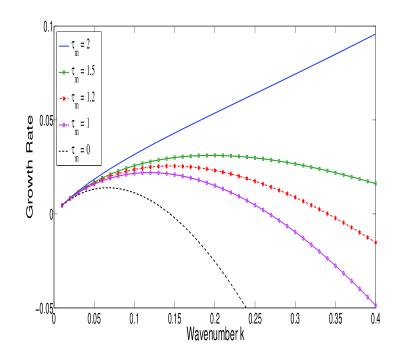
Figure 1: (Color online)Variation of growth rate with wave number is plotted for step shear profile with Reynolds Number $R=1$ and for different values of $\tau_{m}$ enlisted in legend. With increase of relaxation time $\tau_{m}$, growth rate also increases for each k.

Figure (1) shows a plot of growth rate vs. wave number for various values of $\tau_{m}$. For $\tau_{m}=0$, the dotted curve shows the result in a weakly coupled limit. This figure clearly indicates that increase of relaxation time enhances instability. Strong coupling between dust particles ($\Gamma$) increases relaxation time ($\tau_{m}$) Feng et al. (2010) and thus enhances the growth rate of KH instability.

III Eigenvalue Analysis

In the previous section, non-local analysis has shown that strong coupling between neighboring dust particles enhances the instability of parallel sheared dust flow. As a step profile is not a realistic profile, a $tanh$ type profile is considered which is widely treated in both experimental and simulation studies. The expression of such a profile is given by

$$v_{0}=\bar{v}_{0}\tanh(y/L),$$

where $L$ is typically the velocity shear inhomogeneity length and $\bar{v}_{0}$ is the magnitude of velocity far away from shear region. Hence the velocity smoothly varies from $-\bar{v}_{0}$ to the value $\bar{v}_{0}$ in the width of shear region $2L$. We have done matrix eigenvalue analysis of the differential equation (9) for the above mentioned profile using standard eigenvalue subroutine (eig)in MATLAB after properly discretization of the said equation with standard finite difference discretization scheme. Following central difference scheme is used for the purpose of discretization.

$$\frac{{\textstyle d^{4}\/\phi}}{{\textstyle d\/y^{4}}}=\frac{\phi_{i+2}-4\phi_{i+1}+6\phi_{i}-4\phi_{i-1}+\phi_{i-2}}{\Delta^{4}}$$

$$\frac{{\textstyle d^{2}\/\phi}}{{\textstyle d\/y^{2}}}=\frac{\phi_{i+1}-2\phi_{i}+\phi_{i-1}}{\Delta^{2}}~{}~{}~{}~{}~{}~{}~{}~{}~{}~{}~{}~{}~{}~{}~{}~{}~{}~{}~{}$$

$$\frac{{\textstyle d\/\phi}}{{\textstyle d\/y}}=\frac{\phi_{i+1}-\phi_{i-1}}{2\Delta}~{}~{}~{}~{}~{}~{}~{}~{}~{}~{}~{}~{}~{}~{}~{}~{}~{}~{}~{}~{}~{}~{}~{}~{}~{}~{}$$

where $\Delta$ is the grid spacing. After a few algebraic steps, the linearized fourth order equation(9) reduces to polynomial eigenvalue problem in $\omega$as

$$\left[A_{0}-\omega A_{1}-\omega^{2}A_{2}\right]\phi=0,$$ (16)

where $A_{i}$’s are the matrix elements in above equation and $\omega=kc$ ($c$ is the phase velocity). The polynomial eigenvalue problem can be changed into general eigenvalue problem using the dummy variable $\chi=\omega\phi$. Hence, the new eigenvalue problem is

$$\left(\begin{array}[]{lr}A_{0}&Z\\ Z&I\\ \end{array}\right)\left(\begin{array}[]{c}\phi\\ \chi\\ \end{array}\right)=\omega\left(\begin{array}[]{lr}A_{1}&A_{2}\\ I&Z\\ \end{array}\right)\left(\begin{array}[]{c}\phi\\ \chi\\ \end{array}\right),$$ (17)

where $I$ is identity matrix and $Z$ is a null matrix. This trick simplifies original polynomial eigenvalue problem into a simple and well known matrix eigenvalue problem as

$$R\bar{\phi}=\omega S\bar{\phi}$$

where

$$R=\left(\begin{array}[]{lr}A_{0}&Z\\ Z&I\\ \end{array}\right);~{}~{}\\ S=\left(\begin{array}[]{lr}A_{1}&A_{2}\\ I&Z\\ \end{array}\right);~{}~{}\\ \bar{\phi}=\left(\begin{array}[]{c}\phi\\ \chi\\ \end{array}\right).$$

Now, we can use eig subroutine to solve the eigenvalue equation. We have calculated the imaginary part of eigenvalues $\omega$, the positive value of which indicates the growth rate of the KH mode. First we should validate our code with respect to existing results. In weakly coupled limit($\tau_{m}\ll 1$), equation(9) reduces to the well known Orr-Somerfeld equation which has been thoroughly studied in the last century.

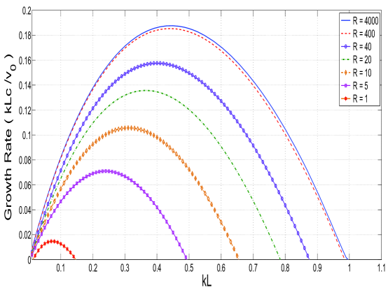
Figure 2: (Color online)Growth rate for different Reynolds Number(R) is plotted against wavenumber in weakly coupled limit ($\tau_{m}=0$). Growth rate($kc$) is calculated in unit of $v_{0}/L$ and wavenumber($k$) in unit of $1/L$. Different colors indicate different values of R. Viscous stabilization is clearly seen for small R and its large value proceeds towards inviscid limit $R\rightarrow\infty$.

In figure (2), we have plotted the growth rate against wave number for different values of Reynolds number $R$. These results agree with the results of Fig. 1. in Ref. Betchov and Szewczyk (1963). The code also shows that instability of $tanh$ velocity profile increases as viscosity decreases and for very large value of Reynolds number $R$, the result resemble to those obtained in the inviscid limit.

After this bench marking result, we investigate the growth rate of KH instability for different values of viscosity and relaxation time. The fact is that unstable mode has no real part i.e., it lies on the imaginary axis in the complex plane. In figure (3), eigenvalues in the complex plane have been plotted for $R=1,10$ and $\tau_{m}=1$ and the corresponding localized eigenfunctions are also shown. In figures (5)-(7), we have also shown growth rate vs. wave number curve for different values of $\tau_{m}$. As Reynolds number increases, growth rate for different $\tau_{m}$ values also increases.

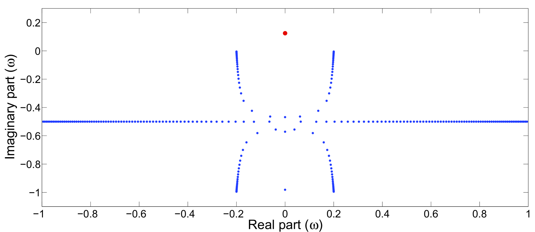
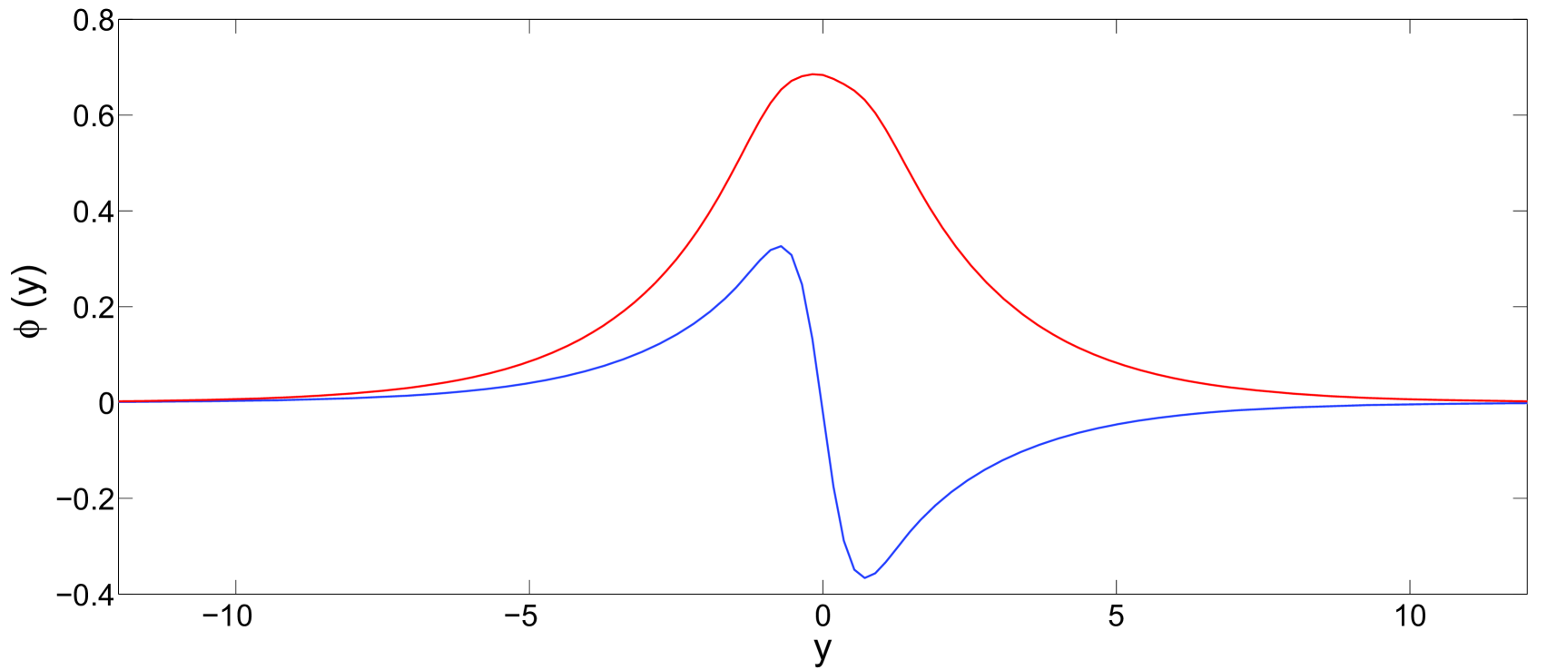
Figure 3: (Color online)Eigenvalues are shown in complex plane for $\tau_{m}=1$ and $R=10$ in the left graph. Red(big) dot represents the only unstable mode which is purely imaginary. Real(blue(lower) line) and imaginary(red(upper) line) parts of eigenfunction corresponding to unstable mode are plotted in the right graph.

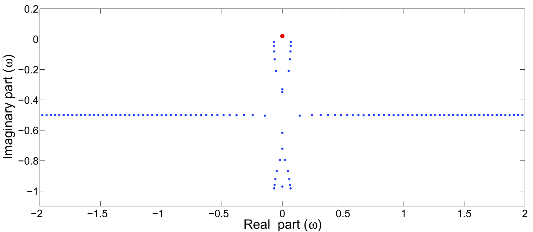
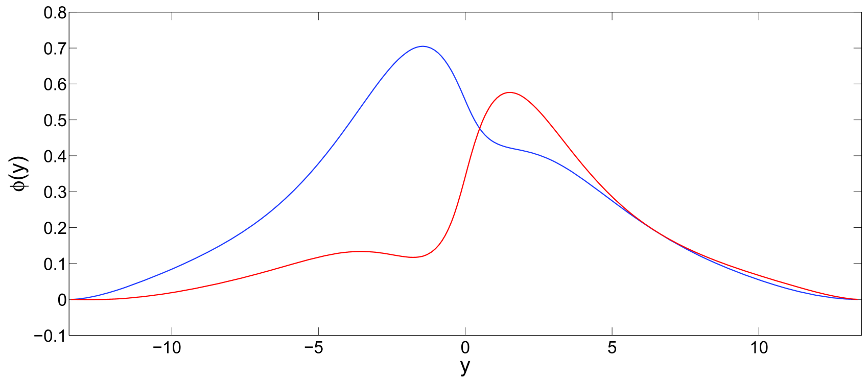
Figure 4: (Color online)Eigenvalues are shown in complex plane for $\tau_{m}=1$ and $R=1$ in the left graph. Red(big) dot represents the only unstable mode which is purely imaginary. Real(blue(upper) line) and imaginary(red(lower) line) parts of eigenfunction corresponding to unstable mode are shown in the right graph.

Reynolds number(R)	$\tau_{m}$	Max Growth rate	Max Growth rate
		with $\tau_{m}({\bf v}\cdot\nabla)$	without $\tau_{m}({\bf v}\cdot\nabla)$
	$0.0$	$0.01474$	$~{}~{}~{}~{}~{}~{}~{}~{}~{}0.01474$
	$1.0$	$0.02256$	$~{}~{}~{}~{}~{}~{}~{}~{}~{}0.01499$
	$2.0$	$0.07569$	$~{}~{}~{}~{}~{}~{}~{}~{}~{}0.01520$
$1$	$3.0$	$0.1069$	$~{}~{}~{}~{}~{}~{}~{}~{}~{}0.01575$
	$5.0$	$0.2267$	$~{}~{}~{}~{}~{}~{}~{}~{}~{}0.01621$
	$8.0$	$0.3197$	$~{}~{}~{}~{}~{}~{}~{}~{}~{}0.01690$
	$10.0$	$0.3545$	$~{}~{}~{}~{}~{}~{}~{}~{}~{}0.0179$

Table 1: Comparison of growth rates for Galilean invariant and non-invariant GH model

The Generalized Hydrodynamic model is becoming an inevitable tool to study the effect of strong coupling between dust particles on different waves and instabilities in a dusty plasma. In many cases, proper model was not taken into consideration. For the study of Kelvin-Helmholtz instability where equilibrium shear flow plays an important role, it is necessary to consider a proper Galilean invariant GH model. With the convective terms associated with relaxation time taken into account the growth rate of unstable mode is plotted against wave number in fig. (5) for $R=1$ in both cases of including or excluding the term $\tau_{m}\left({\bf v}\cdot\nabla\right)$. These two figures clearly indicate that the proper Galilean invariant form of the GH model makes a drastic change in growth rate using $tanh$ type velocity profiles. A comparison of growth rates is given in tabular form for different $\tau_{m}$ values. It is also observed that the limiting value of k beyond which instability vanishes also changes for different values of relaxation time $\tau_{m}$.

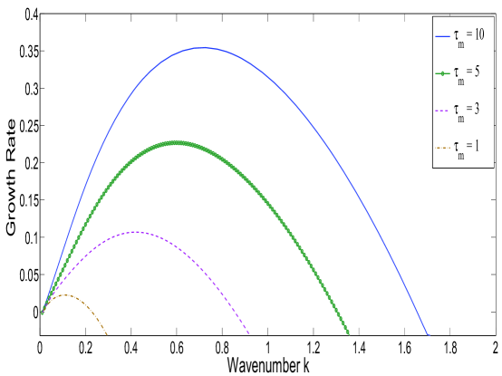
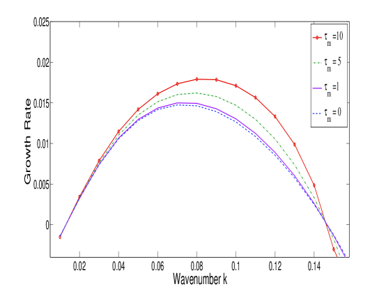
Figure 5: (Color online)Growth rate vs. wavenumber curves are shown for different values $\tau_{m}$ for two different cases – left one with taking $\tau_{m}\left({\bf v}\cdot\nabla\right)$ term in GH model and right one without that term. $R=1$.

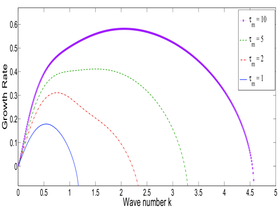
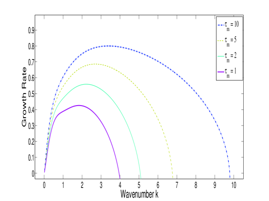
Figure 6: (Color online)For $R=5$ (left panel) and $R=10$ (right panel) and different values of $\tau_{m}$, variation of Growth rate with k is shown.

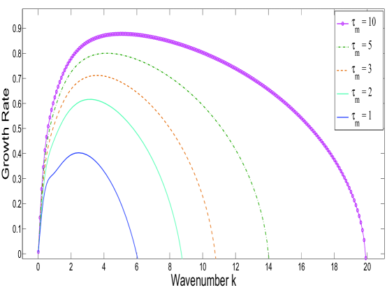
Figure 7: (Color online)In left figure, growth rate vs. $k$ is plotted for $R=40$ and different $\tau_{m}$. Right figure shows growth rate variation with $k$ for $\tau_{m}=5$ but different Reynolds numbers.

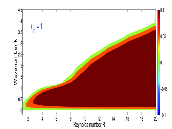
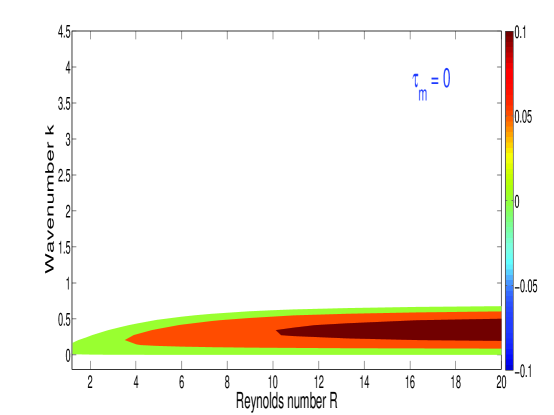
Figure 8: (Color online)Contour plot of growth rate of KH instability in 2D plane of $k$ and $R$ is shown for weakly coupled limit $\tau_{m}=0$ in the right panel. Colorbar indicates the values of growth rate in different color region. In the left panel, the same contour is plotted for relaxation time $\tau_{m}=1$ which shows rapid increase of unstable region in presence of strong coupling.

In figure (8) & (9), contour plot is being shown in 2D plane of Reynolds number and wavenumber which clearly shows that unstable region in this parameter space increases with effect of elasticity.

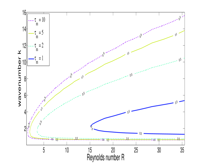
Figure 9: (Color online)Contour plot in 2D plane of $k$ and $R$ shows that unstable region increases with increase of relaxation time. Here, curves of growth rate $0.5$ are plotted for different values of $\tau_{m}$ enlisted in legend.

IV Summary

We have studied Kelvin-Helmholtz instability of dust shear flow with effects of both viscosity and elasticity in strongly coupled dusty plasma. Viscosity being a dissipative effect, plays stabilizing role. However, elasticity which has energy storing property changes the growth rate of KH instability. The growth rate of Kelvin-Helmholtz instability are estimated using proper Galilean invariant form of the GH equation. The stability characteristics of a small wave-number perturbation are studied analytically by using a discontinuous velocity profile. The combined effect of visco-elastic relaxation time $\tau_{m}$ and the additional convective term that assures Galilean invariance leads to a modification of the jump conditions and the eigenvalue equation. The results indicate a substantial enhancement of the growth rate and the range of unstable wave numbers over a wide variation of Reynolds number. The results are further confirmed through a numerical study by choosing a more realistic continuous velocity profile. In the limit $\tau_{m}\rightarrow 0$, the numerical results reproduce the standard Navier-Stoke’s results. In the absence of the convective term, bunching of the curves is observed with the growth rate vanishing at a particular wave number that is independent of $\tau_{m}$. However, the inclusion of the convective term in the GH operator causes a wide dispersion for the growth rate curves obtained for different values of $\tau_{m}$ at large values of wave numbers in contrast to the results obtained without the convective term. The results indicate that shear flows are unstable over a large range of wave numbers making their further study useful in context of strongly coupled dusty plasma.

References

• Shukla and Stenflo (2003) P. K. Shukla and L. Stenflo, Phys. Letters A 315, 244 (2003).
• Morfill et al. (1999) G. E. Morfill, H. M. Thomas, U. Konopka, and M. Zuzic, Phys. Plasmas 6, 1769 (1999).
• Pieper and Goree (1996) J. Pieper and J. Goree, Phys. Rev. Lett. 77, 3137 (1996).
• Melzer et al. (1997) A. Melzer, A. Homann, and A. Piel, Phys. Rev. E 53, 2757 (1997).
• Nosenko and Goree (2004) V. Nosenko and J. Goree, Phys. Rev. Lett. 93, 155004 (2004).
• Ikeji (1986) H. Ikeji, Phys. Fluids 29, 1764 (1986).
• Ichimaru (1982) S. Ichimaru, Rev. Mod. Phys. 54, 1017 (1982).
• Sorasio et al. (2003) G. Sorasio, P. K. Shukla, and D. P. Resendes, New. J. Phys.. 5, 81 (2003).
• Thomas and Morfill (1996) H. Thomas and G. Morfill, Nature (London) 379, 806 (1996).
• Kaw and Sen (1998) P. Kaw and A. Sen, Phys. Plasmas 5, 3552 (1998).
• Pramanik et al. (2002) J. Pramanik, G. Prasad, A. Sen, and P. Kaw, Phys. Rev. Lett. 88, 17500 (2002).
• Banerjee et al. (2010) D. Banerjee, M. S. Janaki, N. Chakrabarti, and M. Chaudhuri, New J. Phys. 12, 123031 (2010).
• D’Angelo and Song (1990) N. D’Angelo and B. Song, Planet. Space Sci. 38, 1577 (1990).
• Ashwin and Ganesh (2010) J. Ashwin and R. Ganesh, Phys. Rev. Lett. 104, 21503 (2010).
• Frenkel (1946) Y. Frenkel, Kinetic Theory of Liquids (Clarendon, Oxford, 1946).
• Ghosh et al. (2011) S. Ghosh, M. R. Gupta, N. Chakrabarti, and M. Chadhuri, Phys. Rev. E 83, 066406 (2011).
• Panton (1984) R. L. Panton, Incompressible Flow (John Wiley & Sons, New York, 1984).
• Drazin and Reid (1981) P. G. Drazin and W. H. Reid, Hydrodynamic Stabiity (Cambridge University Press, Cambridge, 1981).
• Drazin (1961) P. Drazin, J. Fluid Mech. 10, 571 (1961).
• Feng et al. (2010) Y. Feng, J. Goree, and B. Liu, Phys. Rev. E 82, 036403 (2010).
• Betchov and Szewczyk (1963) R. Betchov and A. Szewczyk, Phys. Fluids 6, 1391 (1963).