Wave packet dynamics and zitterbewegung of heavy holes in a quantizing magnetic field

Abstract

In this work we study wave packet dynamics and $zitterbewegung$, an oscillatory quantum motion, of heavy holes in III-V semiconductor quantum wells in presence of a quantizing magnetic field. It is revealed that a Gaussian wave-packet describing a heavy hole diffuses asymmetrically along the circular orbit while performing cyclotron motion. The wave packet splits into two peaks with unequal amplitudes after a certain time depending on spin-orbit coupling constant. This unequal splitting of the wave packet is attributed to the cubic Rashba interaction for heavy holes. The difference in the peak amplitudes disappears with time. At a certain time the two peaks diffuse almost along the entire cyclotron orbit. Then tail and head of the diffused wave packet interfere and as a result a completely randomized pattern of the wave packet is observed. The diffusion rate of the wave packet increases with increase of the spin-orbit interaction strength. Also strong spin-orbit coupling expedite the splitting and the randomization of the wave packet. We also study the $zitterbewegung$ in various physical observables such as position, charge current and spin angular momentum of the heavy hole. The $zitterbewegung$ oscillations are very much sensitive to the initial wave vector of the Gaussian wave packet and the strength of the Rashba spin-orbit coupling.

I Introduction

Spin dependent transport phenomena in low-dimensional semiconductor structures have been of a lot of interest to the scientific community in recent years due to the potential applications in the highly emerging field of spintronics.winkler ; fabian ; zutic ; cahay Intense research in this field was initiated after the proposal of spin field effect transistor by Datta and Das datta . The principal aim of this field is to produce pure spin current and its manipulation on semiconductor nanostructure devices. One important tool for generating pure spin current is the well known spin Hall effect (SHE). hirsch ; zhang ; murakami ; sinova ; hankie ; kato ; sheng ; wund In SHE spin-orbit interaction (SOI) leads to a generation of spin current from an external electric voltage. For the happening of SHE, the charge carriers are either electrons in the conduction band or holes in the valence band in a III-V semiconductor such as GaAs. Many $p$-doped semiconductors such as GaAs, InSb, Si etc show four-fold degeneracy in their valence band around the $\Gamma$ point. This kind of systems is described by $4\times 4$ LuttingerLutt Hamiltonian. The Luttinger Hamiltonian leads to two two-fold degenerate energy branches having different effective masses. These two dispersion branches are known as the heavy-hole (HH) and light-hole (LH) bands which are described by $j_{z}=\pm 3/2$ and $j_{z}=\pm 1/2$, respectively. For spin-orbit coupled two-dimensional hole system (2DHS) in a narrow quantum well, the $4\times 4$ Luttinger Hamiltonian can be projected onto $|3/2,\pm 3/2\rangle$ HH states giving rise to an effective $2\times 2$ Rashba Hamiltoniansczhang ; rwink ; loss provided that the hole density is sufficiently low. In 2DHS the Rashba SOI is tri-linear in momentum.

In recent years an oscillatory quantum motion, called $zitterbewegung$ (ZB), has become a central point of research interest in various low-dimensional semiconducting systems. The length and time scales corresponding to this trembling motion in vacuum are of the order of the Compton wavelength $\lambda_{c}=\hbar/m_{0}c\sim 10^{-4}$ nm and $\hbar/(2m_{0}c^{2})\sim 10^{-22}$ s, respectively. Due to this ultra small length and time scale, it has not been possible to make an experimental verification of ZB phenomenon in vacuum so far. However an intense interest was initiated around 2005 by Zawadzkizawad1 who has drawn an analogy between the Dirac equation of a free Dirac electron and the ${\bf k}\cdot{\bf p}$ theory of the band structure of a narrow gap semiconductor. He was able to find out a new length scale $\lambda_{Z}\approx 7$ nm which is much larger than $\lambda_{c}$. Later, the problem of ZB of electrons and holes in III-V semiconductor quantum wells in the presence of spin-orbit interaction was studied by Schliemannschliem1 ; schliem2 et. al. These pioneering works initiated tremendous motivation for theoretical studies in search of ZB in various condensed matter systems such as crystalline solid,tmrush graphene,zawad2 ; rusin ; demi1 ; yang ; zawadzr ; jung1 ; jung2 ; rakhi ; costa carbon nanotubes,zawad2 ; zawad3 ; zawad5 Luttinger liquid,demi2 superconductor,cserti1 ultra-cold atom,vaishnav ; song topological insulators chang1 ; chang2 etc. It was also reported that the origin of the minimal conductivity kats in graphene can be explained in the light of the peculiar phenomenon ZB. Recently, a general theory for ZB has been developed by David and Cserti.cserti2 Winklerwinkler2 et. al. considered a number of effective Hamiltonians representing different systems and studied various consequences of ZB oscillations. The effect of an in-plane magnetic field on the ZB oscillations in a Rashba-Dresselhaus system has been studied.ghosh Very recently, a complex quantum motion known as “super zitterbewegung” in graphene has been studiedrushin5 theoretically using time-dependent two-band Hamiltonian in the framework of rotating wave approximation.

Although the ZB phenomenon in vacuum is not yet observed experimentally, however an optical and acoustic analog of relativistic ZB have been observed experimentally in optical super-latticefelix and in a two-dimensional sonic crystalliu , respectively. Also simulationgerrit of Dirac particles has been performed recently using trapped ions and laser excitations. Most recently, the ZB in ⁸⁷Rb Bose-Einstein condensate is observed experimentally spielman ; Engels using direct imaging technique.

In this work we consider the long standing problem of ZB of heavy holes with cubic Rashba interaction in a III-V semiconductor quantum well subjected to a perpendicular magnetic field. We study time-evolution of a heavy hole represented by the Gaussian wave packet. We visualize and discuss how the hole wave packet evolves with time around the cyclotron orbit. It is shown that as time goes on, the initial wave packet starts to diffuse asymmetrically along the cyclotron orbit while executing cyclotron motion. At a later time, depending on the spin-orbit strength, the wave packet splits into two peaks with unequal amplitudes. After many more cycles, the wave packet diffuses entirely along the cyclotron orbit. Then interference occurs between tail and head of the diffused wave packet, which randomizes the wave packet along the entire cyclotron orbit. The ZB of heavy holes in various physical quantities, such as position, charge current and spin angular momentum, are studied analytically as well as numerically. It is revealed that the ZB in these observables are very much dependent on the initial wave vector of the Gaussian wave packet and the Rashba spin-orbit interaction.

This paper is organized in the following way. In section II we present all relevant theoretical details such as the Hamiltonian, Landau levels, its corresponding eigenfunction and time-evolution of initial hole wave packet using Green’s function approach as well as average values of various physical observables. Numerical results and discussion are given in section III. We summarize our findings in section IV. We present detailed calculations in Appendix A.

II Theoretical Calculations

II.1 Hamiltonian

The dynamics of holes in the $\Gamma_{8}$ valence band of III-V semiconductors with zinc-blende structure like GaAs are well described within the framework of the Luttinger model (LM). In the spherical approximationspheric of LM, the topmost valence band is four fold degenerate at the $\Gamma$ point with HH and LH bands corresponding to total spin $J=3/2$. Strong quantum confinement in the semiconductor heterostructure along the growth direction removes the $\Gamma$ point degeneracy between the HH and LH bands. At very low temperature and low density only the HH subbands are assumed to be occupied. Now, it is possible to obtain a $k$-cubic Rashba Hamiltonian from the Luttinger Hamiltonian by projecting the latter onto the HH states.

It is well knownrwink ; sczhang that the Rashba spin-splitting for HH and LH bands are proportional to $k^{3}$ and $k$, respectively. The linear spin-splitting for LHs is similar to that for electrons.rashba Our present study mainly deals with only HHs and hence linear spin-splitting for electrons and LHs is completely ignored.

In presence of a perpendicular magnetic field the single particle Hamiltonian tianx ; zarea of a 2DHS with Rashba SOI (RSOI) can be written as

$$H=\frac{{\bf\Pi}^{2}}{2m^{\ast}}+\frac{i\alpha}{2\hbar^{3}}\Big{(}\Pi_{-}^{3}\sigma_{+}-\Pi_{+}^{3}\sigma_{-}\Big{)}-g_{s}\mu_{B}{\bf J}\cdot{\bf B},$$ (1)

where ${\bf\Pi}={\bf p}-e{\bf A}$ with ${\bf p}$ is the canonical momentum operator, ${\bf A}$ is the vector potential corresponding to the external magnetic field ${\bf B}$, ${\bf J}=(3/2){\bm{\sigma}}$, $m^{\ast}$ is the effective mass of the heavy hole, $\alpha$ is the Rashba coupling coefficient and $\sigma_{i}$ ’s are the Pauli matrices. Also, $\Pi_{\pm}=\Pi_{x}\pm i\Pi_{y}$, $\sigma_{\pm}=\sigma_{x}\pm i\sigma_{y}$ and $g_{s}$ is the effective Lande g-factor. One important point to be mentioned here that the Pauli matrices represent an effective pseudo-spin with spin projection $\pm 3/2$ along the growth direction of the quantum well.

For convenience, we assume ${\bf B}=-B\hat{z}$ and the corresponding vector potential in the Landau gauge as ${\bf A}=(By,0,0)$. The Hamiltonian $H$ in Eq. (1) commutes with $p_{x}$. Hence the wave vector $k_{x}$ is a good quantum number. In matrix form the Hamiltonian takes the following form:

$$H=\hbar\omega_{c}\begin{pmatrix}h_{0}+\chi&-i\tilde{\alpha}h_{-}^{3}\\ i\tilde{\alpha}h_{+}^{3}&h_{0}-\chi\\ \end{pmatrix},$$ (2)

where $h_{0}=(-\partial^{2}/\partial\eta^{2}+\eta^{2})/2$ is the oscillator Hamiltonian and $h_{\pm}=(\eta\mp\partial/\partial\eta)/\sqrt{2}$ is the creation (annihilation) operator. Here, $\eta=(y-y_{c})/l_{0}$ with $y_{c}=l_{0}^{2}k_{x}$ and $l_{0}=\sqrt{\hbar/(eB)}$ is the magnetic length. Also, $\omega_{c}=eB/m^{\ast}$ is the cyclotron frequency, the dimensionless Rashba parameter $\tilde{\alpha}=2\sqrt{2}\alpha/(l_{0}^{3}\hbar\omega_{c})$ and $\chi=3g_{s}m^{*}/(4m_{e})$. The operations of $h_{0}$ and $h_{\pm}$ on the oscillator wave functions $\phi_{n}(\eta)=\sqrt{1/(2^{n}n!\sqrt{\pi}l_{0})}e^{-\eta^{2}/2}H_{n}(\eta)$ are $h_{0}\phi_{n}(\eta)=(n+1/2)\phi_{n}(\eta)$, $h_{+}\phi_{n}(\eta)=\sqrt{n+1}\phi_{n+1}(\eta)$ and $h_{-}\phi_{n}(\eta)=\sqrt{n}\phi_{n-1}(\eta)$.

For $n\geq 3$ the energy eigenvaluestianx are given by

$$\epsilon_{n}^{\lambda}=\hbar\omega_{c}\Big{[}(n-1)+\lambda\sqrt{E_{0}^{2}+\tilde{\alpha}^{2}A_{n}}\Big{]},$$ (3)

where $\lambda=\pm$ represents two spin-split energy branches, $E_{0}=\chi-3/2$ and $A_{n}=n(n-1)(n-2)$. The eigenfunctions corresponding to the eigenvalues given in Eq. (3) are

$$\psi_{\xi}^{\lambda}({x,y})=\frac{e^{ik_{x}x}}{\sqrt{2\pi}}\left(\begin{array}[]{c}i\cos\theta_{n}^{\lambda}\phi_{n-3}(y-y_{c})\\ \sin\theta_{n}^{\lambda}\phi_{n}(y-y_{c})\\ \end{array}\right).$$ (6)

Here, $\xi:\{n,k_{x}\}$ is a set of two quantum numbers, $\tan\theta_{n}^{\lambda}=\tilde{\alpha}\sqrt{A_{n}}/B_{n}^{\lambda}$ with $B_{n}^{\lambda}=n+1/2-\chi-\epsilon_{n}^{\lambda}/(\hbar\omega_{c})$.

For $n<3$, the energy levels are $\epsilon_{n}^{+}=\hbar\omega_{c}(n+1/2-\chi)$ and the corresponding eigenfunctions are

$$\psi_{\xi}^{+}({x,y})=\frac{e^{ik_{x}x}}{\sqrt{2\pi}}\left(\begin{array}[]{c}0\\ \phi_{n}(y-y_{c})\\ \end{array}\right).$$ (9)

II.2 Propagator construction and time-evolution of initial wave packet

In order to describe the time-evolution of an initial Gaussian wave packet it is necessary to construct an appropriate propagator. For this purpose we follow the well known Green’s function technique as described in Ref. [demi, ]. In matrix form, the propagator or the Green’s function can be written as

$$G({\bf r},{\bf r^{\prime}},t)=\begin{pmatrix}G_{11}({\bf r},{\bf r^{\prime}},t)&G_{12}({\bf r},{\bf r^{\prime}},t)\\ G_{21}({\bf r},{\bf r^{\prime}},t)&G_{22}({\bf r},{\bf r^{\prime}},t)\\ \end{pmatrix}.$$ (10)

The matrix elements of Eq. (10) are defined as

$$G_{ij}({\bf r},{\bf r^{\prime}},t)=\sum_{\lambda=\pm}\int dk_{x}\sum_{n=0}^{\infty}\psi_{\xi,i}^{\lambda}({\bf r},t)\psi_{\xi,j}^{\lambda^{\ast}}({\bf r}^{\prime},0).$$ (11)

Here, the indices $i,j=1,2$ represent the upper/lower components of the wave functions. The hole wave function at a later time $t$ is given by $\psi_{\xi}^{\lambda}({\bf r},t)=\psi_{\xi}^{\lambda}({\bf r},0)e^{-i\epsilon_{n}^{\lambda}t/\hbar}$, where $\psi_{\xi}^{\lambda}({\bf r},0)$ ’s are given by Eqs. (6) and (9).

In presence of the perpendicular magnetic field, we represent an initial state of the hole by a Gaussian wave packet with the initial spin polarization along the $z$ axis as given by

$$\Psi({\bf r},0)=\frac{1}{\sqrt{\pi}l_{0}}\exp\Big{(}-\frac{r^{2}}{2l_{0}^{2}}+i\frac{p_{0x}x}{\hbar}\Big{)}\left(\begin{array}[]{c}1\\ 0\\ \end{array}\right),$$ (14)

where $p_{0x}=\hbar k_{0x}$ is the initial momentum of the wave packet along $x$ direction. Note that the initial state coincides with the coherent state of a charge particle in a magnetic field. We have taken such wave function because the dynamics of coherent states in a magnetic field resembles the dynamics of a classical particle.

The choice of the two component spinor considered in Eq. (14) is completely arbitrary. It can have both nonzero components as discussed in Refs. [rusin, ; demi1, ; zawad5, ].

In general the time-evolution of the initial wave packet can be obtained with the help of the Green’s function as given by

$$\Psi({\bf r},t)=\int d{\bf r}^{\prime}G({\bf r},{\bf r}^{\prime},t)\Psi({\bf r}^{\prime},0).$$ (15)

Using Eq. (10), (14) and (15) one can obtain

$$\left(\begin{array}[]{c}\Psi_{1}({\bf r},t)\\ \Psi_{2}({\bf r},t)\\ \end{array}\right) = \frac{1}{\sqrt{\pi}l_{0}}\int d{\bf r}^{\prime}\exp\Big{(}-\frac{{r^{\prime}}^{2}}{2l_{0}^{2}}+i\frac{p_{0x}x^{\prime}}{\hbar}\Big{)}$$ (18)

$$\times \left(\begin{array}[]{c}G_{11}({\bf r},{\bf r}^{\prime},t)\\ G_{21}({\bf r},{\bf r}^{\prime},t)\\ \end{array}\right).$$ (21)

It is straightforward to calculate the required matrix elements of the Green’s function and these are given by

$$G_{11}({\bf r},{\bf r}^{\prime},t) = \frac{1}{2\pi}\int_{-\infty}^{\infty}dk_{x}e^{ik_{x}(x-x^{\prime})}\sum_{n=0}^{\infty}\Gamma_{n+3}(t)$$ (22)

$$\times \phi_{n}(y-y_{c})\phi_{n}(y^{\prime}-y_{c})$$

and

$$G_{21}({\bf r},{\bf r}^{\prime},t) = \frac{1}{2\pi}\int_{-\infty}^{\infty}dk_{x}e^{ik_{x}(x-x^{\prime})}\sum_{n=0}^{\infty}\Delta_{n+3}(t)$$ (23)

$$\times \phi_{n+3}(y-y_{c})\phi_{n}(y^{\prime}-y_{c}),$$

where $\Gamma_{n}(t)=e^{-i(n-1)\omega_{c}t}[\cos(\delta_{n}t)-i\xi_{n}\sin(\delta_{n}t)]$ and $\Delta_{n}(t)=e^{-i(n-1)\omega_{c}t}\zeta_{n}\sin(\delta_{n}t)$ with $\delta_{n}=\omega_{c}\sqrt{E_{0}^{2}+\tilde{\alpha}^{2}A_{n}}$, $\xi_{n}=E_{0}/\sqrt{E_{0}^{2}+\tilde{\alpha}^{2}A_{n}}$ and $\zeta_{n}=\tilde{\alpha}\sqrt{A_{n}}\xi_{n}/E_{0}$. Note that $\Gamma_{n}(t=0)=1$ and $\Delta_{n}(t=0)=0$. It is easy to verify an interesting result that $|\Gamma_{n}(t)|^{2}+|\Delta_{n}(t)|^{2}=1$.

The components of the wave packet at a later time $t$ are given by

$$\Psi_{1}({\bf r},t) = \frac{1}{\sqrt{2}\pi l_{0}}\sum_{n=0}^{\infty}(-1)^{n}\frac{\Gamma_{n+3}(t)}{2^{n}n!}$$ (24)

$$\times \int_{-\infty}^{\infty}due^{\Lambda(x,y,u)}u^{n}H_{n}(y/l_{0}-u)$$

and

$$\Psi_{2}({\bf r},t) = \frac{1}{4\pi l_{0}}\sum_{n=0}^{\infty}(-1)^{n}\frac{\Delta_{n+3}(t)}{2^{n}n!\sqrt{A_{n+3}}}$$ (25)

$$\times \int_{-\infty}^{\infty}due^{\Lambda(x,y,u)}u^{n}H_{n+3}(y/l_{0}-u),$$

where $u=k_{x}l_{0}$ and $\Lambda(x,y,u)=iux/l_{0}-(a-u)^{2}/2-u^{2}/4-(y/l_{0}-u)^{2}/2$ with $a=k_{0x}l_{0}$.

II.3 Zitterbewegung in position and velocity

In this section we find the average values of the position and velocity operators. The time-dependent average value of the position operator is given by

$$\left(\begin{array}[]{c}\langle x\rangle\\ \langle y\rangle\\ \end{array}\right)=\sum_{i=1,2}\int d{\bf r}\Psi_{i}^{\ast}({\bf r},t)\left(\begin{array}[]{c}x\\ y\\ \end{array}\right)\Psi_{i}({\bf r},t).$$ (30)

It is straightforward to calculate the average values of $x$ and $y$ using Eqs. (24) and (25). Detailed calculations are given in Appendix A. The average values of $x$ and $y$ are given by

$$\langle x(t)\rangle = L\sum_{n=0}^{\infty}\frac{i(-1)^{n+1}}{n!(12)^{n}}\Big{\{}\mathrm{Im}\,(\Gamma_{n+4}^{\ast}\Gamma_{n+3})+\sqrt{\frac{n+4}{n+1}}$$ (31)

$$\times \mathrm{Im}\,(\Delta_{n+4}^{\ast}\Delta_{n+3})\Big{\}}H_{2n+1}(i\sqrt{2/3}a)$$

and

$$\langle y(t)\rangle = L\sum_{n=0}^{\infty}\frac{i(-1)^{n}}{n!(12)^{n}}\Big{\{}\mathrm{Re}\,(\Gamma_{n+4}^{\ast}\Gamma_{n+3})+\sqrt{\frac{n+4}{n+1}}$$ (32)

$$\times \mathrm{Re}\,(\Delta_{n+4}^{\ast}\Delta_{n+3})-1\Big{\}}H_{2n+1}(i\sqrt{2/3}a),$$

where $L=\frac{l_{0}}{3}\exp(-a^{2}/3)$.

The velocity operator is obtained from the commutation relation ${\bf v}=[{\bf r},H]/(i\hbar)$. The components of the velocity operator are given by

$$v_{x}=\frac{\Pi_{x}}{m^{\ast}}\sigma_{0}+\frac{3i\alpha}{2\hbar^{3}}(\sigma_{+}\Pi_{-}^{2}-\sigma_{-}\Pi_{+}^{2})$$ (33)

and

$$v_{y}=\frac{\Pi_{y}}{m^{\ast}}\sigma_{0}+\frac{3\alpha}{2\hbar^{3}}(\sigma_{+}\Pi_{-}^{2}+\sigma_{-}\Pi_{+}^{2}).$$ (34)

The average value of the velocity operator is given by

$$\langle v_{k}(t)\rangle=\int dxdy\left(\begin{array}[]{c}\Psi_{1}^{\ast}\ \Psi_{2}^{\ast}\end{array}\right){v_{k}}\left(\begin{array}[]{c}\Psi_{1}\\ \Psi_{2}\end{array}\right),$$ (38)

where the index $k$ represents the $x$ and $y$ components of the velocity. Using Eqs. (24), (25) and (38), after a lengthy but straightforward calculation, we finally obtain average values of the components of the velocity operator as

$$\langle v_{x}(t)\rangle = L\omega_{c}\sum_{n=0}^{\infty}\frac{i(-1)^{n+1}}{n!(12)^{n}}\Big{\{}\mathrm{Re}\,(\Gamma_{n+4}^{\ast}\Gamma_{n+3})+\sqrt{\frac{n+4}{n+1}}$$ (39)

$$\times \mathrm{Re}\,(\Delta_{n+4}^{\ast}\Delta_{n+3})+3\tilde{\alpha}\sqrt{\frac{(n+2)(n+3)}{n+1}}$$

$$\times \mathrm{Im}\,(\Gamma_{n+4}^{\ast}\Delta_{n+3})\Big{\}}H_{2n+1}(i\sqrt{2/3}a)$$

and

$$\langle v_{y}(t)\rangle = L\omega_{c}\sum_{n=0}^{\infty}\frac{i(-1)^{n+1}}{n!(12)^{n}}\Big{\{}\mathrm{Im}\,(\Gamma_{n+4}^{\ast}\Gamma_{n+3})+\sqrt{\frac{n+4}{n+1}}$$ (40)

$$\times \mathrm{Im}\,(\Delta_{n+4}^{\ast}\Delta_{n+3})-3\tilde{\alpha}\sqrt{\frac{(n+2)(n+3)}{n+1}}$$

$$\times \mathrm{Re}\,(\Gamma_{n+4}^{\ast}\Delta_{n+3})\Big{\}}H_{2n+1}(i\sqrt{2/3}a).$$

II.4 Zitterbewegung in spin angular momentum

Now we turn to concentrate on the ZB in the spin angular momentum of a heavy hole in the presence of a perpendicular magnetic field. In this sub-section we shall calculate the time-dependent average values of the components of the effective spin operator naka ; raichev ${\bf S}=\frac{3\hbar}{2}{\bm{\sigma}}$. The spatio-temporal profile of the hole spin density is defined as

$${\bf S}({\bf r},t)=\left(\begin{array}[]{c}\Psi_{1}^{\ast}\ \Psi_{2}^{\ast}\end{array}\right){\bf S}\left(\begin{array}[]{c}\Psi_{1}\\ \Psi_{2}\end{array}\right).$$ (44)

The time-dependent average value of the spin operator is given by

$$\langle{\bf S}(t)\rangle=\int{\bf S}({\bf r},t)dxdy.$$ (45)

The components of the average values of the spin operators are

$$\langle S_{x}(t)\rangle = \frac{\hbar}{\sqrt{2}}\exp(-a^{2}/3)\sum_{n=0}^{\infty}\frac{i(-1)^{n+1}}{n!(12)^{n+1}}$$ (46)

$$\times \frac{\mathrm{Re}\,(\Gamma_{n+6}^{\ast}\Delta_{n+3})}{\sqrt{A_{n+3}}}H_{2n+3}(i\sqrt{2/3}a),$$

$$\langle S_{y}(t)\rangle = \frac{\hbar}{\sqrt{2}}\exp(-a^{2}/3)\sum_{n=0}^{\infty}\frac{i(-1)^{n+1}}{n!(12)^{n+1}}$$ (47)

$$\times \frac{\mathrm{Im}\,(\Gamma_{n+6}^{\ast}\Delta_{n+3})}{\sqrt{A_{n+3}}}H_{2n+3}(i\sqrt{2/3}a)$$

and

$$\langle S_{z}(t)\rangle = \sqrt{\frac{3}{2}}\hbar\exp(-a^{2}/3)\sum_{n=0}^{\infty}\frac{(-1)^{n}}{n!(12)^{n}}$$ (48)

$$\times (|\Gamma_{n+3}|^{2}-|\Delta_{n+3}|^{2})H_{2n}(i\sqrt{2/3}a).$$

III Numerical results and discussions

In this section we shall visualize and discuss how the spatial distribution of probability density for the heavy holes changes with time. We shall also discuss the time dependencies of the expectation values of the position, current and spin operators and their various consequences. For numerical calculations, we adopt the material parameters appropriate for GaAs quantum wells. We took $m^{\ast}=0.45m_{0}$ with $m_{0}$ as the free electron mass, $k_{0}=10^{8}$ m^-1 and $B=1.5$ T. It was reported that the value of the effective Lande g-factor for heavy hole is highly anisotropicwinkg , we take its value $g^{\ast}=7.2$ for GaAs system.

The magnitude of Rashba strength ($\alpha$) depends explicitly on the external parametersrwink like electric field, detail of confinement and hence can be tuned experimentally. So in this study, we take various values of $\alpha$ in such a way that the corresponding length scale $l_{\alpha}=m^{\ast}\alpha/\hbar^{2}$ is of the order of few angstroms.

In Fig. (1) we show the time-evolution of the probability density $\rho({\bf r},t)=|\Psi_{1}({\bf r},t)|^{2}$ + $|\Psi_{2}({\bf r},t)|^{2}$ of the heavy hole. To do this we numerically evaluate the components of the wave packet $\Psi_{1}({\bf r},t)$ and $\Psi_{2}({\bf r},t)$ at a later time $t$ as described by Eqs. (24) and (25). The infinite series in Eqs. (24) and (25) converge approximately when $n=30$ for $k_{0x}=1.5k_{0}$. However the convergence of these infinite series also depends on the value of $k_{0x}$. For larger $k_{0x}$ larger $n$ is required. We have checked that $n=60$ is appropriate for the convergence when $k_{0x}=2.5k_{0}$. Figs. 1(a)-1(i) are plotted for $t=0,2t_{c},4t_{c},5t_{c},6t_{c},7t_{c},8t_{c},9t_{c}$ and $10t_{c}$, respectively. Initially the wave packet is situated at the origin. We know that in a perpendicular magnetic field a charge particle (without SOI) moves in a cyclotron orbit with time period $t_{c}=2\pi/\omega_{c}$. The radius of this circular orbit is $R_{c}=k_{0x}l_{0}^{2}$. The presence of SOI modifies $t_{c}$ and $R_{c}$ marginally. In presence of the RSOI the hole wave packet starts to diffuse asymmetrically around the cyclotron orbit while making circular motion as time goes on. The diffused wave packet is making circular motion with time period $\approx t_{c}$ and radius $\approx R_{c}$. At $t=4t_{c}$ [Fig 1(c)] the hole wave packet splits into two unequal peaks which are rotating with different velocities along the cyclotron orbit. The difference in the peak amplitudes nearly vanishes around $t=7t_{c}$ [Fig. 1(f)]. At the same time, the wave packet diffuses almost along the entire cyclotron orbit. Now the interference effect begins to occur between the tail and head of the diffused wave packet and as a result a completely randomized pattern of hole wave packet is observed after some more cycles as shown in Fig. 1(i). Recalling the case of two-dimensional electron system (2DES) with linear RSOI in a perpendicular magnetic field where this kind of splitting of wave packet occurs around $t\approx 45t_{c}$demi for $B=1$ T. But in the present case of 2DHS this splitting occurs at much lesser time than the 2DES case. Moreover, the wave-packet does not diffuse along the circular orbit in the case of 2DES with linear Rashba term. These features can be attributed to the cubic Rashba term in the 2DHS.

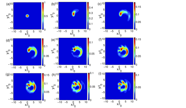
Figure 1: (Color online) Time-evolution of the hole wave packet in a magnetic field at (a) $t=0$, (b) $t=2t_{c}$, (c) $t=4t_{c}$, (d) $t=5t_{c}$, (e) $t=6t_{c}$, (f) $t=7t_{c}$, (g) $t=8t_{c}$, (h) $t=9t_{c}$, and (i) $t=10t_{c}$. In this case $\alpha$ is fixed in such a way that $l_{\alpha}=0.25$ nm. In each plot the color bar represents the dimensionless parameter $\pi l_{0}^{2}\rho({\bf r},t)$.

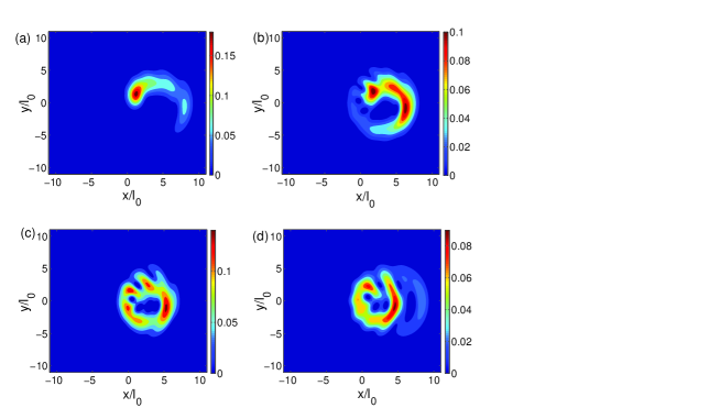
Figure 2: (Color online) Time-evolution of the hole wave packet in a magnetic field at $t=4t_{c}$ for different values of $l_{\alpha}=m^{\ast}\alpha/\hbar^{2}$ namely (a) $l_{\alpha}=0.25$ nm, (b) $l_{\alpha}=0.35$ nm, (c) $l_{\alpha}=0.45$ nm, and (d) $l_{\alpha}=0.55$ nm. In this case magnetic field and the initial wave vector are fixed to $B=1.5$ T and $k_{0x}=1.5k_{0}$. In each plot the color bar represents the dimensionless parameter $\pi l_{0}^{2}\rho({\bf r},t)$.

In Fig. 2 spatial distribution of probability density at time $t=4t_{c}$ is shown. Different panels are plotted for different values of $\alpha$ such that $l_{\alpha}=0.25$ nm, $0.35$ nm, $0.45$ nm, and $0.55$ nm. It is clear that as $\alpha$ increases the wave packet diffuses very fast and covers the entire cyclotron orbit. The diffusion rate of the wave packet increases with increase of the spin-orbit strength. Also strong $\alpha$ helps to expedite the splitting and the randomization of the hole wave packet.

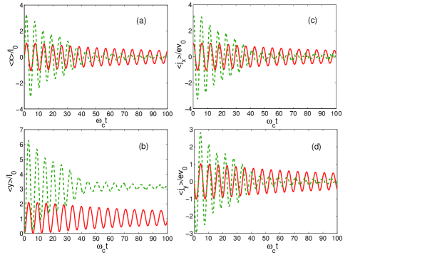
Figure 3: (Color online) Time dependence of position and current components: (a) $\langle x\rangle$, (b) $\langle y\rangle$, (c) $\langle j_{x}\rangle$, and (d) $\langle j_{y}\rangle$. Here in each panel solid and dashed lines correspond to $k_{0x}=0.5k_{0}$ and $1.5k_{0}$, respectively. Here $v_{0}$ is defined as $v_{0}=\hbar/(m^{\ast}l_{0})$.

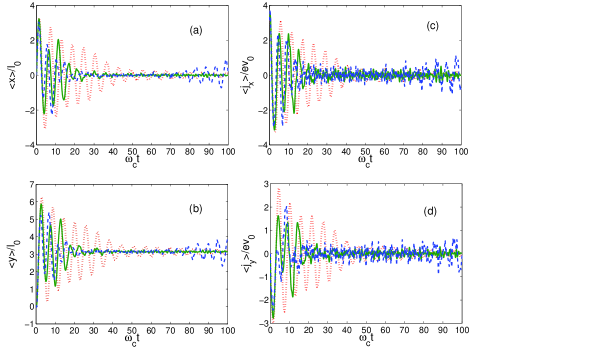
Figure 4: (Color online) Time dependence of position and current components: (a) $\langle x\rangle$, (b) $\langle y\rangle$, (c) $\langle j_{x}\rangle$, and (d) $\langle j_{y}\rangle$. Here in each panel dotted, solid and dashed lines correspond to $l_{\alpha}=0.25$, $0.5$, and $0.75$ nm, respectively. Here we define $v_{0}=\hbar/(m^{\ast}l_{0})$.

In Fig. 3 we plot the average values of the position and current operators in $x$ and $y$ directions as a function of time $t$ for a fixed value of magnetic field $B=1.5$ T and fixed $\alpha$ such that $l_{\alpha}=0.25$ nm. Here, we define the current operators as $j_{i}(t)=ev_{i}(t)$ with $i=x$, $y$. In this case we consider two different values of initial wave vector $k_{0x}=0.5k_{0}$ (solid line) and $k_{0x}=1.5k_{0}$ (dashed line). When $k_{0x}=0.5k_{0}$, oscillations appearing in $\langle x\rangle,\langle y\rangle,\langle j_{x}\rangle$ and $\langle j_{y}\rangle$ are persistent in time. But in the case of higher $k_{0x}$, the amplitude of ZB decreases at later time which shows some kind of localization of ZB oscillations. This is because higher Landau levels are involving for higher values of $k_{0x}$. Comparing Figs. 3(a) and 3(b) we mention that $\langle x\rangle$ is oscillating about zero for both values of $k_{0x}$ whereas $\langle y\rangle$ is oscillatory but always positive because Eq. (32) contains a constant term. There is also a definite phase difference between $\langle x\rangle$ and $\langle y\rangle$ and $\langle j_{x}\rangle$ and $\langle j_{y}\rangle$ as clearly shown in Fig. 3. Investigating all the graphs in Fig. (3) one can conclude that although initially there is no phase difference but an increment in $k_{0x}$ introduces a phase difference at later times.

Figure 4 describes the time dependence of position and current operators for a fixed magnetic field $B=1.5$ T and $k_{0x}=1.5k_{0}$. Different values of $\alpha$ such that $l_{\alpha}=0.25$ nm (dotted), $0.5$ nm (solid), and $0.75$ nm (dashed) have been considered. It can be seen from Fig. 4 that the amplitude of ZB oscillation decreases as $\alpha$ increases. One interesting point is to be mentioned here that at stronger $\alpha$ ($l_{\alpha}=0.75$ nm) the ZB oscillations start to reappear at large time.

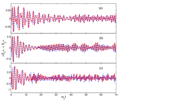
Figure 5: (Color online) Time dependence of the $x$ and $y$ components of the spin operator: (a) $k_{0x}=0.5k_{0}$, (b) $k_{0x}=1.5k_{0}$, and (c) $k_{0x}=2.5k_{0}$. Here in each panel solid and dashed lines represent $\langle S_{x}\rangle$ and $\langle S_{y}\rangle$, respectively which are plotted in units of $\hbar$.

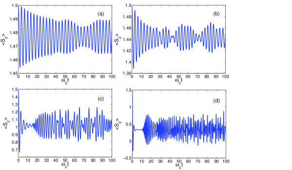
Figure 6: (Color online) Time dependence of the $z$ component of spin operator: (a) $k_{0x}=0$, (b) $k_{0x}=0.5k_{0}$, (c) $k_{0x}=1.5k_{0}$, and (d) $k_{0x}=2.5k_{0}$. Here in each panel $\langle S_{z}\rangle$ is plotted in units of $\hbar$.

The time-dependent average values of the spin components are shown in Fig. 5 and 6. We consider various cases corresponding to the different values of the initial wave vector, namely $k_{0x}=0$, $0.5k_{0}$, $1.5k_{0}$ and $2.5k_{0}$ as mentioned in both figures. Figure 5 describes the variations of $\langle S_{x}\rangle$ and $\langle S_{y}\rangle$ with time $t$ for different values of $k_{0x}$. It can be seen that $\langle S_{x}\rangle$ and $\langle S_{y}\rangle$ maintains same oscillatory pattern apart from a definite phase difference. An increase in $k_{0x}$ results a change in the oscillatory pattern significantly. The amplitude of the ZB oscillations, appearing in $\langle S_{x}\rangle$ and $\langle S_{y}\rangle$ increases as $k_{0x}$ increases. We have shown the time dependence of $\langle S_{z}\rangle$ in Fig. 6. It should be noted that $\langle S_{z}\rangle$ does not vanish when there is no initial momentum i.e. $k_{0x}=0$. This fact can be confirmed from Eq. (48) which contains a non-zero term $H_{2n}(0)$. As $k_{0x}$ increases the oscillatory pattern of $\langle S_{z}\rangle$ changes abruptly. When $k_{0x}=0.5k_{0}$ a beating-like pattern appears in the oscillations of $\langle S_{z}\rangle$. From Fig. 6(b), (c), (d) it can be seen that the number of oscillations before the first beating node decreases drastically as $k_{0x}$ increases. This complicated oscillatory pattern can be attributed to the fact that the infinite series in Eqs. (46-48) converges for higher values of $n$ as $k_{0x}$ increases. As a result more and more frequencies appear in the oscillations because of the involvement of higher Landau levels. Comparing Fig. 5 and 6 at $t=0$ $\langle S_{x}\rangle=0=\langle S_{y}\rangle$ where as $\langle S_{z}\rangle=3\hbar/2$ and this is consistent with the fact that the initial wave packet is polarized along the $z$-direction. The jittery motion in $S_{z}$ induces jittery motion in $S_{x}$ and $S_{y}$.

IV Summary

In summary, we have studied wave packet propagation and $zitterbewegung$ of a heavy hole in III-V semiconductor quantum wells. We have visualized and discussed various consequences of the time-evolution of the hole wave packet along the cyclotron orbit. The hole wave packet diffuses asymmetrically along the circular orbit while making cyclotron motion. It is shown that the hole wave packet splits into two peaks with unequal amplitudes at certain time which depends on the spin-orbit interaction strength. The two peaks rotate with different frequencies. The amplitude of the two peaks become nearly equal as time goes on. After many cycles, tail and head of the diffused wave packet interfere with each other and produces a complete randomized pattern. The diffusion rate of the wave packet increases with increase of the spin-orbit interaction strength. Also strong spin-orbit coupling expedite the splitting and the randomization of the wave packet. Our results for the hole is compared with an electron in a linear Rashba system in presence of the magnetic field. We have also studied ZB phenomenon in position, current and spin angular momentum of the heavy hole. The $zitterbewegung$ oscillations are very much sensitive to the initial momentum of the wave packet and the Rashba spin-orbit coupling constant.

Appendix A Expectation values position and velocity operators

In this appendix we shall present detailed derivation of the average values of various physical observables like position and velocity operators.

The calculation of the average value of the $y$ component of the position operator is easier than that of the $x$ component. Let us first calculate average value of the $x$ component. Equation (30) can be written as $\langle x(t)\rangle=\langle x_{1}(t)\rangle+\langle x_{2}(t)\rangle$, where $\langle x_{i}(t)\rangle=\int dxdy\Psi_{i}^{\ast}({\bf r},t)x\Psi_{i}({\bf r},t)$. The explicit form of $\langle x_{1}(t)\rangle$ is

$$\langle x_{1}(t)\rangle = \frac{1}{2\pi^{2}l_{0}^{2}}\sum_{m,n=0}^{\infty}\frac{\Gamma_{m+3}^{\ast}\Gamma_{n+3}}{2^{m+n}m!n!}\int d\Omega e^{Q(x,y,u,u^{\prime})}x$$ (49)

$$\times (-u)^{n}(-u^{\prime})^{m}H_{n}(y/l_{0}-u)H_{m}(y/l_{0}-u^{\prime}),$$

where $d\Omega=dxdydudu^{\prime}$, $Q(x,y,u,u^{\prime})=\Lambda(x,y,u)+\Lambda^{\ast}(x,y,u^{\prime})=-ix(u^{\prime}-u)/l_{0}-F(y,u)-F(y,u^{\prime})$ with $F(y,u)=(a-u)^{2}/2+u^{2}/4+(y/l_{0}-u)^{2}/2$. The above equation [Eq. (49)] can be re-written as

$$\langle x_{1}\rangle = \frac{1}{2\pi^{2}l_{0}^{2}}\sum_{m,n}\frac{\Gamma_{m+3}^{\ast}\Gamma_{n+3}}{2^{m+n}m!n!}\int dydudu^{\prime}e^{-F(y,u)-F(y,u^{\prime})}$$ (50)

$$\times (-u)^{n}(-u^{\prime})^{m}H_{n}(y/l_{0}-u)H_{m}(y/l_{0}-u^{\prime})$$

$$\times \int dxxe^{-ix(u^{\prime}-u)/l_{0}}.$$

Using the standard results

$$\int_{-\infty}^{\infty}dxxe^{-ix(u^{\prime}-u)/l_{0}}=2\pi il_{0}^{2}\frac{d}{du^{\prime}}[\delta(u^{\prime}-u)]$$ (51)

and

$$\int du^{\prime}f(u^{\prime})\frac{d}{du^{\prime}}\delta(u^{\prime}-u)=-\frac{df(u^{\prime})}{du^{\prime}}\Big{|}_{u^{\prime}=u},$$ (52)

Equation (50) becomes

$$\langle x_{1}\rangle = -\frac{i}{\pi}\sum_{m,n}\frac{\Gamma_{m+3}^{\ast}\Gamma_{n+3}}{2^{m+n}m!n!}\int dydu(-u)^{m+n}e^{-2F(y,u)}$$ (53)

$$\times H_{n}(y/l_{0}-u)\mu_{m}(u).$$

Here, $\mu_{m}(u)=(m/u-5u/2+a+y/l_{0})H_{m}(y/l_{0}-u)-2mH_{m-1}(y/l_{0}-u)$.

Integrating over $y$ variable in Eq. (53) using the properties of the Hermite polynomials, we finally get

$$\langle x_{1}\rangle = -\frac{i}{\pi}\exp(-a^{2}/3)\sum_{m,n}\frac{(-1)^{m+n}\Gamma_{m+3}^{\ast}\Gamma_{n+3}}{2^{m+n}m!n!}$$ (54)

$$\times \int duI_{mn}(u)u^{m+n}e^{-(\sqrt{3/2}u-\sqrt{2/3}a)^{2}},$$

where $I_{mn}(u)$ is given by

$$I_{mn}(u) = l_{0}\sqrt{\pi}2^{n}n!\Big{\{}\Big{(}\frac{m}{u}-\frac{3u}{2}+a\Big{)}\delta_{m,n}+\frac{1}{2}\delta_{m,n-1}$$ (55)

$$+ (n+1-2m)\delta_{m,n+1}\Big{\}}.$$

Again, integrating over $u$ variable in Eq. (54) using the following result

$$\int_{-\infty}^{\infty}dww^{n}e^{-(w-b)^{2}}=\sqrt{\pi}\frac{H_{n}(ib)}{(2i)^{n}},$$ (56)

finally we have,

$$\langle x_{1}(t)\rangle = \frac{l_{0}}{3}\exp(-a^{2}/3)\sum_{n=0}^{\infty}\frac{i(-1)^{n+1}}{n!(12)^{n}}$$ (57)

$$\times \mathrm{Im}\,(\Gamma_{n+4}^{\ast}\Gamma_{n+3})H_{2n+1}(i\sqrt{2/3}a).$$

In the similar way, $\langle x_{2}(t)\rangle$ is obtained as

$$\langle x_{2}(t)\rangle = \frac{l_{0}}{3}\exp(-a^{2}/3)\sum_{n=0}^{\infty}\frac{i(-1)^{n+1}}{n!(12)^{n}}\sqrt{\frac{n+4}{n+1}}$$ (58)

$$\times \mathrm{Im}\,(\Delta_{n+4}^{\ast}\Delta_{n+3})H_{2n+1}(i\sqrt{2/3}a).$$

Similar to the calculation of $\langle x(t)\rangle$, one can calculate $\langle y(t)\rangle$.

To calculate $\langle{\bf v}(t)\rangle$, we need to know the matrix elements $\langle{\bm{\Pi}}(t)\rangle,\langle\Psi_{1}|\Pi_{-}^{2}|\Psi_{2}\rangle$ and its complex conjugate. Following the above mentioned method, we have

$$\left(\begin{array}[]{c}\langle\Pi_{x}(t)\rangle\\ \langle\Pi_{y}(t)\rangle\\ \end{array}\right) = \frac{\hbar}{3l_{0}}\exp(-a^{2}/3)\left(\begin{array}[]{c}\mbox{Re}Z(t)\\ -\mbox{Im}Z(t)\\ \end{array}\right),$$ (63)

where $Z(t)$ is given by

$$Z(t) = \sum_{n=0}^{\infty}\frac{i(-1)^{n+1}}{n!(12)^{n}}H_{2n+1}(i\sqrt{2/3}a)$$ (64)

$$\times \Big{\{}\Gamma_{n+3}^{\ast}\Gamma_{n+4}+\sqrt{\frac{n+4}{n+1}}\Delta_{n+3}^{\ast}\Delta_{n+4}\Big{\}},$$

and

$$\int\Psi_{1}^{\ast}({\bf r},t)\Pi_{-}^{2}\Psi_{2}({\bf r},t)dxdy=\frac{\sqrt{2}\hbar^{2}}{3l_{0}^{2}}\exp(-a^{2}/3)\times$$

$$\sum_{n=0}^{\infty}\frac{i(-1)^{n}}{n!(12)^{n}}\sqrt{\frac{(n+2)(n+3)}{n+1}}\Gamma_{n+4}^{\ast}\Delta_{n+3}H_{2n+1}(i\sqrt{2/3}a).$$

References

• (1) R. Winkler, Spin-Orbit Coupling Effects in Two-Dimensional Electron and Hole Systems (Springer Verlag-2003).
• (2) I. Zutic, J. Fabian, and S. Das Sarma, Rev. Mod. Phys. 76, 323 (2004).
• (3) J. Fabian, A. Matos-Abiague, C. Ertler, P. Stano, and I. Zutic, Acta Physica Slovaca 57, 565 (2007).
• (4) S. Bandyopadhyay and M. Cahay, Introduction to Spintronics (CRC press-2008).
• (5) S. Datta and B. Das, Appl. Phys. Lett. 56, 665 (1990).
• (6) J. E. Hirsch, Phys. Rev. Lett. 83, 1834 (1999).
• (7) S. Zhang, Phys. Rev. Lett. 85, 393 (2000).
• (8) S. Murakami, N. Nagaosa, and S. C. Zhang, Science 301, 1348 (2003).
• (9) J. Sinova, D. Culcer, Q. Niu, N. A. Sinitsyn, T. Jungwirth, and A. H. MacDonald, Phys. Rev. Lett. 92, 126603 (2004).
• (10) E. M. Hankiewicz, L. W. Molenkamp, T. Jungwirth, and J. Sinova, Phys. Rev. B 70, 241301(R) (2004).
• (11) Y. K. Kato, R. C. Myers, A. C. Gossard, and D. D. Awschalom, Science 306, 1910 (2004).
• (12) L. Sheng, D. N. Sheng, and C. S. Ting, Phys. Rev. Lett. 94, 016602 (2005).
• (13) J. Wunderlich, B. Kaestner, J. Sinova, and T. Jungwirth, Phys. Rev. Lett. 94, 047204 (2005).
• (14) J. M. Luttinger, Phys. Rev. 102, 1030 (1956).
• (15) B. A. Bernevig and S. C. Zhang Phys. Rev. Lett. 95, 016801 (2005).
• (16) R. Winkler, Phys. Rev. B 62, 4245 (2000).
• (17) J. Schliemann and D. Loss, Phys. Rev. B 71, 085308 (2005).
• (18) W. Zawadzki, Phys. Rev. B 72, 085217 (2005).
• (19) J. Schliemann, D. Loss, and R. M. Westervelt, Phys. Rev. Lett. 94, 206801 (2005).
• (20) J. Schliemann, D. Loss, and R. M. Westervelt, Phys. Rev. B 73, 085323 (2006).
• (21) W. Zawadzki and T. M. Rusin, Physics Letters A 374, 3533 (2010).
• (22) T. M. Rusin and W. Zawadzki, Phys. Rev. B 76, 195439 (2007).
• (23) T. M. Rusin and W. Zawadzki, Phys. Rev. B 78, 125419 (2008).
• (24) G. M. Maksimova, V. Y. Demikhovskii, and E. V. Frolova, Phys. Rev. B 78, 235321 (2008).
• (25) Y. X. Wang, Z. Yang, and S. J. Xiong, Europhys. Lett. 89, 17007 (2010).
• (26) W. Zawadzki and T. M. Rusin, J. Phys.: Condens. Matter 23, 143201 (2011).
• (27) E. Jung, K. S. Kim, and D. Park, Phys. Rev. B 85, 165418 (2012).
• (28) E. Jung, D. Park, and C. S. Park, Phys. Rev. B 87, 115438 (2013).
• (29) K. Y. Rakhimov, A. Chaves, G. A. Farias, and F. M. Peeters, J. Phys.: Condens. Matter, 23, 275801 (2011).
• (30) D. R. da Costa, A. Chaves, G. A. Farias, L. Covaci, and F. M. Peeters, Phys. Rev. B 86, 115434 (2012).
• (31) W. Zawadzki, Phys. Rev. B 74, 205439 (2006), AIP Conf. Proc. 893, 1025 (2006).
• (32) T. M. Rusin and W. Zawadzki, J. Phys.:Condens. Matter 26 215301 (2014).
• (33) V. Y. Demikhovskii, G. M. Maksimova, and E. V. Frolova, Phys. Rev. B 81, 115206 (2010).
• (34) J. Cserti and G. David, Phys. Rev. B 74, 172305 (2006).
• (35) J. Y. Vaishnav and C. W. Clark, Phys. Rev. Lett. 100, 153002 (2008).
• (36) Y. C. Zhang, S. W. Song, C. F. Liu, and W. M. Liu, Phys. Rev. A 87, 023612 (2013).
• (37) L. K. Shi and K. Chang, arXiv:1109.4771v4 (2011).
• (38) L. K. Shi, S. C. Zhang, and K. Chang, Phys. Rev. B 87, 161115(R) (2013).
• (39) M. I. Katsnelson, Eur. Phys. J. B 51, 157 (2006).
• (40) G. David and J. Cserti, Phys. Rev. B 81, 121417(R) (2010).
• (41) R. Winkler, U. Zulicke, and J. Bolte, Phys. Rev. B 75, 205314 (2007).
• (42) T. Biswas and T. K. Ghosh, J. Phys.: Condens. Matter 24, 185304 (2012).
• (43) T. M. Rusin and W. Zawadzki, Phys. Rev. B 88, 235404 (2013).
• (44) F. Dreisow, M. Heinrich, R. Keil, A. Tunnermann, S. Nolte, S. Longhi, and A. Szameit, Phys. Rev. Lett. 105, 143902 (2010).
• (45) X. Zhang and Z. Liu Phys. Rev. Lett. 101, 264303 (2008).
• (46) R. Gerritsma, G. Kirchmair, F. Zahringer, E. Solano, R. Blatt, and C. F. Roos, Nature 463, 68 (2010).
• (47) L. J. LeBlanc, M. C. Beeler, K. Jimenez-Garcia, A. R. Perry, S. Sugawa, R. A. Williams, and I. B. Spielman, New J. Phys. 15, 073011 (2013).
• (48) C. Qu, C. Hamner, M. Gong, C. Zhang, and P. Engels, Phys. Rev. A 88, 021604(R) (2013).
• (49) A. Baldereschi and N. O. Lipari, Phys. Rev. B 8, 2697, (1973).
• (50) E. I. Rashba, Sov. Phys. Solid State 2, 1109 (1960), Y. A. Bychkov and E. I. Rashba, J. Phys. C: Solid State Phys. 17, 6039 (1984).
• (51) T. Ma and Q. Liu, Appl. Phys. Lett. 89, 112102 (2006).
• (52) M. Zarea and S. E. Ulloa, Phys. Rev. B 73, 165306 (2006).
• (53) V. Y. Demikhovskii, G. M. Maksimova, and E. V. Frolova, Phys. Rev. B 78, 115401 (2008).
• (54) H. Nakamura, T. Koga, and T. Kimura, Phys. Rev. Lett. 108, 206601 (2012).
• (55) O. E. Raichev, Physica E 40, 1662 (2008).
• (56) R. Winkler, S. J. Papadakis, E. P. De Poortere, and M. Shayegan, Phys. Rev. Lett. 85, 4574 (2000).