Jeans Instability in a viscoelastic fluid

Abstract

The well known Jeans instability is studied for a viscoelastic, gravitational fluid using generalized hydrodynamic equations of motions. It is found that the threshold for the onset of instability appears at higher wavelengths in a viscoelastic medium. Elastic effects playing a role similar to thermal pressure are found to lower the growth rate of the gravitational instability. Such features may manifest themselves in matter consituting dense astrophysical objects.

I Introduction

In astrophysical scenarios, the simplest theory that describes the aggregation of masses in space is the Jeans instability. The system comprises of particles that can aggregate together depending on the relative magnitude of the gravitational force to pressure force. Whenever the internal pressure of a gas is too weak to balance the self-gravitational force of a mass density perturbation, a collapse occurs. Such a mechanism was first studied by Jeanskn:jeans . The Jeans’ instability is of central importance in understanding the process of formation of stars, planets, comets, asteroids and other astrophysical objects.

Several works investigating the properties of Jeans instability in dusty plasmaskn:prs have appeared in literature, considering the presence of massive charged dust grains in astrophysical fluidskn:bingham , and have lead to interesting results due to contributions from both gravitational and electrostatic forces. In the context of dense astrophysical objects such as the interior of super dense white dwarfs and the atmospheres of neutron stars, extensive studies of Jeans instability have been carried out by taking into account the role of quantumkn:shukla as well as non-ideal effectskn:ren . The role of magnetic field in arresting the Jeans collapse has also been studiedkn:verheest -kn:cramer . A central idea in the study of the instability by including various factors is to find ways of arresting the gravitational collapse. All the studies are mostly based on hydrodynamic models in presence of viscous, buoyant as well as gravitational forces, and are applicable in the context of flowing viscous matter that is the constituent of all main sequence stars. On the other hand, superdense degenerate star matterkn:bastrukov can be regarded to be made up of solid matter possessing properties of a viscoelastic medium with the macroscopic motions governed by laws of solid mechanics. It is well known from theories of continuum mechanics that the elastic behaviour of solids is manifested by shear oscillations. The observation of torsional oscillations in white dwarfs points to the possible existence of elastic behaviour in such environment. It is our supposition that in the transition stage between the viscous liquid state and the elastic solid state, the characteristics of stellar matter are similar to that of a viscoelastic fluid where both the properties work together. An appropriate model to study such a viscoelastic regime is the generalized hydrodynamic modelkn:frenkel -kn:kaw . The model treats the normal fluid viscosity coefficient as a viscoelastic operator. In the present work, we would like to investigate the effects of viscoelasticity on a self-gravitating fluid, in particular to the Jeans instability.

In Section -II we present the generalized hydrodynamic model containing the contribution of the gravitational and pressure gradient force terms used to describe a medium that is capable of supporting viscoelastic stresses. This equation is supplemented by the equations of continuity, Poisson’s equation for gravitational potential and equation of pressure for adiabatic behaviour of fluid flows. For an infinite, homogeneous fluid in the strongly coupled fluid limit, elastic stresses contribute to fluid thermal pressure to arrest gravitational condensation. In section III, we describe the analysis of gravitational instability by treating a fluid with variable density. For a kind of self-consistent equilibrium profile that we choose, it is found that the instability disappears for higher mode numbers.

II Equilibrium equations and stability analysis for a fluid with uniform density

In the present study we consider a neutral fluid which is strongly coupled so that viscosity and elasticity act on the same footing. We will use the generalized hydrodynamic model to treat the visco-elastic property. In a viscoelastic medium the normal viscosity coefficient behaves as a viscoelastic operator as described in Frenkel’s book kn:frenkel . We follow the same procedure and write the generalized equation of motion for a viscoelastic medium as

$$\left(1+\tau\frac{{\textstyle d\/}}{{\textstyle d\/t}}\right)\left[\rho\frac{{\textstyle d\/\bf v}}{{\textstyle d\/t}}+\rho\nabla\psi+c_{s}^{2}\nabla\rho\right]=\eta\nabla^{2}{\bf v}+(\zeta+\frac{\eta}{3})\nabla(\nabla\cdot{\bf v})$$ (1)

where $\rho$ is the mass density, ${\bf v}$ is the fluid velocity, $\psi$ is the gravitational potential and $c_{s}$ is the sound speed. The viscoelastic properties of the medium are characterized by the relaxation time $\tau$ kn:frenkel , shear viscosity $\eta$ and bulk viscosity coefficient $\zeta$. The evolution equation for mass density is described by the continuity equation.

$$\frac{{\textstyle\partial\/\rho}}{{\textstyle\partial\/t}}+\nabla\cdot\left(\rho{\bf v}\right)=0.$$ (2)

The Gravitational potential $\psi$ is related to the mass density through the Poisson’s equation

$$\bigtriangledown^{2}\psi=4\pi G\rho.$$ (3)

In a Newtonian fluid, the role of viscosity terms is to give rise to the damping of sound modes. However, a viscoelastic medium governed by Eqs.(1) and (2) supports the propagation of both longitudinal and transverse viscoelastic modeskn:db in the limit $\omega\tau>>1$. This limit physically implies that the mode frequency is much larger than the inverse of the visco-elastic relaxation time.

For a homogeneous neutral fluid, there is an ambiguity in defining the equilibrium. The concept of Jeans swindle kn:chandrasekhar has been used in the local dispersion relation, to avoid the zero order gravitational field. The homogeneous plasma is described by the constant variables $\rho=\rho_{0}$, ${\bf v}=0,$. With the equilibrium mentioned above we perturbed the system with a small amplitude disturbance i.e. ${\bf v}=0+{\bf v}_{1}({\bf r},t)$, $\psi=\psi_{0}+\psi_{1}({\bf r},t)$ and $\rho=\rho_{0}+\rho_{1}({\bf r},t)$ where all the variables with subscript one are perturbations. Linearizing Eqs. (1), (2) and (3) around the equilibrium mentioned above we have

$$\left(1+\tau\frac{{\textstyle\partial\/}}{{\textstyle\partial\/t}}\right)\left[\rho_{0}\frac{{\textstyle\partial\/{\bf v}_{1}}}{{\textstyle\partial\/t}}+\rho_{0}\nabla\psi_{1}+c_{s}^{2}\nabla\rho_{1}\right]=\eta\bigtriangledown^{2}{\bf v}_{1}+(\zeta+\frac{\eta}{3})\nabla(\nabla\cdot{\bf v}_{1})$$ (4)

$$\frac{{\textstyle\partial\/\rho_{1}}}{{\textstyle\partial\/t}}+\nabla\cdot\left(\rho_{0}{\bf v_{1}}\right)=0$$ (5)

$$\bigtriangledown^{2}\psi_{1}=4\pi G\rho_{1}$$ (6)

Since the above equations are linear and the medium is homogeneous, we can Fourier transform these equations assuming the solutions for the perturbed variables in the form $\sim\exp[-i(\omega t-{\bf k}\cdot{\bf r})]$. Here $\omega$ is the frequency and ${\bf k}$ is the wave vector of the mode under consideration. Substituting the perturbed solutions in Eqs. (4) - (6) we find

$$\left(1-i\omega\tau\right)\left[-i\omega\rho_{0}{\bf v}_{1}+i\rho_{0}{\bf k}\psi_{1}+ic_{s}^{2}{\bf k}\rho_{1}\right]=-\eta k^{2}{\bf v}_{1}-(\zeta+\frac{\eta}{3}){\bf k}({\bf k}\cdot{\bf v}_{1})$$ (7)

$$-\omega\rho_{1}+\rho_{0}\left({\bf k}\cdot{\bf v_{1}}\right)=0$$ (8)

$$k^{2}\psi_{1}=-4\pi G\rho_{1}$$ (9)

Taking dot product of k on both sides of Eq. (7) and using the Eqns. (8) and (9) we obtain

$$\left(1-i\omega\tau\right)\left[\omega^{2}\rho_{1}+4\pi G\rho_{0}\rho_{1}-c_{s}^{2}k^{2}\rho_{1}\right]=-i\omega\frac{\left(\zeta+\frac{4}{3}\eta\right)}{\rho_{0}}k^{2}\rho_{1}$$ (10)

Now, in the limit $\omega\tau\gg 1$, from Eqn (10) we get the dispersion relation

$$\omega^{2}=-\omega_{J}^{2}+c_{s}^{2}k^{2}+\frac{\left(\zeta+\frac{4}{3}\eta\right)}{\tau\rho_{0}}k^{2}$$ (11)

where $\omega_{J}^{2}=4\pi G\rho_{0}$ is the Jean’s frequency of the fluid. Eq. (11) constitutes the linear dispersion relation describing Jean’s instability for a homogeneous plasma. The equation suggests that the presence of viscoelastic effects in the medium contribute to its stability against fluctuations in gravitational potential. In the next section, we consider a more realstic case of a non uniform equilibrium with a zero order gravitational field.

III Stability analysis with non uniform mass density

Before going to the stability analysis it is useful to explain the equilibrium solutions. For this we consider the case of a fluid with a non uniform density distribution where for simplicity we model the density variation to be present in one direction only. First, we write equilibrium equations related to density and gravitational potential which can be used in the stability analysis. In equilibrium, viscosities are assumed to be small then , Eqs. (1) and (3) describing a system with non uniform mass density and gravitational potential are given by

$$\rho_{0}\frac{{\textstyle d\/\psi}}{{\textstyle d\/z}}=-c^{2}_{s}\frac{{\textstyle d\/\rho_{0}}}{{\textstyle d\/z}}$$ (12)

and

$$\frac{{\textstyle d^{2}\/\psi}}{{\textstyle d\/z^{2}}}=4\pi G\rho_{0}$$ (13)

Combining these two equations we get a differential equation for the normalized equilibrium density

$$\frac{d^{2}\ln\hat{\rho_{0}}}{dz^{2}}+\frac{2}{\lambda_{J}^{2}}\hat{\rho_{0}}=0,$$ (14)

where $\lambda_{J}^{2}={c_{s}^{2}}/{2\pi G\rho_{00}}$ and $\rho_{00}$ is constant density. The above equation (14) enables us to find the following equilibrium density and gravitational field distribution as

$$\rho_{0}=\rho_{00}\mbox{sech$\,$}^{2}\dfrac{z}{\lambda_{J}},\;\;\psi=-c_{s}^{2}\ln\rho_{0},\;\;\;g=-\frac{c_{s}^{2}}{\lambda_{J}}\tanh\left(\frac{z}{\lambda_{J}}\right),$$ (15)

For the linear stability analysis we will perturb the system around these inhomogeneous solutions. The continuity, momentum and Poisson’s equations after linearization become

$$\frac{{\textstyle\partial\/\rho_{1}}}{{\textstyle\partial\/t}}+\left({\bf v_{1}}\cdot\nabla\right)\rho_{0}+\rho_{0}\left(\nabla\cdot{\bf v_{1}}\right)=0$$ (16)

$$\left(1-i\omega\tau\right)\left[-i\omega\left(\nabla\cdot{\bf v_{1}}\right)+\nabla^{2}\psi_{1}+{c^{2}_{s}}\bigtriangledown^{2}\frac{\rho_{1}}{\rho_{0}}\right]=\frac{\left(\zeta+\frac{4}{3}\eta\right)}{\rho_{0}}\bigtriangledown^{2}\left(\nabla\cdot{\bf v_{1}}\right)$$ (17)

$$\nabla^{2}\psi_{1}=4\pi G\rho_{1}$$ (18)

In the above equations equilibrium variables are inhomogeneous in $z$, therefore are all the perturbed quantities are assumed to be of the form $f({\bf r},t)\sim f(z)\exp(i(-\omega t+{\bf k}_{{\bot}}\cdot{\bf r}))$ where f(r,t) are taken to be $\rho_{1}({\bf r},t),{\bf v}_{1}({\bf r},t)$ and ${\bf k}_{\perp}={\hat{e}}_{x}k_{x}+{\hat{e}}_{y}k_{y}$, $k_{x},k_{y}$ are wave vectors along $x,y$ directions.

After a straightforward algebra Eqs. (16) and (18) reduces to

$$\left(1+\frac{M^{2}}{\mbox{sech$\,$}^{2}\hat{z}}\right)\frac{{\textstyle d^{2}\/n}}{{\textstyle d\/\hat{z}^{2}}}-2\tanh\hat{z}\frac{{\textstyle d\/n}}{{\textstyle d\/\hat{z}}}+\left[2\frac{\omega^{2}}{\omega_{J}^{2}}+2\mbox{sech$\,$}^{2}\hat{z}-k^{2}_{\perp}\lambda_{J}^{2}\left(1+\frac{M^{2}}{\mbox{sech$\,$}^{2}\hat{z}}\right)\right]n=0$$ (19)

where

$$n=\frac{\rho_{1}}{\rho_{0}(z)},\;\;\;v_{c}^{2}=\frac{\zeta+\frac{4}{3}\eta}{\rho_{0}\tau},\;\;\;\rho_{0}(z)=\rho_{00}\mbox{sech$\,$}^{2}\hat{z},\;\;\;M=\frac{v_{c}}{c_{s}}.$$

In the above equation, $v_{c}$ and $M$ denote the velocity of compressional viscoelastic mode and Mach number respectively. To derive above equation we have assumed that in $z$ direction perturbed pressure gradient is much larger that the perturbed gravitational potential gradient.

First, in the simplest level we attempt solutions of eq.(19) for $M=0$ i.e. in absence of viscoelastic effect. In this case an exact analytical solutions are available. Substituting $M=0$, eq.(19) reduces to

$$\frac{{\textstyle d^{2}\/n}}{{\textstyle d\/\hat{z}^{2}}}-2\tanh\hat{z}\frac{{\textstyle d\/n}}{{\textstyle d\/\hat{z}}}+\left[2\frac{\omega^{2}}{\omega_{J}^{2}}+2\mbox{sech$\,$}^{2}\hat{z}-k^{2}_{\perp}\lambda_{J}^{2}\right]n=0$$ (20)

The above Eq. (20) has an exact solution of the formkn:fricke :

$$\rho_{1}=\rho_{00}{(\mbox{sech$\,$}^{2}\hat{z})}^{(1+\sqrt{17})/4},$$ (21)

and the corresponding dispersion relation given by

$$2\frac{\omega^{2}}{\omega^{2}_{J}}=k_{\perp}^{2}\lambda_{J}^{2}+\frac{(\sqrt{17}-7)}{2}=k_{\perp}^{2}\lambda_{J}^{2}-1.4$$ (22)

If we compare this nonlocal dispersion relation with the local dispersion relation given in Eq.(11), the threshold wavenumber for istability is reduced by a factor of 0.6.

Exact analytical solution of Eq. (19) is not possible. Therefore we solve Eq. (19) numerically by representing it in the form of a eigenvalue problem with $\omega$ as the eigenvalue. The positive imaginary part $\gamma$ of the eigenvalue (if at all exists) gives the growth rate of the instability. For the range of $k_{\perp}\lambda_{J}$ values studied, only one pair of imaginary eigenvalues were obtained that correspond to growing and damped modes. In fig.1, we have shown the eigen solutions $\rho_{1}$ (unnormalized) of Eq. (20) corresponding to the growing mode plotted against $z/\lambda_{J}$. The exact analytical solution given in Eq.(21) is also shown in the same figure. The exact match between the two solutions is a verification of the numerical scheme adapted by us for solving Eq. (19).

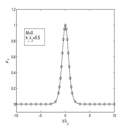
Figure 1: Plot of $\rho_{1}$ against $z/\lambda_{J}$ for $M=0$ and $k_{\perp}\lambda_{J}=0.5$ with the continuous line showing the numerical solution of Eq. (20) and the ‘o’ line indicating the corresponding analytical solution.

Fig. 2 shows the growth rate $\gamma/\omega_{J}$ plotted against $k_{\perp}\lambda_{J}$ as obtained from Eq. (22) as well as from the numerical solution of Eq. (20).

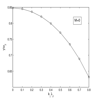
Figure 2: Normalized Jeans instability growth rate for $M=0$ as a function of $k_{\perp}\lambda_{J}$. The continuous line indicates the numerical solution while ‘o’ line indicates the growth rate obtained from exact analytical result.

It is already mentioned that for non zero values of $M$, an exact analytical solution of Eq. (19)is not possible. It is found that the normalized solution of Eq. (19), $\hat{\rho_{1}}$ has the nature of a $\mbox{sech$\,$}{\hat{z}}$ profile and can be fitted with an analytical profile of the form $(\mbox{sech$\,$}\hat{z})^{\alpha}$ with $\alpha$ depending on the value of $M$. In Fig 3 (a), we have shown the $\hat{\rho}_{1}$ profile for $M=0.4$ with $k_{\perp}\lambda_{J}=0.5$ for the growing mode. together with an analytical fit with $\mu=0.52$. In fig. 3(b) we have plotted the corresponding unnormalized solution $\rho_{1}$ against $z/\lambda_{J}$.

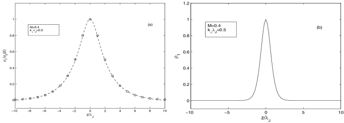
Figure 3: (a) Plot of $n$ against $z/\lambda_{J}$ for $M=0.4$ and $k_{\perp}\lambda_{J}=0.5$ with ‘—’ line showing the normalized solution $\hat{\rho}_{1}$ and the ‘o’ line representing a $(\mbox{sech$\,$}\hat{z})^{0.52}$ profile (b) Plot of $\rho_{1}$ with the same parameters as used in (a).

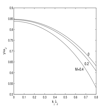
Figure 4: Normalized Jeans instability growth rate for different values of $M$ as a function of $k_{\perp}\lambda_{J}$.

The growth rates for different values of $M$ are shown plotted against $k_{\perp}\lambda_{J}$, showing that with increase in values of $M$, the growth rate decreases.

We also attempt to obtain an approximate solution for Eq. (19). Let us consider $\xi=\tanh\hat{z}$ and take $\xi\ll 1$ so that higher powers of $\xi$ can be neglected,

$$\frac{{\textstyle d^{2}\/n}}{{\textstyle d\/\xi^{2}}}-2\xi\left(\frac{M^{2}+2}{M^{2}+1}\right)\frac{{\textstyle d\/n}}{{\textstyle d\/\xi}}+\left[\frac{2+2\overline{\omega}^{2}-{k}_{\perp}^{2}\lambda_{J}^{2}(1+M^{2})]}{(1+M^{2})}\right]n=0$$ (23)

To solve this equation we can use the transformations

$$n=N(\xi)e^{\int\frac{M^{2}+2}{M^{2}+1}\xi d\xi}~{}~{}{\rm{and}}~{}~{}\bar{\xi}=\xi\sqrt{\frac{M^{2}+2}{M^{2}+1}}$$ (24)

then Eq. (23) reduced to the well known Hermite’s equation

$$\frac{{\textstyle d^{2}\/N}}{{\textstyle d\/\bar{\xi}^{2}}}+\left[\frac{M^{2}+4+2({\omega}^{2}/{\omega_{J}^{2}})-k^{2}_{\perp}\lambda_{J}^{2}(1+M^{2})}{M^{2}+2}-\bar{\xi}^{2}\right]N=0.$$ (25)

The solutions of the Hermite equations are found as $N(\bar{\xi})=\exp{(-\frac{\bar{\xi}^{2}}{2})}H_{\nu}(\bar{\xi})$ where $H_{\nu}$ is a Hermite polynomial. A physically acceptable solution can only be found if it satisfies the dispersion relation

$$\frac{M^{2}+4+2({\omega}^{2}/{\omega_{J}}^{2})-k^{2}_{\perp}\lambda_{J}^{2}(1+M^{2})}{M^{2}+2}=2\nu+1$$ (26)

Different solutions can be obtained for different values of $\nu$. For $\nu=0$, we get back homogeneous density dispersion relation $\omega^{2}=-\omega^{2}_{J}+k_{\perp}^{2}c_{s}^{2}(1+M^{2})$. For $\nu=1$, we obtain the dispersion relation $\omega^{2}=\left(1+M^{2}\right)\left(k_{\perp}^{2}c^{2}_{s}+\omega^{2}_{J}\right)$ that is satisfied for real values of $\omega$ for any value of the wavenumber. Similar results are obtained for all higher values of $\nu$ showing that there is only one mode corresponding to $\nu=0$ that gives rise to imaginary eigenvalues and the instability disappears for higher mode numbers. This feature is also reflected from the numerical analysis of Eq.(19) where only one mode was found to be unstable.

IV Conclusions

A study of Jean’s instability has been carried out for a viscoelastic fluid that exhibits effects of both viscosity and elasticity using generalized hydrodynamic equations of motion. For a Newtonian fluid it is well known that self-gravity leads to an instability for all wavenumbers $k<4\pi G\rho_{0}/c_{s}^{2}$. For a viscoelastic fluid, the upper limit of wavenumber, upto which the gravitational instability is observed is lowered. For a given value of perpendicular wavenumber, the growth rate is shown to decrease with increase in the values of elastic modulus coefficients. Such results have been obtained both for the idealized uniform density case as well as for a one-dimensional equilibrium density profile of the $\mbox{sech$\,$}^{2}$ form. These results may be relevant for stellar matter that is known to exhibit viscoelastic behaviour.

References

- (1) J.H. Jeans, Astronomy and Cosmology (Cambridge University Press, Cambridge, 1929).
- (2) P. K. Shukla and L. Stenflo, Proc. R. Soc. A 462, 403 (2006).
- (3) R. Bingham and V.N. Tsytovich, Astron Astrophys. 376, L43 (2001).
- (4) P. K. Shukla and L. Stenflo, Phys. Lett. A 355 378 (2006).
- (5) H. Ren, Zhengwei Wu, J. Cao and P. K. Chu, Phys. Plasmas 16, 072101 (2009), Zhengwei Wu, H. Ren, J.Cao, and P. K. Chu, Phys. Plasmas, 17, 064503 (2010).
- (6) F. Verheest and V.V. Yaroshenko, Phys. Rev. E 65, 036415 (2002).
- (7) N.F. Cramer and F. Verheest, Phys. Plasmas 12, 082902 (2005).
- (8) S.I. Bastrukov, F. Weber and D.V. Podgainy, J. Phys. G 25 107 (1999).
- (9) Y.I. Frenkel, Kinetic Theory of Liquids (Clarendon, Oxford, 1946).
- (10) P.K. Kaw and A. Sen, Phys. Plasmas 5, 3552 (1998).
- (11) D. Banerjee, M.S. Janaki and N. Chakrabarti, Phys. Plasmas 17, 113708, 2010.
- (12) S. Chandrasekhar, Hydrodynamic and Hydrostatic Stability (Clarendon press, Oxford, 1961).
- (13) W. Fricke, Astrophys. J 120, 356, 1954.