Shear Waves in an inhomogeneous strongly coupled dusty plasma

Abstract

The properties of electrostatic transverse shear waves propagating in a strongly coupled dusty plasma with an equilibrium density gradient are examined using the generalized hydrodynamic equation. In the usual kinetic limit, the resulting equation has similarity to zero energy Schrodinger’s equation. This has helped in obtaining some exact eigenmode solutions in both cartesian and cylindrical geometries for certain nontrivial density profiles. The corresponding velocity profiles and the discrete eigenfrequencies are obtained for several interesting situations and their physics discussed.

I Introduction

In a dusty plasma, the interaction energy between neighbouring dust particles is often much larger than their thermal energy, leading to strong correlation effects between them. This leads to the dust species to exist in a strongly coupled state with a coupling parameter $\Gamma=(Z_{d}e)^{2}/aT_{d}>1$, where $Z_{d}e$, $T_{d}$ are the charge, temperature of the dust grain and $a$ is the distance between the dust grains. The propagation of collective modes in a plasma is influenced by the strong correlation effects between dust particles and the dispersion relations can be studied using the generalized hydrodynamics modelkn:berk -kn:kaw that is appropriate for studying wave motions in the long wave length limit. For a strongly coupled dusty plasma still existing in a fluid state, the existence of a novel transverse shear mode supported by solid-like rigidity of the medium has been predictedkn:kaw and also experimentally verified. Molecular dynamics simulations carried out by Ohta and Hamaguchikn:ohta have identified such shear modes in the fluid phase of Yukawa systems and obtained dispersion relations that are in reasonably good agreement with theoretical estimates. In a medium with inhomogenous charge distribution, the shear modes have been found to be driven unstablekn:sorasio through the dynamics of dust charge fluctuationskn:am . Another important outcome arising out of the inhomogeneous effect is the coupling of the shear and compressional modes that can exploited to find new mechanisms for excitation of shear modes. Such coupling also existskn:yaro among the longitudinal and transverse dust lattice modeskn:nuno and arises due to equilibrium dust charge gradients and particle wake-interactions leading to a dust lattice mode instability. In a non-Newtonian fluid, a coupling between inhomogeneous viscous force and viscosity gradient leads to another novel instability of the transverse shear modekn:debabrata . In a two dimensional complex plasma, viscoelastic vortical flows covering a wide scale of spatial and temporal scales have been observedkn:ratyn and the driving mechanism for such vortex formation is thought to be the charge inhomogeneity across such layer.

In the present work, we attempt to study the propagation of linear transverse shear modes propagating in a strongly coupled dusty plasma having a density gradient in the plane of propagation of the waves. The plasma is considered to be incompressible so as to study the effects of density inhomogeneity on the dispersion characteristics of the shear modes in the absence of any coupling to the acoustic modeskn:am .

II Basic Equations

In a dusty plasma consisting of electrons, ions and dust particles, the charged dust component can easily go into the strongly coupled regime with large values of $\Gamma$ because of the large charge on the dust grains and/or small values of dust temperature while the electrons and ions are in the weakly coupled regime. In the regime $1<\Gamma<\Gamma_{c}$ ($\Gamma_{c}$ is the critical value beyond which crystallization sets in), the medium exhibits both viscous and elastic properties and is known as a viscoelastic medium. An intrinsic feature of viscoelastic media is to exhibit the memory of accumulated shear strain showing viscous effects on long time scales but elastic on short-time scales. The elementary concepts of viscosity and elasticity can be combined in a number of ways to obtain model equations describing viscoelastic fluids. Maxwell model of viscoelasticitykn:bird links the elastic part of stress to strain via an exponentially decaying memory function. A simple generalizationkn:frenkel of the Navier Stokes equation for an incompressible fluid taking into account Maxwell’s relaxation elasticity consists in replacing the normal viscosity coefficient $1/\eta$ by a viscoelastic operator $(1+\tau_{m}d/dt)/\eta$ leading to a generalized momentum equation of hydrodynamics given by

$$\left(1+\tau_{m}\frac{d}{dt}\right)\left[\rho_{d}\frac{d{\bf u_{d}}}{dt}+\nabla p_{d}-Z_{d}en_{d}{\bf E}\right]=\eta\nabla^{2}{\bf u}_{d}$$ (1)

where the convective derivative $d/dt\equiv\partial/\partial t+{\bf u}_{d}\cdot\nabla$. Here $\rho_{d}(=m_{d}n_{d})$ , ${\bf u}_{d}$ and $Z_{d}e$ are the dust mass density, fluid velocity and charge respectively, $p_{d}$ is the dust pressure, $n_{d}$ is the number density, $\bf E$ is the electric field, $\eta$ is the shear coefficient of viscosity, $\tau_{m}$ is the viscoelastic relaxation time that accounts for memory effects. The above equation takes into account the shearing elasticity of the incompressible fluid, which though negligible for small values of $\eta$, becomes an important factor for large values of viscosity when solid like correlations begin to appear in the medium. A more general model applicable to a compressible fluid and involving both bulk and shear moduli is obtainedkn:berk ,kn:kaw by considering a nonlocal viscoelastic operator. For $\tau_{m}=0$, equation(1) reduces to the standard Navier-Stokes hydrodynamic equation. The generalized hydrodynamic model is known to support propagation of undamped transverse shear modes in the kinetic limit characterized by wave frequencies $\omega\gg 1/\tau_{m}$. In order to study such modes, we take the curl of the linearized momentum equation (1) considering an incompressible plasma ( $\nabla\cdot{\bf u}_{d}=0$), to obtain

$$\tau_{m}\frac{\partial^{2}}{\partial t^{2}}\nabla\times(\rho_{d}{{\bf u}_{d}})=\eta\nabla^{2}(\nabla\times{\bf u}_{d})$$ (2)

While deriving the above equation, electrostatic approximation has been assumed. This assumption is justified for the low frequency modes being considered here. For a two dimensional incompressible plasma, $\nabla\cdot{\bf u}_{d}=0$ implies the solution for the velocity as ${\bf u}_{d}={\hat{e}}_{z}\times\nabla\psi(x,y)$, where $\psi(x,y)$ is velocity potential with $\nabla\times{\bf u}_{d}={\hat{e}}_{z}\nabla^{2}\psi$. For an inhomogeneous plasma with $\rho_{d}=\rho_{0d}f({\bf r})$, we obtain from equation(2)

$$\nabla^{4}\psi+\gamma^{2}f\nabla^{2}\psi+\gamma^{2}\nabla f\times({\hat{e}}_{z}\times\nabla\psi)=0,\\$$ (3)

where $\gamma^{2}={\omega^{2}}/{c_{sh}^{2}}\;$ ,$\;c_{sh}^{2}={\eta}/{\rho_{0d}\tau_{m}}$, and $\rho_{0d}$ is the constant dust density. An estimate kn:kaw of $c_{sh}$ obtained from one component plasma limit with the bulk viscosity coefficient neglected in comparison to shear viscosity coefficient is given by

$$c_{sh}^{2}=3\frac{T_{d}}{m_{d}}\left(1-\gamma_{d}\mu_{d}+\frac{4}{15}u\right)$$

where $\gamma_{d}$ is the adiabatic index, $\mu_{d}$ is the compressibility and $u$ is the excess internal energy of the system given by $u(\Gamma)=-0.89\Gamma+0.95\Gamma^{1/4}+0.19\Gamma^{-1/4}-0.81$.

For a uniform plasma, the governing equation describing the propagation of shear modes is given by $\nabla^{2}(\nabla^{2}\psi+\gamma^{2}\psi)=0$ that gives the following dispersion relation describing transverse shear modes:

$$\omega^{2}=k^{2}c_{sh}^{2}$$ (4)

where $c_{sh}$ describes the propagation velocity of the transverse shear mode.

Equation(3) can be solved for various equilibrium density profiles to obtain the eigen-solutions and eigenvalues. A nonlinear model for dust vortex flows using the GH equation has been shownkn:shukla to admit several kinds of vortex structures including the classical dipolar vortex solution. It can be shown that for a special choice of equilibrium density profiles of the following form

$$f(r)=1+\exp\left[\int\frac{J_{1}(\gamma r)}{J_{1}^{\prime}(\gamma r)}d(\gamma r)\right]$$

(where $J$’s are Bessel functions of the first kind and the prime indicate derivative with respect to the arguments) the standard dipole vortex solutions $\psi(r,\theta)=J_{1}(\gamma r)cos\theta$ kn:nc for the shear modes satisfying the equation $\nabla^{2}\psi+\gamma^{2}\psi=0$ can be recovered.

III Shear modes in an Inhomogeneous Plasma

For a plasma with nonuniform density, solutions of equation(3) can be obtained by solving the following equation

$$(\nabla^{2}+\gamma^{2}f)\nabla\psi=\nabla g$$ (5)

for appropriately chosen functional forms for the density profile $f$, as well as $g$, where, for a uniform plasma, $\nabla g$ describes the transformation to a moving frame of reference such that ${\bf u_{d}^{\prime}}={\bf u_{d}}-{\hat{e}_{z}}\times\nabla g$, with $g$ satisfying the equation $\nabla^{2}g=0$. Nontrivial solutions for $g$ lead to an inhomogeneous term in equation (5) that is in general difficult to solve. Throughout the present work, we shall consider $g=0$ and observe that equation(5) has an analogy to Schrodinger’s equation with zero energy and the density profile representing the potential. We shall solve equation(5) for a few cases of specific interest. The case of a uniform plasma is recovered in the limit $f=1$.

(A) Firstly, we consider the propagation of shear waves in one dimension with ${\bf u_{d}}=u_{y}(x){\hat{e}_{y}}$ and density variation $f(x)=\mbox{sech$\,$}^{2}(\alpha x)$ where $\alpha$ is the inverse of characteristic scale length of the density inhomogeneity. The chosen density profile is similar to a Gaussian profile that is observed in plasmas mostly controlled by diffusion process and has the advantage that exact solutions can be obtained for such a profile The eigen-values of equation(5) are obtained as

$$\gamma^{2}=\frac{\omega^{2}}{c_{sh}^{2}}=n(n+1)\alpha^{2}$$ (6)

where $n=1,2,3\cdots$. The corresponding eigenstates for $n=1,2$ kn:lekner are given by

$$u_{y}(x) = u_{y0}\tanh(\alpha x),\;\;\;\;\;\;\;\;\;\;\;\;\;\;\;\;\;\;\;\;\;\;\;\;\;\;\;\;\quad\frac{\omega^{2}}{c_{sh}^{2}}=2\alpha^{2}$$

$$u_{y}(x) = u_{y0}\left[\mbox{sech$\,$}^{2}\left(\alpha x\right)-2\tanh^{2}\left(\alpha x\right)\right],\quad\frac{\omega^{2}}{c_{sh}^{2}}=6\alpha^{2}$$ (7)

that correspond to localized solution.

(B)Next, a two dimensional extension to case (A) can be obtained by considering ${\bf u_{d}}=u_{y}(x,y){\hat{e}_{y}}$, with $f(x,y)=\mbox{sech$\,$}^{2}(\alpha y)$. Regular solutions to the inhomogeneous shear wave equation (5) can be obtained kn:makowski only if the mode frequencies are discrete with $\gamma^{2}$ given by

$$\gamma^{2}_{ns}=\frac{\omega^{2}}{c_{sh}^{2}}={(s+n\pi)(s+n\pi+1)}\alpha^{2},~{}~{}{\rm{with}}~{}~{}s=0,1,2..,n=1,2,3,\cdots$$ (8)

The value of $\omega/c_{sh}$ is determined by the sum $s+n\pi$ with the lowest value given by $\pi$ and the subsequent values given by $1+\pi,2+\pi,.$. For each such value of frequency, we get a corresponding shear mode eigenfunction. The solutions for the velocity component $u_{y}(x,y)=-\partial\psi/\partial x$ are obtained as

$$u_{y}^{n,s}(x,y)=N_{ns}\sqrt{2\alpha}\frac{\sin{n\pi\alpha x}}{(\cosh\alpha y)^{n\pi}}\;G_{s}^{\textstyle{n\pi+\frac{1}{2}}}\tanh\alpha y,$$ (9)

where $G_{s}^{n\pi+1/2}$ is a Gegenbauer polynomial, $N_{ns}$ is a normalization constant. The velocity profiles and the dispersion relations for a few cases are given below

$$u_{y}^{1,0} = N_{10}\sqrt{2\alpha}\sin{\pi\alpha x}(\mbox{sech$\,$}\alpha y)^{\pi},\;\;\;\;\;\;\quad\frac{\omega^{2}}{c_{sh}^{2}}={\pi(\pi+1)}\alpha^{2}$$

$$u_{y}^{1,1} = N_{11}\sqrt{2\alpha}\left(\pi+\frac{1}{2}\right)\sin{\pi\alpha x}(\mbox{sech$\,$}\alpha y)^{\pi}\tanh\alpha y,\;\;\;\;\;\;\quad\frac{\omega^{2}}{c_{sh}^{2}}={(1+\pi)(2+\pi)}\alpha^{2}$$

$$u_{y}^{1,2} = N_{12}\sqrt{2\alpha}\left(\pi+\frac{1}{2}\right)\sin{\pi\alpha x}(\mbox{sech$\,$}\alpha y)^{\pi}\left[2\left(\pi+\frac{3}{2}\right)\tanh^{2}\alpha y-1\right],\quad\frac{\omega^{2}}{c_{sh}^{2}}={(2+\pi)(3+\pi)}\alpha^{2}$$

where

$$N_{10}^{2}=\alpha\frac{\Gamma(\pi+1/2)}{\sqrt{\pi}\Gamma(\pi-1/2)},N_{11}^{2}=\frac{N_{10}^{2}}{2(\pi+1/2)},N_{12}^{2}=\frac{N_{10}^{2}}{2(\pi+1/2)(\pi+1)}$$

Figure 1: Velocity potential contours in the x-y plane for $s=0,n=1$

Figure 2: Velocity potential contours in the x-y plane for $s=1,n=1$

Figure 3: Velocity potential contours in the x-y plane for s=2,n=1

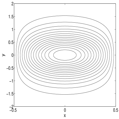
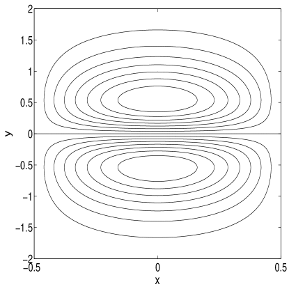
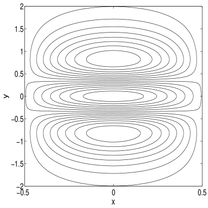
Equation(LABEL:s2) shows that for a density gradient in the $y-$ direction, we obtain periodic solutions in the x-direction, with localization in the y-direction. The solutions corresponding to $n=1,s=0,1$ give rise to monopole and dipole vortices respectively while the solution for $n=1,s=2$ represents a tripolar vortex. The corresponding velocity potential contours are shown in figs.1-3. The number of vortex structures in the figure grows as $s+1$ with the maximum value of velocity potential lying at $x=0$ in each case.

(C) Finally, we consider a cylindrical plasma, with an equilibrium density profile given by $f(r)=(1-\alpha^{2}r^{2})$. In cylindrical coordinates, we get a coupled system of two equations for the components $u_{r}$ and $u_{\theta}$ that are not easy to solve. However, equation(5) can be solved for the two scalars, namely the cartesian components $u_{j},(j=x,y)$ of the velocity vector ${\bf u}$, as functions of $r,\theta$ with the equation expressed in cylindrical coordinates with $z-$ symmetry. The components $u_{r},u_{\theta}$ can be expressed in terms of $u_{x},u_{y}$. Making the substitution $u_{j}(r,\theta)=\chi(r)\exp(im\theta)$ in equation(5), we obtain

$$\frac{1}{r}\frac{\partial}{\partial r}\left(r\frac{\partial\chi}{\partial r}\right)-\frac{m^{2}}{r^{2}}\chi+\gamma^{2}(1-\alpha^{2}r^{2})\chi=0$$ (11)

A physically well-behaved solution of equation(5) is obtained in the form

$$u_{j}(r,\theta)=(\alpha r)^{m}e^{-\gamma\alpha r^{2}/2}{{}_{1}}F_{1}\left(\frac{1+m}{2}-\frac{\gamma}{4\alpha},1+m;{\gamma\alpha r^{2}}\right)\cos{m\theta}$$ (12)

Figure 4: Eigenfunctions obtained for m=1,2,3 with $\omega/c_{sh}\alpha=4.62,6.52,8.42$ respectively.

where ${}_{1}F_{1}(a,b,x)$ is a Kummer confluent hypergeometric function. The physically acceptable solutions are obtained by considering that $\chi(r)$ vanishes at $r=0,r\alpha=1$. This leads to the velocity profiles vanishing at the axis and at the boundary. These conditions give the eigenfrequencies of the shear waves. For each frequency, we obtain two different types of eigenfunctions with different symmetries. For the choice, $u_{y}=0$, we obtain the flow lines situated in the plane $y=$constant and the components of ${\bf u}$ are obtained as

$$u_{r}(r,\theta)=(\alpha r)^{m}e^{-\gamma\alpha r^{2}/2}{{}_{1}}F_{1}\left(\frac{1+m}{2}-\frac{\gamma}{4\alpha},1+m;{\gamma\alpha r^{2}}\right)\cos\theta\cos{m\theta}$$

$$u_{\theta}(r,\theta)=(\alpha r)^{m}e^{-\gamma\alpha r^{2}/2}{{}_{1}}F_{1}\left(\frac{1+m}{2}-\frac{\gamma}{4\alpha},1+m;{\gamma\alpha r^{2}}\right)\sin\theta\cos{m\theta}$$ (13)

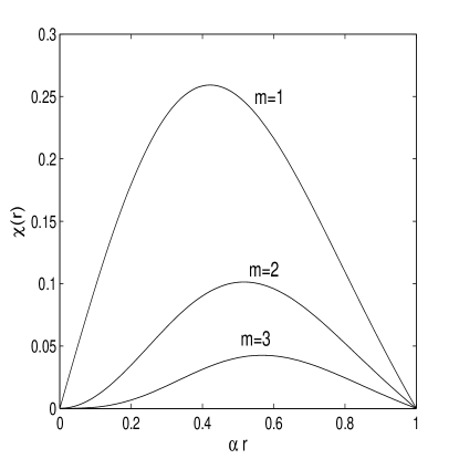
For the parabolic density profile chosen here, the radial part of eigenfunctions, $\chi(r)$ situated in the plane $y=constant$ are shown in fig. 4. The corresponding eigenfrequencies $\omega/c_{sh}\alpha$ are given by $4.62$, $6.52$, $8.42$ for $m=1,2,3$ respectively. For higher poloidal mode numbers, the peak of the radial part of the eigenfunctions shifts towards the plasma edge. A different choice ($u_{x}=0,u_{y}\neq 0$) will yield eigenmodes with the corresponding symmetry. Various kinds of profiles in the $r-\theta$ plane can be generated depending on the values of constants that determine the functional form of the Kummer function.

IV Summary

In this work we have investigated the properties of shear waves in an inhomogeneous plasma where gradients in plasma density are present. The equation governing the velocity potential is identical to zero energy Schrodinger’s equation with the density profile playing the role of potential. The role of inhomogeneity is shown to give rise to a discrete set of allowed frequencies. For a one dimensional model, in presence of a density gradient in the direction of propagation, localized shear modes are obtained in contrast to the freely propagating modes with the allowed mode frequencies depending on the inhomogenity scale length. Shear modes propagating in two dimensions with a density profile that is constant in the x-direction and ${sech^{2}}$ type in the y-direction are shown to admit multipolar vortex solutions. In a cylindrical bounded geometry, with a parabolic density profile, exact analytical solutions for radial and azimuthal velocity components are obtained in terms of Kummer hypergeometric functions.

References

- (1) M.S. Berkovsky, Phys. Lett. A 166,365 (1992).
- (2) J.P. Boon and S. Yip, Molecular Hydrodynamics, (Mc-Graw Hill, New York, 1980).
- (3) P.K. Kaw and A. Sen, Phys. Plasmas, 5,3552 (1998).
- (4) H. Ohta and S. Hamaguchi, Phys. Rev. Lett. 84,6026 (2000).
- (5) G. Sorasio , P. K. Shukla and D. P. Resendes, N. J. Phys. 5, 81, 2003.
- (6) A. Mishra, P.K. Kaw and A. Sen, Phys. Fluids, 7, 3188 (2000).
- (7) V. V. Yaroshenko, A. V. Ivlev, and G. E. Morfill, Phy. Rev. E 71,046405 (2005).
- (8) S. Nunomura, S. Zhdanov, D. Samsonov, and G. Morfill, Phys. Rev. Lett. 94,045001, 2005.
- (9) D. Banerjee, M.S. Janaki and N. Chakrabarti, N. Jour. Phys. 12, 123031, 2010.
- (10) S. Ratynskaia, K. Rypdal, C. Knapek, S. Khrapak, A. V. Milovanov, A. Ivlev, J. J. Rasmussen, and G. E. Morfill, Phys. Rev. Lett. 96,105010 (2006).
- (11) R. B. Bird, R. C. Armstrong, and O. Hassager, Dynamics of Polymeric Liquids, (Wiley, New York, 1987, vol. 1).
- (12) J. Frenkel, Kinetic Theory of liquids, (Clarendon, Oxford, 1946).
- (13) P.K. Shukla, Phys. Plasmas, 10, 1619 (2003).
- (14) M.S. Janaki and N. Chakrabarti, Phys. Plasmas 17053704(2010).
- (15) J. Lekner, Am. J. Phys. 75, 1151 (2007).
- (16) A.J. Makowski, Annals. Phys. 324,2465 (2009).