The average 0.5–200 keV spectrum of local active galactic nuclei and a new determination of the 2–10 keV luminosity function at $\mathbf{z\approx 0}$

Abstract

The broadband X-ray spectra of active galactic nuclei (AGNs) contains information about the nuclear environment from Schwarzschild radii scales (where the primary power-law is generated in a corona) to distances of $\sim 1$ pc (where the distant reflector may be located). In addition, the average shape of the X-ray spectrum is an important input into X-ray background synthesis models. Here, local ($z\approx 0$) AGN luminosity functions (LFs) in five energy bands are used as a low-resolution, luminosity-dependent X-ray spectrometer in order to constrain the average AGN X-ray spectrum between $0.5$ and $200$ keV. The $15$–$55$ keV LF measured by Swift-BAT is assumed to be the best determination of the local LF, and then a spectral model is varied to determine the best fit to the $0.5$–$2$ keV, $2$–$10$ keV, $3$–$20$ keV and $14$–$195$ keV LFs. The spectral model consists of a Gaussian distribution of power-laws with a mean photon-index $\langle\Gamma\rangle$ and cutoff energy $E_{\mathrm{cut}}$, as well as contributions from distant and disc reflection. The reflection strength is parameterised by varying the Fe abundance relative to solar, $A_{\mathrm{Fe}}$, and requiring a specific Fe K$\alpha$ equivalent width (EW). In this way, the presence of the X-ray Baldwin effect can be tested. The spectral model that best fits the four LFs has $\langle\Gamma\rangle=1.85\pm 0.15$, $E_{\mathrm{cut}}=270^{+170}_{-80}$ keV, $A_{\mathrm{Fe}}=0.3^{+0.3}_{-0.15}$ (90% C.L.). The sub-solar $A_{\mathrm{Fe}}$ is unlikely to be a true measure of the gas-phase metallicity, but indicates the presence of strong reflection given the assumed Fe K$\alpha$ EW. Indeed, parameterising the reflection strength with the $R$ parameter gives $R=1.7^{+1.7}_{-0.85}$. There is moderate evidence for no X-ray Baldwin effect. Accretion disc reflection is included in the best fit model, but it is relatively weak (broad iron K$\alpha$ EW $<100$ eV) and does not significantly affect any of the conclusions. A critical result of our procedure is that the shape of the local $2$–$10$ keV LF measured by HEAO-1 and MAXI is incompatible with the LFs measured in the hard X-rays by Swift-BAT and RXTE. We therefore present a new determination of the local $2$–$10$ keV LF that is consistent with all other energy bands, as well as the de-evolved $2$–$10$ keV LF estimated from the XMM-Newton Hard Bright Survey. This new LF should be used to revise current measurements of the evolving AGN LF in the $2$–$10$ keV band. Finally, the suggested absence of the X-ray Baldwin effect points to a possible origin for the distant reflector in dusty gas not associated with the AGN obscuring medium. This may be the same material that produces the compact 12$\mu$m source in local AGNs.

1 Introduction

The X-ray spectra of active galactic nuclei (AGNs) span nearly three decades in energy and are comprised of many separate components: a power-law with a high energy cutoff (e.g., Mushotzky, Done & Pounds, 1993; Nandra & Pounds, 1994; Reeves & Turner, 2000; Zdziarski, Poutanen & Johnson, 2000; Matt, 2001; Molina, Malizia & Bassani, 2006; Molina et al., 2009; Winter et al., 2009; de Rosa et al., 2012; Rivers, Markowitz & Rothschild, 2013; Vasudevan et al., 2013a), reflection from both distant material and the accretion disc (e.g., Pounds et al., 1990; Nandra & Pounds, 1994; Tanaka et al., 1995; Fabian et al., 2002; Nandra et al., 1997, 2007; Ballantyne, 2010; de la Calle Pérez et al., 2010; Shu, Yaqoob & Wang, 2010; Patrick et al., 2012; Ricci et al., 2013) and, in many cases, a soft excess and/or a warm absorber (e.g., Turner & Pounds, 1989; Reynolds, 1997; Perola et al., 2002; Blustin et al., 2005; Crummy et al., 2006; Scott et al., 2011; Scott, Stewart & Mateos, 2012; Tombesi et al., 2013). The variability properties of the X-ray emission indicate that it is generated from very close to the black hole ($\la 10$–$20$ $r_{g}$, where $r_{g}=GM/c^{2}$ is the gravitational radius of a black hole with mass $M$; e.g., Grandi et al. 1992; McHardy et al. 2006; Uttley 2007; Zoghbi et al. 2013), a size scale so small that the physics of the region can only be investigated by spectroscopy. For example, the slope and cutoff energy of the primary power-law is related to the temperature and optical depth of the Comptonizing corona (e.g., Zdziarski et al., 2000; Petrucci et al., 2001; Molina et al., 2009), and the disc reflection features can probe the space-time of the central black hole and the physical state of the underlying accretion flow (e.g., Fabian et al., 1989; Laor, 1991; Brenneman & Reynolds, 2006, 2009; Miller, 2007; Reynolds & Fabian, 2008; Ballantyne, McDuffie & Rusin, 2011). High quality broadband measurements of the X-ray AGNs are therefore crucial to understanding the physics of the central accretion disc (e.g., Risaliti et al., 2013).

In addition to the study of individual objects, studying how the spectral properties of AGNs vary as a function of luminosity and/or redshift may give potentially valuable insights into the evolution of AGNs and the unified model. Current survey results indicate that the X-ray coronal properties seem to be most dependent on the Eddington ratio and not on the cosmic epoch (Shemmer et al., 2006; Risaliti, Young & Elvis, 2009; Brightman et al., 2013). However, distant reflection, as measured from the equivalent width (EW) of the narrow Fe K$\alpha$ line, has shown evidence for a inverse dependence on the X-ray luminosity (e.g., Iwasawa & Taniguchi, 1993; Bianchi et al., 2007; Shu et al., 2010; Ricci et al., 2013). This effect, if real (Shu et al., 2012), would then be providing a clue on how the distant, potentially Compton-thick material around AGNs is dependent on the central engine, with clear implications for the AGN unified model (Ricci et al., 2013).

The broadband spectral shape of AGNs is also a key ingredient for X-ray background (XRB) models (e.g., Gilli, Comastri & Hasinger, 2007; Treister, Urry & Virani, 2009; Ballantyne et al., 2011; Akylas et al., 2012). It is now known that the XRB between $\approx 2$–$200$ keV is comprised of the integrated observed emission of AGNs across all $z$ and X-ray luminosities. Therefore, modeling the XRB requires knowledge of the broadband spectral shape of AGNs, and how it may change with luminosity and redshift. Uncertainty in the spectral shape, in particular the high-energy cutoff and reflection strength, translates directly into uncertainty in the Compton-thick AGN fractions that are derived from fitting the peak of the XRB spectrum at $\approx 20$–$30$ keV (Akylas et al., 2012). Currently, all XRB models assume a spectral shape with some authors accounting for the observed distribution of photon indices and the apparent decline of reflection strength with luminosity (Gilli et al., 2007; Ballantyne et al., 2011).

Aside from a small number of bright sources observed with BeppoSAX (Matt, 2001), the full energy range of AGN spectra has only been studied by combining observations from different X-ray telescopes that can only focus on a small part of the entire spectrum (e.g., de Rosa et al., 2012; Vasudevan, Mushotzky & Gandhi, 2013b). This approach must deal with the cross-calibration of different instruments and the fact that the various observations are often not performed simultaneously, making the resulting spectrum susceptible to the effects of spectral variability. As a result, while catalogues of the spectral properties of hundreds of AGNs have been published (e.g., Brightman & Nandra, 2011; Scott et al., 2011; Rivers et al., 2013; Vasudevan et al., 2013a), these results are often isolated from one another and a clear picture of the broadband spectral properties of AGNs remains elusive. In this paper, we present a novel approach to measure the average $0.5$–$200$ keV spectrum of local AGNs by using the AGN luminosity function (LF) in four energy bands as a low resolution, luminosity-dependent spectrometer. The advantage of using the LFs in this way is that instrumental and (in some cases) absorption effects have been removed. The LFs are also constructed from observations of many AGNs over timescales $\ga 1$ year, mitigating the effects of variability. Thus, finding the spectral model that can simultaneously fit the AGN LF from $0.5$ to $\approx 200$ keV will provide a relatively unbiased view of the average $z\sim 0$ spectral shape.

In the next section, the methodology, LFs and spectral models that are used in the calculation are described. The results of fitting the LFs are discussed in Section 3, in particular the constraints on the spectral model. Section 4 compares the results to previous works, and discusses the implications on XRB modeling and the origin of the distant reflector. We especially emphasize a new measurement of the local $2$–$10$ keV LF. Finally, the conclusions of this study are summarized in Sect. 5. If applicable, all results in this paper make use of the following cosmological parameters: $H_{0}=70$ km s^-1 Mpc^-1, $\Omega_{\Lambda}=0.7$, and $\Omega_{m}=0.3$.

2 Calculations

2.1 Methodology

Given a broadband AGN X-ray spectral model, $L_{E}$, and a reference LF measured in a specific energy band, $d\Phi/d\log L_{\mathrm{ref}}$, then the LF can be predicted in any other band via

$${d\Phi\over d\log L}=C(L){d\Phi\over d\log L_{\mathrm{ref}}}{\Delta\log L_{\mathrm{ref}}\over\Delta\log L},$$ (1)

where $\log L$ is the luminosity in the new band calculated from integrating $L_{E}$. The factor $C(L)$ can be used to convert LFs that account for the entire AGN population to one that includes only a subset. As is described below, an $C(L)$ factor is needed when calculating the $0.5$–$2$ keV LF for unobscured AGNs.

In this study, various forms of $L_{E}$ are considered and $d\Phi/d\log L$ is calculated in four widely separated energy bands. Chi-squared fitting is then used to determine the best fitting spectral model and the error-bars on the associated parameters.

2.2 Local X-ray Luminosity Functions

The following five measurements of the local AGN LF are used to constrain the average spectral shape of AGNs at $z\approx 0$.

$\bullet$15–55 keV (Ajello et al., 2012)
This LF is derived from the 60 month Swift-BAT survey and consists of 428 AGNs with a median redshift of 0.029. As this LF is derived from the most recent and least biased survey of Compton-thin AGNs in the local Universe, it is used as the reference LF for this study. To ease the comparison with LFs derived from lower-energy observations, we make use of the LF derived solely from Compton-thin AGNs (Ajello et al. 2012; Table 5; third row). This LF is consistent with other measurements of the local LF in similar energy ranges (e.g., Sazonov et al., 2008).

$\bullet$0.5–2 keV (Hasinger, Miyaji & Schmidt, 2005)
These authors published the local LF for Type 1 (i.e., non-obscured) AGNs based on 205 AGNs with $0.015<z\la 0.1$ from the ROSAT Bright Survey. As this LF is for only unobscured AGNs, and the reference $15$–$55$ keV LF includes all Compton-thin AGN, a Type 1 fraction must be specified in order to compare the predicted $0.5$–$2$ keV LF to the observed data. Several surveys indicate that this fraction depends strongly on AGN luminosity (e.g., Ueda et al., 2003; Simpson, 2005; Della Ceca et al., 2008; Hasinger, 2008; Gandhi et al., 2009; Burlon et al., 2011; Assef et al., 2013). The triangles in Fig. 1 plot the Type 2 AGN fraction, $f_{2}$, against the $15$–$55$ keV luminosity measured by Burlon et al. (2011) from the 3-year Swift-BAT survey. Here, $f_{2}$ is defined as the ratio of Compton-thin AGNs with $N_{\mathrm{H}}\geq 10^{22}$ cm^-2 to the total number of AGNs with $N_{\mathrm{H}}<10^{24}$ cm^-2 (i.e., no Compton thick objects).

Figure 1: The triangles plot the AGN obscured fraction assuming no Compton-thick sources, $f_{2}$, versus the 15–55 keV luminosity (Burlon et al., 2011). The solid line shows the fit to these data described by eq. 2. The obscured fractions determined by Brightman & Nandra (2011) are shown as the solid points. These measurements were made as a function of 2–10 keV luminosity, but, given the size of the error-bars, they were not converted to 15–55 keV luminosities for this plot.

The obscured fraction falls sharply with luminosity at both high and low luminosity. The effect at high luminosity is often thought to be a result of radiation pressure eroding the covering factor of the dusty obscuring material (Lawrence, 1991). The significance of the decrease of $f_{2}$ at low luminosities is still tentative, but might indicate that a critical luminosity is needed to produce and sustain a geometrically thick obscuring zone (e.g., Elitzur & Ho, 2009; Müller-Sánchez et al., 2013). The solid line in Fig. 1 plots the following fit to the Burlon et al. (2011) data:

$$f_{2}=0.1\left(\log L-40\right)^{3}\exp(-0.32(\log L-41)^{2}),$$ (2)

where $L$ is the $15$–$55$ keV luminosity. Using the smallest of the two error-bars on each $f_{2}$ data-point gives $\chi^{2}=6.7$ for 6 degrees of freedom (dof). Fig. 1 also shows that the $f_{2}$ fractions measured by Brightman & Nandra (2011) from a 12 $\mu$m selected sample (solid points) are in good agreement with the Swift-BAT results and the best fit model. Eq. 2 is used to calculate the Type 2 AGN fraction when predicting the Type 1 $0.5$–$2$ keV LF (i.e., $C(L)=1-f_{2}$).

The Hasinger et al. (2005) LF is based on AGNs identified as Type 1 via the optical definition (i.e., broad Balmer emission lines), while the Swift-BAT measurements and eq. 2 follow the typical X-ray definition (i.e., obscuring line-of-sight column density $N_{\mathrm{H}}<10^{22}$ cm^-2). Hasinger (2008) argues that the optical definition of an unobscured AGN corresponds to a lower value of $N_{\mathrm{H}}\la 3\times 10^{21}$ cm^-2. Therefore, $C(L)$ computed using Eq. 2 must be corrected for the percentage of AGNs with $3\times 10^{21}$ cm${}^{-2}\la N_{\mathrm{H}}<10^{22}$ cm^-2. The $N_{\mathrm{H}}$ distribution measured by Burlon et al. (2011) is used to make this small (only a 11% reduction) correction.

Finally, Hasinger et al. (2005) corrects the $0.5$–$2$ keV luminosities of the AGN sample for Galactic extinction, but not for any small amounts of intrinsic absorption. Thus, all $0.5$–$2$ keV luminosities are predicted for AGN spectra subject to obscuration with $\log N_{\mathrm{H}}=20,20.5$ and $21$, with weightings given by the Burlon et al. (2011) $N_{\mathrm{H}}$ distribution.

$\bullet$2–10 keV (Shinozaki et al., 2006; Ueda et al., 2011)
The Shinozaki et al. (2006) LF is constructed from 49 AGNs with $z<0.4$ observed by HEAO-1, while the Ueda et al. (2011) LF is produced from 37 sources with $0.002<z<0.2$ detected by MAXI. Both analyses corrected the $2$–$10$ keV luminosities for absorption and are sensitive to Compton-thin AGNs. Interestingly, Ueda et al. (2011) point out a disagreement between the shape of the derived $2$–$10$ keV LF with the one measured by Swift-BAT in the $14$–$195$ keV band. These authors suggest that if the spectral shape of AGNs steepens as luminosity increases then the LFs can be made to agree. A similar inconsistency between the Shinozaki et al. (2006) LF and the $3$–$20$ keV LF was discussed by Della Ceca et al. (2008) who showed that it could not be due to absorption.

$\bullet$3–20 keV (Sazonov & Revnivtsev, 2004)
This LF was constructed from 76 Compton-thin AGNs detected by the RXTE Slew Survey. All but 6 sources are at $z<0.1$. Sazonov & Revnivtsev (2004) defined the LF as the number density per observed luminosity interval, so the Burlon et al. (2011) $N_{\mathrm{H}}$ absorption distribution was applied to our spectral model prior to calculating the $3$–$20$ keV luminosities when predicting this LF. The luminosities of the Sazonov & Revnivtsev (2004) LF are increased by 1.4 to account for an error in the flux conversion (Sazonov et al., 2008).

$\bullet$14–195 keV (Tueller et al., 2008)
This LF is based on 88 non-beamed AGNs detected in the 9-month Swift-BAT survey. The AGNs have a median redshift of $0.017$. Given the high energy range of this survey, no absorption correction was made to the luminosities. Although this LF and the $15$–$55$ keV LF are not strictly independent, the latter LF is derived from a much larger dataset in a different energy range by a different analysis technique. Therefore, we consider these two LFs independent enough to allow chi-squared fitting.

2.3 Model AGN Spectra

The AGN spectral model consists of a power-law with a photon-index $\Gamma$ and a high energy cutoff, $E_{\mathrm{cut}}$, and one or two reflection spectra, denoting distant and accretion disc reflection. AGNs exhibit a range of $\Gamma$ that is roughly normally distributed about some average with a dispersion of $\sigma_{\Gamma}\approx 0.3$ (e.g., Brightman & Nandra, 2011; Scott et al., 2011; de Rosa et al., 2012; Vasudevan et al., 2013a). The mean value of this distribution, $\langle\Gamma\rangle$, is not observed to be correlated with the X-ray luminosity (e.g., Brightman et al., 2013). As the LFs are derived from observations of several AGNs, the spectral model is constructed by Gaussian averaging 11 cutoff power-laws around a central $\langle\Gamma\rangle$ with $\sigma_{\Gamma}=0.3$ and $d\Gamma=0.1$ (i.e., a $\langle\Gamma\rangle=1.9$ model includes contributions from power-laws with $\Gamma=1.4$–$2.4$; e.g., Gilli et al. 2007). The distribution of $E_{\mathrm{cut}}$ remains uncertain (e.g., Molina et al., 2009; Ricci et al., 2011), so, for simplicity, all AGNs are assumed to have the same value of $E_{\mathrm{cut}}$.

Distant reflection is modeled using the ‘pexmon’ model (Nandra et al., 2007) available in XSPEC (Arnaud, 1996). The advantage of this model is that it self-consistently adds the Fe K$\alpha$, Fe K$\beta$, Ni K$\alpha$ lines and the Fe K$\alpha$ Compton shoulder to the reflection continuum accounting for how the strengths of these features depend on $\Gamma$, the inclination angle and the metal abundances. The origin of the distant reflector in AGNs is not understood, but may be connected to the pc-scale obscuring material (this is discussed further in Sect. 4.3). In that case, the inclination angle of the reflector could vary widely between Type 1 and 2 AGNs. To account for this, an angle-averaged reflection spectrum (running from 5 deg to 85 deg in steps of 5 deg) was constructed for every $\Gamma$ and $E_{\mathrm{cut}}$.

This angle-averaged reflection spectrum is then added to each power-law prior to the performing the Gaussian average (the results do not significantly change if the reflection spectra are Gaussian averaged and then added to the averaged power-law spectrum). The $R$ parameter is traditionally used to measure the reflection strength in an AGN spectrum. However, its value only has physical meaning for the case of an isotropic source above a disc. Alternatively, the reflection strength can be investigated by specifying the Fe K$\alpha$ EW, and varying the iron abundance ($A_{\mathrm{Fe}}$, where $A_{\mathrm{Fe}}=1$ for Solar abundances). In this manner, an interesting physical property (the Fe abundance of the distant reflector) can be investigated. Spectral models are constructed with the Fe K$\alpha$ EW set in one of two ways: a constant value of 70 eV, or following the Chandra-derived X-ray Baldwin effect: $\log\mathrm{EW}=1.64-0.11(\log L-44)$ (Shu et al., 2010; Shu et al., 2012). The Baldwin effect is measured as a function of $2$–$10$ keV luminosity, but is nearly identical for the $15$–$55$ keV luminosities employed here. The Anders & Grevesse (1989) abundance set is used throughout this study, and only $A_{\mathrm{Fe}}$ is varied .

It is expected that most AGNs also exhibit a disc reflection component including a relativistically broadened Fe K$\alpha$ line (e.g., Nandra et al., 2007). This reflector will contribute to the overall reflection spectrum and therefore may impact the derived strength of the distant reflector. The disc reflection component is investigated with a relativistically blurred ‘pexmon’ model. The ‘kerrconv’ model (Brenneman & Reynolds, 2006) is used to blur the reflection spectrum, assuming a black hole spin of $0.998$, and a disk that is illuminated from $r_{\mathrm{ISCO}}$ to 400 $r_{\mathrm{ISCO}}$ with an emissivity index of $3$ (ISCO=innermost stable circular orbit). For simplicity, both the ‘kerrconv’ and ‘pexmon’ models have a fixed inclination angle of $60$ deg. As with the distant reflector, the disc model is fixed to give a certain Fe K$\alpha$ EW (relative to the power-law; the narrow Fe K$\alpha$ line is removed when adding the disc spectrum). Since the average broad Fe K$\alpha$ EW is observed to be $\la 100$ eV (e.g., Nandra et al., 2007; de la Calle Pérez et al., 2010; Chaudhary et al., 2012; Patrick et al., 2012), disc reflectors are considered with a Fe K$\alpha$ EW of either 54 eV (Ballantyne, 2010) or 96 eV (Patrick et al., 2012). The disc model has the same $A_{\mathrm{Fe}}$, $\Gamma$ and $E_{cut}$ as the distant reflection and power-law models. As is seen below, the addition of disc reflection at this level has a very small impact on the fits to the LFs, so no further investigation of this component is pursued.

In summary, the spectral model $L_{E}$ is constructed by adding reflection spectra derived from the ‘pexmon’ model to a cutoff power-law. All three components have the same $\Gamma$ and $E_{\mathrm{cut}}$. The strengths of the reflection components are set by fixing the EW of the Fe K$\alpha$ lines to a specific value. The spectra are then Gaussian averaged around a mean $\langle\Gamma\rangle$ and normalized to a specific $15$–$55$ keV luminosity to give the final spectral model. In this way, each $L_{E}$ is determined by 3 parameters: $\langle\Gamma\rangle$, $E_{\mathrm{cut}}$ and $A_{\mathrm{Fe}}$. The model is then used, along with the $15$–$55$ keV LF, to predict the LFs in the $0.5$–$2$ keV, $2$–$10$ keV, $3$–$20$ keV and $14$–$195$ keV bands (Sect. 2.1). The parameters are varied with $\langle\Gamma\rangle=1.7,\ldots,2$ (steps of $0.05$), $E_{\mathrm{cut}}=50,\ldots,450$ keV (steps of $10$ keV), and $A_{\mathrm{Fe}}=0.15,\ldots,2$ (steps of $0.05$), and the model that best fits the observed LFs is determined by calculating the joint $\chi^{2}$ (51 data points, 48 dof). A total of six different $L_{E}$ are considered encompassing all the permutations of the different reflection strengths (including the presence or absence of the disc component). In addition, a $L_{E}$ with no reflection components is constructed to compare against the other, more realistic models. All spectral models are defined from $0.1$ keV to $900$ keV in 1000 logarithimically spaced steps. With this binning the narrow Fe K$\alpha$ line has a width (at the base of the line) of 0.12 keV.

3 Results

Here, we discuss the best fit average AGN spectral model at $z\approx 0$ derived from fitting the local $0.5$–$2$ keV, $2$–$10$ keV, $3$–$20$ keV and $14$–$195$ keV LFs. The uncertainty on each parameter is calculated using the 90% confidence level (C.L.) on the parameter of interest (i.e., a $\Delta\chi^{2}=+2.71$ criterion). All $\chi^{2}$ are calculated using the smallest error-bar on each data-point.

It is interesting to first consider the result for a spectral model constructed just from cutoff power-laws (i.e., no distant or disc reflection). In this very idealized case, the best fit model is $\langle\Gamma\rangle=1.7$ and $E_{\mathrm{cut}}=400$ keV with $\chi^{2}/\mathrm{dof}=144/49=2.94$; a very poor fit. Adding distant reflection to the model, with the Fe K$\alpha$ line following the Baldwin effect, decreases $\chi^{2}$ by 53, with the addition of one additional degree of freedom ($A_{\mathrm{Fe}}$). Therefore, the presence of distant reflection in the average AGN spectrum is highly significant (F-test probability$=3\times 10^{-6}$).

Turning to the six spectral models that incorporate distant and (for four of them) disc reflection, the best fit ($\chi^{2}/$dof$=80.5/48=1.68$) to the four LFs is found for the model with a constant narrow Fe K$\alpha$ EW$=70$ eV (i.e., no Baldwin effect), and weak (broad Fe K$\alpha$ EW$=54$ eV) disc reflection. The best fit parameters are $\langle\Gamma\rangle=1.85\pm 0.15$, $E_{\mathrm{cut}}=270^{+170}_{-80}$ keV, and $A_{\mathrm{Fe}}=0.3^{+0.3}_{-0.15}$ (90% C.L.). The fit to the LFs is shown as the solid lines in Figure 2.

Figure 2: The solid lines plot the X-ray LFs as predicted from the best fit spectral model: no X-ray Baldwin effect, disc Fe K$\alpha$ EW$=54$ eV, $\langle\Gamma\rangle=1.85\pm 0.15$, $E_{\mathrm{cut}}=270^{+170}_{-80}$ keV, and $A_{\mathrm{Fe}}=0.3^{+0.3}_{-0.15}$ (90% C.L.). The joint reduced $\chi^{2}$ of this fit is $1.68$. The $\chi^{2}$ of the individual LFs are indicated in the panels. The presence of disc reflection makes only a minor improvement to the fit, but the addition of the Baldwin effect results in $\Delta\chi^{2}=+9.4$. The data points are from Hasinger et al. (2005) ($0.5$–$2$ keV), Ueda et al. (2011) ($2$–$10$ keV; solid points), Shinozaki et al. (2006) ($2$–$10$ keV; open points), Sazonov & Revnivtsev (2004) ($3$–$20$ keV), and Tueller et al. (2008) ($14$–$195$ keV). In the $0.5$–$2$ keV band, the Type 1 LF is predicted using the $f_{2}$–$L$ relation (eq. 2) and the Burlon et al. (2011) $N_{\mathrm{H}}$ distribution to isolate the fraction of AGNs with $\log N_{\mathrm{H}}\leq 21.5$ (Hasinger, 2008). The dashed lines show the best-fit 2–10 keV LF obtained by ignoring the other 3 bands ($\chi^{2}_{\mathrm{red}}\mathrm{(2-10\ keV)}=0.7$; $\chi^{2}_{\mathrm{red}}\mathrm{(Joint)}=33$; no Baldwin effect, disc Fe K$\alpha$ EW$=54$ eV, $\langle\Gamma\rangle=2$, $E_{\mathrm{cut}}=260$ keV, $A_{\mathrm{Fe}}=0.65$). The $2$–$10$ keV number counts predicted by both $2$–$10$ keV LFs are shown in Fig. 6.

The presence of the disc reflection component is very marginal, and removing it increases $\chi^{2}$ by 0.5, with the other parameters changing within the error-bars. The presence of the Baldwin effect, however, gives a $\Delta\chi^{2}=+9.4$, indicating that strong reflection is preferred over a wide range of AGN luminosities (see Sect. 4.3).

The reduced $\chi^{2}$ of this fit ($1.68$) is relatively high and is, strictly speaking, not an acceptable fit to the data. This is either indicating that the spectral model is not correct or that some of the error-bars in the LFs are underestimated. The $\chi^{2}$ of the model when fit to the individual LFs are indicated in the panels of Fig. 2, and shows that the largest contributions to the joint $\chi^{2}$ are from the $0.5$–$2$ keV and $2$–$10$ keV LFs. Many of the points that make up the $0.5$–$2$ keV LF have small error-bars and show slight offsets from the power-law shape of the reference LF. Changes to how $f_{2}$ is calculated (e.g., using eq. 5 of Burlon et al. 2011) or the $N_{\mathrm{H}}$ distribution makes a negligible difference to $\chi^{2}$ in this band. Any additional spectral components such as a warm absorber or a soft excess would be unable to account for these wiggles in the LF without significant fine-tuning. Therefore, the large $\chi^{2}$ found in the $0.5$–$2$ keV band is a result of small error-bars and peculiar shape of this LF. In contrast, the relatively high $\chi^{2}$ in the $2$–$10$ keV band is simply a result of the fact that the shape of the observed LFs is incompatible with the other three bands. To illustrate this, the dashed lines in Fig. 2 show the predicted LFs when only the $2$–$10$ keV LF was used to constrain the model. While the fit to the $2$–$10$ keV LF is excellent (reduced $\chi^{2}=0.67$), the joint reduced $\chi^{2}=33$. The implications of the new $2$–$10$ keV LF fit is discussed in Sect. 4.2.

Returning to the best fit spectral parameters, Figure 3 plots the 68%, 90% and 95% confidence contours (computed for two parameters of interest) in the $E_{\mathrm{cut}}$-$\langle\Gamma\rangle$ and $A_{\mathrm{Fe}}$-$\langle\Gamma\rangle$ planes.

Figure 3: The 68% (solid), 90% (dotted) and 95% (dashed) confidence contours (computed for two parameters of interest) on the spectral model that gives the best joint fit to the multi-band LFs (Fig. 2). The contours are plotted in the $E_{\mathrm{cut}}$–$\langle\Gamma\rangle$ (left panel) and $A_{\mathrm{Fe}}$–$\langle\Gamma\rangle$ (right panel) planes. The plus signs indicate the location of the best-fit parameters ($\langle\Gamma\rangle=1.85$, $A_{\mathrm{Fe}}=0.3$ and $E_{\mathrm{cut}}=270$ keV).

The contours indicate that the tightest constraints are on $A_{\mathrm{Fe}}$ which is constrained to be sub-solar at the 90% C.L. for any value of $\langle\Gamma\rangle$. As the narrow Fe K$\alpha$ EW was fixed at $70$ eV, this is indicating the presence of strong reflection in the average spectrum. As $\langle\Gamma\rangle$ becomes harder, than the reflection can weaken, and the contours shift upward in the plot. In contrast, the limits on $E_{\mathrm{cut}}$ are relatively wide, which is not surprising given that the $14$–$195$ keV band provides only weak constraints on this parameter.

It is interesting to consider what information in the LFs drives the fit of the spectral shape. To answer this question, all the calculations were repeated omitting the $0.5$–$2$ keV LF from the $\chi^{2}$ fitting and then repeated again with the $3$–$20$ keV LF omitted and the $0.5$–$2$ keV LF reinstated. As these datasets have the smallest error-bars they carry the most power in constraining the model. We find that the $0.5$–$2$ keV LF is crucial to determining $\langle\Gamma\rangle$. This energy band carries little to no information on the reflection strength or the high-energy cutoff, but strongly disfavours $\langle\Gamma\rangle>1.95$ (Fig. 3). Not surprisingly, the $3$–$20$ keV LF is most important in constraining the reflection strength as measured by $A_{\mathrm{Fe}}$. Once this LF was included, the limits on $A_{\mathrm{Fe}}$ improved significantly, which, as seen in Fig. 3, affects the values of $\langle\Gamma\rangle$ and $E_{\mathrm{cut}}$.

4 Discussion

4.1 The average spectrum of local AGNs

The result of our experiment is shown in Figure 4 – an average AGN spectrum that is entirely consistent with the $z\approx 0$ LFs spanning from $0.5$ to $195$ keV.

Figure 4: The average X-ray spectrum of local AGNs as found from fitting the local multi-band X-ray LFs (Fig. 2). The spectral model consists of a Gaussian distribution of power-laws with mean photon index $\langle\Gamma\rangle$, dispersion $\sigma_{\Gamma}=0.3$, and high energy cutoff $E_{\mathrm{cut}}$. A reflection spectrum with the same $\Gamma$ distribution and $E_{\mathrm{cut}}$ was calculated from angle-averaged ‘pexmon’ models (Nandra et al., 2007) and added to the primary power-law so that the Fe K$\alpha$ EW$=70$ eV (Shu et al., 2010). Relativistically blurred disc reflection is added so that the broad Fe K$\alpha$ EW$=54$ eV (Ballantyne, 2010).

The derived $\langle\Gamma\rangle=1.85\pm 0.15$ is consistent with many previous measurements of the mean spectral index from a variety of recent samples (e.g., Shemmer et al., 2006; Molina et al., 2009; Burlon et al., 2011; Brightman & Nandra, 2011; Ricci et al., 2011; Rivers et al., 2013; Vasudevan et al., 2013a, b), but is marginally inconsistent with some others (Scott et al., 2011; de Rosa et al., 2012; Molina et al., 2013). The inconsistent values are found from analyses that did not include reflection, were dealing with non-simultaneous observations, or had low count rate data.

Previous constraints on the mean value of $E_{\mathrm{cut}}$ are poor with values ranging from $\sim 110$ keV to $\sim 300$ keV (e.g., Molina et al., 2009; Ricci et al., 2011). The value derived here ($270^{+170}_{-80}$ keV) is largely consistent with these measurements. Assuming a corona with $\tau\la 1$, this value implies that the average AGN corona temperature is $kT\approx 135^{+85}_{-40}$ keV, consistent with prior measurements (Zdziarski et al., 2000; Molina et al., 2009).

The third parameter determined by our procedure is the relative abundance of Fe in the distant reflector, $A_{\mathrm{Fe}}=0.3^{+0.3}_{-0.15}$. The implication of this value for models of the distant reflector is discussed below (Sect. 4.3), but the reason $A_{\mathrm{Fe}}$ is driven to low values is to produce a strong Compton reflection hump at high energies (recall that our procedure fixes the Fe K$\alpha$ EW). Previous measurements of the reflection strength all involve the $R$ parameter. To compare with the previous results, the fitting procedure was re-run with $R$ as a variable and $A_{\mathrm{Fe}}=1$ (the accretion disc reflector was omitted for this run). A good fit was obtained (reduced $\chi^{2}=1.63$; $\Delta\chi^{2}=-2.08$ compared to the model with variable $A_{\mathrm{Fe}}$) with $R=1.7^{+1.7}_{-0.85}$ (90% C.L.), indicating that, indeed, the average reflection strength seems to be large (the values of $\langle\Gamma\rangle$ and $E_{\mathrm{cut}}$ obtained in this fit are $1.85$ and $220$ keV). This value of $R$ is consistent with earlier measurements (e.g., Molina et al. 2009; Burlon et al. 2011; Vasudevan et al. 2013a, b, but see also Rivers et al. 2013).

Vasudevan et al. (2013b) recently presented the stacked spectrum of a complete sample of 95 Swift-BAT-selected local AGNs in the Northern Galactic Cap. As the individual spectra were not corrected for absorption, the resulting sum had the characteristic $2$–$10$ keV $\Gamma\approx 1.4$ power-law of the XRB spectrum. If the average $z\approx 0$ AGN spectrum of Fig. 4 is accurate, then summing this spectrum over the Ajello et al. (2012) LF [while including the Burlon et al. (2011) $N_{\mathrm{H}}$ distribution and the $f_{2}$–$L$ relation (Fig. 1)] should yield a similar result. Figure 5 shows the result of this experiment where the model was scaled so that the two integrated spectra (solid lines; the Vasudevan et al. (2013b) result is in red) are normalized to be the same at an energy of $\approx 5$ keV.

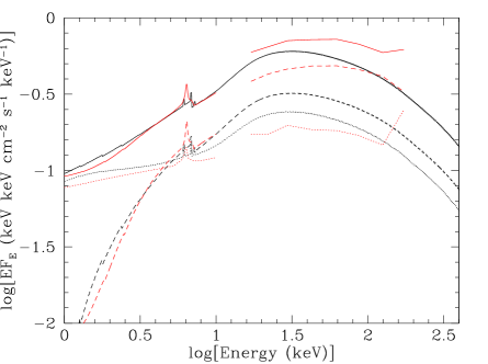
Figure 5: The red lines plot the stacked spectra of 96 Swift-BAT selected local AGNs (Vasudevan et al., 2013b) (solid=all AGNs; dashed=AGNs with $22<\log N_{\mathrm{H}}<24$; dotted=AGNs with $\log N_{\mathrm{H}}<22$). The black lines shows the result of summing the derived local AGNs average spectrum (Fig. 4) over the Ajello et al. (2012) LF while including the absorption distribution. To better compare the shapes of the two spectra, the models were scaled so that the total intensity (solid lines) were equal at $\approx 5$ keV. The $2$–$10$ keV slope of the predicted spectrum is $\Gamma=1.44$, very similar to the observed slope. The contributions from unobscured and Compton-thin obscured AGNs are in good agreement; however, the stacked spectra show stronger reflection in obscured AGNs and moderately weaker reflection in the unobscured AGNs.

In general, the two spectral shapes are in good agreement (the predicted spectrum has $\Gamma=1.44$ in the $2$–$10$ keV band), with the stacked Swift-BAT sources showing a more pronounced hard X-ray hump. The reason for this is found by examining the dotted and dashed lines which plot the contributions from unobscured ($\log N_{\mathrm{H}}<22$) and Compton-thin obscured sources (i.e., $22<\log N_{\mathrm{H}}<24$). Here, one can see that the stacked Compton-thin AGNs show a stronger reflection hump than predicted while the unobscured AGNs present a slightly weaker hump, however, the measured $R$ values agree with the model one within the errors (Vasudevan et al., 2013b). Interestingly, the contributions from obscured and unobscured AGNs agree very well (these lines were not individually adjusted – all three black curves were moved by the same factor to normalize the total) indicating that the Northern Galactic Cap sources well sample the Burlon et al. (2011) $N_{\mathrm{H}}$ distribution. All in all, the agreement of the two spectral shapes seen in Fig. 5 supports the accuracy of our derived spectrum and the effectiveness of the LF-fitting procedure.

4.1.1 Implications for fitting the XRB spectrum

The value of $\langle\Gamma\rangle$ measured here is consistent with the typical value of $1.9$ used by XRB models (e.g., Gilli et al., 2007; Treister et al., 2009; Ballantyne et al., 2011). Similarly, the derived $E_{\mathrm{cut}}$ is also close to the values ($200$–$300$ keV) used in XRB synthesis models. In contrast, there is more variation on the assumption made for the reflection strength: Gilli et al. (2007) and Ballantyne et al. (2011) assume $R\approx 1$ and $A_{\mathrm{Fe}}=1$, but with the reflection strength dropping off with luminosity; alternatively, Treister et al. (2009) use $R=1$ and $A_{\mathrm{Fe}}=2$ at all $L$. This last spectrum has a strong reflection hump and is most similar to the average spectrum measured here. When fitting the XRB spectrum, one must also deal with uncertainties in the evolution of the X-ray LF (Draper & Ballantyne, 2009), the Compton-thick fraction (and its possible evolution; Draper & Ballantyne 2010), and the absorption distribution. These factors, combined with the degeneracies involved in fitting the spectrum (Akylas et al., 2012), means the XRB spectrum can still be fit with an average spectral shape within the measured uncertainties we derived for $\langle\Gamma\rangle$, $E_{\mathrm{cut}}$ and $A_{\mathrm{Fe}}$.

4.2 The 2–10 keV AGN luminosity function

As indicated above, the best multi-band fit to the LFs resulted in a $2$–$10$ keV LF that is not a good representation of the ones measured by HEAO-1 and MAXI. Indeed, as seen in Figure 2, a good fit to the 2–10 keV LF data results in a very poor fit to the $0.5$–$2$ keV and $3$–$20$ keV LFs. Therefore, it appears that the measured local AGN 2–10 keV LF is incompatible with the shape of the LFs determined by Swift-BAT, RXTE and ROSAT.

As this is a surprising result, the $2$–$10$ keV AGN number counts were calculated using the two predicted LFs and spectral models. As these are local LFs, the number counts were only computed for relative bright fluxes. Figure 6 compares the predicted counts to measurements from HEAO-1 (Piccinotti et al., 1982), the XMM-Newton Slew Survey (an extragalactic sample that is $\approx 20$–$25$% galaxies; Warwick, Saxton & Read 2012), and follow-up surveys of Swift-BAT sources (Winter et al., 2009; Vasudevan et al., 2013a).

Figure 6: The solid line plots the 2–10 keV number count predicted by the AGN spectral model derived from the multi-band LF fit, while the dotted line shows the predictions using a spectral model that best fits the local $2$–$10$ keV LF (Fig. 2). The data points are taken from an extragalactic sample from the XMM-Newton Slew Survey (solid triangles; $\approx 80$% AGNs; Warwick et al. 2012), the HEAO-1 AGN sample (open circle; Piccinotti et al. 1982), and follow-up surveys of Swift-BAT selected sources (open squares and stars; Winter et al. 2009 and Vasudevan et al. 2013a, respectively).

Apart from the HEAO-1 point, all these data are entirely independent from those used in the LF fitting and therefore provides a test of the veracity of the predicted LFs. Fig. 6 shows that the LF found from fitting only the $2$–$10$ keV band overpredicts the measured number counts at all fluxes. In contrast, the LF determined from the multi-band fit underpredicts the counts from the XMM-Newton Slew Survey. To determine if an overprediction or underprediction is more likely, we computed the $15$–$55$ keV counts from the adopted $15$–$55$ keV LF (Fig. 7). As the data that comprise the observed $15$–$55$ keV counts were used to measure the LF, the predicted number counts should closely match the observations. Figure 7 shows that the model number counts slightly underpredict the observations, most likely a result of omitting any evolution of the LF and halting the integration at $z=0.2$.

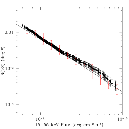
Figure 7: The solid line plots the $15$–$55$ keV number count predicted by the AGN spectral model derived from the multi-band LF fit (Fig. 2). The data points are taken from the 60 month Swift-BAT survey (black points; Ajello et al. 2012), the INTEGRAL measurements by Krivonos et al. (2010) (red crosses; converted to the $15$–$55$ keV band by Ajello et al. 2012). Although we use the $15$–$55$ keV LF described by Ajello et al. (2012), the number counts are slightly underpredicted due to omitting the evolution of the LF. Therefore, the predicted $2$–$10$ keV LF shown in figure 6 will also be slightly below its true value.

Therefore, the predicted $2$–$10$ keV number counts will also be slightly underestimated, which indicates that the model from the multi-band LF fit best describes the observed number counts in the $2$–$10$ keV band. The level of correction implied by Figure 7 will not be enough for the model to exactly match the XMM-Newton Slew Survey data, but these data include a non-negligible fraction of galaxies, and the nature of the slew survey made identification of counterparts difficult at low fluxes (Warwick et al., 2012). Therefore, the measured number counts from this experiment are likely to be slightly too large, especially at low fluxes. Finally, we note that the multi-band fit does overpredict many of the datapoints from Winter et al. (2009) and Vasudevan et al. (2013a), but no error-bars are reported for these measurements, so the degree of mismatch is hard to estimate.

The number counts support the finding that the observed 2–10 keV LFs reported by HEAO-1 and MAXI are incompatible with the shape of the LFs in other energy bands. Fig. 2 shows that the shapes disagree both at the high and low luminosity ends. The high luminosity end is most likely contaminated by AGNs at $z>0.1$ that were included in the ‘local’ sample — the inclusion of these objects would push up the high luminosity end of the LF due to the luminosity evolution of the LF at $z\ga 0.1$ (e.g., Ajello et al., 2012). It is less clear what is causing the overprediction at the low-luminosity end, but it may be related to the small number of AGNs in both samples used to construct the LF. Recall from Sect. 2 that out of the five LFs used here, the 2–10 keV LF measurements were constructed from samples of AGN around half the size of those used in the other bands.

A revision to the local 2–10 keV LF will have important implications in understanding the evolution of AGNs, as it will change the zero-point for all determinations of the evolving LF. To illustrate this, Figure 8 compares the 2–10 keV LF determined by the multi-band fitting (thick black line) to the the $z=0$ LFs predicted by several evolving AGN LFs from the literature (coloured lines).

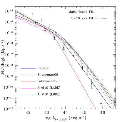
Figure 8: Comparison of the local ($z\approx 0$) 2–10 keV AGN LF determined by the multi-band fit (black solid line) with the LFs published by Ueda et al. (2003), La Franca et al. (2005), Silverman et al. (2008) and Aird et al. (2010) (coloured lines). The black stars plot the de-evolved $z=0$ LF estimated by Della Ceca et al. (2008) from the XMM-Newton Hard Bright Survey. The grey data points are the same as those plotted in Fig. 2. The dotted black line plots the best 2–10 keV LF obtained by our procedure when ignoring the fits to the other three LFs (see also Fig. 2). The 2–10 keV LF obtained by our multi-band approach is strikingly different than the other measurements except for the Della Ceca et al. (2008) estimate.

For reference, the figure also shows the observed 2–10 keV LF as the grey data. This plot clearly shows that every other LF (except for the LADE model of Aird et al. 2010) closely follows the observed 2–10 keV LF, especially at the high luminosity end, and is therefore incompatible with the measured LFs at all other bands. The lone exception is the de-evolved $z=0$ LF estimated by Della Ceca et al. (2008) from the XMM-Newton Hard Bright Survey (black stars) which, although dependent on the model used to de-evolve the LF, is consistent with the multi-band fit at high and low luminosities. It is crucial that the evolution of the AGN LF in the 2–10 keV band be recomputed using the $z=0$ LF reported here (see Table 1) as the zero-point. Once this is done XRB synthesis models will need to be updated in order to revise predictions of the Compton-thick space density at high-$z$ (e.g., Treister et al., 2009; Ballantyne et al., 2011; Akylas et al., 2012).

Table 1: The $2$–$10$ keV LF of $z\sim 0$ AGNs as determined by the multi-band fit (dark solid line in Fig. 8).

$\log L_{\mathrm{2-10\ keV}}$	$\log(d\Phi/d\log L)$
($h_{70}^{-2}$ erg s-1)	($h_{70}^{3}$ Mpc-3)
41.30	$-$3.35
41.56	$-$3.54
41.82	$-$3.73
42.08	$-$3.91
42.34	$-$4.11
42.60	$-$4.30
42.86	$-$4.51
43.12	$-$4.76
43.38	$-$5.07
43.64	$-$5.47
43.90	$-$5.98
44.16	$-$6.54
44.42	$-$7.14
44.68	$-$7.75
44.94	$-$8.36
45.20	$-$8.98
45.46	$-$9.59
45.72	$-$10.21
45.98	$-$10.82
46.24	$-$11.44
46.50	$-$12.06
46.76	$-$12.67
47.02	$-$13.29
47.28	$-$13.90
47.54	$-$14.52
47.80	$-$15.14

4.3 Constraints on the distant reflector

Our procedure also provided interesting constraints on the distant reflector. First, the fits preferred that the reflection strength remain constant as a function of AGN luminosity (e.g., Vasudevan et al., 2013b); that is, the presence of a X-ray Baldwin effect was not required. The strength of any X-ray Baldwin effect has been the source of debate for several years, as it requires precise observations over a wide range of luminosities and being able to control for variability. If present, it might be connected to the obscuring material around the AGN, as Ricci et al. (2013) recently showed that the observed decrease in $f_{2}$ with luminosity could give rise to a Baldwin effect of the right slope. The fact that no Baldwin effect is preferred in the LF fits would indicate that the distant reflector is not associated with the obscuring material, but arises from another source that is common to AGNs of all luminosity, such as the outer regions of the accretion disk or broad-line region clouds (Petrucci et al., 2002; Nandra, 2006; Bianchi et al., 2008). Another intriguing possibility is that the distant reflector is associated with the mid-infrared (12 $\mu$m) emitter that appears to be independent of the X-ray luminosity and AGN classification (Horst et al., 2008; Gandhi et al., 2009; Hönig et al., 2010). Its is also important to remember that both the evidence for and against the X-ray Baldwin effect is concentrated at $2$–$10$ keV luminosities $\la 10^{44}$ erg s^-1; it is still unknown precisely how the reflection strength behaves at larger luminosities.

The average spectrum derived in Sect. 3 strongly indicates that the distant reflector has a sub-solar Fe abundance. Again, the reason the fit was driven to this result was to simultaneously satisfy the constraints of strong reflection and a Fe K$\alpha$ EW of 70 eV. Indeed, the best fitting spectral model that used the $R$ parameter (and found $R=1.7$) predicts a narrow Fe K$\alpha$ EW of 216 eV, much larger than the typical observed values (e.g., Shu et al., 2010). However, a sub-solar Fe abundance in the nuclear environment of AGN host galaxies is problematic, as there is a wealth of evidence that metallicity increases to super-solar abundances in the AGN environment (e.g., Nagao, Marconi & Maiolino 2006 and references therein). Therefore, it is highly unlikely that the abundance $A_{\mathrm{Fe}}=0.3$ found by this procedure is pointing to the true iron abundance. Changing the abundance set to the Lodders (2003) measurement that has a smaller iron abundance does not alter the derived $A_{\mathrm{Fe}}$. Part of the problem may be the geometric assumptions built into the ‘pexmon’ model, as the Compton backscattered and associated line emission are based on an infinitely thick disk geometry. Repeating this experiment with a neutral reflection model that can handle a wider range of geometries (e.g., MYTorus; Yaqoob 2012) would be able to test this assertion, with the limitation of introducing additional free parameters. Alternatively, the low value of $A_{\mathrm{Fe}}$ may indicate that the reflecting medium is dusty. Gas-phase iron is heavily depleted onto grains in dusty gas, but the iron in the grains can still produce Fe K$\alpha$ emission (e.g., Ferland et al., 2013). In this scenario, the EW of the line would depend on the details of the gas-grain mixture as well as geometry, so further investigation of this idea will be the subject of future work. However, this explanation for the value of $A_{\mathrm{Fe}}$ would support the association of the distant reflector with the 12 $\mu$m emitter.

5 Conclusions

This paper presents a measurement of the properties of the average $z\approx 0$ AGN spectrum between $0.5$ and $200$ keV by simultaneously fitting the measured AGN LFs in the $0.5$–$2$ keV, $2$–$10$ keV, $3$–$20$ keV and $14$–$195$ keV bands. The $15$–$55$ keV LF measured by Swift-BAT (Ajello et al., 2012) is used as the best determination of the true $z\approx 0$ LF and the spectral shape was varied to find the best fit to the other four bands. The spectral parameters constrained were the mean photon index of AGNs, $\langle\Gamma\rangle$, the cutoff energy of the power-law, $E_{\mathrm{cut}}$, and the strength of the distant reflector as parameterised by its iron abundance, $A_{\mathrm{Fe}}$. The luminosity dependence of the LFs also allowed a test for the presence of the X-ray Baldwin effect. The principle findings of this study are:

• The best fitting mean AGN spectral model has $\langle\Gamma\rangle=1.85\pm 0.15$, $E_{\mathrm{cut}}=270^{+170}_{-80}$ keV, and $A_{\mathrm{Fe}}=0.3^{+0.3}_{-0.15}$ (90% C.L.). The low iron abundance indicates the need for strong reflection in the average spectrum given the assumed Fe K$\alpha$ EW. The reflection strength is equivalent to $R=1.7^{+1.7}_{-0.85}$ (90% C.L.). The absence of the X-ray Baldwin effect is mildly preferred by the fit ($\Delta\chi^{2}=+9.4$ when the effect is included). These values are consistent with most previous measurements of the average AGN spectrum.

• The shape of the local $2$–$10$ keV AGN LF as measured by HEAO-1 and MAXI is incompatible with LFs measured by Swift-BAT and other instruments. This is likely due to the inclusion of higher $z$ sources in the sample and the small size of the samples. As a result, the evolving $2$–$10$ keV AGN LFs used in XRB modeling need to be revised. The $2$–$10$ keV LF predicted by our procedure is provided in Table 1 and is consistent with the LFs measured in the other bands. This new LF should be used as the zero-point for determining the evolution of the AGN LF in the $2$–$10$ keV band.

• The procedure indicates that strong distant reflection is preferred in local AGNs of all luminosities. That is, we found no evidence of a X-ray Baldwin effect. This result implies that the distant reflector is not associated with the AGN obscuration zone, which does evolve strongly with luminosity. The sub-solar iron abundance may be a result of the assumed disc geometry employed by ‘pexmon’, but may also be indicating that the Fe K$\alpha$ line is emitted by dust grains. If this is the case then the distant reflector must lie outside the dust sublimation zone and may be plausibly associated with the 12 $\mu$m emitter that is observed to be correlated with the X-ray luminosity of all AGNs.

References

- Aird et al. (2010) Aird J. et al., 2010, MNRAS, 401, 2531
- Ajello et al. (2012) Ajello M., Alexander D.M., Greiner J., Madejski G.M., Gehrels N., Burlon D., 2012, ApJ, 749, 21
- Akylas et al. (2012) Akylas A., Georgakakis A., Georgantopoulos I., Brightman M., Nandra K., 2012, A&A, 546, A98
- Anders & Grevesse (1989) Anders E., Grevesse N., 1989, Geochimica et Cosmochimica Acta, 53, 197
- Arnaud (1996) Arnaud K.A., 1996, in Jacoby G., Barnes J., eds, Astronomical Data Analysis Software and Systems V, ASP Conf. Ser. Vol. 101, 17
- Assef et al. (2013) Assef R.J., et al., 2013, ApJ, 772, 26
- Ballantyne (2010) Ballantyne D.R., 2010, ApJ, 708, L1
- Ballantyne et al. (2011) Ballantyne D.R., McDuffie J.R., Rusin, J.S., 2011, ApJ, 734, 112
- Ballantyne et al. (2011) Ballantyne D.R., Draper A.R., Madsen K.K., Rigby J.R., Treister E., 2011, ApJ, 736, 56
- Bianchi et al. (2007) Bianchi S., Guainazzi M., Matt G., Fonseca Bonilla N., 2007, A&A, 467, L19
- Bianchi et al. (2008) Bianchi S., et al., 2008, MNRAS, 389, L52
- Blustin et al. (2005) Blustin A.J., Page M.J., Fuerst S.V., Branduardi-Raymont G., Ashton C.E., 2005, A&A, 431, 111
- Brenneman & Reynolds (2006) Brenneman L.W., Reynolds C.S., 2006, ApJ, 652, 1028
- Brenneman & Reynolds (2009) Brenneman L.W., Reynolds C.S., 2009, ApJ, 702, 1367
- Brightman & Nandra (2011) Brightman M., Nandra K., 2011, MNRAS, 414, 3084
- Brightman et al. (2013) Brightman M., et al., 2013, MNRAS, 433, 2485
- Burlon et al. (2011) Burlon D., Ajello M., Greiner J., Comastri A., Merloni A., Gehrels N., 2011, ApJ, 728, 58
- Chaudhary et al. (2012) Chaudhary P., Brusa M., Hasinger G., Merloni A., Comastri A., Nandra K., 2012, A&A, 537, A6
- Crummy et al. (2006) Crummy J., Fabian A.C., Gallo L., Ross R.R., 2006, MNRAS, 365, 1067
- de la Calle Pérez et al. (2010) de la Calle Pérez I., et al., 2010, A&A, 524, 50
- de Rosa et al. (2012) de Rosa A., et al., 2012, MNRAS, 420, 2087
- Della Ceca et al. (2008) Della Ceca R., et al., 2008, A&A, 487, 119
- Draper & Ballantyne (2009) Draper A.R., Ballantyne D.R., 2009, ApJ, 707, 778
- Draper & Ballantyne (2010) Draper A.R., Ballantyne D.R., 2010, ApJ, 715, L99
- Elitzur & Ho (2009) Elitzur M., Ho L.C., 2009, ApJ, 701, L91
- Fabian et al. (1989) Fabian A.C., Rees M.J., Stella L., White N.E., 1989, MNRAS, 238, 729
- Fabian et al. (2002) Fabian A.C., et al., 2002, MNRAS, 335, L1
- Ferland et al. (2013) Ferland G.J., et al., 2013, Rev. Mex. Ast., 49, 137
- Gandhi et al. (2009) Gandhi P., Horst H., Smette A., Hönig S., Comastri A., Gilli R., Vignali C., Duschl W., 2009, A&A, 502, 457
- Gilli et al. (2007) Gilli R., Comastri A., Hasinger G., 2007, A&A, 463, 79
- Grandi et al. (1992) Grandi P., Tagliaferri G., Giommi P., Barr P., Palumbo, G.G.C., 1992, ApJS, 82, 93
- Hasinger (2008) Hasinger G., 2008, A&A, 490, 905
- Hasinger et al. (2005) Hasinger G., Miyaji T., Schmidt M., 2005, A&A, 441, 417
- Horst et al. (2008) Horst H., Gandhi P., Smette A., Duschl W.J., 2008, A&A, 479, 389
- Hönig et al. (2010) Hönig S.F., Kishimoto M., Gandhi P., Smette A., Asmus D., Duschl W., Polletta M., Weigelt G., 2010, A&A, 515, 23
- Iwasawa & Taniguchi (1993) Iwasawa K., Taniguchi Y., 1993, ApJ, 413, L15
- Krivonos et al. (2010) Krivonos R., et al.., 2010, A&A, 523, A61
- La Franca et al. (2005) La Franca F. et al., 2005, ApJ, 635, 864
- Laor (1991) Laor A., 1991, ApJ, 376, 90
- Lawrence (1991) Lawrence A., 1991, MNRAS, 252, 586
- Lodders (2003) Lodders K., 2003, ApJ, 591, 1220
- Matt (2001) Matt G., 2001, in White N.E., Magaluti G., Palumbo G., eds., X-Ray Astronomy: Stellar Endpoints, AGN, and the Diffuse X-ray Background, Proc. AIP Conf. 599, Am. Inst. Phys., 209
- McHardy et al. (2006) McHardy I.M., Koerding E., Knigge C., Uttley P., Fender, R.P., 2006, Nature, 444, 730
- Miller (2007) Miller J.M., 2007, ARA&A, 45, 441
- Molina et al. (2006) Molina M., Malizia A., Bassani L., 2006, MNRAS, 371, 821
- Molina et al. (2009) Molina M., et al., 2009, MNRAS, 399, 1293
- Molina et al. (2013) Molina M., Bassani L., Malizia A., Stephen J.B., Bird A.J., Bazzano A., Ubertini P., 2013, MNRAS, 433, 1687
- Müller-Sánchez et al. (2013) Müller-Sánchez F., Prieto M.A., Mezcua M., Davies R.I., Malkan M.A., Elitzur M., 2013, ApJ, 763, L1
- Mushotzky et al. (1993) Mushotzky R.F., Done C., Pounds K.A., 1993, ARA&A, 31, 717
- Nagao et al. (2006) Nagao T., Marconi A., Maiolino R., 2006, A&A, 447, 157
- Nandra (2006) Nandra K., 2006, MNRAS, 368, L62
- Nandra & Pounds (1994) Nandra K., Pounds K.A., 1994, MNRAS, 268, 405
- Nandra et al. (1997) Nandra K., George I.M., Mushotzky R.F., Turner T.J., Yaqoob T., 1997, ApJ, 476, 70
- Nandra et al. (2007) Nandra K., O’Neill P.M., George I.M., Reeves J.N., 2007, MNRAS, 382, 194
- Patrick et al. (2012) Patrick A.R., Reeves J.N., Porquet D., Markowitz A.G., Braito V., Lobban A.P., 2012, MNRAS, 426, 2522
- Perola et al. (2002) Perola G.C., et al., 2002, A&A, 389, 802
- Petrucci et al. (2001) Petrucci P.O., et al., 2001, ApJ, 556, 716
- Petrucci et al. (2002) Petrucci P.O., et al., 2002, A&A, 388, L5
- Piccinotti et al. (1982) Piccinotti G., Mushotzky R.F., Boldt E.A., Holt S.S., Marshall F.E., Serlemitsos P.J., Shafer R.A., 1982, ApJ, 253, 485
- Pounds et al. (1990) Pounds K.A., Nandra K., Stewart G.C., George I.M., Fabian A.C., 1990, Nature, 344, 132
- Reeves & Turner (2000) Reeves J.N., Turner M.J.L., 2000, MNRAS, 316, 234
- Reynolds (1997) Reynolds C.S., 1997, MNRAS, 286, 513
- Reynolds & Fabian (2008) Reynolds C.S., Fabian A.C., 2008, ApJ, 675, 1048
- Ricci et al. (2011) Ricci C., Walter R., Courvoisier T.J.-L., Paltani S., 2011, A&A, 532, 102
- Ricci et al. (2013) Ricci C., Paltan, S., Awaki H., Petrucci P.-O., Ueda Y., Brightman M., 2013, A&A, 553, A29
- Risaliti et al. (2009) Risaliti G., Young M., Elvis M., 2009, ApJ, 700, L6
- Risaliti et al. (2013) Risaliti G., et al., 2013, Nature, 494, 449
- Rivers et al. (2013) Rivers E., Markowitz A., Rothschild R., 2013, ApJ, 772, 114
- Sazonov & Revnivtsev (2004) Sazonov S., Revnivtsev M., 2004, A&A, 423, 469
- Sazonov et al. (2008) Sazonov S., Krivonos R., Revnivtsev M., Churazov E., Sunyaev R., 2008, A&A, 482, 517
- Scott et al. (2011) Scott A.E., Stewart G.C., Mateos S., Alexander D.M., Hutton S., Ward M.J., 2011, MNRAS, 417, 992
- Scott et al. (2012) Scott A.E., Stewart G.C., Mateos S., 2012, MNRAS, 423, 2633
- Shemmer et al. (2006) Shemmer O., Brandt W.N., Netzer H., Maiolino R., Kaspi S., 2006, ApJ, 646, L29
- Shinozaki et al. (2006) Shinozaki K., Miyaki T., Ishisaki Y., Ueda Y., Ogasaka Y., 2006, AJ, 131, 2843
- Shu et al. (2010) Shu X.W., Yaqoob T., Wang J.X., 2010, ApJS, 187, 581
- Shu et al. (2012) Shu X.W., Wang J.X., Yaqoob T., Jiang P., Zhou Y.Y., 2012, ApJ, 744, L21
- Silverman et al. (2008) Silverman J.D. et al., 2008, ApJ, 679, 118
- Simpson (2005) Simpson C., 2005, MNRAS, 360, 565
- Tanaka et al. (1995) Tanaka Y., et al., 1995, Nature, 375, 659
- Tombesi et al. (2013) Tombesi F., Cappi M., Reeves J.N., Nemmen R.S., Braito V., Gaspari M., Reynolds C.S., 2013, MNRAS, 430, 1102
- Treister et al. (2009) Treister E., Urry C.M., Virani S., 2009, ApJ, 696, 110
- Tueller et al. (2008) Tueller J., Mushtozky R.F., Barthelmy S., Cannizzo J.K., Gehrels N., Markwardt C.B., Skinner G.K., Winter L.M., 2008, ApJ, 681, 113
- Turner & Pounds (1989) Turner T.J., Pounds K.A., 1989, MNRAS, 240, 833
- Ueda et al. (2003) Ueda Y., Akiyama M., Ohta K., Miyaji, T., 2003, ApJ, 598, 886
- Ueda et al. (2011) Ueda Y. et al., 2011, PASJ, 63, S937
- Uttley (2007) Uttley P., 2007, in The Central Engine of Active Galactic Nuclei, ASP Conference Series, eds. Ho. L.C. & Wang J.-M., Vol. 373, p. 149
- Vasudevan et al. (2013a) Vasudevan R.V., Brandt W.N., Mushotzky R.F., Winter L.M., Baumgartner W.H., Shimizu T.T., Schneider D.P., Nousek J., 2013a, ApJ, 763, 111
- Vasudevan et al. (2013b) Vasudevan R.V., Mushotzky R.F., Gandhi P., 2013b, ApJ, 770, L37
- Warwick et al. (2012) Warwick R.S., Saxton R.D., Read A.M., 2012, A&A, 548, A99
- Winter et al. (2009) Winter L.M., Mushotzky R.F., Reynolds C.S., Tueller J., 2009, ApJ, 690, 1322
- Yaqoob (2012) Yaqoob T., 2012, MNRAS, 423, 3360
- Zdziarski et al. (2000) Zdziarski A.A., Poutanen J., Johnson W.N., 2000, ApJ, 542, 703
- Zoghbi et al. (2013) Zoghbi A., Reynolds C., Cackett E.M., Miniutti G., Kara E., Fabian A.C., 2013, ApJ, 767, 121