Exactly solvable models and bifurcations: the case of the cubic $NLS$ with a $\delta$ or a $\delta^{\prime}$ interaction.

Abstract.

We explicitly give all stationary solutions to the focusing cubic NLS on the line, in the presence of a defect of the type Dirac’s delta or delta prime. The models proves interesting for two features: first, they are exactly solvable and all quantities can be expressed in terms of elementary functions. Second, the associated dynamics is far from being trivial. In particular, the $NLS$ with a delta prime potential shows two symmetry breaking bifurcations: the first concerns the ground states and was already known. The second emerges on the first excited states, and up to now had not been revealed. We highlight such bifurcations by computing the nonlinear and the no-defect limits of the stationary solutions.

1. Introduction

In recent years, the spectacular development of experimental techniques in condensed matter and ultracold gases, has greatly increased the interest in the mathematical modeling of the dynamics of Bose-Einstein condensates, i.e. in the Gross-Pitaevskii equation

$$i\partial_{t}\psi(t,x)\ =\ -\Delta\psi(t,x)\pm\lambda|\psi(t,x)|^{2}\psi(t,x)+V(x)\psi(t,x),\qquad t\in{\mathbb{R}},\,x\in{\mathbb{R}}^{d},\lambda>0$$ (1.1)

where the unknown $\psi(t,\cdot)$ is the wavefunction of the condensate, the potential $V$ models the action of an external field, and the cubic term summarizes the effects of the two-body interactions among the particles in the condensate. It is well-known that the coupling constant $\pm\lambda$ of the nonlinearity is proportional to the scattering length of such a two-body interaction.

The function $V$ can be characterized by the same lengthscale of the condensate, for instance when it models the trap confining the system, or by a much shorter lengthscale, for instance when it describes the effect of an inhomogeneity or of an impurity.

In this paper we focus on the latter case, restrict our study to the so-called cigar-shaped condensates, i.e. effectively one-dimensional systems, and specialize to the choices

$$1.~{}V(x)=-\alpha\delta_{0},\ \alpha>0.\qquad 2.~{}V(x)=-\gamma\delta^{\prime}_{0},\ \gamma>0.$$ (1.2)

While choice 1. can be rigorously described as the action of a delta-shaped potential to be understood in the sense of distributions, the formalization of choice 2. requires to make resort to the self-adjoint extension theory due to Von Neumann and Krein ([5, 4]). Using such theory, one ends up by defining the singluar interactions in (1.2) by means of suitable boundary conditions (see [5, 6]).

In the present paper we consider the equations

$$i\partial_{t}\psi(t)\ =\ H_{j}\psi(t)-\alpha|\psi(t)|^{2}\psi(t),\qquad t\in{\mathbb{R}},\,j=1,2\,,$$ (1.3)

where the hamiltonian operator $H_{1}$ and $H_{2}$ are defined as follows:

• $H_{1}$ is the quantum Hamiltonian operator associated to an attractive Dirac’s delta potential. Its precise definition is the following: given $\alpha>0$,

  $$\begin{split}D(H_{1})\ &:=\ \{\psi\in H^{2}({\mathbb{R}}\backslash\{0\})\cup H^{1}({\mathbb{R}}),\ \psi^{\prime}(0+)-\psi^{\prime}(0-)=\alpha\psi(0+)=\alpha\psi(0-)\}\\ &(H_{1}\psi)(x)\ =\ -\psi^{\prime\prime}(x).\end{split}$$ (1.4)

• $H_{2}$ is the quantum Hamiltonian operator associated to an attractive delta prime potential. Given $\gamma>0$,

  $$\begin{split}D(H_{2})\ &:=\ \{\psi\in H^{2}({\mathbb{R}}\backslash\{0\}),\quad\psi^{\prime}(0+)=\psi^{\prime}(0-),\quad\ \psi(0+)-\psi(0-)=-\gamma\psi^{\prime}(0+)\}\\ &(H_{2}\psi)(x)\ =\ -\psi^{\prime\prime}(x).\end{split}$$ (1.5)

Thinking of the applications to models for BEC, the natural mathematical environment is the energy space. It is widely known (see e.g. [1]) that the energy space for the Dirac’s delta case is

$$Q_{\delta}:=H^{1}({\mathbb{R}})$$ (1.6)

and, given $\psi\in Q_{\delta}$, the related energy functional reads

$$E_{\alpha\delta}(\psi)\ :=\ \frac{1}{2}\int_{\mathbb{R}}|\psi^{\prime}(x)|^{2}\,dx-\frac{\alpha}{2}|\psi(0)|^{2}-\frac{\lambda}{4}\int_{\mathbb{R}}|\psi(x)|^{4}\,dx.$$ (1.7)

On the other hand, for the delta prime interaction the energy space reads

$$Q_{\delta^{\prime}}:=H^{1}({\mathbb{R}}^{+})\oplus H^{1}({\mathbb{R}}^{-}).$$ (1.8)

and, given $\psi\in Q_{\delta^{\prime}}$, the related energy functional reads

$$\begin{split}E_{\gamma\delta^{\prime}}(\psi)\ :=&\ \frac{1}{2}\lim_{\varepsilon\to 0}\left[\int_{-\infty}^{-\varepsilon}|\psi^{\prime}(x)|^{2}\,dx+\int_{\varepsilon}^{+\infty}|\psi^{\prime}(x)|^{2}\,dx\right]-\frac{1}{2\gamma}|\psi(0+)-\psi(0-)|^{2}\\ &\ -\frac{\lambda}{4}\int_{\mathbb{R}}|\psi(x)|^{4}\,dx.\end{split}$$ (1.9)

In [1] it was proven that the problem given by (1.3) is globally well-posed for any initial data in the related energy space. Moreover, $L^{2}$-norm and energy are conserved quantities.

As already stressed, the main focus of the present paper is given by the stationary states of (1.3). We call stationary state any square-integrable solution to the equation (1.3) of the type

$$\psi_{\omega}(t,x)\ =\ e^{i\omega t}\phi_{\omega}(x),\qquad\omega>0.$$ (1.10)

As a consequence, the function $\phi_{\omega}$ must solve the stationary Schrödinger equation

$$H_{j}\phi_{\omega}-\lambda|\phi_{\omega}|^{2}\phi_{\omega}+\omega\phi_{\omega}\ =\ 0,\qquad j=1,2$$ (1.11)

that can be rephrased as the problem of finding a function $\phi_{\omega}$ in the appropriate energy space that satisfies the equation

$$-\phi_{\omega}^{\prime\prime}-\lambda|\phi_{\omega}|^{2}\phi_{\omega}+\omega\phi_{\omega}\ =\ 0,\qquad x\neq 0$$ (1.12)

and fulfils the boundary conditions already given in (1.4) and (1.5):

• in the case of the Dirac’s delta potential

  $$\phi_{\omega}^{\prime}(0+)-\phi_{\omega}^{\prime}(0-)\ =\ -\alpha\phi_{\omega}(0+)\ =\ -\alpha\phi_{\omega}(0-);$$ (1.13)

• in the case of the delta prime interaction

  $$\phi_{\omega}(0+)-\phi_{\omega}(0-)\ =\ -\gamma\phi_{\omega}^{\prime}(0+)\ =\ -\gamma\phi_{\omega}^{\prime}(0-).$$ (1.14)

It is well-known that any $L^{2}$ solution to (1.12) must be of the following type:

$$\phi_{\omega}(x)\ :=\ \left\{\begin{array}[]{c}\sqrt{\frac{2\omega}{\lambda}}\textrm{sech}(\sqrt{\omega}(x-x_{1})),\qquad x<0\\ \\ \sqrt{\frac{2\omega}{\lambda}}\textrm{sech}(\sqrt{\omega}(x-x_{2})),\qquad x>0,\end{array}\right.$$ (1.15)

so the problem of finding stationary states reduces to the issue of determining the parameters $x_{1}$ and $x_{2}$ in order to fulfil the matching condtions (1.13) or (1.14).

In this paper we find all stationary solutions to equation (1.3) for both linear Hamiltonians operators $H_{1}$ and $H_{2}$ and perform two kinds of limit on them: the so-called linear limit, i.e. $\lambda\to 0+$ and the no-defect limit, which amounts to $\alpha\to 0+$ for the Dirac’s delta potential; for the delta prime interaction it is not so immediate to give a notion of no-defect limit, so we study both limits $\gamma\to 0+$, that seems to be justified as a no-defect limit by (1.5), and $\gamma\to+\infty$ that, according to (1.9) seems to be justified as a no-defect limit too.

It is well-known that the standard nonlinear Schrödinger equation in dimension one is a completely integrable system ([16]); adding a perturbation complete integrability is broken but some characters of exact solvability are retained. For example perturbating with a Dirac’s delta interaction, the stationary states of the system can still be exactly computed ([8, 13, 11, 10, 14]). In analogy with these cases, the problem of the stationary states for equation (1.3) with a delta prime interaction proves exactly solvable too. In addition, as shown in [2], the structure of the family of ground states can exhibit non-trivial bifurcations.

The paper is organized as follows: in Section 2 we treat the case of the Dirac’s delta potential, while in Section 3 we study the effect of a delta prime interaction. Comments on the arising bifurcations are given after any theorem.

1.1. Notation

Along with the symbols already introduced for energy spaces and energy functionals, we make use of the following notation:

• The $L^{p}({\mathbb{R}})$-norm of the function $\psi$ is denoted by $\|\psi\|_{p}$. The energy norm is referred to as $\|\psi\|_{Q_{\delta}}$ and $\|\psi\|_{Q_{\delta^{\prime}}}$, for the case with a Dirac’s delta and a delta prime potential, respectively.

• We make use of a family of functionals called action, defined as follows: choose $\omega>0$, then

  $$S_{\omega}(\psi)\ =E(\psi)+\frac{\omega}{2}\|\psi\|^{2}_{2},$$ (1.16)

  where $E$ can be either $E_{\alpha\delta}$ or $E_{\gamma\delta^{\prime}}$ according to the case one is examining.

• For any $A,B>0,C\in{\mathbb{R}}$ we define the function

  $$\phi(A,B,C;x):=A\,\textrm{sech}(Bx-C)$$ (1.17)

1.2. A preliminary lemma

The following lemma provides an estimate that will be repeatedly used along the paper.

Lemma 1.1.

Defined the function $\phi(A,B,C)$ as in (1.17), the following estimate holds:

$$\begin{split}&\ \|\phi(A,B,C)-\phi(A^{\prime},B^{\prime},C^{\prime})\|_{H^{1}({\mathbb{R}}^{+})}\\ \leq&\ c|A-A^{\prime}|\|\textrm{sech}(B\cdot)\|_{H^{1}({\mathbb{R}})}+c|B-B^{\prime}|\|e^{-\min(B,B^{\prime})|\cdot|}\|_{H^{1}({\mathbb{R}})}+c|C-C^{\prime}|\|\textrm{sech}(B\cdot)\|_{H^{2}({\mathbb{R}})},\end{split}$$ (1.18)

where $c$ is a positive constant.

Proof.

By triangular inequality

$$\begin{split}&\|\phi(A,B,C)-\phi(A^{\prime},B^{\prime},C^{\prime})\|_{H^{1}({\mathbb{R}}^{+})}\\ \leq&\ |A-A^{\prime}|\|\phi(1,B,0)\|_{H^{1}({\mathbb{R}})}+|A^{\prime}|\|\phi(1,B,0)-\phi(1,B^{\prime},0)\|_{H^{1}({\mathbb{R}})}\\ &+|A^{\prime}|\|\phi(1,B^{\prime},C)-\phi(1,B^{\prime},C^{\prime})\|_{H^{1}({\mathbb{R}}^{+})}\\ =:&(I)+(II)+(III)\end{split}$$ (1.19)

Term $(I)$ is already in its final form, let us work on $(II)$ and $(III)$.

Concerning $(II)$, notice that

$$|\textrm{sech}(Bx)-\textrm{sech}(B^{\prime}x)|\leq 4|e^{-Bx}-e^{-B^{\prime}x}|\leq 4|B-B^{\prime}|e^{-\min(B,B^{\prime})|x|},$$

thus

$$\|\textrm{sech}(B\cdot)-\textrm{sech}(B^{\prime}\cdot)\|_{2}^{2}\leq 16|B-B^{\prime}|^{2}\|e^{-\min(B,B^{\prime})|\cdot|}\|_{2}^{2}.$$

Analogously,

$$\left|\frac{d}{dx}\left(\textrm{sech}(Bx)-\textrm{sech}(B^{\prime}x)\right)\right|\leq 6|e^{-Bx}-e^{-B^{\prime}x}||B-B^{\prime}|e^{-\min(B,B^{\prime})|x|},$$

then

$$\|\textrm{sech}(B\cdot)-\textrm{sech}(B^{\prime}\cdot)\|_{H^{1}({\mathbb{R}})}\leq c|B-B^{\prime}|\|e^{-\min(B,B^{\prime})|\cdot|}\|_{H^{1}({\mathbb{R}})}$$

Finally, concerning term $(III)$, we observe that

$$\widehat{\phi(1,B^{\prime},C)}(k)-\widehat{\phi(1,B^{\prime},C)}(k)=\frac{e^{-ikC}-e^{-ikC^{\prime}}}{B^{\prime}}\widehat{\textrm{sech}}\left(\frac{k}{B^{\prime}}\right),$$

where $\widehat{f}$ denotes the Fourier transform of the function $f$. Then, a straightforward estimate gives

$$\|\phi(1,B^{\prime},C)-\phi(1,B^{\prime},C)\|_{H^{1}({\mathbb{R}})}^{2}\leq\frac{|C-C^{\prime}|^{2}}{|B^{\prime}|^{2}}\int_{\mathbb{R}}(1+|k|^{2})|k|^{2}\left|\widehat{\textrm{sech}}\left(\frac{k}{B^{\prime}}\right)\right|^{2}\,dk.$$

The proof is complete. ∎

2. Dirac’s delta defect

Here we investigate the stationary states of the system

$$\begin{split}i\partial_{t}\psi(t,x)&\ =\ H_{1}\psi(t,x)-\lambda|\psi(t,x)|^{2}\psi(t,x)\end{split}$$ (2.1)

As shown by several authors ([15, 11, 3]), there exists a unique branch of stationary states that reads

$$\psi_{\alpha\delta,\omega}\ =\ \sqrt{\frac{2\omega}{\lambda}}\textrm{sech}(\sqrt{\omega}(|x|-\bar{x}_{\alpha,\omega}))$$ (2.2)

where

$$\bar{x}_{\alpha,\omega}=\frac{1}{2\sqrt{\omega}}\log\frac{2\sqrt{\omega}-\alpha}{2\sqrt{\omega}+\alpha}.$$

Notice that $\bar{x}_{\alpha,\rho,\lambda}<0$. The typical situation is represented in Figure 1.

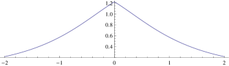
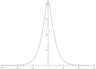
Figure 1. $\psi_{\delta\omega}$ for $\alpha=1$, $\lambda=1$ and $\omega=1$ $\omega=9$.

By direct computation, one has the following results for $L^{2}$-norm, energy and action:

Proposition 2.1.

The $L^{2}$-norm, the energy, and the action of the stationary states given in (2.2) read

$$\begin{split}\|\psi_{\alpha\delta,\omega}\|_{2}^{2}=\frac{4\sqrt{\omega}}{\lambda}-\frac{2\alpha}{\lambda}&\qquad E(\psi_{\alpha\delta,\omega})=-\frac{2}{3}\frac{\omega^{\frac{3}{2}}}{\lambda}+\frac{\alpha^{3}}{12\lambda}\\ S_{\omega}(\psi_{\alpha\delta,\omega})=\frac{4}{3}\frac{\omega^{\frac{3}{2}}}{\lambda}-\frac{\alpha\omega}{\lambda}+\frac{\alpha^{3}}{12\lambda}&\end{split}$$ (2.3)

It was proven in [11, 3] that such a branch of stationary states is indeed made of orbitally stable ground states. Since from (2.3) the squared $L^{2}$-norm of the elements of the branch is a monotonically increasing function of the frequency $\omega$, it is possible to reparamatrize the family of ground states in terms of the squared $L^{2}$-norm, that in the following will be denoted by $\rho$, just by replacing

$$\sqrt{\omega}\ =\ \frac{\lambda\rho}{4}+\frac{\alpha}{2},$$

so one obtains

$$\begin{split}\varphi_{\alpha\delta,\rho}(x)\ &=\ \psi_{\alpha\delta,\omega(\rho)}(x)\ =\ \left(\frac{\sqrt{\lambda}\rho}{2\sqrt{2}}+\frac{\alpha}{\sqrt{2\lambda}}\right)\textrm{sech}\left(\left(\frac{\lambda\rho}{4}+\frac{\alpha}{2}\right)(x-\bar{x}_{\alpha,\rho,\lambda})\right)\\ \bar{x}_{\alpha,\rho,\lambda}\ &=\ x_{\alpha,\omega(\lambda,\rho)}\ =\ \frac{2}{\lambda\rho+2\alpha}\log\frac{\lambda\rho}{\lambda\rho+4\alpha}\end{split}$$ (2.4)

2.1. Linear limit

Here we study the linear limit at constant mass of the of the ground state (2.4).

Theorem 2.2.

The following limit holds

$$\varphi_{\alpha\delta,\rho}\longrightarrow\sqrt{\frac{\rho\alpha}{2}}e^{-\frac{\alpha}{2}|\cdot|}\quad{\rm{in}}\ H^{1}({\mathbb{R}}),\quad{\rm{as}}\ \lambda\to 0+.$$ (2.5)

Proof.

By triangular inequality,

$$\begin{split}&\left\|\varphi_{\alpha\delta,\rho}-\sqrt{\frac{\rho\alpha}{2}}e^{-\frac{\alpha}{2}|\cdot|}\right\|_{H^{1}({\mathbb{R}})}\\ \leq&\left\|\varphi_{\alpha\delta,\rho}-\phi\left(\frac{\alpha}{\sqrt{2}\lambda},\frac{\alpha}{2},\bar{x}_{\alpha,\rho,\lambda}\right)\right\|_{H^{1}({\mathbb{R}})}+\left\|\phi\left(\frac{\alpha}{\sqrt{2}\lambda},\frac{\alpha}{2},\bar{x}_{\alpha,\rho,\lambda}\right)-\varphi_{1}\right\|_{H^{1}({\mathbb{R}})}\\ &+\left\|\varphi_{1}-\sqrt{\frac{\rho\alpha}{2}}e^{-\frac{\alpha}{2}|\cdot|}\right\|_{H^{1}({\mathbb{R}})}\\ =&(I)+(II)+(III)\end{split}$$ (2.6)

where $\varphi_{1}(x):={\sqrt{\frac{2}{\lambda}}}\alpha e^{-\frac{\alpha}{2}(|x|-\bar{x}_{\alpha,\rho,\lambda})}.$ Noting that $\varphi_{\alpha\delta,\rho}=\phi\left(\frac{\sqrt{\lambda}\rho}{2\sqrt{2}}+\frac{\alpha}{\sqrt{2\lambda}},\frac{\lambda\rho}{4}+\frac{\alpha}{2},\bar{x}_{\alpha,\rho,\lambda}\right),$ term (I) can be estimated by Lemma 1.1 as

$$(I)\ \leq\ c\rho\sqrt{\lambda}\left\|\textrm{sech}\left(\frac{\alpha}{2}\cdot\right)\right\|_{H^{1}({\mathbb{R}})}+c\rho\lambda\left\|e^{-\frac{\alpha}{2}|\cdot|}\right\|_{H^{1}({\mathbb{R}})}.$$

Concerning term $(II)$, by straightforward computations one has

$$\begin{split}\left\|\phi\left(\frac{\alpha}{\sqrt{2}\lambda},\frac{\alpha}{2},\bar{x}_{\alpha,\rho,\lambda}\right)-\varphi_{1}\right\|_{2}^{2}\ =&\ \frac{4{\alpha^{2}}}{\lambda}\int_{0}^{+\infty}\frac{e^{-\alpha(x-\bar{x}_{\alpha,\rho,\lambda})}}{(e^{\alpha(x-\bar{x}_{\alpha,\rho,\lambda})}+1)^{2}}dx\\ \leq&\ \frac{4\alpha^{2}}{\lambda}e^{3\alpha(x-\bar{x}_{\alpha,\rho,\lambda})}\int_{0}^{+\infty}e^{-3\alpha x}\,dx\ \leq\ c\rho^{3}\alpha^{2}\lambda^{2},\end{split}$$ (2.7)

where, in the last line, we used the definition of $\bar{x}_{\alpha,\rho,\lambda}$. Furthermore,

$$\begin{split}&\left\|\frac{d}{dx}\left(\phi\left(\frac{\alpha}{\sqrt{2}\lambda},\frac{\alpha}{2},\bar{x}_{\alpha,\rho,\lambda}\right)-\varphi_{1}\right)\right\|_{2}^{2}\\ =&\ \frac{4\alpha^{4}}{\lambda}\int_{0}^{+\infty}\left|\frac{e^{-\alpha(x-\bar{x}_{\alpha,\rho,\lambda})}}{e^{\alpha(x-\bar{x}_{\alpha,\rho,\lambda})}+1}+\frac{e^{\alpha(x-\bar{x}_{\alpha,\rho,\lambda})}}{(e^{\alpha(x-\bar{x}_{\alpha,\rho,\lambda})}+1)^{2}}\right|^{2}\,dx\\ \leq&\ c\alpha^{4}\int_{0}^{+\infty}e^{-\alpha(x-\bar{x}_{\alpha,\rho,\lambda})}\,dx\ \leq\ c\alpha^{4}\rho^{3}\lambda^{2}.\end{split}$$ (2.8)

Concerning $(III)$, it is sufficient to notice that

$$\varphi_{1}(x)=\sqrt{\frac{2}{\lambda}}\alpha\left(\frac{\lambda\rho}{{\lambda\rho+4\alpha}}\right)^{\frac{\alpha}{\lambda\rho+2\alpha}}e^{-\frac{\alpha}{2}|x|},$$

and since

$$\sqrt{\frac{2}{\lambda}}\alpha\left(\frac{\lambda\rho}{{\lambda\rho+4\alpha}}\right)^{\frac{\alpha}{\lambda\rho+2\alpha}}\ \longrightarrow\sqrt{\frac{\rho\alpha}{2}}\quad{\rm{as}}\ \lambda\to 0+$$

we have that term $(III)$ vanishes too and the proof is complete. ∎

2.2. No-defect limit

Theorem 2.3.

The following limit holds:

$$\varphi_{\alpha\delta,\rho}\longrightarrow\phi\left(\frac{\lambda\rho}{2\sqrt{2}},\frac{\lambda\rho}{4},0\right)~{}{\rm{in}}\ H^{1}({\mathbb{R}}),\qquad\alpha\to 0+.$$

Proof.

The result immediately follows from Lemma 1.1, once observed that

$$\varphi_{\alpha\delta,\rho}=\phi\left(\frac{\sqrt{\lambda}\rho}{2\sqrt{2}}+\frac{\alpha}{\sqrt{2\lambda}},\frac{\lambda\rho}{4}+\frac{\alpha}{2},\bar{x}_{\alpha,\rho,\lambda}\right).$$

∎

3. Delta prime defect

Here we investigate the stationary states of the system

$$\begin{split}i\partial_{t}\psi(t,x)&\ =\ H_{2}\psi(t,x)-\lambda|\psi(t,x)|^{2}\psi(t,x).\end{split}$$ (3.1)

To this purpose, we reduce equation (1.12) with boundary conditions (1.14) to a couple of systems of two equations in two real unknowns. For the convenience of the reader, we preliminarily solve such systems.

3.1. Two algebraic systems

We preliminary solve a couple of systems that will be used in order to explicitly write down the stationary solutions to (1.3), (1.14).

Proposition 3.1.

For any $\omega>0$, the only solution $(t_{1},t_{2})$ to the system

$$T_{+}:=\left\{\begin{array}[]{ccc}t_{1}^{2}-t_{1}^{4}&=&t_{2}^{2}-t_{2}^{4}\\ &&\\ t_{1}^{-1}-t_{2}^{-1}&=&\gamma\sqrt{\omega}\end{array}\right.$$ (3.2)

satisfying the condition $0\leq t_{1},t_{2}\leq 1$, is given by

$$\begin{split}t_{1}\ =&\ \frac{1-\sqrt{1+\gamma^{2}\omega}+\sqrt{\gamma^{2}\omega-2+2\sqrt{1+\gamma^{2}\omega}}}{2\gamma\sqrt{\omega}}\\ t_{2}\ =&\ \frac{-1+\sqrt{1+\gamma^{2}\omega}+\sqrt{\gamma^{2}\omega-2+2\sqrt{1+\gamma^{2}\omega}}}{2\gamma\sqrt{\omega}}\end{split}$$ (3.3)

Proof.

Along the proof we consider the case $\gamma=1$. The generic case can be recovered by the replacement $\omega\to\gamma^{2}\omega$.

The first equation in (3.2) rewrites as

$$(t_{1}^{2}-t_{2}^{2})(t_{1}^{2}+t_{2}^{2}-1)\ =\ 0,$$

so the system splits into two subsystems $T_{1,+}$ and $T_{2,+}$, defined by

$$T_{1,+}:=\left\{\begin{array}[]{ccc}t_{1}&=&t_{2}\\ &&\\ t_{1}^{-1}-t_{2}^{-1}&=&\sqrt{\omega}\end{array}\right.$$

and

$$T_{2,+}:=\left\{\begin{array}[]{ccc}t_{1}^{2}+t_{2}^{2}&=&1\\ &&\\ t_{1}^{-1}-t_{2}^{-1}&=&\sqrt{\omega}\end{array}\right.$$

The system $T_{1,+}$ can be solved only for $\omega=0$, so we are not interested in such a solution

Let us consider the system $T_{2,+}$. Multiplying the second equation by $t_{1}t_{2}$ one obtains

$$t_{2}-t_{1}\ =\ \sqrt{\omega}t_{1}t_{2},$$ (3.4)

thus squaring both sides, using the first equation of $T_{2}$ and imposing positivity, we obtain

$$t_{1}t_{2}\ =\ \frac{\sqrt{1+\omega}-1}{\omega}$$

and so, by (3.4)

$$t_{2}-t_{1}\ =\ \frac{\sqrt{1+\omega}-1}{\sqrt{\omega}}.$$ (3.5)

By (3.5) and the first equation of $T_{2,+}$, we finally get (3.3). ∎

Proposition 3.2.

The solutions $(t_{1},t_{2})$ to the system

$$T_{-}:=\left\{\begin{array}[]{ccc}t_{1}^{2}-t_{1}^{4}&=&t_{2}^{2}-t_{2}^{4}\\ &&\\ t_{1}^{-1}+t_{2}^{-1}&=&\gamma\sqrt{\omega}\end{array}\right.$$ (3.6)

with the condition $0\leq t_{1},t_{2}\leq 1$, can be classified as follows:

1. For $0<\omega\leq\frac{4}{\gamma^{2}}$ there are no solutions.

2. For $\omega>\frac{4}{\gamma^{2}}$ there exists the solution

   $$t_{1}\ =\ t_{2}\ =\ \frac{2}{\gamma\sqrt{\omega}}.$$ (3.7)

3. For $\omega>\frac{8}{\gamma^{2}}$ there exist two solutions $(t_{1},t_{2})$, and $(t_{2},t_{1})$, where

   $$\begin{split}t_{1}\ =&\ \frac{1+\sqrt{1+\gamma^{2}\omega}+\sqrt{\gamma^{2}\omega-2-2\sqrt{1+\gamma^{2}\omega}}}{2\gamma\sqrt{\omega}}\\ t_{2}\ =&\ \frac{1+\sqrt{1+\gamma^{2}\omega}-\sqrt{\gamma^{2}\omega-2-2\sqrt{1+\gamma^{2}\omega}}}{2\gamma\sqrt{\omega}}\end{split}$$ (3.8)

Proof.

As in the previous proof, we put $\gamma=1$ and to write the final result we perform the change $\omega\to\gamma^{2}\omega$. We rewrite the first equation in (3.8) as

$$(t_{1}^{2}-t_{2}^{2})(t_{1}^{2}+t_{2}^{2}-1)\ =\ 0,$$

so the system (3.8) is equivalent to the union of the systems

$$T_{1,-}:=\left\{\begin{array}[]{ccc}t_{1}&=&t_{2}\\ &&\\ t_{1}^{-1}+t_{2}^{-1}&=&\sqrt{\omega}\end{array}\right.$$

and

$$T_{2,-}:=\left\{\begin{array}[]{ccc}t_{1}^{2}+t_{2}^{2}&=&1\\ &&\\ t_{1}^{-1}+t_{2}^{-1}&=&\sqrt{\omega}\end{array}\right.$$

The system ${T_{1,-}}$ gives the solution (3.7). The condition $\omega>4$ emerges by the prescription $t_{1},t_{2}<1$, so point 1. is proven.

Let us consider the system $T_{2,-}$. Multiplying the second equation by $t_{1}t_{2}$ one obtains

$$t_{1}+t_{2}\ =\ \sqrt{\omega}t_{1}t_{2},$$ (3.9)

thus squaring both sides, using the first equation of $T_{2,-}$ and imposing positivity, we have

$$t_{1}t_{2}\ =\ \frac{1+\sqrt{1+\omega}}{\omega}$$

and so, by (3.9)

$$t_{1}+t_{2}\ =\ \frac{1+\sqrt{1+\omega}}{\sqrt{\omega}}.$$ (3.10)

By (3.10) and the first equation of ${T_{2,-}}$, we finally get (3.8). The positivity of the quantity under the square root of (3.8) gives the condition $\omega>8$, so the proof is complete. ∎

3.2. Stationary states for the case with a $\delta^{\prime}$ potential

In the following theorem we explicitly give all solutions to (1.12)-(1.14).

Theorem 3.3.

The stationary states of equation (1.3) can be classified as follows:

1. The unperturbed symmetric solitary wave

   $$\psi_{\omega}^{0,0}(x)\ :=\ \sqrt{\frac{2\omega}{\lambda}}\textrm{sech}(\sqrt{\omega}x).$$ (3.11)

   Such solutions are present for any $\omega>0$.

2. The asymmetric non-changing sign solutions

   $$\psi_{\omega,+}^{x_{1\pm},x_{2\pm}}(x)\ :=\ \left\{\begin{array}[]{ccc}\sqrt{\frac{2\omega}{\lambda}}\textrm{sech}(\sqrt{\omega}(x-x_{1\pm})),&&x<0\\ &&\\ \sqrt{\frac{2\omega}{\lambda}}\textrm{sech}(\sqrt{\omega}(x-x_{2\pm})),&&x>0,\end{array}\right.$$ (3.12)

   $$\begin{split}x_{1+}\ =&\ \frac{1}{2\sqrt{\omega}}\log\frac{1+t_{1}}{1-t_{1}},\quad x_{2+}\ =\ \frac{1}{2\sqrt{\omega}}\log\frac{1+t_{2}}{1-t_{2}}\\ \\ x_{1-}\ =&\ -\frac{1}{2\sqrt{\omega}}\log\frac{1+t_{2}}{1-t_{2}},\quad x_{2-}\ =\ -\frac{1}{2\sqrt{\omega}}\log\frac{1+t_{1}}{1-t_{1}}\end{split},$$ (3.13)

   where the couple $(t_{1},t_{2})$ solves the system (3.2).

   Such solutions are present for any $\omega>0$.

3. The changing sign solutions, which, in turn, can be classified as

   1. the antisymmetric solutions

      $$\psi_{\omega,-}^{\bar{x},-\bar{x}}\ :=\ \left\{\begin{array}[]{ccc}-\sqrt{\frac{2\omega}{\lambda}}\,\textrm{sech}(\sqrt{\omega}(x-\bar{x})),&&x<0\\ &&\\ \sqrt{\frac{2\omega}{\lambda}}\,\textrm{sech}(\sqrt{\omega}(x+\bar{x})),&&x>0,\end{array}\right.$$ (3.14)

      where

      $$\bar{x}=\frac{1}{2\sqrt{\omega}}\log\frac{\gamma\sqrt{\omega}+2}{\gamma\sqrt{\omega}-2}.$$ (3.15)

      Such solutions are present for $\omega>\frac{4}{\gamma^{2}}$;

   2. the asymmetric solutions

      $$\psi_{\omega,-}^{\bar{x}_{1\pm},\bar{x}_{2\pm}}\ :=\ \left\{\begin{array}[]{ccc}\sqrt{\frac{2\omega}{\lambda}}\,\textrm{sech}(\sqrt{\omega}(x-\bar{x}_{1\pm})),&&x<0\\ &&\\ -\sqrt{\frac{2\omega}{\lambda}}\,\textrm{sech}(\sqrt{\omega}(x-\bar{x}_{2\pm})),&&x>0,\end{array}\right.$$ (3.16)

      $$\begin{split}\bar{x}_{1+}\ =&\ \frac{1}{2\sqrt{\omega}}\log\frac{1+t_{1}}{1-t_{1}},\quad\bar{x}_{2+}\ =\ -\frac{1}{2\sqrt{\omega}}\log\frac{1+t_{2}}{1-t_{2}}\\ \bar{x}_{1-}\ =&\ \frac{1}{2\sqrt{\omega}}\log\frac{1+t_{2}}{1-t_{2}},\quad\bar{x}_{2-}\ =\ -\frac{1}{2\sqrt{\omega}}\log\frac{1+t_{1}}{1-t_{1}}\end{split},$$ (3.17)

      where the couple $(t_{1},t_{2})$ solves the system (3.6).

      Such solutions are present for any $\omega>\frac{8}{\gamma^{2}}$.

See Figure 2 and Figure 3 for a representation of the typical behaviours.

Proof.

The fact that $\psi_{\omega}^{0,0}$ is a stationary state can be established by direct computation.

For the other stationary states, one has to fix the parameters $x_{1}$ and $x_{2}$ in (1.15) imposing the matching conditions (1.14). It turns out that there are two families of solutions, according to the choice of the sign of $\phi_{\omega}$ in the positive halfline: the changing sign and the non changing sign solutions.

– In order to obtain the family of non changing sign solutions $\psi_{\omega,+}^{x_{1,\pm},x_{2\pm}}$, one defines $\tanh(\sqrt{\omega}x_{i})=t_{i}$ and system (1.14) translates into the system

$$T_{+}:=\left\{\begin{array}[]{ccc}t_{1}^{2}-t_{1}^{4}&=&t_{2}^{2}-t_{2}^{4}\\ &&\\ t_{1}^{-1}-t_{2}^{-1}&=&\gamma\sqrt{\omega}\end{array}\right.,\qquad 0\leq t_{1},t_{2}\leq 1.$$

Then, the possible couples $(x_{1},x_{2})$ are two, that we denote by $(x_{1+},x_{2+})$ and $(x_{1-},x_{2-})$ and are given by (3.12), where the couple $(t_{1},t_{2})$ is given by (3.3).

– In order to find the family of changing sign solutions $\psi_{\omega,-}^{\bar{x}_{1\pm},\bar{x}_{2\pm}}$, the parameters $t_{i}=|\tanh(\sqrt{\omega}x_{i})|$ solve the system

$$T_{-}:=\left\{\begin{array}[]{ccc}t_{1}^{2}-t_{1}^{4}&=&t_{2}^{2}-t_{2}^{4}\\ &&\\ t_{1}^{-1}+t_{2}^{-1}&=&\gamma\sqrt{\omega}\end{array}\right.,\qquad 0\leq t_{1},t_{2}\leq 1.$$

Then, (3.7) immediately provides solutions (3.14). On the other hand, equation (3.8) provides two further couples $(x_{1\pm},x_{2\pm})$, defined in (3.17). ∎

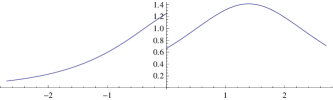
Figure 2. $\psi_{\omega,+}^{x_{1+},x_{2+}}$ for $\gamma=1$, $\lambda=1$, $\omega=9$ and pure soliton with $\omega=1$.

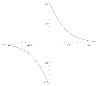
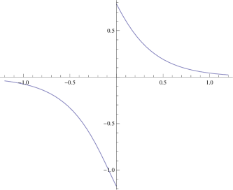
Figure 3. $\psi_{\omega,-}^{\bar{x},-\bar{x}}$ and $\psi_{\omega,-}^{x_{1+},x_{2+}}$ for $\gamma=1$, $\lambda=1$, $\omega=9.$

By direct comptutations, one can prove the following

Proposition 3.4.

The $L^{2}$-norm, the energy, and the action of the stationary states found in Theorem 3.3, are explicitly given by

1. For the unperturbed symmetric solitary wave

   $$\begin{split}\|\psi_{\omega,+}^{0,0}\|_{2}^{2}\ =\ \frac{4}{\lambda}\sqrt{\omega},\quad&\quad E_{\gamma\delta^{\prime}}(\psi_{\omega,+}^{0,0})\ =\ -\frac{2}{3\lambda}\omega^{\frac{3}{2}},\quad\quad S_{\omega}(\psi_{\omega,+}^{0,0})\ =\ \frac{4}{3\lambda}\omega^{\frac{3}{2}}.\\ \end{split}$$ (3.18)

2. For the asymmetric non-changing sign stationary states

   $$\begin{split}\|\psi_{\omega,+}^{x_{1\pm},x_{2\pm}}\|_{2}^{2}\ =&\ \frac{4}{\lambda}\sqrt{\omega}+\frac{2}{\lambda\gamma}\sqrt{1+\gamma^{2}\omega}-\frac{2}{\lambda\gamma}\\ E_{\gamma\delta^{\prime}}(\psi_{\omega,+}^{x_{1\pm},x_{2\pm}})\ =&\ -\frac{2}{3\lambda}\omega^{\frac{3}{2}}+\frac{2-\gamma^{2}\omega}{3\lambda\gamma^{3}}\sqrt{\gamma^{2}\omega+1}-\frac{2}{3\lambda\gamma^{3}}\\ S_{\omega}(\psi_{\omega,+}^{x_{1\pm},x_{2\pm}})\ =&\frac{4}{3\lambda}\omega^{\frac{3}{2}}+\frac{2}{3\lambda\gamma^{3}}(\gamma^{2}\omega+1)^{\frac{3}{2}}-\frac{\omega}{\lambda\gamma}-\frac{2}{3\lambda\gamma^{3}}\\ \end{split}$$ (3.19)

3. For the antisymmetric solutions

   $$\|\psi_{\omega,-}^{\bar{x},-\bar{x}}\|_{2}^{2}\ =\ \frac{4}{\lambda}\sqrt{\omega}-\frac{8}{\gamma\lambda},\quad E_{\gamma\delta^{\prime}}(\psi_{\omega,-}^{\bar{x},-\bar{x}})\ =\ \frac{16}{3\gamma^{3}\lambda}-\frac{2}{3\lambda}\omega^{\frac{3}{2}},\quad S_{\omega}(\psi_{\omega,-}^{\bar{x},-\bar{x}})\ =\ \frac{16}{3\gamma^{3}\lambda}-4\frac{\omega}{\gamma\lambda}+\frac{4}{3\lambda}\omega^{\frac{3}{2}}$$ (3.20)

4. For the asymmetric, changing sign solutions

   $$\begin{split}\|\psi_{\omega,-}^{\bar{x}_{1\pm},\bar{x}_{2\pm}}\|_{2}^{2}\ =&\ \frac{4}{\lambda}\sqrt{\omega}-\frac{2}{\lambda\gamma}\sqrt{1+\gamma^{2}\omega}-\frac{2}{\lambda\gamma}\\ E_{\gamma\delta^{\prime}}(\psi_{\omega,-}^{\bar{x}_{1\pm},\bar{x}_{2\pm}})\ =&\ -\frac{2}{3\lambda}\omega^{\frac{3}{2}}+\frac{\gamma^{2}\omega-2}{3\lambda\gamma^{3}}(\sqrt{\gamma^{2}\omega+1})-\frac{2}{3\lambda\gamma^{3}}\\ S_{\omega}(\psi_{\omega,-}^{\bar{x}_{1\pm},\bar{x}_{2\pm}})\ =&\frac{4}{3\lambda}\omega^{\frac{3}{2}}+\frac{2}{3\lambda\gamma^{3}}(\gamma^{2}\omega+1)^{\frac{3}{2}}-\frac{\omega}{\lambda\gamma}-\frac{2}{3\lambda\gamma^{3}}\\ \end{split}$$ (3.21)

Remark 3.5.

In any family of stationary states $\psi_{\omega,+}^{0,0}$, $\psi_{\omega,+}^{x_{1\pm},x_{2\pm}}$, $\psi_{\omega,-}^{\bar{x},-\bar{x}}$, and $\psi_{\omega,-}^{\bar{x}_{1\pm},\bar{x}_{2\pm}}$, introduced in Theorem 3.3, the $L^{2}$-norm is a monotonically increasing function of the frequency $\omega$ that diverges at infinity. In other words, it is a bijection of the interval $(0,+\infty)$ into itself.

3.3. Minimizing the action on the Nehari manifold

Here we consider the variational problem given by minimizing the action $S_{\omega}$ at fixed $\omega>0$ on the natural constraint called the Nehari manifold

$$E_{\gamma\delta^{\prime}}(\psi)-\frac{\lambda}{4}\|\psi\|_{4}^{4}\ =\ 0.$$ (3.22)

Proposition 3.6.

1. For any $\omega>0$,

$$S_{\omega}(\psi_{\omega,+}^{0,0})<S_{\omega}(\psi_{\omega,+}^{x_{1\pm},x_{2\pm}}).$$ (3.23)

2. For any $\omega>\frac{4}{\gamma^{2}}$,

$$S_{\omega}(\psi_{\omega,-}^{\bar{x},-\bar{x}})<S_{\omega}(\psi_{\omega,+}^{0,0})<S_{\omega}(\psi_{\omega,+}^{x_{1\pm},x_{2\pm}}).$$ (3.24)

3. For any $\omega>\frac{8}{\gamma^{2}}$,

$$S_{\omega}(\psi_{\omega,-}^{\bar{x}_{1\pm},\bar{x}_{2\pm}})<S_{\omega}(\psi_{\omega,-}^{\bar{x},-\bar{x}})<S_{\omega}(\psi_{\omega,+}^{0,0})<S_{\omega}(\psi_{\omega,+}^{x_{1\pm},x_{2\pm}}).$$ (3.25)

Proof.

Inequalities (3.23) and (3.24) follow immediately from (3.18), (3.19), (3.20).

The first inequality in (3.25) is proven by (3.20) and (3.21). In particular, one gets that the inequality is equivalent to

$$3\gamma^{2}\omega<6+\frac{2}{3}(\gamma^{2}\omega+1)^{\frac{3}{2}}$$

that is immediately verified for any $\omega>\frac{8}{\gamma^{2}}$. ∎

Remark 3.7.

Define the function $\Delta_{+}(\omega):=S_{\omega}(\psi_{\omega,+}^{x_{1,\pm},x_{2,\pm}})-S_{\omega}(\psi_{\omega,+}^{0,0})$ and remark that

$$\Delta_{+}(0)\ =\ \frac{d}{d\omega}\Delta_{+}(0)\ =\ 0,$$

while $\frac{d^{2}}{d\omega^{2}}\Delta_{+}(\omega)\ =\ \frac{\gamma^{2}}{2}(\gamma^{2}\omega+1)^{-1/2}\ >\ 0$.

This phenomenon suggests that the stationary states $\psi_{\omega,+}^{x_{1,\pm},x_{2,\pm}}$ bifurcate from a stationary state corresponding to the case with no defect, i.e., states of the type $\phi(\sqrt{\frac{2\omega}{\lambda}},\sqrt{\omega},x_{0})$, for some $x_{0}$, at $\omega>0$.

By an analogous computation one findes that the stationary states $\psi_{\omega,-}^{\bar{x}_{1\pm},\bar{x}_{2\pm}}$ bifurcate from $\psi_{\omega,-}^{\bar{x},-\bar{x}}$ at $\omega>\frac{8}{\gamma^{2}}$.

3.4. Minimizing the energy in the manifold of constant mass

Here we consider the variational problem of minimizing the energy $E_{\gamma\delta^{\prime}}$ on the manifold consisting of the function with given $L^{2}$-norm $\sqrt{\rho}>0$ and finite energy. As a consequence of Remark 3.5, one can parametrize the stationary states by the value $\rho$ of their squared $L^{2}$-norm $\rho\in(0,+\infty)$, instead of $\omega$. In the following, given $\rho>0$, we make use of the notation

$$\varphi_{\rho,+}^{0,0}\ :=\{\psi_{\omega,+}^{0,0},\ \omega\ \rm{s.t.}\ \|\psi_{\omega,+}^{0,0}\|_{2}^{2}\ =\ \rho\}$$

and analogously for the other families $\varphi_{\rho,+}^{x_{1\pm},x_{2\pm}}$, $\varphi_{\rho,-}^{\bar{x},-\bar{x}}$, and $\varphi_{\rho,-}^{\bar{x}_{1\pm},\bar{x}_{2\pm}}$.

Proposition 3.8.

1. For any $\rho>0$,

$$E_{\gamma\delta^{\prime}}(\varphi_{\rho,-}^{\bar{x},-\bar{x}})\ <\ E_{\gamma\delta^{\prime}}(\varphi_{\rho,+}^{0,0})\ <\ E_{\gamma\delta^{\prime}}(\varphi_{\rho,+}^{x_{1\pm},x_{2\pm}}).$$ (3.26)

2. For any $\rho>\frac{8}{\gamma\lambda}\left(\sqrt{2}-1\right)$,

$$E_{\gamma\delta^{\prime}}(\varphi_{\rho,-}^{\bar{x}_{1\pm},\bar{x}_{2\pm}})\ <\ E_{\gamma\delta^{\prime}}(\varphi_{\rho,-}^{\bar{x},-\bar{x}})\ <\ E_{\gamma\delta^{\prime}}(\varphi_{\rho,+}^{0,0})\ <\ E_{\gamma\delta^{\prime}}(\varphi_{\rho,+}^{x_{1\pm},x_{2\pm}}).$$ (3.27)

Proof.

In order to make the formulas less cumbersome, we show the computations for the particular case $\lambda=1$, $\gamma=1$ only. The general formulas can be then recovered by the scaling laws

$$\omega\to\gamma^{2}\omega,\quad\rho\to\gamma\lambda\rho,\quad E_{\delta^{\prime}}\to\gamma^{3}\lambda E_{\gamma\delta^{\prime}},$$ (3.28)

that can be directly verified.

Then, we make explicit the dependence of $\omega$, and then of the energy, on $\rho$. To this aim, it proves simpler and more practical to write down the function $\sqrt{\omega}(\rho)$ An elementary but lengthy computation shows that

• For the family $\varphi_{\rho,+}^{0,0}$

  $$\omega\ =\ \frac{\rho^{2}}{16},\qquad E_{\delta^{\prime}}(\varphi_{\rho,+}^{0,0})\ =\ -\frac{\rho^{3}}{96}.$$ (3.29)

• For the family $\varphi_{\rho,+}^{x_{1\pm},x_{2\pm}}$

  $$\begin{split}\sqrt{\omega}\ =&\ \frac{2\rho+4-\sqrt{\rho^{2}+4\rho+16}}{6}\\ \qquad E_{\delta^{\prime}}(\varphi_{\rho,+}^{x_{1\pm},x_{2\pm}})\ =&\ -\frac{5}{216}\rho^{3}+\frac{1}{54}(\rho^{2}+4\rho+16)^{\frac{3}{2}}-\frac{5}{36}\rho^{2}-\frac{4}{9}\rho-\frac{32}{27}.\end{split}$$ (3.30)

• For the family $\varphi_{\rho,-}^{\bar{x},-\bar{x}}$

  $$\sqrt{\omega}\ =\ \frac{\rho}{4}+2,\qquad E_{\delta^{\prime}}(\varphi_{\rho,-}^{-\bar{x},\bar{x}})\ =\ -\frac{\rho^{3}}{96}-\frac{\rho^{2}}{4}-2\rho.$$ (3.31)

• For the family $\varphi_{\rho,-}^{\bar{x}_{1\pm},\bar{x}_{2\pm}}$

  $$\begin{split}\sqrt{\omega}\ =&\ \frac{2\rho+4+\sqrt{\rho^{2}+4\rho+16}}{6}\\ \qquad E_{\delta^{\prime}}(\varphi_{\rho,-}^{\bar{x}_{1\pm},\bar{x}_{2\pm}})\ =&\ -\frac{5}{216}\rho^{3}-\frac{1}{54}(\rho^{2}+4\rho+16)^{\frac{3}{2}}-\frac{5}{36}\rho^{2}-\frac{4}{9}\rho-\frac{32}{27}.\end{split}$$ (3.32)

So, the first inequality in (3.26) is immediately proven. For the second inequality, one first extends by continuity the functions $E_{\delta^{\prime}}(\varphi_{\rho,+}^{0,0})$ and $E(\varphi_{\rho,+}^{x_{1\pm},x_{2\pm}})$ up to the value $\rho=0$ and obtains

$$\frac{d^{j}}{d\rho^{j}}E_{\delta^{\prime}}(\varphi_{0+,+}^{0,0})\ =\ \frac{d^{j}}{d\rho^{j}}E_{\delta^{\prime}}(\varphi_{0+,+}^{x_{1\pm},x_{2\pm}})\ =\ 0,\qquad j=0,1,2.$$

Furthermore,

$$\frac{d^{3}}{d\rho^{3}}E_{\delta^{\prime}}(\varphi_{0+,+}^{0,0})\ =\ \frac{d^{3}}{d\rho^{3}}E_{\delta^{\prime}}(\varphi_{0+,+}^{x_{1\pm},x_{2\pm}})\ =\ -\frac{1}{16}.$$

The second inequality in (3.26) is then proven by

$$0\ =\ \frac{d^{4}}{d\rho^{4}}E_{\delta^{\prime}}(\varphi_{\rho,+}^{0,0})\ <\ \frac{d^{4}}{d\rho^{4}}E_{\delta^{\prime}}(\varphi_{\rho,+}^{x_{1\pm},x_{2\pm}})\ =\ 12(\rho^{2}+4\rho+16)^{-\frac{5}{2}}.$$

It remains to prove the first inequality in (3.27). First, observe that

$$E_{\delta^{\prime}}(\varphi_{8(\sqrt{2}-1),-}^{\bar{x},-\bar{x}})\ =\ E_{\delta^{\prime}}(\varphi_{8(\sqrt{2}-1),-}^{\bar{x}_{1\pm},\bar{x}_{2\pm}})\ =\ -\frac{16}{3}(2\sqrt{2}-1)$$

and

$$\frac{d}{d\rho}E_{\delta^{\prime}}(\varphi_{8(\sqrt{2}-1),-}^{\bar{x},-\bar{x}})\ =\ \frac{d}{d\rho}E_{\delta^{\prime}}(\varphi_{8(\sqrt{2}-1),-}^{\bar{x}_{1\pm},\bar{x}_{2\pm}})\ =\ -4.$$

Now, we consider the second derivative. The statement $\frac{d^{2}}{d\rho^{2}}E_{\delta^{\prime}}(\varphi_{\rho,-}^{\bar{x},-\bar{x}})\ >\ \frac{d^{2}}{d\rho^{2}}E_{\delta^{\prime}}(\varphi_{\rho,-}^{\bar{x}_{1\pm},\bar{x}_{2\pm}})$ proves equivalent to $(\rho^{2}+4\rho^{\frac{1}{2}}+16)^{\frac{1}{2}}(\rho^{2}+4\rho^{\frac{1}{2}}+10)\ >\ -\frac{11}{16}\rho+\frac{2}{9}$, which is satisfied for any $\rho\geq 8(\sqrt{2}-1)$. The proof is complete.

∎

3.5. Linear limit for the stationary states

Theorem 3.9.

For $\lambda\to 0+$, the following limits hold:

$$\varphi_{\rho,+}^{0,0} \longrightarrow 0,\qquad{\mbox{in the weak topology of}}\,~{}Q_{\delta^{\prime}}$$ (3.33)

$$\varphi_{\rho,+}^{x_{1\pm},x_{2\pm}} \longrightarrow 0,\qquad{\mbox{in the weak topology of}}\,~{}Q_{\delta^{\prime}}$$ (3.34)

$$\varphi_{\rho,-}^{-\bar{x},\bar{x}} \longrightarrow \sqrt{\frac{2\rho}{\gamma}}e^{-\frac{2}{\gamma}|\cdot|},\qquad{\mbox{in the strong topology of}}\,~{}Q_{\delta^{\prime}}$$ (3.35)

Proof.

Limit (3.33) is immediately proven once observed that, afer rescaling (3.28), from (3.29) one has $\sqrt{\omega}=\frac{\lambda\rho}{4\sqrt{\gamma}},$ so that $\sqrt{\omega}$ vanishes in the limit.

To prove (3.34) notice that the first formula in (3.30), after rescaling (3.28), gives

$$\sqrt{\omega}\ =\ \frac{2\gamma\lambda\rho+4-\sqrt{\gamma^{2}\lambda^{2}\rho^{2}+4\gamma\lambda\rho+16}}{6\gamma},$$

so that $\sqrt{\omega}\approx\frac{\lambda\rho}{4\sqrt{\gamma}},$ as in the previous case.

Limit (3.35) is mapped into limit (2.5) by the replacement $\gamma\to\frac{4}{\alpha}$, so the reader is referred to the proof of Theorem 2.2.

∎

Remark 3.10.

Notice that the nonlinear limit for the stationary states $\varphi_{\rho,-}^{\bar{x}_{1\pm},\bar{x}_{2\pm}}$ is nonsensical: as $\lambda$ vanishes, the mass $\rho$ of the state is overcome by the threshold $\frac{8}{\lambda\gamma}(\sqrt{2}-1)$ under which there is no such a state. In other words, in order for $\varphi_{\rho,-}^{\bar{x}_{1\pm},\bar{x}_{2\pm}}$ to exist, the nonlinearity must be not only present, but also sufficiently strong.

Remark 3.11.

A closer look to the limit (3.34) shows that, in such case, both $x_{1+},x_{2+}$ diverge positively (analogously $x_{1-},x_{2-}$ diverge negatively) as $\lambda\to 0+$ (see (3.13), (3.3)). As a consequence, in the nonlinear limit the corresponding stationary state $\varphi_{\rho,+}^{x_{1\pm},x_{2\pm}}$ (or, equivalently, $\psi_{\omega,+}^{x_{1\pm},x_{2\pm}2}$) takes the shape of a soliton that runs towards the infinity. Conversely, this means that, starting from the linear dynamics generated by $H_{2}$ and turning on the nonlinearity, two stationary states arises from very far away and approach the origin as $\lambda$ grows.

Remark 3.12.

Limit (3.35) shows that the nonlinear symmetric changing sign stationary state $\varphi_{\rho,-}^{\bar{x},-\bar{x}}$ bifurcates from the linear ground state of the Hamiltonian $H_{2}$.

3.6. No-defect limits

As stressed in Section 1, we perform two kinds of no-defect limits.

Theorem 3.13.

For $\gamma\to 0+$, the following limits hold in the space $Q_{\delta^{\prime}}$ defined in (1.8):

$$\varphi_{\rho,+}^{x_{1\pm},x_{2\pm}} \longrightarrow \phi\left(\sqrt{\frac{\lambda}{2}}\frac{\rho}{2},\frac{\lambda\rho}{4},\frac{2}{\lambda\rho}\pm\log(3+2\sqrt{2})\right),~{}{\mbox{in the strong topology of}}\,~{}Q_{\delta^{\prime}}$$ (3.36)

$$\varphi_{\rho,-}^{-\bar{x},\bar{x}} \longrightarrow 0,\qquad{\mbox{in the sense of ditributions }}$$ (3.37)

Proof.

Limit (3.36) is obtained by observing that, by (3.30) with the rescaling (3.28), $\omega\approx\frac{\lambda\rho}{4}$ as $\lambda\to 0+$. As a consequence, by (3.3) and (3.12), one gets $x_{1\pm}\to\pm\frac{2}{\lambda\rho}\log(3+2\sqrt{2})$. (3.36) then follows from Lemma 1.1.

To prove (3.37) we just notice that, from the first identity in (3.31), $\omega\to\infty$ and, through (3.28), $\gamma\omega\to 2$. Then (3.15) shows that $\bar{x}\to\infty$. ∎

Remark 3.14.

It is immediate to observe that the stationary state $\varphi_{\rho,+}^{0,0}$ is untouched as $\gamma$ varies, while $\varphi_{\rho,-}^{\bar{x}_{1\pm},\bar{x}_{2\pm}}$ ceases to exist as $\gamma\leq\frac{8}{\lambda\rho}(\sqrt{2}-1)$.

Remark 3.15.

Limit (3.36) shows that the stationary states $\varphi_{\rho,+}^{x_{1\pm},x_{2\pm}}$ bifurcate from the nonlinear soliton $\phi\left(\sqrt{\frac{\lambda}{2}}\frac{\rho}{2},\frac{\lambda\rho}{4},\frac{2}{\lambda\rho}\log(3+2\sqrt{2})\right)$ at $\rho>0$.

Theorem 3.16.

For $\gamma\to+\infty$, the following limits hold in the space $Q_{\delta^{\prime}}$ defined in (1.8):

$$\varphi_{\rho,+}^{x_{1+},x_{2+}} \longrightarrow \chi_{(-\infty,0]}\,\phi\left(\sqrt{\frac{\lambda}{2}}\frac{\rho}{3},\frac{\lambda\rho}{6},0\right),\qquad{\mbox{in the weak topology of}}\,Q_{\delta^{\prime}}$$ (3.38)

$$\varphi_{\rho,-}^{-\bar{x},\bar{x}} \longrightarrow \phi\left(\sqrt{\frac{\lambda}{2}}\frac{\rho}{2},\frac{\lambda\rho}{4},0\right),\qquad{\mbox{in the strong topology of}}\,Q_{\delta^{\prime}}$$ (3.39)

$$\varphi_{\rho,-}^{\bar{x}_{1+},\bar{x}_{2+}} \longrightarrow \chi_{[0,+\infty)}\,\phi\left(\sqrt{\frac{\lambda}{2}}\rho,\frac{\lambda\rho}{2},0\right),\qquad{\mbox{in the strong topology of}}\,Q_{\delta^{\prime}}$$ (3.40)

where $\chi_{I}$ denotes the characteristic function of the set $I$.

Proof.

To prove the limit (3.38), notice first that, from (3.30) and the scaling law (3.28) one has $\sqrt{\omega}\to\frac{\lambda\rho}{6}$. Then, (3.3) shows that $t_{1}\to 0$ as $t_{2}\to 1$, so it must be $x_{1+}\to 0$ and $x_{2+}\to\infty$. Lemma (1.1) shows that in the left halfline the convergence is strong in the space $H^{1}({\mathbb{R}}^{-})$, while in the positive halfline there is a full soliton that run aways, weakening the convergence to zero.

Limit (3.39) is an immediate consequence of (3.31) and (3.15) through Lemma (1.1).

Finally, limit (3.40) is proven through (3.32), that shows $\sqrt{\omega}\to\frac{\rho}{2}$, (3.8), that gives $t_{1,+}\to 1$ and $t_{2,+}\to 0$, and Lemma (1.1). ∎

References

- [1] Adami R., Noja D.: Existence of dynamics for a 1-d NLS equation in dimension one, J. Phys. A, 42, 49, 495302, 19pp (2009).
- [2] Adami R., Noja D.: Stability and symmetry-breaking bifurcation for the Ground States of a NLS with a interaction, Commun. Math. Phys., 318, 247–289 (2013).
- [3] Adami R., Noja D., Visciglia N.: Constrained energy minimization and ground states for NLS with point defects, Disc. Cont. Dyn. Syst. B, 18, 5, 1155-1188 (2013).
- [4] Albeverio S., Brzeźniak Z., Dabrowski L.: Fundamental solutions of the Heat and Schrödinger Equations with point interaction, J. Func. An., 130, 220–254 (1995).
- [5] Albeverio S., Gesztesy F., Hoegh-Krohn R., Holden H.: Solvable Models in Quantum Mechanics, Springer-Verlag, New York (1988).
- [6] Albeverio S., Kurasov P.: Singular Perturbations of Differential Operators, Cambridge University Press 2000.
- [7] Cazenave T., Lions P.-L.: Orbital stability of standing waves for some nonlinear Schrödinger equations, Comm. Math. Phys., 85 549–561 (1982).
- [8] Cao Xiang D., Malomed A. B.: Soliton defect collisions in the nonlinear Schrödinger equation, Phys. Lett. A, 206, 177–182 (1995).
- [9] Cazenave, T.: Semilinear Schrödinger Equations, vol. 10 Courant Lecture Notes in Mathematics AMS, Providence (2003).
- [10] Fukuizumi R., Jeanjean L.: Stability of standing waves for a nonlinear Schrödinger equation with a repulsive Dirac delta potential, Dis. Cont. Dyn. Syst. (A), 21, 129–144 (2008).
- [11] Fukuizumi R., Ohta M, Ozawa T.: Nonlinear Schrödinger equation with a point defect, Ann. Inst. H. Poincaré - AN, 25, 837–845 (2008).
- [12] Fukuizumi R., Sacchetti A.: Bifurcation and stability for nonlinear Schrödinger equation with double well potential in the semiclassical limit, arxiv:1104.1511v1, to appear on J. Stat. Phys. (2011).
- [13] Goodman R. H., Holmes P. J., Weinstein M.I.: Strong NLS soliton-defect interactions, Physica D, 192, 215–248 (2004).
- [14] Le Coz S., Fukuizumi R., Fibich G., Ksherim B., Sivan Y.: Instability of bound states of a nonlinear Schr dinger equation with a Dirac potential, Phys. D, 237 n. 8, 1103–1128 (2008).
- [15] Witthaut D., Mossmann S., Korsch H. J.: Bound and resonance states of the nonlinear Schrödinger equation in simple model systems, J. Phys. A, 38, 1777-1702 (2005).
- [16] Zakharov V.E., Shabat A.B.: A scheme for integrating the nonlinear equations of mathematical physics by the method of the inverse scattering problem. I. Funct. Anal. Appl., 8, 226 235, (1974).