Stable and flexible system for glucose homeostasis

Abstract

Pancreatic islets, controlling glucose homeostasis, consist of $\alpha$, $\beta$, and $\delta$ cells. It has been observed that $\alpha$ and $\beta$ cells generate out-of-phase synchronization in the release of glucagon and insulin, counter-regulatory hormones for increasing and decreasing glucose levels, while $\beta$ and $\delta$ cells produce in-phase synchronization in the release of the insulin and somatostatin. Pieces of interactions between the islet cells have been observed for a long time, although their physiological role as a whole has not been explored yet. We model the synchronized hormone pulses of islets with coupled phase oscillators that incorporate the observed cellular interactions. The integrated model shows that the interaction from $\beta$ to $\delta$ cells, of which sign has controversial reports, should be positive to reproduce the in-phase synchronization between $\beta$ and $\delta$ cells. The model also suggests that $\delta$ cells help the islet system flexibly respond to changes of glucose environment.

I Introduction

Life maintain energy through metabolism. Among the two major fuels of our body, glucose and lipid, glucose is the primary energy source, particularly for brain cells. Therefore, maintaining glucose levels constant, glucose homeostasis, is essential for life. Its failure leads to a metabolic disease, diabetes. Islets of Langerhans in the pancreas play a critical role for maintaing the glucose homeostasis. It is composed of three major cell types: $\alpha$, $\beta$, and $\delta$ cells. During fasting and fed states, $\alpha$ and $\beta$ cells secrete glucagon and insulin, respectively, for increasing and decreasing glucose levels. At first sight, these two reciprocal cells seem sufficient for controlling glucose levels. However, a third one, $\delta$ cell, has been found, and its role on the glucose homeostasis has yet to be unveiled.

Like other hormones in the body, the insulin and glucagon secretions show rhythmic behavior ref:Lefebvre . Their oscillation with $5-10$ minute periods have been repeatedly observed not only in the cells within islets ref:Bergsten , but also in isolated cells ref:Grapengiesser . In particular, the periodic insulin release has been extensively studied with mathematical modeling ref:Bertram . It has been reported that glucagon and insulin exhibit out-of-phase synchronization both in vivo ref:Menge and in vitro ref:Hellman . The in vitro study ref:Hellman has also shown that insulin and somatostatin (secreted by $\delta$ cells) have in-phase synchronization. In addition, Menge et al demonstrated that the out-of-phase synchronization is disrupted in diabetes patients, suggesting the physiological importance of the coordinated insulin and glucagon secretion ref:Menge . It has long been observed that the endocrine cells interact with each other through hormones and/or neurotransmitters ref:Koh .

Synchronization between coupled oscillators has long been studied in physics ref:synch . In particular, the Kuramoto model has been introduced to explain collective behavior such as synchronization in the population of coupled oscillators ref:Kuramoto , and recently generalized by allowing the coupling with arbitrary phase shift  ref:Pikovsky_Rosenblum . In other words, the general model can have arbitrary signs and strengths of coupling, while the original model has only positive coupling. Hong and Strogatz have proposed an interesting specification of the generalized Kuramoto model in which two populations of conformists (having positive coupling) and contrarians (negative coupling) interact and show rich dynamics ref:Hong_Strogatz_PRL . As a natural extension, the synchronization between three symmetrically-distinct populations is of particular interest. Here we introduce a perfect realization of the three-body interaction in biology.

Using the generalized Kuramoto model, we specifically answer the following question: Are the observed pieces of local interactions between $\alpha$, $\beta$, and $\delta$ cells sufficient and consistent to explain the synchronized hormone secretion? We also explore the role of the third population, $\delta$ cells, additional to the counter-regulating $\alpha$ and $\beta$ cells in the control system for homeostasis.

This paper consists of five sections. In Sec. II, synchronized hormone pulses of $\alpha$, $\beta$, and $\delta$ cells are described by the three coupled phase oscillators. Section III derives a generalized islet model that considers population of each cell type. Section IV presents results and predictions of the islet model. Finally, Sec. V summarizes and discusses the results.

II Islet model

To understand the synchronized hormone pulses in the pancreatic islets, we simply regard the endocrine cells as intrinsic oscillators producing pulsatile hormones because isolated cells still show oscillations in the absence of neighboring cells. Then, the attractive or repulsive interaction between the oscillators play a role to synchronize them in phase or out of phase. Since we are interested in only the phases of the three interacting oscillators of $\alpha$, $\beta$, and $\delta$ cells, their synchronization dynamics can be described by three coupled oscillators with Kuramoto-type interactions ref:Kuramoto :

$$\dot{\theta}_{1} = \omega_{1}+J_{21}\sin(\theta_{2}-\theta_{1})+J_{31}\sin(\theta_{3}-\theta_{1}),$$ (1)

$$\dot{\theta}_{2} = \omega_{2}+J_{12}\sin(\theta_{1}-\theta_{2})+J_{32}\sin(\theta_{3}-\theta_{2}),$$ (2)

$$\dot{\theta}_{3} = \omega_{3}+J_{13}\sin(\theta_{1}-\theta_{3})+J_{23}\sin(\theta_{2}-\theta_{3}).$$ (3)

The subscripts 1, 2, and 3 here correspond to $\alpha$, $\beta$, and $\delta$ cells, respectively.

The variable $\omega_{1,2,3}$ denotes their natural frequencies. $J_{s^{\prime}s}$ represents the coupling (interaction) strength from the $s^{\prime}$ cell onto the $s$ cell (Fig. 1). The sign of the couplings $J_{s^{\prime}s}$ between $\alpha$, $\beta$, and $\delta$ cells can be found in the literatures and is summarized in the Table 1. We consider here the case of asymmetric couplings ($J_{s^{\prime}s}\neq J_{ss^{\prime}}$), and further include repulsive interaction with negative strength ($J_{s^{\prime}s}<0$) in addition to the attractive one with positive value ($J_{s^{\prime}s}>0$). The repulsive and attractive coupling has also been known to appear in the neural networks with excitatory and inhibitory coupling ref:excitatory_inhibitory , where the positive coupling is for the excitatory neurons, and the negative one for the inhibitory neurons, respectively. To facilitate the comparison with the recent reports ref:Hellman , we suppose that $J_{12}=J_{13}=p~{}(>0)$, $-J_{21}=J_{23}=q~{}(>0)$, and $-J_{31}=-J_{32}=r~{}(>0)$ for the interactions between cell types. It is reasonable to assume that the interaction strengths from the $s$ cell to the $s^{\prime}$ and $s^{\prime\prime}$ cell are equivalent as $|J_{ss^{\prime}}|=|J_{ss^{\prime\prime}}|$, because the interactions are realized by the same molecules secreted from the $s$ cell.

To simplify our system, and in reasonable agreement with observations ref:Grapengiesser , we assume that the oscillators in Eq. (6) have the same natural frequency ($\omega_{1,2,3}=\omega$). Then, since we are interested in the phase differences between cell types, Eq. (1) is then reduced to

$$\dot{u} = (q-p)\sin u+r\big{[}\sin v+\sin(u-v)\big{]},$$ (4)

$$\dot{v} = q\big{[}\sin u+\sin(u-v)\big{]}+(r-p)\sin v,$$ (5)

where $u\equiv\theta_{1}-\theta_{2}$ and $v\equiv\theta_{1}-\theta_{3}$.

In the following section, we derive a generalized islet model considering populations of each cell type in the islet. However, because the population model results in essentially the same conclusion, readers who are not interested in the sophisticated analysis may skip Sec III.

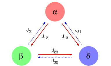
Figure 1: (Color online) Schematic diagram of $\alpha$, $\beta$, and $\delta$ cells in the pancreatic islets. The red (solid) arrows represent the attractive interaction from the $s$ cell to the $s^{\prime}$ cell, with the positive strength $(J_{ss^{\prime}}>0)$, and the blue (dotted) arrows denote the repulsive interaction, with the negative strength $(J_{ss^{\prime}}<0)$, respectively. The sign of cellular interactions has been taken from the known facts based on the observations (see the Table 1).

Parameter	Interaction	Sign	Reference
$J_{12}$	$\alpha\rightarrow\beta$	$+$	ref:J12
$J_{13}$	$\alpha\rightarrow\delta$	$+$	ref:J13
$J_{21}$	$\beta\rightarrow\alpha$	$-$	ref:J21
$J_{23}$	$\beta\rightarrow\delta$	$+$	ref:J23a
		$0$	ref:J23b
$J_{31}$	$\delta\rightarrow\alpha$	$-$	ref:J31J32
$J_{32}$	$\delta\rightarrow\beta$	$-$	ref:J31J32

Table 1: Signs of cellular interactions in literatures.

III Population model

Considering populations of each cell type, we develop a model of coupled phase oscillators for the cells in the islet which is governed by

$$\dot{\phi}^{s}_{j}=\omega^{s}_{j}+\frac{1}{N}\sum_{s^{\prime}=1}^{3}\sum_{k=1}^{N_{s^{\prime}}}J_{{s^{\prime}}s}\sin(\phi^{s^{\prime}}_{k}-\phi^{s}_{j})$$ (6)

for $s=1,2,3$, where $j=1,\cdots,N_{s}$, and $\phi^{s}_{j}$ represents the phase/angle of the oscillator $j$ in subpopulation $s$. The number $N_{s}$ is the size of the subpopulation $s$: $N=\sum_{s=1}^{3}N_{s}$. The subpopulation with $s=1,2,3$ here corresponds to the subgroup that consists of $\alpha$, $\beta$, and $\delta$ cells, respectively. The variable $\omega^{s}_{j}$ denotes the natural frequency of the oscillator $j$ in the subpopulation $s$, where we assumed that the oscillators have the same natural frequency ($\omega^{s}_{j}=\omega$). $J_{s^{\prime}s}$ represents the coupling (interaction) strength from the oscillators in the subpopulation $s^{\prime}$ onto those in the subpopulation $s$. We note that a model similar to Eq. (6) has been introduced in previous studies ref:Daniel_Steve ; ref:Pikovsky_Rosenblum .

Here we can set $\omega$ to zero without loss of generality by the phase transformation: $\phi^{s}_{j}\rightarrow\phi^{s}_{j}+\omega t$. Eq. (6) is then rewritten as

$$\dot{\phi}^{s}_{j}=g_{s}e^{i\phi^{s}_{j}}+{\bar{g}_{s}}e^{-i\phi^{s}_{j}},$$ (7)

where $g_{s}=\frac{i}{2N}\sum_{s^{\prime}=1}^{3}\sum_{k=1}^{N_{s^{\prime}}}J_{s^{\prime}s}e^{-i\phi^{s^{\prime}}_{k}}$ and $\bar{g}_{s}$ is its complex conjugate.

Collective synchronization in the system of coupled oscillators is conveniently measured by the complex order parameter ref:Kuramoto ; ref:synch

$$Z\equiv Re^{i\Theta}=\frac{1}{N}\sum_{k=1}^{N}e^{i\phi_{k}},$$ (8)

where $R$ is a global order parameter that measures the phase coherence over all oscillators for the whole system, and $\Theta$ is the average phase. This order parameter $Z$ can be divided into three terms:

$$Z(t)=n_{1}z_{1}+n_{2}z_{2}+n_{3}z_{3}$$ (9)

with $n_{s}=N_{s}/N$ and $z_{s}=(1/N_{s})\sum_{k=1}^{N_{s}}e^{i\phi^{s}_{k}}$, where $z_{s}$ represents a local order parameter for the subpopulation $s~{}(=1,2,3)$.

We now consider the continuum limit, $N\rightarrow\infty$. In this limit, the order parameter $Z(t)$ can be written as

$$Z(t)=\int_{0}^{2\pi}e^{i\phi}f(\phi,t)d\phi,$$ (10)

where $f(\phi,t)$ denotes the probability density function of the phases that lie between $\phi$ and $\phi+d\phi$ at time $t$. Following the Ott-Antonsen ansatz ref:OA , we let

$$f(\phi,t)=\frac{1}{2\pi}\Bigg{\{}1+\sum_{n=1}^{\infty}\big{[}\bar{\alpha}(t)^{n}e^{in\phi}+\alpha(t)^{n}e^{-in\phi}\big{]}\Bigg{\}}$$ (11)

for some unknown function $\alpha$ that is independent of $\phi$. We note that Eq. (11) is equivalent to the usual form of the Poisson kernel ref:Mobius_transformation

$$f(\phi)=\frac{1}{2\pi}\frac{1-\rho^{2}}{1-2\rho\cos(\phi-\theta)+\rho^{2}},$$ (12)

where $\rho$ and $\theta$ are defined via $\alpha=\rho e^{i\theta}$, and $\sum_{n=1}^{\infty}\bar{\alpha}^{n}e^{in\phi}=\bar{\alpha}e^{i\phi}/(1-\bar{\alpha}e^{i\phi})$ is used. With this, we find that $\alpha(t)$ in Eq. (11) can be interpreted as the order parameter $Z(t)$, where $\rho$ and $\theta$ correspond to $R$ and $\Theta$ in Eq. (8), respectively. On the Poisson submanifold that is expressed by Eq. (11) each probability density function $f_{s}$ for the subpopulation $s$ is also a Poisson kernel, therefore it has the same Fourier expansion as Eq. (11), with $\alpha_{s}$ instead of $\alpha$: $f_{s}=\frac{1}{2\pi}\{1+\sum_{n=1}^{\infty}[\bar{\alpha}_{s}(t)^{n}e^{in\phi}+\alpha_{s}(t)^{n}e^{-in\phi}]\}$. Here, $\alpha_{s}$ corresponds to the local order parameter for the subpopulation $s$: $\alpha_{s}=\rho_{s}e^{i\theta_{s}}=z_{s}$. Substituting Eq. (11) into Eq. (10), we find $Z(t)=\alpha(t)$, which further yields $Z(t)=\sum_{s=1}^{3}n_{s}\alpha_{s}(t)$.

Meanwhile, we expect that the continuity equation is satisfied for each subpopulation as

$$\frac{\partial f_{s}}{\partial t}+\frac{\partial}{\partial\phi}(f_{s}v_{s})=0,$$ (13)

where $f_{s}$ is the probability density function for the subpopulation $s$, and $v_{s}$ is the velocity field given by $v_{s}(\phi,t)=g_{s}e^{i\phi}+\bar{g_{s}}e^{-i\phi}$. Substituting $f_{s}$ and $v_{s}$ into Eq. (13), we obtain

$$\big{[}\dot{\alpha}_{s}-i(g_{s}\alpha^{2}_{s}+\bar{g}_{s})\big{]}\sum_{n=1}^{\infty}n{\alpha_{s}}^{n-1}e^{-in\phi}+c.c=0,$$ (14)

where $c.c$ denotes the complex conjugate of the first term. We find that the summation in Eq. (14) does not vanish, thus the factor in front of the summation should be zero, which leads to

$$\dot{\alpha}_{s}=i(g_{s}\alpha^{2}_{s}+\bar{g}_{s}).$$ (15)

This means that $z_{s}(t)$ also evolves according to $\dot{z}_{s}=i(g_{s}z^{2}_{s}+\bar{g}_{s})$.

We supposed that $J_{12}=J_{13}=p~{}(>0)$, $-J_{21}=J_{23}=q~{}(>0)$, and $-J_{31}=-J_{32}=r~{}(>0)$ for the interactions between the subpopulations. For the subpopulation self-coupling, on the other hand, we let $J_{11}=I_{1}$, $J_{22}=I_{2}$, and $J_{33}=I_{3}$, where $I_{1},I_{2},I_{3}$ are all larger than $p,q,r$, which means that the coupling strength within a group is stronger than that between the subpopulations. With these interactions, and with the substitution of $\alpha_{s}=\rho_{s}e^{i\theta_{s}}$ into Eq. (15) for $s=1,2,3$, we find that the dynamics of each subpopulation is governed by

$$\dot{\rho_{1}} = \frac{1\!-\!\rho_{1}^{2}}{2}\big{[}I_{1}n_{1}\rho_{1}-qn_{2}\rho_{2}\cos u-rn_{3}\rho_{3}\cos v\big{]},$$

$$\dot{\theta_{1}} = \frac{1\!+\!\rho_{1}^{2}}{2\rho_{1}}\big{[}qn_{2}\rho_{2}\sin u+rn_{3}\rho_{3}\sin v\big{]},$$ (16)

$$\dot{\rho_{2}} = \frac{1\!-\!\rho_{2}^{2}}{2}\big{[}pn_{1}\rho_{1}\cos u+I_{2}n_{2}\rho_{2}-rn_{3}\rho_{3}\cos(u-v)\big{]},$$

$$\dot{\theta_{2}} = \frac{1\!+\!\rho_{2}^{2}}{2\rho_{2}}\big{[}pn_{1}\rho_{1}\sin u-rn_{3}\rho_{3}\sin(u-v)\big{]},$$ (17)

$$\dot{\rho_{3}} = \frac{1\!-\!\rho_{3}^{2}}{2}\big{[}pn_{1}\rho_{1}\cos v+qn_{2}\rho_{2}\cos(u-v)+I_{3}n_{3}\rho_{3}\big{]},$$

$$\dot{\theta_{3}} = \frac{1\!+\!\rho_{3}^{2}}{2\rho_{3}}\big{[}pn_{1}\rho_{1}\sin v-qn_{2}\rho_{2}\sin(u-v)\big{]},$$ (18)

respectively, where $u\equiv\theta_{1}-\theta_{2}$, and $v\equiv\theta_{1}-\theta_{3}$. For one simple case, we can assume that each subpopulation is in perfect synchronization ($\rho_{1}=\rho_{2}=\rho_{3}=1$). We note that this assumption is consistent with the experimental observation that $\beta$ cells, sharing gap-junction channels with adjacent $\beta$ cells, are strongly synchronized ($\rho_{2}=1$) ref:Ravier . The long-range interaction between remote $\beta$ cells has been mechanically justified by showing that the gap junctions mediate calcium waves in islets  ref:Benninger . On the other hand, no clear evidence for self-synchronization of $\alpha$ and $\delta$ cells has been found. However, pulsatile glucagon and somatostatin secretions of $\alpha$ and $\delta$ cells imply their self-synchronization ($\rho_{1}=1$ and $\rho_{3}=1$). Otherwise, asynchronous hormone pulses would compensate each other, and their averaged pulses would become flat. Then, since we are interested in the phase differences between cell types, Eq. (III)-(III) is then reduced to

$$\dot{u} = (qn_{2}-pn_{1})\sin u+rn_{3}\big{[}\sin v+\sin(u-v)\big{]},$$ (19)

$$\dot{v} = qn_{2}\big{[}\sin u+\sin(u-v)\big{]}+(rn_{3}-pn_{1})\sin v.$$ (20)

Therefore, we arrived at the same conclusion in Eq. (4)-(5), except for weighting population densities to the coupling strengths ($p\rightarrow pn_{1}$, $q\rightarrow qn_{2}$, and $r\rightarrow rn_{3}$).

IV Model analysis

We now examine the synchronization patterns of the islet model in Eq. (4)-(5). Specifically, we pay attention to the fixed point $(u^{*},v^{*})$ that is obtained from $\dot{u}=0$ and $\dot{v}=0$. It is found that $(0,0)$, $(0,\pm\pi)$, $(\pm\pi,0)$, and $(\pm\pi,\pm\pi)$ are all fixed points of Eq. (4) and (5). Note that some parameter set ($p$, $q$, $r$) allows nontrivial fixed points ($u_{\pm}$, $v_{\pm}$), satisfying $\tan u_{\pm}=\mp pqh/r(h^{2}-2pq)$ and $\tan v_{\pm}=\pm(p-q+r)h/(h^{2}-2pr)$ with $h=\sqrt{2pq+2qr+2rp-p^{2}-q^{2}-r^{2}}$. The stability of the fixed points has been checked, using the linear stability analysis footnote1 .

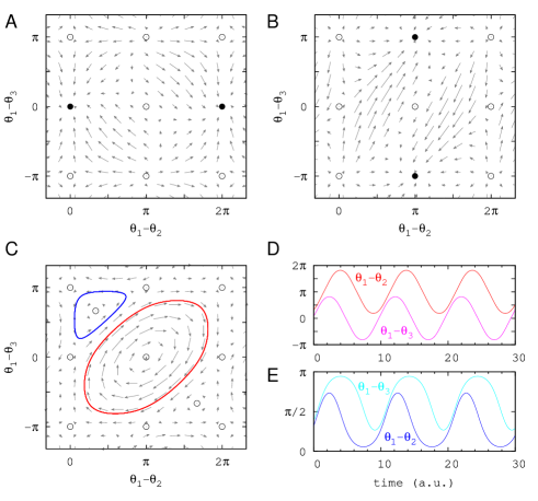
Figure 2: (Color online) Vector flow (A) for the state $(0,0)$ for $p>q+r$; (B) the state $(\pi,\pi)$ for $q>p+r$; and (C) traveling wave (limit-cycle) for $p=q=r$. Note that filled/empty circles represent stable/unstable fixed points. The temporal evolution of $u(t)=\theta_{1}(t)-\theta_{2}(t)$ and $v(t)=\theta_{1}(t)-\theta_{3}(t)$ for the (D) red (clockwise limit cycle) and (E) blue (counter-clockwise limit cycle) regions in (C).

We find that the stability of the fixed point depends on the parameter values of $p$, $q$, and $r$: When the interaction by $\alpha$ cells is dominant ($p>q+r$) at fasting conditions with low glucose levels, the system approaches the stable fixed point $(0,0)$, showing an in-phase synchrony for $\alpha$-$\beta$, $\alpha$-$\delta$, and $\beta$-$\delta$ (Fig.  2A).

On the other hand, when the interaction by $\beta$ cells is dominant ($q>p+r$) at fed conditions with high glucose levels, the system approaches the stable fixed point $(\pi,\pi)$, showing an out-of-phase synchrony for both $\alpha$-$\beta$ and $\alpha$-$\delta$, while an in-phase synchrony for $\beta$-$\delta$ (Fig. 2B). Note that when we additionally consider population densities, the inequality ($q>p+r$) becomes $qn_{2}>pn_{1}+rn_{3}$. Because most cells in the pancreatic islets are $\beta$ cells ($n_{2}>n_{1}>n_{3}$), we naturally expect that the population dominance of $\beta$ cells is more likely to lead the islet system to the $(\pi,\pi)$ state.

At near normal glucose conditions when the dominance of $\alpha$ and $\beta$ cell interactions is relaxed (e.g., $p=q=r$), present is a new stationary solution of limit cycles with $\dot{u}\neq 0$ and $\dot{v}\neq 0$. The limit cycles in the ($u$, $v$) plane (see Fig. 2C), oscillate between the ($0$, $0$) and ($\pi$, $\pi$) states (see Figs. 2D and E). We summarized these dynamic behaviors depending on relative coupling strengths in the phase diagram of Fig. 3.

What happens if $\delta$ cells are absent? Biologically, this is a very important question since it may give some clue about the very reason why $\delta$ cells are found in pancreatic islets. According to our model, when $\delta$ cells are absent, Eq. (III) and (III) are reduced to

$$\dot{u}=(q-p)\sin u.$$ (21)

We find that $u=\pi$ is the stable fixed point for $q>p$, on the other hand $u=0$ is the stable fixed point for $p>q$. Note that for $p=q$, traveling wave (TW) states exist with $u\neq 0$ or $\pi$, but $\dot{u}=0$. This TW state has been reported in Ref. ref:Hong_Strogatz_PRL ; it is known to be induced by the asymmetry in the coupling parameters. In the islet system, the coupling is also asymmetric one $(J_{s^{\prime}s}\neq J_{ss^{\prime}})$, accordingly a TW state is naturally expected to appear. This implies that the change from one state (out-of-phase synchrony between the $\alpha$ and $\beta$ cells) to another one (in-phase synchrony between the cells) occurs drastically depending on the range of interaction strength. In the absence of $\delta$ cells, the drastic state change can be easily seen in the phase diagram ($r=0$) of Fig. 3. Note that this is very awkward situation where small perturbations of glucose (influencing relative strengths of $p$ and $q$) can result in completely different states of islets. In contrast, in the presence of $\delta$ cells, islets allow flexible changes between $u=0$ and $u=\pi$ states using limit cycles as shown for $r\neq 0$ in Fig. 3.

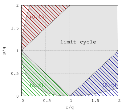
Figure 3: (Color online) Phase diagram for relative strengths of $p$, $q$, and $r$. Stable fixed points ($\theta_{1}-\theta_{2}$, $\theta_{1}-\theta_{3}$)=(0, 0) for $p>q+r$ (red hatched area); ($\pi$, $\pi$) for $q>p+r$ (green hatched area); (0, $\pi$) for $r>p+q$ (blue hatched area); and limit cycles for $2pq+2pr+2qr-p^{2}-q^{2}-r^{2}>0$ (gray area). Some regions have both fixed points and limit cycles as solutions depending on initial conditions.

V Discussion

In summary, we developed a model of coupled phase oscillators for the cells in pancreatic islets that explains their synchronized hormone pulses. The model provides a clear picture about the characteristics of the cell-cell interactions in the islet, and suggests an important role of the third population, $\delta$ cells.

In this paper, the islet system provides a natural extension of the Kuramoto model. In the original model, every oscillator has the same positive coupling between them ref:Kuramoto . Next simplest possible scenario may be to consider interactions between two distinct populations in which one population (conformists) has positive coupling, while the other one (contrarians) has negative coupling. This system has been demonstrated to show rich dynamics such as out-of-phase synchrony between conformists and contrarians, and traveling wave states where the phase difference between two populations is fixed, but each population still oscillates with a new frequency different from their mean natural frequency ref:Hong_Strogatz_PRL . Our study introduces a third population that is symmetrically distinct from the conformists and contrarians. The third one should have a mixed coupling with positive and negative signs depending on neighbors. The three-population model has larger flexibility in synchronization than the two-population model as expected. In addition to the in-phase and out-of-phase synchrony solutions, the limit cycle solutions allow three populations have periodic phase changes between them.

The islet system is an interesting realization of the three-population model. Furthermore, the simple model of phase oscillators allows to understand biological meanings of symmetries of cellular interactions and functional roles of each population. One main outcome of our model is the enlightenment of the sign of the $\beta\rightarrow\delta$ interaction, $J_{23}$. So far, consistency on the sign of interactions between $\alpha$, $\beta$, and $\delta$ cells has been observed, except for the $J_{23}$ (see Table 1). It has been reported that the interaction is positive in chicken pancreas ref:J23a , while other studies in canine (dog) pancreas reported it as negligible ref:J23b . Although we can not exclude species differences, the technical difficulty of measuring the infinitesimal amount of somatostatin ($\sim$femtomole), may explain the inconsistency. It has been reported that birds have surprisingly abundant $\delta$ cells in the islets, compared with mammal islets (40% vs. 10%) ref:Hara . The extreme excess of $\delta$ cells in chicken might allow to detect the stimulating effect of insulin secreted by $\beta$ cells. In our model, we have found that if $J_{23}\leq 0$, it is impossible to generate the reported in-phase synchronization between $\beta$ and $\delta$ cells. The positive interaction breaks the symmetry between $\beta$ and $\delta$ cells, and gives three symmetrically-distinguishable cell populations (Fig. 1): $\alpha$ cells activate other populations; $\delta$ cells suppress other populations; while $\beta$ cells stimulate and suppress other populations. In other words, $\alpha$ cells are only suppressed by other populations; $\delta$ cells are only activated by other populations; while $\beta$ cells are both activated and suppressed by other populations. It is of interest that evolutionary lower species have only two reciprocal partners of $\alpha$ and $\beta$ cells, while higher species are equipped with symmetrically different three cell populations ref:Hara .

In addition to the conjecture of $J_{23}>0$, we found a potential role of the third population, $\delta$ cells. Regardless of the existence of $\delta$ cells, the islet model with an asymmetric interaction between $\alpha$ and $\beta$ cells produces both out-of-phase and in-phase hormone pulses of $\alpha$ and $\beta$ cells depending on the dominance of the inhibitory (repulsive) interaction ($\beta\rightarrow\alpha$) and the excitatory (attractive) interaction ($\alpha\rightarrow\beta$). The different synchronization patterns may be beneficial for controlling glucose levels. Under high glucose conditions, insulin plays a role to decrease glucose levels. Continuous action of excess insulin can cause episodes of hypoglycemia (diminished glucose in blood), which is more dangerous than hyperglycemia (excessive glucose in blood) because it results in shock and finally death. Therefore, intermittent glucagon pulses at the high glucose conditions can prevent to enter into hypoglycemia. If the glucagon pulses were in phase with insulin pulses, their actions in the liver, increasing and decreasing blood glucose levels, would compete, resulting in inefficient glucose control. On the other hand, under low glucose conditions, insulin secretion becomes negligible, remaining just at a basal insulin level, and glucagon plays a role to increase glucose levels. The basal insulin helps cells in the body to absorb available glucose. Therefore, at the low glucose conditions, the in-phase glucagon and insulin pulses can be beneficial, because insulin accelerates the immediate absorption of glucose produced by glucagon. Indeed the out-of-phase state in a postprandial condition has been observed ref:Menge , and the in-phase state after an overnight fast has also been reported ref:Lang . Then, one may wonder which states the islet takes at normal glucose levels. While the absence of $\delta$ cells allows only the two states of in-phase and out-of-phase, the presence of $\delta$ cells generates an oscillating state between the two.We suggest that this oscillation maximizes the flexibility of the islet system to quickly respond to uncertain glucose inputs. This last point is left for further study.

Finally, note that our simple phenomenological model is limited to explain the physiological rationale for hormone pulsatility, although it has been proposed that the periodic exposure to the hormones can prevent desensitization of their receptors, compared with their continuous exposure ref:Hellman_review .

We thank Jean-Emile Bourgine for a critical reading of the manuscript. This research was supported by Basic Science Research funded by NRF No. 2012R1A1A2003678 (H.H.), by Ministry of Science, ICT & Future Planning No. 2013R1A1A1006655 (J.J), and by the Max Planck Society, the Korea Ministry of Education, Science and Technology, Gyeongsangbuk-Do and Pohang City (J.J).

References

- (1) P.J. Lefébvre, G. Paolisso, A.J. Scheen, and J.C. Henquin, Diabetologia 30, 443 (1987).
- (2) P. Bergsten, E. Grapengiesser, E. Gylfe, A. Tengholm, and B. Hellman, J. Biol. Chem. 269, 8749 (1994).
- (3) E. Grapengiesser, E. Gylfe, and B. Hellman, J. Biol. Chem. 266, 12207 (1991); M.A. Ravier and G.A. Rutter, Diabetes 54, 1789 (2005).
- (4) R. Bertram, A. Sherman, and L.S. Satin, Am. J. Physiol. Endocrinol. Metab. 293, E890 (2007).
- (5) B.A. Menge et al., Diabetes 60, 2160 (2011).
- (6) B. Hellman, A. Salehi, E. Gylfe, H. Dansk, and E. Grapengiesser, Endocrinology 150, 5334 (2009); B. Hellman, A. Salehi, E. Grapengiesser, and E. Gylfe, Biochem. Biophys. Res. Commun. 417 1219 (2012).
- (7) D.S. Koh, J.H. Cho, and L. Chen, J. Mol. Neurosci. 48, 429 (2012).
- (8) A.T. Winfree, The Geometry of Biological Time (Springer, New York, 1980); A. Pikovsky, M. Rosenblum, and J. Kurths, Synchronization (Cambridge University Press, Cambridge, 2001); S.H. Strogatz, Sync (Hyperion, New York, 2003); J. A. Acebron et al., Rev. Mod. Phys. 77, 137 (2005).
- (9) Y. Kuramoto, Chemical Oscillations, Waves, and Turbulence (Springer, Berlin, 1984).
- (10) A. Pikovsky and M. Rosenblum, Phys. Rev. Lett. 101, 264103 (2008).
- (11) H. Hong and S. H. Strogatz, Phys. Rev. Lett. 106, 054102 (2011).
- (12) E. Samols, G. Marri, and V. Marks, Lancet 2, 415 (1965); K. Kawai et al., Diabetologia 38, 274 (1995); H. Brereton, M.J. Carvell, S.J. Persaud, and P.M. Jones, Endocrine 31, 61 (2007).
- (13) G.S. Patton, R. Dobbs, L. Orci, W. Vale, and R.H. Unger, Metabolism 25, 1499 (1976); G.C. Weir, E. Samols, J.A. Day, and Y.C. Patel, Metabolism 27, 1223 (1978); J. Dolais-Kitabgi, P. Kitabgi, and P. Freychet, Diabetologia 21, 238 (1981).
- (14) A.D. Cherrington et al., J. Clin. Invest. 58, 1407 (1976); E. Samols and J. Harrison, Metabolism 25, 1443 (1976); M.A. Ravier and G.A. Rutter, Diabetes 54, 1789 (2005); I. Franklin et al., Diabetes 54, 1808 (2005).
- (15) R.N. Honey and G.C. Weir, Life Sci. 24, 1747 (1979).
- (16) G.S. Patton et al., Proc. Natl. Acad. Sci. USA 74, 2140 (1977); G.C. Weir, E. Samols, S. Loo, Y.C. Patel, and K.H. Gabbay, Diabetes 28, 35 (1979).
- (17) D.J. Koerker, C.J. Goodner, and W. Ruch, N. Engl. J. Med. 291, 262 (1974); R. Guillemin and J.E. Gerich, Annu. Rev. Med. 27, 379 (1976); L. Orci and R.H. Unger, Lancet 2:1243; M. Daunt, O. Dale, and P.A. Smith, Endocrinology 147, 1527 (2006).
- (18) C. Börgers and N. Kopell, Neural Computation 15, 509 (2003).
- (19) D. M. Abrams, R. Mirollo, S. H. Strogatz, and D. A. Wiley, Phys. Rev. Lett. 101, 084103 (2008).
- (20) E. Ott and T. M. Antonsen, Chaos 18, 037113 (2008).
- (21) S. A. Marvel and S. H. Strogatz, Chaos 19, 013132 (2009); S. A. Marvel, R. E. Mirollo, and S. H. Strogatz, Chaos 19, 043104 (2009).
- (22) M.A. Ravier et al., Diabetes 54, 1798 (2005).
- (23) R.K. Benninger, M. Zhang, W.S. Head, L.S. Satin, and D.W. Piston, Biophys. J. 95, 5048 (2008).
- (24) The stability of the fixed point can be investigated by analyzing the Jacobian matrix at that point, with the values of its trace and determinant: Note that , and for the two eigenvalues and . Therefore, the stable solution can be determined from all negative eigenvalues with and .
- (25) D.J. Steiner, A. Kim, K. Miller, and M. Hara, Islets 2, 135 (2010).
- (26) D.A. Lang et al., Diabetes 31, 22 (1982).
- (27) B. Hellman, Ups. J. Med. Sci. 114, 193 (2009).