Auto-chemotactic micro-swimmer suspensions: modeling, analysis and simulations

Abstract

Microorganisms can preferentially orient and move along gradients of a chemo-attractant (i.e., chemotax) while colonies of many microorganisms can collectively undergo complex dynamics in response to chemo-attractants that they themselves produce. For colonies or groups of micro-swimmers we investigate how an “auto-chemotactic” response that should lead to swimmer aggregation is affected by the non-trivial fluid flows that are generated by collective swimming. For this, we consider chemotaxis models based upon a hydrodynamic theory of motile suspensions that are fully coupled to chemo-attractant production, transport, and diffusion. Linear analysis of isotropically ordered suspensions reveals both an aggregative instability due to chemotaxis that occurs independently of swimmer type, and a hydrodynamic instability when the swimmers are “pushers”. Nonlinear simulations show nonetheless that hydrodynamic interactions can significantly modify the chemotactically-driven aggregation dynamics in suspensions of “pushers” or “pullers”. Different states of the dynamics resulting from these coupled interactions in the colony are discussed.

I Introduction

Recent advances in experiment and in theoretical and computational modeling have established that suspensions of motile microorganisms can organize into complex patterns and collectively generate significant fluid flows CisnEtAl07 ; DombEtAl04 ; SaintShelley08 ; SaintShelley08b ; SubKoch09 . These large-scale patterns can occur in the bulk in the absence of directional cues for swimming and are mediated by steric and/or hydrodynamic interactions between the micro-swimmers Dunkel13 ; Hensink12 ; SokolovAranson12 . It is also well-known that motile microorganisms can exhibit directed chemotactic motions in response to chemical cues in their environment. When those cues are attractive and produced by the motile organisms themselves, then collective aggregation can occur. We refer to such a situation as “auto-chemotactic” in that the colony is responding to its own self-generated signals. However, many of the classical experiments on auto-chemotactic aggregation, which can show intricate patterns such as stripes, fingers, and arrays of spots, were performed in environments where hydrodynamic coupling between the motile cells is not expected to be strong (e.g. in the thin fluid layer atop an agar plate BudreneBerg ; BudreneBerg2 ). Auto-chemotactic systems are considerably more complicated when the constituent organisms are moving in an open fluid and can generate collective flows since these flows will also advect the chemoattractant Leptos09 . Hence it is natural to ask how collectively generated flows in suspensions of microorganisms Rushkin10 affect chemotactic aggregation and patterning, and hence possibly affect modes of colonial communication such as through quorum sensing Bassler02 ; ParkEtAl03 . Here we investigate these issues through a theoretical model that combines the collective flows generated by a motile suspension, with the production, advection, and diffusion of a swimmer-generated chemo-attractant, and the response of the swimmers to the chemo-attractant field.

Theoretically, chemotactic aggregation and pattern formation has been studied extensively using the Keller-Segel (KS) model KellerSegel70 ; KellerSegel71 and its many variants. The KS model couples evolution of a cell concentration field to an intrinsically generated, diffusing chemo-attractant field. In its barest form, where the cell velocity scales linearly with chemoattractant gradient, the KS model can lead to infinite concentrations in finite time Childress84 ; DolPert04 ; JagerLuck92 . Such behaviors can be avoided through the inclusion of ad hoc saturation terms (see Tindal et al. TindalEtAl08 for a review).

More recently, kinetic theories have been developed for the dynamics of bacterial populations where the individual organisms are executing modulated run-and-tumble motions in response to a chemoattractant gradient Alt80 ; BearonPedley00 ; Schnitzer93 ; TindalEtAl08 ; SaragostiEtAl11 . In these models, tumbling frequency decreases (and hence run length increases) if the organism if moving up the attractant gradient as is observed experimentally BergBrown72 ; Berg93 . In these models swimmer speeds are bounded and so no singular behavior is expected (at least in finite time).

Here, as in our recent preliminary study LGS12 , we consider here a kinetic model for modulated run-and-tumble chemotactic dynamics that includes the effect of fluid flows produced by collective swimming. These fluid flows will both advect any chemoattractant, and perturb the motions of the constituent swimmers. A simpler version of our extended model was considered by Bearon & Pedley BearonPedley00 who studied chemotaxis in a given background shear flow. Without the run-and-tumble dynamics, our model reduces to the kinetic model for active suspensions developed by Saintillan & Shelley SaintShelley08 ; SaintShelley08b , which captures the large-scale swimmer-induced flows observed in experiments CisnEtAl07 ; CisnEtAl11 ; DombEtAl04 , and which illuminates the effect of the propulsive mechanism (pusher vs. puller) and swimmer shape. Merging the the run-and-tumble and the active suspension models is seamless and natural as both are kinetic theories with particle position and orientation as their conformation variables LushiDissert ; LGS12 .

We first study the linear stability of steady-state, isotropic suspensions (that is, uniform in density and orientation) for a simplified version of the extended model. The linearized system yields two separated branches of instability, one associated with chemotactically driven aggregation, and a “hydrodynamic” instability that drives swimmer alignment through the development of large-scale fluid flows. The latter is a feature of active “pusher” suspensions, has been extensively analyzed SaintShelley08b ; SubKoch09 ; HohenShelley10 , and is not present when the swimming particles are “pullers”. Our analysis also identifies regions of parameter space where the hydrodynamic and aggregative instabilities are separately and jointly important. The ultimate state of the fully coupled model is studied through nonlinear simulation, which shows that swimmer generated fluid flows can have a profound effect on aggregation dynamics. In particular, Pusher suspensions can create complex flows that move and fragment concentrated regions of swimmers, and so bound growth in swimmer density, while Puller suspensions evolve into circular aggregates that mutually repel each other through their intrinsically generated flows, thereby limiting aggregate coarsening.

As an interesting alternative to modulated run-and-tumble chemotaxis, we also analyze and simulate a different model wherein the constituent swimmers chemotax by directly detecting spatial chemo-attractant gradients and responding to it by biasing their direction. This kind of model is more appropriate for larger swimmers such as eukaryotic spermatozoa. Despite its differences, we find that this “turning-particle” chemotaxis model exhibits many of the same dynamical features as the run-and-tumble model.

II Mathematical Model

II.1 The Run-and-Tumble Model

We first consider how a Run-and-Tumble (RT) chemotactic response can be incorporated into a kinetic theory of motile suspensions. Bacteria such as Escherichia coli are known to perform a biased random walk which enables them to move, on average, up chemo-attractant gradients Berg93 . Such a random walk consists of a series of runs and tumbles whose frequency decreases when a bacterium is moving in a direction of increasing chemo-attractant concentration. The RT chemotaxis model we use here is based on Alt’s classical work Alt80 , and extends the models of Schnitzer Schnitzer93 , Bearon and Pedley BearonPedley00 and Chen et.al. ChenEtAl03 on a continuum formulation of the biased random walk in three dimensions.

Consider $N$ self-propelled ellipsoidally-shaped swimmers each moving with intrinsic speed $U_{0}$ in a box-shaped fluid domain of dimension $L$ and volume $V=L^{3}$. The swimmer center-of-mass is denoted by $\mathbf{x}$ with the swimming direction $\mathbf{p}$ (with $\mathbf{p}\cdot\mathbf{p}=1$) along its main axis. We represent the configuration of micro-swimmers by a distribution function $\Psi(\mathbf{x},\mathbf{p},t)$. The positional and orientational dynamics of a suspension of swimmers that individually execute a run-and-tumble dynamics is described by a Fokker-Planck equation for conservation of particle number:

$$\frac{\partial\Psi}{\partial t} =-\nabla_{x}\cdot[\Psi\dot{\mathbf{x}}]-\nabla_{p}\cdot[\Psi\dot{\mathbf{p}}]$$

$$-[\Psi\lambda(\mathcal{D}_{t}C)-\frac{1}{4\pi}\int\Psi(\mathbf{p^{\prime}})\lambda(\mathcal{D}_{t}C)d\mathbf{p^{\prime}}]$$ (1)

$$\dot{\mathbf{x}} =U_{0}\mathbf{p}+\mathbf{u}-D\nabla_{x}(\ln\Psi)$$ (2)

$$\dot{\mathbf{p}} =(\mathbf{I}-\mathbf{pp})(\gamma\mathbf{E}+\mathbf{W})\mathbf{p}-d_{r}\nabla_{p}(\ln\Psi).$$ (3)

Equations (2) and (3) give the conformational fluxes associated with swimmer position and orientation. Equation (2) states that a particle propels itself along its axis $\mathbf{p}$ with speed $U_{0}$ while being carried along in the background flow $\mathbf{u}$. The last term in the flux allows for an isotropic translational diffusion with diffusion constant $D$. Equation (3) is Jeffery’s equation Jeffrey22 for the rotation of an ellipsoidal particle by the local background flow, with $\mathbf{E}=(\nabla\mathbf{u}+\nabla^{T}\mathbf{u})/2$, $\mathbf{W}=(\nabla\mathbf{u}-\nabla^{T}\mathbf{u})/2$ the rate-of-strain and vorticity tensors, respectively, and $\gamma$ a shape parameter $-1\leq\gamma\leq 1$ (for an ellipsoidal particle with aspect ratio A, $\gamma=(A^{2}-1)/(A^{2}+1)$; for a sphere $\gamma=0$ and for a slender rod $\gamma\approx 1$). The last term, with $\nabla_{\mathbf{p}}$ being the gradient operator on the sphere $|\mathbf{p}|=1$, models rotational diffusion of the swimmer with diffusion constant $d_{r}$, as in SaintShelley08b .

Run-and-tumble chemotaxis, based on straight runs and modulated tumbles, is modeled by the last term (in brackets) of Eq. (1). The first part is a loss term of swimmers tumbling from orientation $\mathbf{p}$ to other orientations, and the second term, a nonlocal flux, is a balancing source to account for swimmers tumbling from other orientations $\mathbf{p^{\prime}}$ to $\mathbf{p}$. Here, $\lambda(\mathcal{D}_{t}C)$ is the chemical gradient-dependent tumbling frequency with $C(\mathbf{x},t)$ being the chemo-attractant concentration. The tumbling frequency is related to the probability of a bacterium having a tumbling event within a fixed time interval.

From experimental observation MacnabKoshland72 , when the time rate-of-change of the chemo-attractant concentration is positive along the path of a swimmer, the swimmer’s tumbling rate reduces. If the chemo-attractant concentration is constant or decreasing, the tumbling rate is constant. Based on experimental data MacnabKoshland72 and theoretical studies, such as ChenEtAl03 , this biphasic response for $\lambda(\mathcal{D}_{t}C)$ has been modeled as

$$\lambda(\mathcal{D}_{t}C)=\left\{\begin{array}[]{l l}\lambda_{0}\exp\left(-\chi\mathcal{D}_{t}C\right)&\quad\text{if }\mathcal{D}_{t}C>0\\ \lambda_{0}&\quad\text{otherwise},\end{array}\right.$$ (6)

where

$$\mathcal{D}_{t}C=\frac{\partial C}{\partial t}+\left(\mathbf{u}+U_{0}\mathbf{p}\right)\cdot\nabla{C}$$ (7)

is the rate-of-change of the chemo-attractant concentration along the bacterium path. The parameter $\lambda_{0}$ is the basal stopping rate, or tumbling frequency, in the absence of chemotaxis, and $\chi$ the chemotactic strength. In the literature the frequency response $\lambda$ has been approximated in various forms, the exponential as above ChenEtAl03 or by a linearized form BearonPedley00 , and often does not include the temporal gradient TindalEtAl08 . These studies do not include chemo-attractant dynamics or hydrodynamics.

Here we model the tumbling frequency $\lambda(\mathcal{D}_{t}C)$ using a simple piece-wise linearized form of Eq. (6)

$$\lambda(\mathcal{D}_{t}C)=\left\{\begin{array}[]{l l}\lambda_{0}\left(1-\chi\mathcal{D}_{t}C\right)&\quad\text{if }0<\mathcal{D}_{t}C<1/\chi\\ 0&\quad\text{if }1/\chi<\mathcal{D}_{t}C\\ \lambda_{0}&\quad\text{otherwise}\end{array}\right.$$ (11)

It is possible to include an anisotropic tumbling in the integral term in Eq. (1) via a “turning kernel” that is dependent on $|\mathbf{p}-\mathbf{p^{\prime}}|$, where $\mathbf{p}$ and $\mathbf{p^{\prime}}$ are pre- and post-tumble directions (E. Lushi, in preparation). In this paper we focus on isotropic tumbles only.

The fluid velocity $\mathbf{u}(\mathbf{x},t)$ satisfies the Stokes equations with an extra stress due to the particles’ motion in it,

$$-\mu\nabla_{x}^{2}\mathbf{u}+\nabla_{x}q =\nabla_{x}\cdot\Sigma^{a}$$

$$\nabla_{x}\cdot\mathbf{u} =0.$$ (12)

Here $\mu$ is the immersing fluid’s viscosity, $q$ the fluid pressure, $\Sigma^{a}$ the active particle stress derived using Kirkwood theory DoiEdwards86 ,

$$\Sigma^{a}(\mathbf{x},t)=\sigma_{0}\int\Psi(\mathbf{x},\mathbf{p},t)(\mathbf{pp}^{T}-\mathbf{I}/3)d\mathbf{p}.$$ (13)

The active stress $\Sigma^{a}$ is a configuration average over all orientations $\mathbf{p}$ of the stresslets $\sigma_{0}(\mathbf{pp}^{T}-\mathbf{I}/3)$ exerted by the particles on the fluid. The stresslet strength $\sigma_{0}$ arises from the first moment of the force distribution on the particle surface, where particle interactions are neglected and only the lowest order contribution from single-particle swimming is retained SaintShelley08b . It can be shown from the swimming micro-mechanics that

$$\sigma_{0}=U_{0}\mu l^{2}\alpha,$$ (14)

where $l$ is the characteristic length of a particle and $\alpha$ is a $O(1)$ dimensionless constant that depends on the mechanism of swimming and swimmer geometry. For pushers, swimmers that propel themselves by exerting a force near the tail, e.g. the bacteria B. subtilis or E. coli, we have $\sigma_{0}<0$ and thus $\alpha<0$. For pullers, swimmers that propel themselves from the head, e.g. the biflagellated alga Chlamydomonas reinhardtii, we have $\sigma_{0}>0$ and $\alpha>0$.

We define a local particle/swimmer concentration $\Phi(\mathbf{x},t)$ by

$$\Phi(\mathbf{x},t) =\int\Psi(\mathbf{x},\mathbf{p},t)d\mathbf{p},$$ (15)

The chemo-attractant or nutrient is also dispersed in the fluid and has a dynamics of its own that includes fluid advection and molecular diffusion. Similar to the original KS model KellerSegel71 but with fluid advection included, the chemo-attractant dynamics obeys

$$\frac{\partial C}{\partial t}+\mathbf{u}\cdot\nabla C=-\beta_{1}C+\beta_{2}\Phi+D_{c}\nabla^{2}C.$$ (16)

where $-\beta_{1}C$ models chemo-attractant degradation with constant rate $\beta_{1}$, and $\beta_{2}\Phi$ describes local production ($\beta_{2}>0$) or consumption ($\beta_{2}<0$) of chemo-attractant by the micro-swimmers. The last term models spatial diffusion with diffusion coefficient $D_{c}$. We differentiate between two types of chemotaxis: in auto-chemotaxis, for $\beta_{2}>0$, the swimmers produce the chemo-attractant, whereas in oxygen-taxis the micro-swimmers respond and consume a chemo-attractant (e.g. a nutrient like oxygen) which is externally-supplied ($\beta_{2}\leq 0$). The focus of this paper is on auto-chemotaxis, whereas the oxygen-taxis aspect is investigated in LushiDissert and more recently in Ezhilan12 .

Taken together, the chemo-attractant equation (16), the equation (1) for the probability distribution function $\Psi$ (and hence $\Phi$) and the Stokes equations (II.1) with active particle stress, constitute a closed system that describes the dynamics of a motile suspension influenced by run-and-tumble chemotaxis in an evolving chemical field. We will refer to this model as the Run-and-Tumble Chemotaxis model.

II.2 The Turning-Particle Model

As an interesting alternative, we also consider a generalized chemotaxis model for suspensions of non-tumbling micro-swimmers that can directly measure a chemo-attractant gradient and respond to it. This kind of model is appropriate for larger swimmers, such as eukaryotic spermatozoa.

The configuration of micro-swimmers is again represented by a distribution function $\Psi(\mathbf{x},\mathbf{p},t)$ of the center of mass position $\mathbf{x}$ and orientation vector $\mathbf{p}$. The dynamics is described by the conservation equation

$$\frac{\partial\Psi}{\partial t} =-\nabla_{x}\cdot[\Psi\dot{\mathbf{x}}]-\nabla_{p}\cdot[\Psi\dot{\mathbf{p}}]$$ (17)

$$\dot{\mathbf{x}} =U_{0}\mathbf{p}+\mathbf{u}-D\nabla_{x}(\ln\Psi)$$ (18)

$$\dot{\mathbf{p}} =(I-\mathbf{p}\mathbf{p}^{T})\left[(\gamma\mathbf{E}+\mathbf{W})\mathbf{p}+\xi\nabla_{x}C\right]-d_{r}\nabla_{p}(\ln{\Psi})$$ (19)

While there are now no tumbling related terms in Eq. 17, in Eq. 19 there is now a term, $\xi(\mathbf{I}-\mathbf{p}\mathbf{p}^{T})\nabla C$ which induces a “chemotactic” swimmer rotation towards the local direction of steepest ascent in chemo-attractant concentration. The constant $\xi$ helps set the time-scale of this rotation. This rotation is differentiated from rotational diffusion, which acts on very rapid time-scales and is associated with very small changes in direction.

The chemo-attractant equation (16), together with the equation (17) for the probability distribution function $\Psi$, and the Stokes equations (II.1) with active particle stress, make a closed system of equations that describes the dynamics of a chemotactic motile suspension with an evolving chemical field. We will refer to this set of equations as the Turning-Particle Chemotaxis model.

II.3 A Note on Non-Dimensionalization

We make Eqs. (1-19) non-dimensional by rescalings based on the swimmer contribution to the fluid stress tensor SaintShelley08b . As a characteristic length we use $\ell=l/\nu$, where $l$ is the swimmer size and $\nu\equiv Nl^{3}/V$ is the effective mean volume fraction of swimmers. Velocity and time are re-scaled by $U_{0}$ and $l/U_{0}$, respectively, and the distribution function normalized so that

$$\frac{1}{V}\int_{V}d\mathbf{x}\int d\mathbf{p}\Psi(\mathbf{x},\mathbf{p},t)=1.$$

Consequently, $\Psi_{0}\equiv 1/4\pi$ is the probability density for the uniform isotropic state. Under these choices, the swimming speed is unity, the viscosity is unity in the Stokes equation (II.1), and $\sigma_{0}$ is replaced by $\alpha$ [see Eq. (14)]. Recall that $\sigma_{0}$, and hence $\alpha$, is signed (Pushers: $alpha<0$; Pullers: $\alpha>0$). We will also consider the case of “neutral swimmers”, for which $\alpha=0$ but the swimming speed remains unity (i.e. no hydrodynamic interactions). Note that the swimmer volume fraction $\nu$ now appears in the rescaled system size $L/\ell$.

III Stability Analysis

III.1 Linear Stability of Run-and-Tumble Auto-Chemotaxis

III.1.1 The Eigenvalue Problem

We analyze the linear stability of auto-chemotactic uniform isotropic suspensions, $\beta_{1},\beta_{2}>0$ in Eq. (16). For simplicity, we consider only a quasi-static chemo-attractant field,

$$-\beta_{1}C+\beta_{2}\Phi+D_{c}\nabla_{x}^{2}C=0.$$ (20)

and no translational or rotational diffusion $D=d_{r}=0$.

We consider plane-wave perturbations of the distribution and chemo-attractant concentration functions about the uniform isotropic state ($\Psi_{0}=1/4\pi$) and steady-state ($\overline{C}=\beta_{2}/\beta_{1}$), respectively:

$$\Psi(\mathbf{x},\mathbf{p},t) =1/4\pi+\epsilon\tilde{\Psi}(\mathbf{p},\mathbf{k})\exp(i\mathbf{k}\cdot\mathbf{x}+\sigma t)$$

$$C(\mathbf{x},t) =\beta_{1}/\beta_{2}+\epsilon\tilde{C}(\mathbf{k})\exp(i\mathbf{k}\cdot\mathbf{x}+\sigma t),$$

with $|\epsilon|\ll 1$, $\mathbf{k}$ the wavenumber and $\sigma$ the growth rate. The tumbling frequency is then simplified to

$$\lambda(\mathcal{D}_{t}C)=\lambda_{0}\left(1-\chi\mathbf{p}\cdot\nabla C\right).$$ (21)

Retaining only first-order terms in $\epsilon$ we find

$$\sigma\tilde{\Psi}= -i\mathbf{p}\cdot\mathbf{k}\tilde{\Psi}+\frac{3\gamma}{4\pi}\mathbf{pp}:\tilde{\mathbf{E}}$$

$$-\lambda_{0}\tilde{\Psi}+\frac{\lambda_{0}\chi}{4\pi}\mathbf{p}\cdot\mathbf{k}\tilde{C}+\frac{\lambda_{0}}{4\pi}\int\tilde{\Psi^{\prime}}d\mathbf{p^{\prime}},$$ (22)

and $\tilde{C}$ is given in terms of $\tilde{\Psi}$ by

$$\tilde{C}=\frac{\beta_{2}}{\beta_{1}+k^{2}D_{c}}\tilde{\Phi}=\frac{\beta_{2}}{\beta_{1}+k^{2}D_{c}}\int\tilde{\Psi^{\prime}}d\mathbf{p^{\prime}},$$ (23)

where $k=|\mathbf{k}|$. The fluid velocity perturbation can be expressed in terms of the active stress perturbation by

$$\tilde{\mathbf{u}}=\frac{i}{k}(\mathbf{I}-\hat{\mathbf{k}}\hat{\mathbf{k}}^{T})\cdot\tilde{\Sigma^{a}}\cdot\hat{\mathbf{k}},$$ (24)

where

$$\tilde{\Sigma^{a}}=\alpha\int\tilde{\Psi^{\prime}}\mathbf{p^{\prime}p^{\prime}}^{T}d\mathbf{p^{\prime}}.$$ (25)

The perturbed symmetric rate-of-strain tensor is

$$\tilde{\mathbf{E}} =\frac{i}{2}(\tilde{\mathbf{u}}\mathbf{k}^{T}+\mathbf{k}\tilde{\mathbf{u}}^{T}),$$

$$=-\alpha(\mathbf{I}-\hat{\mathbf{k}}\hat{\mathbf{k}}^{T})\cdot\int\tilde{\Psi^{\prime}}\mathbf{p^{\prime}p^{\prime}}^{T}d\mathbf{p^{\prime}}\cdot\hat{\mathbf{k}}\hat{\mathbf{k}}^{T}.$$ (26)

Substituting Eqs. (23) & (26) into Eq. (III.1.1), we arrive at the eigenvalue/eigenmode relation

$$(\sigma+\lambda_{0}+i\mathbf{p}\cdot\mathbf{k})\tilde{\Psi}$$

$$=-\frac{3\alpha\gamma}{4\pi}(\hat{\mathbf{k}}\cdot\mathbf{p})\mathbf{p}^{T}(\mathbf{I}-\hat{\mathbf{k}}\hat{\mathbf{k}}^{T})\int\tilde{\Psi^{\prime}}\mathbf{p^{\prime}}(\mathbf{p^{\prime}}\cdot\mathbf{\hat{k}})d\mathbf{p^{\prime}}$$

$$+\frac{\lambda_{0}}{4\pi}\left(\frac{ik\chi\beta_{2}}{\beta_{1}+k^{2}D_{c}}(\hat{\mathbf{k}}\cdot\mathbf{p})+1\right)\int\tilde{\Psi^{\prime}}d\mathbf{p^{\prime}}.$$ (27)

The first term on the right hand side of Eq.(III.1.1) is the hydrodynamic coupling term that resulting from inverting the Stokes Equations and its action is restricted to the second azimuthal mode on $|\mathbf{p}|=1$ (see also Hohenegger & Shelley HohenShelley10 ). The second term on the right hand side of Eq.(III.1.1) is the auto-chemotactic term resulting from inverting the quasi-static chemo-attractant Eq. (20), and its dynamics is restricted to the zeroth azimuthal mode on $|\mathbf{p}|=1$ (see Lushi et. al. LGS12 ). To show this clearly, we define the operators $\mathbf{F}$ and $\mathbf{G}$:

$$\mathbf{F}[\tilde{\Psi}](\mathbf{k}) =(\mathbf{I}-\mathbf{\hat{k}}\mathbf{\hat{k}}^{T})\int\mathbf{p^{\prime}}(\mathbf{p^{\prime}}\cdot\mathbf{\hat{k}})\tilde{\Psi^{\prime}}d\mathbf{p^{\prime}}$$ (28)

$$\mathbf{G}[\tilde{\Psi}](\mathbf{k}) =\mathbf{\hat{k}}\int\tilde{\Psi^{\prime}}d\mathbf{p^{\prime}}.$$ (29)

$\mathbf{F}$ lies in the orthogonal subspace to $\mathbf{\hat{k}}$ and hence to $\mathbf{G}$. Rewriting Eq. (III.1.1) in terms of these operators gives

$$\tilde{\Psi} =\frac{-3\alpha\gamma}{4\pi}\frac{1}{\sigma+\lambda_{0}+i\mathbf{p}\cdot\mathbf{k}}\mathbf{k}^{T}\mathbf{p}\mathbf{p}^{T}\mathbf{F}[\tilde{\Psi}]$$

$$+\frac{\lambda_{0}}{4\pi}\frac{\left(\frac{ik\chi\beta_{2}}{\beta_{1}+k^{2}D_{c}}\mathbf{p}^{T}+\mathbf{\hat{k}}^{T}\right)}{\sigma+\lambda_{0}+i\mathbf{p}\cdot\mathbf{k}}\mathbf{G}[\tilde{\Psi}]$$ (30)

To obtain eigenvalue relations, apply $\mathbf{F}$ and $\mathbf{G}$ to $\tilde{\Psi}$:

$$\mathbf{F}[\tilde{\Psi}] =-\frac{3\alpha\gamma}{4\pi}(\mathbf{I}-\mathbf{\hat{k}}\mathbf{\hat{k}}^{T})\int\frac{(\mathbf{p^{\prime}}\cdot\mathbf{\hat{k}})^{2}\mathbf{p^{\prime}}\mathbf{p^{\prime}}^{T}d\mathbf{p^{\prime}}}{\sigma+\lambda_{0}+i(\mathbf{p^{\prime}}\cdot\mathbf{k})}\mathbf{F}[\tilde{\Psi}]$$

$$+\frac{\lambda_{0}}{4\pi}(\mathbf{I}-\mathbf{\hat{k}}\mathbf{\hat{k}}^{T})\int\mathbf{p^{\prime}}\frac{(\mathbf{p^{\prime}}\cdot\mathbf{\hat{k}})}{\sigma+\lambda_{0}+i(\mathbf{p^{\prime}}\cdot\mathbf{k})}$$

$$\left(\frac{ik\chi\beta_{2}}{\beta_{1}+k^{2}D_{c}}\mathbf{p^{\prime}}^{T}+\mathbf{\hat{k}}^{T}\right)d\mathbf{p^{\prime}}\mathbf{G}[\tilde{\Psi}]$$ (31)

and

$$\mathbf{G}[\tilde{\Psi}] =-\frac{3\alpha\gamma}{4\pi}\int\frac{(\mathbf{p^{\prime}}\cdot\mathbf{\hat{k}})^{2}}{\sigma+\lambda_{0}+i\mathbf{p^{\prime}}\cdot\mathbf{k}}d\mathbf{p^{\prime}}\mathbf{F}[\tilde{\Psi}]$$

$$+\frac{\lambda_{0}}{4\pi}\int\frac{\left(\frac{ik\chi\beta_{2}}{\beta_{1}+k^{2}D_{c}}(\mathbf{p^{\prime}}\cdot\mathbf{\hat{k}})+1\right)}{\sigma+\lambda_{0}+i\mathbf{p^{\prime}}\cdot\mathbf{k}}d\mathbf{p^{\prime}}\mathbf{G}[\tilde{\Psi}].$$ (32)

These equations are invariant under rotations, so without loss of generality we can choose a coordinate system in which $\mathbf{\hat{k}}=\mathbf{\hat{z}}$. In spherical coordinates with polar angle $\theta\in[0,\pi]$ and azimuthal angle $\phi\in[0,2\pi)$, we have $\mathbf{p}=\left[\sin\theta\cos\phi,\sin\theta\sin\phi,\cos\theta\right]$ and $d\mathbf{p}=\sin\theta d\theta d\phi$. Since $\mathbf{F}[\tilde{\Psi}]$ is perpendicular to $\mathbf{\hat{k}}$, Eq. (31) becomes

$$\mathbf{F}[\tilde{\Psi}]= -\frac{3\alpha\gamma}{4\pi}\int_{0}^{\pi}\frac{\cos^{2}\theta\sin^{3}\theta}{\sigma+\lambda_{0}+ik\cos\theta}d\theta$$

$$\int_{0}^{2\pi}\left(\cos^{2}\phi\hat{\mathbf{x}}\hat{\mathbf{x}}+\sin^{2}\phi\hat{\mathbf{y}}\hat{\mathbf{y}}\right)d\phi\mathbf{F}[\tilde{\Psi}].$$

Since $\mathbf{G}(\tilde{\Psi})$ is in the $\mathbf{\hat{k}}$ direction, Eq. (32) becomes

$$\mathbf{G}[\tilde{\Psi}] =\frac{\lambda_{0}}{4\pi}\frac{ik\chi\beta_{2}}{\beta_{1}+k^{2}D_{c}}\int_{0}^{\pi}\frac{\cos\theta\sin\theta d\theta}{\sigma+\lambda_{0}+ik\cos\theta}\int_{0}^{2\pi}d\phi\mathbf{G}[\tilde{\Psi}]$$

$$+\frac{\lambda_{0}}{4\pi}\int_{0}^{\pi}\frac{\sin\theta}{\sigma+\lambda_{0}+ik\cos\theta}d\theta\int_{0}^{2\pi}d\phi\mathbf{G}[\tilde{\Psi}].$$

Performing the integrals in $\phi$ above, we obtain the two separate dispersion relations

$$1 =-\frac{3\alpha\gamma}{4ik}\left[2a_{H}^{3}-\frac{4}{3}a_{H}+(a_{H}^{4}-a_{H}^{2})\log\frac{a_{H}-1}{a_{H}+1}\right],$$ (33)

$$1 =\frac{\lambda_{0}\chi}{2}R\left[2+a_{C}\log\frac{a_{C}-1}{a_{C}+1}\right]-\frac{\lambda_{0}}{2}\frac{1}{ik}\log\frac{a_{C}-1}{a_{C}+1}$$ (34)

where for simplicity we have defined $a=(\sigma+\lambda_{0})/ik$ and $R=\beta_{2}/(\beta_{1}+k^{2}D_{c})$. We refer to Eqs. (33) & (34) as the hydrodynamic and auto-chemotactic dispersion relations, respectively.

The relation in Eq. (33) is similar to that in Saintillan & Shelley SaintShelley08b for non-chemotactic non-tumbling swimmers, but with the addition of the basic tumbling frequency $\lambda_{0}$. It has also been found independently by Subramanian & Koch for purely-tumbling swimmers SubKoch09 . The auto-chemotactic relation in Eq. (34) is new LGS12 . Note that chemotaxis enters the hydrodynamic relation Eq. (33) solely through stopping rate $\lambda_{0}$. The fluid dynamics and its effects (e.g. the swimming mechanism typified by the parameter $\alpha$) do not appear in the auto-chemotactic relation Eq. (34), but the quasi-static chemo-attractant dynamics is included in the term $R=\beta_{2}/(\beta_{1}+k^{2}D_{c})$.

III.1.2 Eigenmodes

The previous analysis shows that $\mathbf{F}$, which is associated with hydrodynamics, is perpendicular to $\mathbf{\hat{k}}$, while $\mathbf{G}$, associated with chemotaxis, is parallel to it. From Eq. (III.1.1) we can see that the eigenmodes of the distribution function are linear combinations of the form

$$\tilde{\Psi}=a_{1}\frac{(\mathbf{p}\cdot\mathbf{\hat{k}})(\mathbf{p}\cdot\mathbf{\hat{k}_{\perp}})}{\sigma+\lambda_{0}+ik(\mathbf{p}\cdot\mathbf{\hat{k}})}+a_{2}\frac{(\chi R~{}ik\mathbf{p}+\mathbf{\hat{k}})\cdot\mathbf{\hat{k}}}{\sigma+\lambda_{0}+ik(\mathbf{p}\cdot\mathbf{\hat{k}})},$$ (35)

where $\mathbf{\hat{k}_{\perp}}$ is any vector perpendicular to $\mathbf{\hat{k}}$ and $a_{1},a_{2}$ are constants for the independent hydrodynamic and chemotactic contributions, respectively.

The above decomposition onto zeroeth and first azimuthal modes tells us that concentration field fluctuations can arise from chemotactic processes. This is reflected through the fact that

$$\tilde{\Phi}(\mathbf{k},t)=\int\tilde{\Psi}(\mathbf{k},\mathbf{p},t)d\mathbf{p}=a_{2}(k)\int\frac{(\chi R~{}ik\mathbf{p}+\mathbf{\hat{k}})\cdot\mathbf{\hat{k}}}{\sigma+\lambda_{0}+ik(\mathbf{p}\cdot\mathbf{\hat{k}})}d\mathbf{p}$$ (36)

is not generally zero. From simulations it is known that concentration fluctuations in non-chemotactic suspensions can also develop from the nonlinearities that linear analysis neglects SaintShelley08b . If we substitute Eq.(35) into the definition of the active particle stress (the nondimensional form of Eq. (13)) and make use of the dispersion relations Eqs. (33,34), we find that the active stress eigenmodes are of the form

$$\tilde{\Sigma}^{p}=a_{1}\left(\mathbf{\hat{k}_{\perp}\hat{k}}^{T}+\mathbf{\hat{k}\hat{k}_{\perp}}^{T}\right)+a_{2}\left(\mathbf{\hat{k}\hat{k}}^{T}-\mathbf{\hat{k}_{\perp}\hat{k}_{\perp}}^{T}\right),$$ (37)

which is a sum of shear stresses (first term) and normal stresses (second term). The normal stresses arise solely from chemotaxis, while the shear stresses arise from hydrodynamics. Since $\tilde{\mathbf{u}}=a_{1}(k)i/k\mathbf{\hat{k}}$, linear stability analysis does not predict the growth of any velocity fluctuations due to chemotaxis. That will happen due to nonlinearities, which is examined through simulation.

III.1.3 Long-wave asymptotic expansions

To gain further insight into the system, we look at small $k$ (large system size) asymptotic solutions for $\sigma(k)$ in the hydrodynamic and chemotactic relations, Eqs. (33) and (34), respectively. For the hydrodynamic relation Eq. (33) we obtain two branches:

$$\sigma_{H1}\approx-\frac{\alpha\gamma}{5}-\lambda_{0}+\frac{15}{7\alpha\gamma}k^{2}+O(k^{3})$$

$$\sigma_{H2}\approx-\lambda_{0}-\frac{1}{\alpha\gamma}k^{2}+O(-\alpha k^{3}).$$ (38)

The auto-chemotactic relation Eq. (34) gives only one branch that satisfies the integral relation Eq. (32):

$$\sigma_{C} \approx\frac{1}{3\lambda_{0}}(\overline{\chi}\lambda_{0}-1)k^{2}$$

$$-\frac{(5\overline{\chi}^{2}\lambda_{0}^{2}-6\overline{\chi}\lambda_{0}+1+15\overline{\chi}\overline{D_{c}}\lambda_{0}^{3})}{45\lambda_{0}^{3}}k^{4}+O(k^{5}),$$ (39)

with $\overline{\chi}=\chi\beta_{2}/\beta_{1}$ and $\overline{D_{C}}=D_{C}\beta_{2}/\beta_{1}$.

From Eq. (III.1.3) we can infer that there is an instability at large system sizes arising from the hydrodynamics, but not from chemotaxis. Nonetheless, from Eq. (III.1.3), we can obtain a range of parameters for which $\sigma_{C}>0$ for $k>0$ and so find a range of parameters that give a chemotactic instability. This occurs for $\overline{\chi}\lambda_{0}>1$, or more specifically for $\chi\beta_{2}\lambda_{0}/\beta_{1}>1$. Chemo-attractant diffusion comes in at the next-order term in $k$ in Eq. (III.1.3) and has a stabilizing effect.

III.1.4 Solving the Dispersion Relation

We solve the dispersion relations in Eqs. (33, 34) for $\sigma(k)$ numerically using Newton’s method. An eigenvalue estimate found at small $k$ using the asymptotic solutions of Eqs. (III.1.3) and (III.1.3) is used as an initial guesses. We then march to larger $k$, where at each Newton solve the iteration is started with the converged solution at the previous, smaller value of $k$. The numerical solutions are checked to make sure that they satisfy the integral relations Eq. (31) and Eq. (32).

The solution to the hydrodynamics eigenvalue relation is shown in Fig. 1a for rod-like non-tumbling swimmers ($\gamma=1$ and $\lambda_{0}=0$), and tumbling swimmers with basic stopping rate $\lambda_{0}=0.025$. The branch $\lambda_{0}=0$ is exactly that obtained earlier by SaintShelley08b for non-tumbling swimmers. The addition of tumbling merely shifts down the two branches of $Re(\sigma_{H})$ by $\lambda_{0}$, hence tumbling by itself has a stabilizing effect. Tumbling does not affect the oscillatory modes, as seen by the unaltered branches of $Im(\sigma_{H})$.

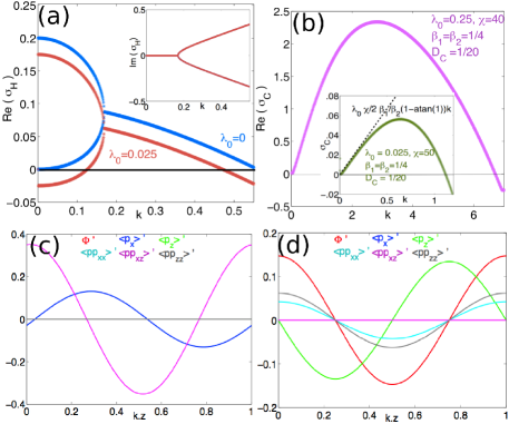
Figure 1: (color online) (a) The two branches of the growth rate obtained by the hydrodynamic relation. Inset shows the imaginary parts. (b) The growth rate obtained from the chemotaxis relation for $\lambda_{0}=0.25,\chi=40,\beta_{1}=\beta_{2}=1/4,D_{c}=1/20$. Inset shows the chemotaxis branch for parameters $\lambda_{0}=0.025,\chi=50,\beta_{1}=\beta_{2}=1/4,D_{c}=1/20$ used for simulations. The dashed line in the inset and its denoted slope are for a later comparison in Section IIID with the TP model. (c) Unstable eigenmodes or perturbations in the zeroeth, first and second moments of the distribution function w.r.t. the orientation vector $\mathbf{p}$ due to the hydrodynamics instability for wavenumber $\mathbf{k}=0.2\mathbf{\hat{k}}$ in a suspension of pushers with $\alpha=-1,\gamma=1$, and basal tumbling frequency $\lambda_{0}=0.025$. See Section IIIA-5 for an explanation. (d) Unstable eigenmodes or perturbations in the zeroth, first and second moments of the distribution function w.r.t. the orientation vector $\mathbf{p}$ due to the auto-chemotactic instability for wavenumber $\mathbf{k}=0.2\mathbf{\hat{k}}$ a suspension of swimmers with $\gamma=1$, $\lambda_{0}=0.025$, $\chi=50,\beta_{1}=\beta_{2}=1/4,D_{c}=1/20$.

For pushers ($\alpha<0$) there is a hydrodynamic instability for a finite band of wavenumbers $k\in[0,k_{c}\approx 0.55)$. Tumbling diminishes this range of unstable wave-numbers as the branch is brought down by $\lambda_{0}$ (again $Im(\sigma_{H})$ remains unaffected). From the numerical solution, we can estimate the critical wavenumber $k_{c}$ (and hence the critical system size $L_{c}=2\pi/k_{c}$) for which $Re(\sigma(k_{c}))=0$. Moreover, we can obtain a range of $\lambda_{0}$ for which a hydrodynamic instability is possible for pushers. We find that for $\lambda_{0}\geq 0.2$ there can be no hydrodynamic instability for any system size or swimmer shape (as represented by $\gamma$).

There are two positive $Re(\sigma_{H})$ branches which merge at $k\approx 0.19$, and at which the two conjugate branches of $Im(\sigma_{H})$ bifurcate from zero. This tells us that for $k<0.19$ we have two standing and growing modes, whereas beyond this the modes become complex.

For pullers, there is no hydrodynamic instability, as $Re(\sigma_{H}(k))<0$ even for $\lambda_{0}=0$ (see also SaintShelley08b ). The addition of basal tumbling $\lambda_{0}$ again shifts down the $Re(\sigma_{H})$ branches by $\lambda_{0}$ for all wavenumbers $k$ and further stabilizes the system. $Im(\sigma_{H})$ remains unchanged from the pusher case shown in Fig. 1a.

For the chemotactic dispersion relation, the long-wave asymptotics in Eq. (34) yields growth rate $\sigma_{C}\approx 1/(3\lambda_{0})[(\chi\beta_{2}/\beta_{1})\lambda_{0}-1]k^{2}+O(k^{4})$, which shows that for $(\chi\beta_{2}/\beta_{1})\lambda_{0}>1$ there are wavenumbers $k$ with $Re(\sigma_{C}(k))>0$, for pushers and pullers alike and for any swimmer shape parameter $\gamma$. Auto-chemotaxis thus introduces a new instability branch, which is solved numerically from Eq.(34) and plotted in Fig. 1b for two sets of $\lambda_{0},\chi,D_{c}$.

III.1.5 The Linear Perturbations

Using Eq. (37), and the numerical solution of the dispersion relations Eqs. (33, 34) for the parameters used in Fig. 1a & b, we have calculated the eigenmode using $\mathbf{\hat{k}}=\mathbf{\hat{z}}$ and $\mathbf{\hat{k}}_{\perp}=\mathbf{\hat{x}}$. We consider the hydrodynamic and auto-chemotactic contributions separately for $k=|\mathbf{k}|=0.2$. Fig. 1c & d illustrates the perturbations in the swimmer concentration $\Phi^{\prime}$ as well as the components of the first moment vector (also the un-normalized polarity vector) and second moment tensor (proportional to the active stress – neglecting the diagonal contribution) of the distribution function $\Psi$, namely $<\mathbf{p}>$ and $<\mathbf{pp}>$ for values of $kz=\mathbf{k}\cdot\mathbf{x}\in[0,1]$.

As seen in Fig. 1c, the hydrodynamic instability gives rise to perturbations in the director field $<\mathbf{p}>^{\prime}_{x}$ and the off-diagonal elements of the second moment of the distribution function w.r.t. the orientation vector, $<\mathbf{pp}>^{\prime}_{xz}$. The second moment is related to the active stress, as seen in Eq. (13), or linearized in Eq. (25), thus perturbations in the active stress do arise for non-zero $\alpha$. From Eq. (24) we expect nonzero perturbations in the fluid velocity to arise. (See also SaintShelley08b .) Perturbations due to the hydrodynamic instability are zero for the the other quantities, namely $\Phi^{\prime}$ $<\mathbf{p}>^{\prime}_{z}$, $<\mathbf{pp}>^{\prime}_{xx}$ and $<\mathbf{pp}>^{\prime}_{zz}$.

From Fig. 1d we see that the chemotactic instability gives rise to perturbations in the zeroeth moment of the distribution function (which is the swimmer concentration), the director field $<\mathbf{p}>^{\prime}_{z}$ and the diagonal elements of the second moment of the distribution function w.r.t. the orientation vector, $<\mathbf{pp}>^{\prime}_{xx}$ and $<\mathbf{pp}>^{\prime}_{zz}$, which are related to the normal stresses. Perturbations due to the chemotactic instability are zero for the other quantities, such as $<\mathbf{p}>^{\prime}_{x}$ and $<\mathbf{pp}>^{\prime}_{xz}$.

In the linearized system the hydrodynamic and chemotactic instabilities are uncoupled and operate independently in different directions. The hydrodynamic instability gives rise to shear stresses and a flux in the $\mathbf{\hat{k}}_{\perp}$ direction. Auto-chemotaxis gives rise to aggregation, a flux in the $\mathbf{\hat{k}}$ direction, and normal stresses. In the full non-linear system these perturbations and modes are of course coupled and interesting dynamics emerges from the interplay of these instabilities, as shown later with simulations.

III.2 A Phase Diagram of the Dynamics

Linear theory shows that there is a range of $\lambda_{0}$ for which there is a hydrodynamic instability in pusher suspensions. If $\lambda_{0}\geq 0.2$, there is no hydrodynamic instability for any system size and any swimmer shape $\gamma$, since, as seen in Fig. 1a, $Re(\sigma_{H}(k))\leq 0.2$. For an auto-chemotactic instability we need $(\chi\beta_{2}/\beta_{1})\lambda_{0}>1$. This connects the auto-chemotaxis parameters $\chi$, $\beta_{1}$, $\beta_{2}$ to the basal tumbling rate $\lambda_{0}$. This information about the parameters is assembled in a phase diagram in Fig. 2, which shows the parameters and various dynamical regimes we expect based on the linear theory and simulations.

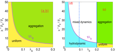
Figure 2: (Color online) Phase space of various regimes for auto-chemotactic and/or hydrodynamic instabilities in suspensions of pullers or neutral swimmers (left), and pushers (right) as a function of the basal tumbling frequency $\lambda_{0}$ and chemotactic parameters $\chi,\beta_{1},\beta_{2}$. Solid boundaries refer to the linear stability at long waves. Dashed lines show where we observe the boundaries to shift in simulations at finite box size. Red marks (a-d) indicate the parameters used for nonlinear simulations.

For pullers or neutral swimmer (right panel of Fig. 2) there are only two states: aggregation due to auto-chemotaxis and the uniform stable state. For pushers (right panel of Fig. 2), there are four dynamical regimes: aggregation (due to auto-chemotaxis), a regime where strong mixing fluid flows emerge (due to the hydrodynamic instability), a mixed state of both auto-chemotactic and hydrodynamic instabilities, and the uniform stable state where perturbations should decay to uniform isotropy. Other parameters, say the shape parameter $\gamma$, can alter this diagram.

III.3 Linear Stability of Turning-Particle Auto-Chemotaxis

The linear stability analysis of the Turning-Particle model of auto-chemotaxis is done in a similar manner, and the results obtained are remarkably similar to the Run-and-Tumble model with linearized tumbling rate, even though there is tumbling in this instance. For swimmers with no translational or rotational diffusion ($D=d_{r}=0$), the two dispersion relations are

$$1 =-\frac{3\alpha\gamma}{4ik}\left[2a_{H}^{3}-\frac{4}{3}a_{H}+(a_{H}^{4}-a_{H}^{2})\log\frac{a_{H}-1}{a_{H}+1}\right],$$ (40)

$$1 =\xi R\left[2+a_{C}\log\frac{a_{C}-1}{a_{C}+1}\right],$$ (41)

with $a=-i\sigma/k$. The long-wave (small $k$) asymptotics for the hydrodynamics relation yields $\sigma_{H1}=-\frac{\alpha\gamma}{5}+\frac{15}{7\alpha\gamma}k^{2}+...$ and $\sigma_{H2}=-\frac{1}{\alpha\gamma}k^{2}+...$ which is similar to the results found for the Run-and-Tumble model in Eqs. (III.1.3) without basal tumbling. The asymptotics of the auto-chemotactic relation gives $\sigma_{C}=\sigma_{1}k+\sigma_{3}k^{3}+...$ with $\sigma_{1}\approx\xi(1-\arctan(1))\beta_{2}/\beta_{1}$ and $\sigma_{3}\approx D_{c}/\beta_{1}$. While this does not look similar to the Run-and-Tumble result in Eq. (III.1.3), the numerical solution in Fig. 3 shows similarities in the overall curve shape, maxima and critical $k_{c}$ where $\sigma(k_{c})=0$.

Moreover, a finite band of wavenumbers with $Re(\sigma_{C})>0$ can be found for $k\in[0,k_{c}=\sqrt{(2\xi\beta_{2}-\beta_{1})/D_{c})}]$. For this model we can as well express the eigenmodes for the distribution function as linear combinations of the form in Eq. (35) with the eigenvector arising from chemotaxis in the $\mathbf{\hat{k}}$ direction and the eigenvector arising from the hydrodynamics perpendicular to $\mathbf{\hat{k}}$. It can also be shown that the hydrodynamic instability increases growth of the shear stresses whereas the auto-chemotactic instability increases fluctuations in the swimmer concentration and normal stresses.

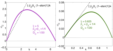
Figure 3: (color online) The growth rate for the Turning-Particle auto-chemotaxis relation: $\xi=5$ (left) and $\xi=0.625$ (right) with $\beta_{1}=\beta_{2}=1/4,D_{c}=1/20$. Dashed lines show the long-wave asymptotics. Parameters $\xi$ are chosen so that $\xi=\lambda_{0}\chi/2$ with $\lambda_{0},\chi$ corresponding to those shown in Fig.1b. The comparison is discussed in Section IIID.

Although not shown here, including translational diffusion with constant $D$ merely shifts down the $Re(\sigma_{H})$ and $Re(\sigma_{C})$ by $-Dk^{2}$ (see SaintShelley08b for non-tumbling non-chemotactic swimmers). As found by HohenShelley10 , when rotational diffusion with constant $d_{r}$ is included in the stability analysis of non-chemotactic swimmers, the hydrodynamic instability branch $Re(\sigma_{H})$ shifts down by approximately $6d_{r}$ for small $k$. We do not discuss here how non-zero rotational diffusion $d_{r}$ affects the chemotactic instability.

III.4 Relating the Two Chemotaxis Models

In the Run-and-Tumble chemotaxis model, tumbling helps stabilize the the system; the hydrodynamic instability branches are shifted downwards by the basal tumbling frequency $\lambda_{0}$, as seen in Fig. 1. And, as just mentioned above, rotational diffusion shifts down the hydrodynamic instability branches in non-chemotactic suspensions by approximately $6d_{r}$ HohenShelley10 ; LushiDissert for $k\ll 1$. In this respect, at large system sizes tumbling with basal frequency $\lambda_{0}$ acts like rotational diffusion with coefficient $6d_{r}$.

Comparing the first terms of the two chemotactic dispersion relations, Eqs. (34) & (41), suggests that $\xi\approx\lambda_{0}\chi/2$ relates the behavior of the RT model with basal tumbling $\lambda_{0}$ and chemotactic strength $\xi$ to the behavior of the TP chemotaxis model with strength $\xi$. Since in the $k\ll 1$ regime the chemotactic growth rate of the TP model is $\sigma_{C}\approx\xi(1-\arctan(1))\beta_{2}/\beta_{1}k$, we plot the line with slope $\lambda_{0}\chi/2(1-\arctan(1))\beta_{2}/\beta_{1}$ in Fig. 1b and see that it gives a good approximation to the growth rate from the RT model in the $k\ll 1$ limit. Comparison of the curves in Fig. 1b for the RT model and Fig. 3 for the TP model, when the chemotactic parameters are matched as such, shows also their similarity in overall curve shape, maxima and critical wave-numbers $k_{c}$ where $\sigma(k_{c})=0$. The eigenmodes of the two models also have a very similar structure.

Thus, for $k\ll 1$, the linearized TP model with chemotactic parameter $\xi$ and rotational diffusion $d_{r}$ behaves similarly to the linearized RT model with basal tumbling $\lambda_{0}$ and chemotactic sensitivity $\chi$, when the parameters are related as $\xi\approx\lambda_{0}\chi/2$ and $\lambda_{0}=6d_{r}$. Full nonlinear simulations for box sizes corresponding to $k\ll 1$ and with parameters chosen as above support this matching, as is shown in the next section.

IV Nonlinear Simulations

In full simulations we focus primarily on the Run-and-Tumble model, leaving the Turning-Particle model for comparison at the end, but noting we expect similar dynamics when the parameters are properly matched as explained in Section IIID. Using simulation we investigate the system dynamics in the various regimes suggested by phase diagram in Fig. 2. Of particular interest is the aggregation regime for different types of swimmers, and the mixed dynamics regime of pusher suspensions.

IV.1 Numerical Method

For relative ease of simulation we consider 2D doubly periodic systems in which the particles are constrained to the $(x,y)$-plane with orientation parametrized by an angle $\theta\in[0,2\pi)$ so $\mathbf{p}=(\cos\theta,\sin\theta,0)$. Since all the dependent variables are periodic in $x$, $y$ and $\theta$ we use discrete Fourier transforms (via the FFT algorithm) to approximate spatial and angular derivatives and to solve the flow equations Eq. (II.1). Integrations in $\theta$ to obtain the swimmer density $\Phi$ (15) and active particle stresses $\Sigma^{a}$ [Eq. (13)] use the trapezoidal rule, which is spectrally accurate in this instance. Usually $128-256$ points are used in the $x$ and $y$ directions and $32-64$ in the $\theta$ direction. We integrate the distribution equation Eq. (1) and the chemo-attractant advection-diffusion equation Eq. (16) using a second-order time-stepping scheme (Adams-Bashforth/Crank-Nicholson). Particle translational and rotational diffusion and chemo-attractant diffusion are included in all simulations for numerical stability (values of $D=d_{r}=0.025$ and $D_{c}=0.05$ were used in most simulations). All results presented are for slender micro-organisms with $\gamma=1$ and the spatial square box side is $L=50$. The initial swimmer distribution is taken to be a uniform and isotropic suspension perturbed as

$$\Psi(\mathbf{x},\theta,0)=\frac{1}{2\pi}\left[1+\sum_{i}\epsilon_{i}\cos(\mathbf{k}_{i}\cdot\mathbf{x}+\xi_{i})P_{i}(\theta)\right],$$ (42)

where $\epsilon_{i}$ is a small random coefficient ($\epsilon_{i}\in[-0.01,0.01]$), $\xi_{i}$ is a random phase and $P_{i}(\theta)$ is a third-order polynomial of $\sin\theta$ and $\cos\theta$ with random $O(1)$ coefficients. The initial chemo-attractant concentration is taken to be uniform and $C(\mathbf{x},0)=\beta_{2}/\beta_{1}$ with $\beta_{1}=\beta_{2}$ used for most simulations.

IV.2 Chemotaxis-Driven Dynamics

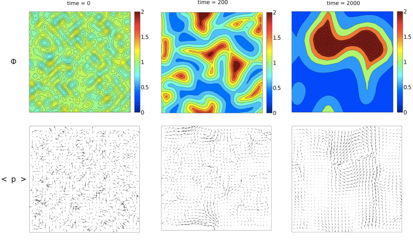
Figure 4: (Color online) Auto-chemotaxis in a neutral swimmer suspension at times $t=$0, 200, and 2000. The first row shows concentration of swimmers $\Phi$, the second row shows the swimmer mean direction $<\mathbf{p}>$. At $t=$200, $max|<\mathbf{p}>|=0.091$ and at $t=$2000, $max|<\mathbf{p}>|=0.086$.

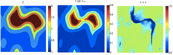
Figure 5: (Color online) Auto-chemotaxis in a neutral swimmer suspension at time $t=2000$. Shown are the chemoattractant concentration $C$, the diagonal entry $<\mathbf{pp}>_{xx}$ of the second moment tensor of the distribution function, and the mean tumbling frequency $<\lambda(\mathcal{D}_{t}C)>$.

To illustrate the effect of pure auto-chemotaxis in the absence of hydrodynamics, we first simulate a suspension of theoretical neutral swimmers by setting $\alpha=0$. The other parameters used are $\lambda_{0}=0.25$, $\chi=40$, $\beta_{1}=\beta_{2}=1/4$ for which the linear stability analysis suggests an aggregation instability – see the red mark (a) in the phase diagram of Fig. 2. Fig. 4 shows plots of the swimmer concentration $\Phi$ and mean direction $<\mathbf{p}>=\int d\mathbf{p^{\prime}}\Psi(\mathbf{p^{\prime}})\mathbf{p^{\prime}}/\Phi$ at times $t=$0, 200, and 2000. The chemo-attractant concentration field $C$, the diagonal entry $<\mathbf{pp}>_{xx}$ of the second moment tensor (related to the active stress, were it present in this case), and the mean tumbling rate $<\lambda(\mathcal{D}_{t}C)>$, are shown at $t=2000$ in Fig. 5.

The swimmer concentration field in Fig. 4 shows continual aggregation and coarsening. At late times ($t=2000$) the swimmers have aggregated into a single still-evolving doubly-peaked irregular mass. The chemo-attractant field closely follows the swimmer concentration as seen in Fig. 5, with the two plots being nearly identical to the eye. Indeed, this observation supports the validity of the approximation of a quasi-static chemo-attractant field in the linear stability analysis. Note that $<\mathbf{pp}>_{xx}$ is also similar to the swimmer concentration field, being significant only in the aggregation regions, suggesting a link between hydrodynamic interactions (were they present) and chemotactic aggregation. Within the aggregation region the chemo-attractant gradient is steep and the mean tumbling frequency $<\lambda(\mathcal{D}_{t}C)>$ is less than the basal frequency $\lambda_{0}$, suggesting further swimmer aggregation and coarsening.

While continual aggregation is observed, there is little sign of the rapid self-focussing associated with the finite-time chemotactic collapse Childress84 ; JagerLuck92 ; DolPert04 seen in the KS model. Here that may in part be due to the constant swimming speed of individual particles SchnitzerEtAl90 .

IV.3 Auto-chemotaxis of Puller Suspensions

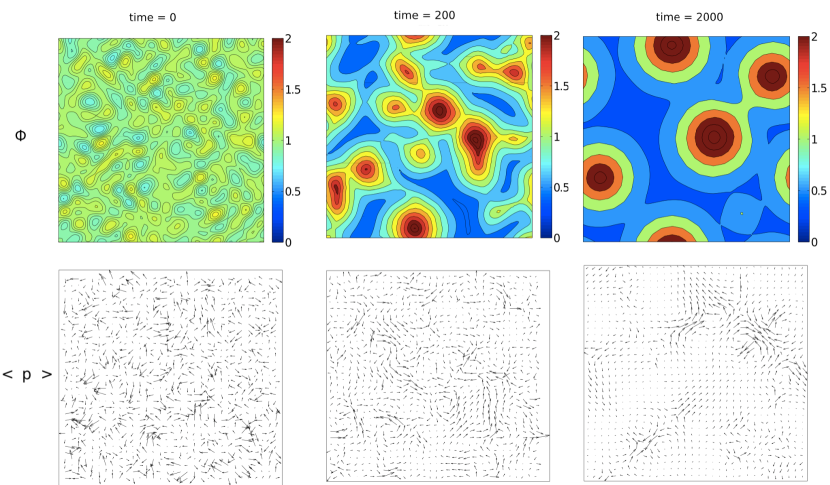
Figure 6: (Color online) Auto-chemotaxis in a puller swimmer suspension at times $t=0,200,2000$. The first row shows concentration of swimmers $\Phi$, the second row shows the swimmer mean direction $<\mathbf{p}>$. At $t=$200, $max|<\mathbf{p}>|=0.085$ and at $t=$2000, $max|<\mathbf{p}>|=0.067$.

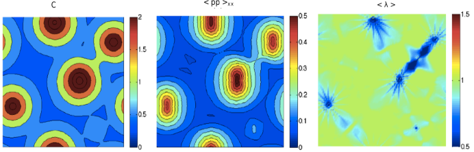
Figure 7: (Color online) Auto-chemotaxis in a puller swimmer suspension at time $t=2000$. Shown are the chemoattractant concentration $C$, the diagonal entry $<\mathbf{pp}>_{xx}$ of the second moment tensor of the distribution function, and the mean tumbling frequency $<\lambda(\mathcal{D}_{t}C)>$.

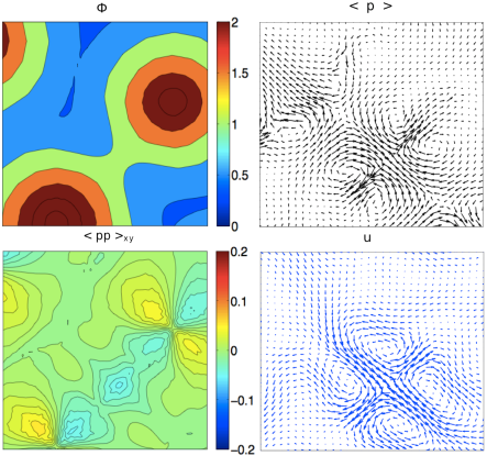
Figure 8: (Color online) Closeup of the top-right quarter of the domain of the auto-chemotactic puller suspension dynamics at time $t=2000$ as shown in Fig. 6. Top: the swimmer concentration $\Phi$ and mean direction $<\mathbf{p}>$ with $max|<\mathbf{p}>|=0.067$. Bottom: the off-diagonal entry of the second moment tensor $<\mathbf{pp}>_{xy}$ (related to the active stress) and the generated fluid velocity $\mathbf{u}$ with $max|\mathbf{u}|=0.03$.

We next perform the same numerical experiment but with a suspension of pullers (setting $\alpha=1$). The other system parameters remain unchanged – see the red mark (b) in the phase diagram of Fig. 2. Linear stability analysis suggests an aggregation instability due to auto-chemotaxis, but with hydrodynamical interactions suppressed since the growth rates in the hydrodynamic instability have negative real part. The results are illustrated in Figs. 6 and 7.

Fig. 6 for time $t=200$ shows that initial aggregation and coarsening occurs in this suspension of pullers in a way very similar to that of neutral swimmers. The swimmers aggregate into a few regions that merge and grow. As before, the chemo-attractant concentration field closely follows swimmer concentration, and $<\mathbf{pp}>_{xx}$ (related to the active first normal stress) is significant in the aggregation regions. There is a chemo-attractant spatial gradient in the aggregation regions at early times and the swimmer mean tumbling frequency there is less than the basal frequency $\lambda_{0}$, suggesting the swimmers are on average moving toward higher values of chemoattractant concentration.

However major differences from the neutral swimmer case eventually emerge in the pattern morphology. At late times ($t=2000$) the aggregation regions have become circular and there is no indication of further coarsening. Indeed, these circular regions are all of a similar size and appear to be mutually repelling, suggesting that this is the terminal state of the system. Obviously the hydrodynamic interactions have made a large difference. What is happening can be partially explained by examining the fluid velocity field $\mathbf{u}$ and the off-diagonal element of the second moment tensor $<\mathbf{pp}>_{xy}$ (related to the the shear active stresses) in the region between two circular aggregates (see Fig. 8). Though small in magnitude, the fluid flow is non-trivial and persistent, and $<\mathbf{pp}>_{xy}$ is close in magnitude to $<\mathbf{pp}>_{xx}$. Most importantly, observe that in the saddle point regions between the circular aggregates the fluid flows are such that they keep the aggregates apart. By this mechanism, the hydrodynamic interactions between the aggregates seem to have slowed down, if not stopped altogether, further aggregation and coarsening.

IV.4 Auto-chemotaxis of Pusher Suspensions

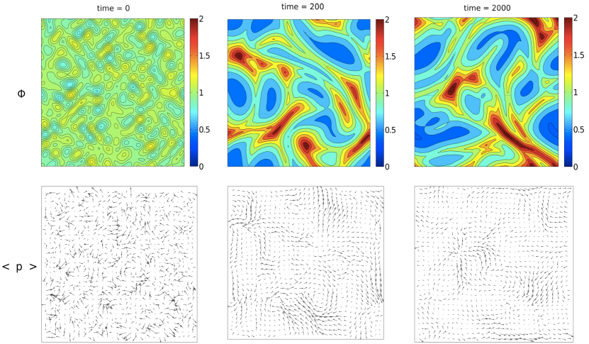
Figure 9: (Color online) Auto-chemotaxis in a pusher swimmer suspension at times $t=0,200,2000$. The first row shows concentration of swimmers $\Phi$, the second row shows the swimmer mean direction $<\mathbf{p}>$.At $t=$200, $max|<\mathbf{p}>|=0.111$ and at $t=$2000, $max|<\mathbf{p}>|=0.118$

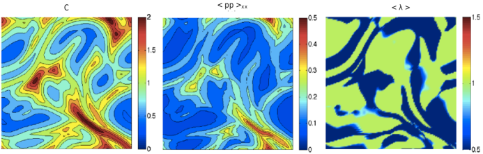
Figure 10: (Color online) Auto-chemotaxis in a pusher swimmer suspension at time $t=2000$. Shown are the chemoattractant concentration $C$, the diagonal entry $<\mathbf{pp}>_{xx}$ of the second moment tensor of the distribution function, and the mean tumbling frequency $<\lambda(\mathcal{D}_{t}C)>$.

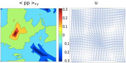
Figure 11: (Color online) Auto-chemotactic pusher suspension dynamics at time $t=2000$ as shown in Fig. 9. Left: the off-diagonal entry of the second moment tensor $<\mathbf{pp}>_{xy}$ (related to the active stress). Right: the generated fluid velocity $\mathbf{u}$ with $max|\mathbf{u}|=0.87$.

We now consider the same numerical experiment for a suspension of pushers (setting $\alpha=-1$), again keeping all the other parameters the same – see the red mark (c) in the phase diagram of Fig. 2. Linear stability analysis suggests an aggregation instability due to auto-chemotaxis, and the value of $\lambda_{0}$ is large enough to suppress the hydrodynamic linear instability (refer to Fig. 1a and shift down the hydrodynamic instability branches by $\lambda_{0}=0.25$, making all eigenvalues negative).

In Figs. 9 and 10 we see that at earlier times the dynamics is dominated by aggregation into regions of high swimmer concentration, as in the neutral swimmer and puller cases. However, swimmer concentration also leads to locally increased active stresses which create strong destabilizing fluid flows. These unsteady fluid flows are significant in magnitude and macroscopic in scale, and push around the regions of concentrated swimmers and the chemo-attractant. The resulting dynamics is one of fragmented regions of aggregation and constant flow instability, seemingly chaotic in nature. The flows have apparently suppressed further growth in the swimmer concentration.

To reinforce this point, we plot in Fig. 12a the maximum of the fluid velocity. This shows that the fluid flow is of significant magnitude, especially considering that this is for parameters for which linear stability analysis predicted no fluid flows at all. The viscous dissipation $\mathbf{S}=\int d\mathbf{x}\mathbf{E}:\mathbf{E}$, which contributes positively to the system configurational entropy in pusher suspensions (see its significance explained in SaintShelley08b ), is shown in Fig. 12b.

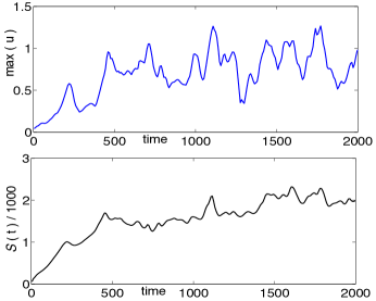
Figure 12: (Color online) The maximum fluid speed $max(|\mathbf{u}|)$ (top) and the configurational entropy $\mathit{S}$ (bottom) vs. time for the auto-chemotactic pusher suspension shown in Fig. 9.

IV.5 Interactions Limit Chemotactic Growth

As noted above, hydrodynamic interactions can alter auto-chemotactic growth significantly. To quantify this we track the maximum of the swimmer concentration $\Phi$ and the the configurational entropy $\mathit{S}=\int d\mathbf{x}\int d\mathbf{p}(\Psi/\Psi_{0})\log(\Psi/\Psi_{0})$ in Fig. 13. We observe that these two quantities continually increase for suspensions of neutral swimmers, but seem to be capped for the suspensions of pullers or pushers. The chemotactic growth here is bounded by the hydrodynamical interactions and the fluid flows the swimmers generate.

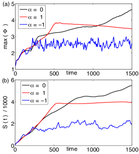
Figure 13: (Color online) (a) Comparisons in the maximum swimmer concentration $\Phi$, and (b) configurational entropy $\mathit{S}$ in the neutral swimmer ($\alpha=0$, Fig. 4), puller ($\alpha=1$, Fig. 6) and pusher ($\alpha=-1$, Fig. 9) suspensions with otherwise the same chemotactic parameters.

IV.6 Mixed Dynamics in Pusher Suspensions

It is well-known that pusher suspensions ($\alpha<0$) develop a hydrodynamic instability SaintShelley08 ; SaintShelley08b ; SubKoch09 . In that case without chemotaxis, the nonlinear dynamics produces concentration bands that stretch and fold in a quasi-periodic manner, giving rise to strongly mixing fluid flows. We now investigate what happens to the suspension dynamics when auto-chemotaxis is included. This corresponds to the “mixed dynamics” area in the phase diagram for pushers in Fig. 2a.

For this purpose, we perform nonlinear simulations with $\lambda_{0}=0.025$, $\chi=50$, $\beta_{1}=\beta_{2}=1/4$, $D_{c}=0.05$, for which linear theory predicts dynamics with both strong auto-chemotactic and hydrodynamic instabilities (see red marker (d) in the phase diagram of Fig. 2). For comparison we include the cases of purely-tumbling suspensions ($\lambda_{0}=0.025,\chi=0$), non-chemotactic suspension ($\lambda_{0}=0$), and another case for which linear analysis predicts just hydrodynamic, but no auto-chemotactic instability (with $\lambda_{0}\chi\beta_{2}/\beta_{1}<1$).

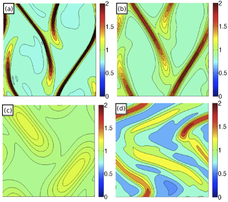
Figure 14: (color online) Swimmer concentration $\Phi$ in pusher suspensions that are: (a) strongly auto-chemotactic $\lambda_{0}=0.025$, $\chi=50$, (b) weakly auto-chemotactic $\lambda_{0}=0.025$, $\chi=35$ ($\lambda_{0}\chi\beta_{2}/\beta_{1}<1$), (c) purely tumbling but non-chemotactic $\lambda_{0}=0.025$, $\chi=0$, and (d) non-tumbling and non-chemotactic $\lambda_{0}=0$.

Fig. 14 shows plots of the swimmers concentration at the onset of the mixing regime. Auto-chemotactic swimmers produce chemo-attractant as well as aggregate towards it. A strongly mixing flow emerges and advects both swimmers and chemo-attractant. The chemo-attractant dynamics closely follows those of the swimmer concentration, resulting in dynamic aggregation of swimmers occurring due to the local auto-chemotactic tendency. This effect is seen from the sharper and narrower concentration bands in the auto-chemotactic suspension in Fig. 14a compared to non-chemotactic tumblers in Fig. 14c. Hence auto-chemotaxis stabilizes the formation of concentration bands that pure tumbling had diminished through its diffusion-like effect. The effect is apparent even for the case where no auto-chemotactic instability is predicted by linear theory ($\lambda_{0}\chi\beta_{2}/\beta_{1}<1$), as shown in Fig. 14b. In Fig. 14a-d we see that auto-chemotaxis has also hastened the onset of the mixing regime when compared to the purely-tumbling pusher suspension. Linear stability predicts that pure tumbling has a stabilizing effect on the suspension. This is confirmed in simulations when comparing the weak concentration bands for pure-tumbler compared to the non-tumbling suspension of non-chemotactic pushers in Fig. 14cd. These effects are also illustrated in plots of the swimmer concentration and generated fluid flow in Fig. 15.

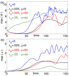
Figure 15: (color online) Dynamics in pusher suspensions of Figs.  14a-c: (a) maximum of the swimmer concentration $\Phi$, (b) maximum of the fluid speed $\mathbf{u}$.

IV.7 Similarities between the Chemotaxis Models

We illustrate the qualitative similarities in the dynamics of the two chemotaxis models when the parameters are matched as suggested by the linear theory: $\lambda_{0}\approx 6d_{r}$ and $\xi\approx\lambda_{0}\chi/2$. Fig. 16 shows pusher swimmer concentration for the two models at the onset of mixing. The profiles and dynamics are remarkably similar, and such similarity is also observed in plots of chemo-attractant, the generated fluid flows, and the normal and shear stresses (not shown).

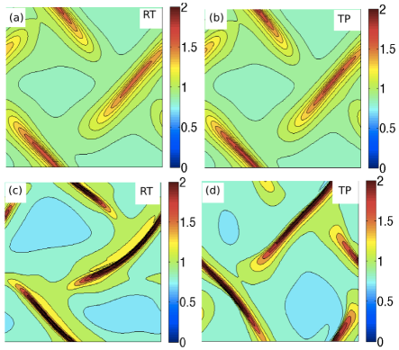
Figure 16: (color online) Swimmer concentration $\Phi$ in pusher suspensions for the RT chemotaxis model with $\lambda_{0}=0.025,\chi=60,d_{r}=0.025$ (left) and TP chemotaxis model with $\xi=0.75,d_{r}=0.175$ (right) at times $t=100$ (top) and $t=150$ (bottom).

The Turning-Particle model assumes that a swimmer is able to detect the local chemo-attractant gradient and adjust its orientation to swim towards the regions of high chemo-attractant concentration. This chemotactic response is induced through a torque that aligns the swimmers with the chemo-attractant gradient. While the model is not applicable to bacteria, it is interesting that there are connections to the Run-and-Tumble chemotaxis model in the linear analysis and the also the nonlinear dynamics in the long wave regimes. This connection might be helpful in designing models for direct swimmer simulations of chemotactic response. On that note, approaches that model chemotaxis as a bias in the swimmer direction have been applied in other studies of individual swimmer models DillonEtAl95 ; HopkinsFauci02 ; TaktikosEtAl12 .

V Discussion and Conclusion

We have presented and elaborated upon two kinetic models that couple chemo-attractant production and response in colonies of micro-swimmers with the fluid flows that the swimmers collectively generate by their motion. These models, and our study of them, merge together two separate areas of investigation: chemotactic aggregation due to population-produced chemo-attractants, and the hydrodynamics of active motile suspensions. In classical models of attractive chemotaxis, concentration through aggregation is often unbounded and can blow up in finite time, and such behaviors are sometimes avoided in extended models through the inclusion of ad hoc saturation terms. We show here that the flows generated by motile suspensions can also limit aggregation growth, though for very different reasons depending upon the swimmer type. That the collective flows associated with motility can achieve this has not been previously demonstrated.

Still, the application of our modeling may be limited. Our active suspension model is a dilute to semi-dilute theory that does not include local interactions between swimmers, either hydrodynamic or steric; see CisnEtAl11 ; DrescherEtAl11 ; Dunkel13 ; Hensink12 ; SokolovAranson12 for relevant experiments using bacteria. In denser suspensions the swimmer size limits local swimmer density through steric interactions, and well-founded models that combine these with hydrodynamic interactions are in development (for one recent attempt, see Ezhilan13 ). We do note a recent study by Taktikos et. al. TaktikosEtAl12 for discrete disk-shaped chemotactic random walkers in 2D with steric but no hydrodynamic effects showing that steric interactions can limit aggregation, as indeed they must. Further, in dense suspensions it is not clear how run-and-tumble dynamics, as has been observed and modeled, is affected by crowding and steric interactions. Intuitively, one expects the swimmer tumbling frequency to decrease in denser suspensions where mobility is limited due to crowding.

While these theoretical results on the coupling of auto-chemotaxis with collectively-generated flows have not yet been systematically studied in an experimental setting, this might be possible with the specific engineering of the dynamics of locomotion and chemosensing ParkEtAl03 . Moreover, the interplay between locomotion, fluid flows, chemotaxis and quorum sensing can be further illuminated through the controlled introduction of exogenous chemo-attractants LiuEtAl11 . As a relevant example, a recent experiment by Saragosti et. al. SaragostiEtAl11 used exogenous chemo-attractants in conjunction with those produced by swimming E. coli to induce aggregation and traveling waves of bacteria in a channel. As side-note on this, in our first study (Lushi et. al. LGS12 ) we investigated the RT model using parameters close to those of the Saragosti et al SaragostiEtAl11 experiment and found the production of filamentary aggregates (see Fig. 1(iv) and Supplementary Material of LGS12 ). Despite this system being well outside of the regime of hydrodynamic instability (as predicted by our linear analysis), hydrodynamics was plainly important in their local dynamics. Perhaps in a setting that also included the effects of confinement and steric ordering, these aggregates would transition to traveling waves. Obviously this model is easily modified to study the effects of external chemo-attractants (see, for example, Ezhilan12 ; LushiDissert ). Chemotaxis in bacterial colonies has been previously exploited for enhancing mixing in microfluidic devices KimBreuer07 , but it has not yet been studied experimentally how the mixing process might be affected by auto-chemotaxis. Lastly, chemotactic-like behavior is also observed in suspensions of synthetic micro-swimmers that exist in micro-fluidic environments (see HongEtAl07 for experiments, and TBZS2013 ; MWAP2013 for recent theory). Such chemotactic responses might be exploited in the future in technological applications HongEtAl07 ; Kagan10 ; SenVel09 .

- (1) W. Alt. “Biased random walk models for chemotaxis and related diffusion approximations.”, J. Math. Bio. 9, 147, (1980).
- (2) B.L. Bassler. “Small talk. Cell-to-cell communication in bacteria.” Cell 109, 421 (2002).
- (3) R.N. Bearon and T.J. Pedley. “Modeling run-and-tumble chemotaxis in a shear flow.” Bull. Math. Bio. 62, 775 (2000).
- (4) H.C. Berg. Random Walks in Biology. Expanded Ed., Princeton University Press (1993).
- (5) H.C. Berg and D.A. Brown. “Chemotaxis in Escherichia Coli analyzed by three-dimensional tracking.” Nature, 239, 500 (1972).
- (6) E.O. Budrene and H.C. Berg. “Complex patterns formed by motile cells of Escherichia Coli.” Nature 349, 630 (1991).
- (7) E.O. Budrene and H.C. Berg. “Dynamics of formation of symmetrical patterns by chemotactic bacteria” Nature 376, 49 (2002).
- (8) K.C. Chen, R.M. Ford, and P.T. Cummings. “Cell balance equation for chemotactic bacteria with a biphasic tumbling frequency.” J. Math. Bio. 47, 518 (2003).
- (9) S. Childress. “Chemotactic collapse in two dimensions.” Lecture Notes in Biomath. Springer, Berlin. 55, 61 (1984).
- (10) L. Cisneros, R. Cortez, C. Dombrowski, R.E. Goldstein, and J.O. Kessler. “Fluid dynamics of self-propelled microorganisms, from individuals to concentrated populations.” Exp. Fluids 43, 737 (2007).
- (11) L.H. Cisneros, J.O. Kessler, S. Ganguly, and R.E. Goldstein. “Dynamics of swimming bacteria: Transition to directional order at high concentration.” Phys. Rev. E 83, 061907 (2011).
- (12) R. Dillon, L. Fauci, and D. Gaver. “A micro-scale model of bacterial swimming, chemotaxis and substrate transport.” J. Theor. Biol. 177, 325 (1995).
- (13) M. Doi and S.F. Edwards. The Theory of Polymer Dynamics, Oxford University Press, Oxford (1986).
- (14) J. Dolbeault and B. Perthame. “Optimal critical mass in the two-dimensional Keller-Segel model in .” C.R. Math. Acad. Sci. Paris 339, 611 (2004).
- (15) C. Dombrowski, L. Cisneros, S. Chatkaew, R. E. Goldstein, and J. O. Kessler. “Self-concentration and large-scale coherence in bacterial dynamics.” Phys. Rev. Lett. 93, 098103 (2004).
- (16) K. Drescher, J. Dunkel, L.H. Cisneros, S. Ganguly, and R.E. Goldstein, “Fluid dynamics and noise in bacterial cell-cell and cell-surface scattering.” Proc. Natl. Acad. Sci. USA 108, 10940 (2011).
- (17) J. Dunkel, S. Heidenreich, K. Drescher, H.H. Wensink, M. Bar, and R.E. Goldstein “Fluid dynamics of bacterial turbulence.” Phys. Rev. Lett. 110, 228102 (2013)
- (18) B. Ezhilan, A. Pahlavan, D. Saintillan. “Chaotic dynamics and oxygen transport in thin films of aerotactic bacteria” Phys. Fluids 24, 091701 (2012) (2012).
- (19) B. Ezhilan, M. J. Shelley, D. Saintillan. “Instabilities and nonlinear dynamics of concentrated active suspensions.” submitted. (2013).
- (20) H. H. Wensink, J. Dunkel, S. Heidenreich, K. Drescher, R.E. Goldstein, H. Lowen, and J.M. Yeomans, Meso-scale Turbulence in Living Fluids. Proc. Natl. Acad. Sci. U.S.A. 109, 14308 (2012).
- (21) N.A. Hill and T.J. Pedley. “Bioconvection.” Fluid Dyn. Res. 37, 1 (2005).
- (22) C. Hohenegger and M.J. Shelley. “On the stability of active suspensions.” Phys. Rev. E 81, 046311 (2010).
- (23) Y. Hong, N.M.K. Blackman, N.D. Kopp, A. Sen and D. Velegol “Chemotaxis of non-biological nanorods.” Phys. Rev. Lett. 99, 178103 (2007).
- (24) M.M. Hopkins and L.J. Fauci. “A computational model of the collective fluid dynamics of motile micro-organisms.” J. Fluid Mech. 455, 149 (2002).
- (25) W. Jager and S. Luckhaus. “On explosions of solutions to a system of partial differential equations modelling chemotaxis.” Trans. Amer. Math. Soc. 329 819 (1992).
- (26) G. B. Jeffrey. “The motion of ellipsoidal particles immersed in a viscous fluid.” Proc. R. Soc. London, Ser. A 102, 161 (1922).
- (27) D. Kagan, R. Laocharoensuk, M. Zimmerman, C. Clawson, S. Balasubramanian, D. Bishop, S. Sattayasamitsathit, L. Zhang and J. Wang. “Rapid Delivery of Drug Carriers Propelled and Navigated by Catalytic Nanoshuttles.” Small 6, 2741 (2010).
- (28) E.F. Keller and L.A. Segel. “Initiation of slime mold aggregation viewed as an instability.” J. Theor. Biol. 26, 399 (1970).
- (29) E.F. Keller and L.A. Segel. “Model for chemotaxis.” J. Theor. Biol. 30, 225 (1971).
- (30) M.J. Kim and K.S. Breuer “Controlled mixing in microfluidic systems using bacterial chemotaxis” Anal. Chem. 79, 955 (2007).
- (31) K.C. Leptos, J.S. Guasto, J.P. Gollub, A.I. Pesci, and R.E. Goldstein “Dynamics of enhanced tracer diffusion in suspensions of swimming eukaryotic microorganisms” Phys. Rev. Lett. 103, 198103 (2009).
- (32) C. Liu, X. Fu, L. Liu, X. Ren, C.K.L. Chau, S. Li, L. Xiang, H. Zeng, G. Chen, L.-H. Tang, P. Lenz, X. Cui, W. Huang, T. Hwa, and J.-D. Huang. “Sequential establishment of stripe patterns in an expanding cell population.” Science 334, 238 (2011).
- (33) E. Lushi. “Chemotaxis and other effects in active particle suspensions.” Ph.D. dissertation, New York University, (2011).
- (34) E. Lushi, R.E. Goldstein and M.J. Shelley. “Collective chemotactic dynamics in the presence of self-generated fluid flows.” Phys. Rev. E 86, 040902(R), (2012).
- (35) R.M. Macnab and D.E. Koshland. “The gradient-sensing mechanism in bacterial chemotaxis.” Proc. Natl. Acad. Sci. USA 69, 2509 (1972).
- (36) N. Marine, P. Wheat, J. Ault, and J. Posner “Diffusive behaviors of circle-swimming motors” Phys. Rev. E 87, 052305 (2013).
- (37) N. Mittal, E.O. Budrene, M.P. Brenner and A. van Oudenaarden, “Motility of Escherichia Coli cells in clusters formed by chemotaxis.” Proc. Natl. Acad. Sci. USA 100, 13259 (2003).
- (38) S. Park, P.M. Wolanin, E.A. Yuzbashyan, P. Silberzan, J.B. Stock, and R.H. Austin, “Motion to form a quorum.” Science 301, 188 (2003).
- (39) T.J. Pedley and J.O. Kessler. “Hydrodynamic phenomena in suspensions of swimming microorganisms.” Annu. Rev. Fluid Mech. 24, 313 (1992).
- (40) I. Rushkin, V. Kantsler, and R.E. Goldstein “Fluid velocity fluctuations in a suspension of swimming protists” Phys. Rev. Lett. 105, 188101 (2010).
- (41) D. Saintillan and M.J. Shelley. “Instabilities and pattern formation in active particle suspensions: Kinetic theory and continuum simulations.” Phys. Rev. Lett 100, 178103 (2008).
- (42) D. Saintillan and M.J. Shelley. “Instabilities, pattern formation, and mixing in active suspensions.” Phys. Fluids 20, 123304 (2008).
- (43) J. Saragosti, V. Calvez, N. Bournaveas, B. Perthame, A. Buguin and P. Silberzan, “Directional persistence of chemotactic bacteria in a traveling concentration wave.” Proc. Natl. Acad. Sci. USA 108, 16235 (2011).
- (44) M.J. Schnitzer. “Theory of continuum random walks and application to chemotaxis.” Phys. Rev. E 48, 2553 (1993).
- (45) M.J . Schnitzer, S.M. Block, H.C. Berg, and E.M. Purcell. “Strategies for chemotaxis.” Symp. Soc. Gen. Microbiol. 46, 15 (1990).
- (46) A. Sen, M. Ibele, Y. Hong, and D. Velegol. “Chemo and phototactic nano/microbots.” Faraday Discuss. 143, 15-27 (2009).
- (47) A. Sokolov and I.S. Aranson. “Physical properties of collective motion in suspensions of bacteria.” Phys. Rev. Lett. 109, 248109 (2012)
- (48) A. Sokolov, R.E. Goldstein, F.I. Feldstein and I.S. Aranson. “Enhanced mixing and spatial instability in concentrated bacteria suspensions.” Phys. Rev. E 80, 031903 (2009).
- (49) G. Subramanian and D.L. Koch. “Critical bacterial concentration for the onset of collective swimming.” J. Fluid Mech. 632, 359 (2009).
- (50) S. Sundararajan, S. Sengupta, M. Ibele, and A. Sen “Drop-off of colloidal cargo transported by catalytic Pt-Au nanomotors via photochemical stimuli” Small 6, 1479 (2010).
- (51) D. Takagi, A. Braunschweig, J. Zhang, and M. Shelley. “Dispersion of Self-Propelled Rods Undergoing Fluctuation-Driven Flips” Phys. Rev. Lett. 110, 038301 (2013).
- (52) J. Taktikos, V. Zaburdaev, and H. Stark. “Collective dynamics of model microorganisms with chemotactic signaling.” Phys. Rev. E 85, 051901 (2012).
- (53) M.J. Tindall, P.K. Maini, S.L. Porter, and J.P. Armitage. “Overview of mathematical approaches used to model bacterial chemotaxis ii: bacterial populations.” Bull. Math. Bio. 70, 1570 (2008).