Higgs Boson Cross Section from CTEQ-TEA Global Analysis

Abstract

We study the uncertainties of the Higgs boson production cross section through the gluon fusion subprocess at the LHC (with $\sqrt{s}=7,8$ and $14$ TeV) arising from the uncertainties of the parton distribution functions (PDFs) and of the value of the strong coupling constant $\alpha_{s}(M_{Z})$. These uncertainties are computed by two complementary approaches, based on the Hessian and the Lagrange multiplier methods within the CTEQ-TEA global analysis framework. We find that their predictions for the Higgs boson cross section are in good agreement. Furthermore, the result of the Lagrange multiplier method supports the prescriptions we have previously provided for using the Hessian method to calculate the combined PDF and $\alpha_{s}$ uncertainties, and to estimate the uncertainties at the $68\%$ confidence level by scaling them from the $90\%$ confidence level.

I Introduction

The data accumulated by the ATLAS and CMS experiments in Run 1 at the Large Hadron Collider (LHC), at 7 and 8 TeV, have allowed the study of Higgs boson production to move from the discovery phase to the beginning of the precision measurement phase. With the increased statistics of the data comes the need for a better understanding of the theoretical uncertainties on the prediction of the cross section for Higgs boson production. The production cross section, $\sigma_{H}$, of the primary subprocess, gluon-gluon ($gg$) fusion, is known to next-to-next-to-leading order (NNLO) in perturbative QCD Harlander:2000mg ; Catani:2001ic ; Harlander:2001is ; Harlander:2002wh ; Anastasiou:2002yz ; Ravindran:2003um ; Blumlein:2005im in the infinite top mass limit and to next-to-leading order (NLO) in electroweak corrections Djouadi:1994ge ; Aglietti:2006yd ; Degrassi:2004mx ; Actis:2008ts ; Actis:2008ug . Resummation predictions have improved the theoretical precision to next-to-next-to-leading order plus next-to-next-to-leading logs (NNLO+NNLL) Catani:2003zt . In addition, approximations of the next-to-next-to-next-to-leading order (NNNLO) QCD corrections are available Moch:2005ky ; Anastasiou:4379 ; Ball:2013bra , and corrections for finite $m_{\rm top}$ have been calculated Marzani:2544 ; Harlander:2997 ; Harlander:3420 ; Harlander:2104 ; Pak:2998 ; Pak:4662 . The theoretical uncertainties from these calculations of the hard cross section, which are still sizable due to the truncation of the perturbative series, can be estimated by varying the renormalization and factorization scales—traditionally by a factor of two around a central scale of Higgs boson mass $M_{H}$ or $M_{H}/2$.

Another sizable theoretical uncertainty for the $gg$ channel is that due to the uncertainty on the gluon parton distribution function in the relevant kinematic region. The $gg$ PDF luminosity has been well-studied: see, for example, the recent benchmark paper benchmark . There is reasonable, though not totally satisfying, agreement for the $gg$ PDF luminosity predictions from the three global PDF fitting groups CTEQ-TEA (CT) ct10nnlo , MSTW mstw08 , and NNPDF nnpdf23 .

Because of the importance of Higgs boson production, particularly in the $gg$ channel, it is important to re-examine the PDF uncertainties, as well as the related $\alpha_{s}$ uncertainty, for the cross section $\sigma_{H}$. In this paper, we calculate the PDF error $\delta\sigma_{H}$ using two different methods: the well-known Hessian method Pumplin:2001ct and the Lagrange multiplier method Stump:2001gu . We then compare the uncertainty determinations from these two methods. This work follows the global analysis framework of the recently published CT10 NNLO PDFs ct10nnlo (but with some LHC data added in the study) to estimate the error on $\sigma_{H}$ at center-of-mass energies 7, 8 and 14 TeV.

We are partly motivated in this paper by the results of the benchmark calculations in Ref. benchmark . Different PDFs give somewhat different predictions for the cross section $\sigma_{H}$, and also somewhat different uncertainties for the predictions; cf. Appendix B. Most of the benchmark calculations relied on error PDFs obtained using the Hessian method. The central predictions are fairly consistent within the corresponding uncertainties. But the result raises the question whether the Hessian method is sufficient. We will therefore compare Hessian and Lagrange multiplier calculations to test whether the Hessian method is trustworthy.

Our other goal is to examine how the PDF dependence in various Higgs production channels is related through their shared degrees of freedom, and which experiments in the CT10 analysis constrain the gluon PDF in the kinematical region of Standard Model (SM) Higgs production. The two analysis methods provide complementary quantitative information in this regard. Using the Hessian method, we observe the pull of various error PDFs on the Higgs boson cross section measurement. We also compute the correlation cosines Nadolsky:2008zw between the gluon PDF and Higgs boson production cross sections in $gg$ and vector boson fusion (VBF) processes. Within the context of the Lagrange multiplier method, we identify the experimental data sets included in our global analysis that correlate most strongly with the value of $\sigma_{H}$ via $gg$ channel. This is done by introducing an equivalent Gaussian variable $S$ Lai:2010vv ; Dulat:2013hea for every fitted data set, which provides an alternative to the usual chi-square distribution and streamlines comparisons of constraints from heterogenous experiments.

In this study the calculation of the $gg\rightarrow{H}$ cross section that we use is NNLO, with the corrections obtained in the infinite $m_{\rm top}$ limit. We do not include finite $m_{\rm top}$ corrections or approximations that go beyond NNLO. These corrections can be calculated using the central PDFs, while their effect on the PDF errors would be small, of order 5% of the corrections themselves. Because our interest is in the PDF uncertainty for $\sigma_{H}$, we omit these corrections. By using a strictly NNLO calculation, we use the same order of approximation as the benchmark calculations in Ref. benchmark .

The paper proceeds as follows. In Section II, we discuss the theoretical background for the PDF global analysis and list the experimental inputs. We then review the two frameworks for calculating PDF uncertainties: the Hessian method and the Lagrange multiplier (LM) method. The LM method is safer and more powerful; but it requires the full global PDF analysis machinery to make predictions. In Section III, we study the PDF uncertainties for Higgs boson production using each of the two methods, and compare their results. We also investigate the combined uncertainties in Higgs boson production coming from the PDFs and from $\alpha_{s}(M_{Z})$ in the two methods. In the Lagrange multiplier method we examine the correlation between $\sigma_{H}$ and $\alpha_{s}(M_{Z})$ by constructing contour plots of the global $\chi^{2}$ as a function of $\sigma_{H}$ and $\alpha_{s}(M_{Z})$. This result is then compared to that given by the Hessian method. In Section IV, we investigate in more detail the correlation between the Higgs boson production cross section and the PDFs, and the origins of experimental constraints on the PDF dependence of the $gg\rightarrow H$ cross section. Finally, we compare the best-fit gluon PDFs, which correspond to various predictions for $\sigma_{H}$, to the error band of the CT10 NNLO PDFs. Section V contains our conclusions.

II Global Analysis framework and uncertainty estimation

The CTEQ-TEA (CT) global analysis procedure has been extensively discussed in previous papers ct10nnlo . Here we review some aspects that are especially important for the application to $\sigma_{H}$.

The CT parton distributions are obtained from global analysis of short-distance processes using a “best-fit” paradigm in which the PDFs are constructed by minimizing a global $\chi^{2}$ function. The basic global chi-square function is defined by

$$\chi^{2} = \sum_{e}\chi_{e}^{2}(a,r),$$ (1)

$$\mbox{where \ \ \ }\chi_{e}^{2}(a,r) = \sum_{\nu}\frac{\left[D_{\nu}-\sum_{k}r_{k}\beta_{k\nu}-T_{\nu}(a)\right]^{2}}{\alpha_{\nu}^{2}}+\sum_{k}r_{k}^{2}.$$ (2)

Here $e$ labels an experimental data set and $\nu$ labels a data point in that data set. $D_{\nu}$ is the central data value, $\alpha_{\nu}$ is the uncorrelated error, and $\beta_{k\nu}$ is the $k$-th correlated systematic error estimate. These numbers are provided by the experimental collaborations. $T_{\nu}(a)$ is the theoretical prediction, which is a function of a set of $n$ PDF parameters, $\{a_{1},\dots,a_{n}\}$. In addition, $\{r_{k}\}$ is a set of Gaussian random variables; thus, $r_{k}\beta_{k\nu}$ is a (correlated) shift applied to $D_{\nu}$ to represent the $k$-th systematic error. We minimize the function $\chi^{{2}}(a,r)$ with respect to both the PDF parameters $\{a\}$ and the systematic shift variables $\{r_{k}\}$. The result yields both the standard PDF model with parameters $\{a_{0}\}$, and the optimal shifts $\{\widehat{r}_{k}\}$ to bring theory and data into agreement. This minimum of $\chi^{{2}}$ represents the central fit to the data ct10nnlo .

Table 1 shows the experimental data sets employed in the current study. Most of these data are the same as those used to produce the CT10 NNLO PDFs ct10nnlo . One of the new data sets included in this study is the LHC data on $W^{\pm}$ and $Z$ production at ATLAS, labelled ID number 268, which is a combined data set with the measurements of lepton rapidity distributions from the $W^{+}$, $W^{-}$, and $Z$ boson productions and the charged lepton rapidity asymmetry Aad:2011dm at the LHC with 7 TeV center-of-mass energy. This combined data set is analyzed with the full set of correlated systematic errors, including the collider luminosity error, implemented. Another new data set included in this study is the ATLAS single inclusive jet production Aad:2011fc measured in anti-$k_{T}$ algorithm with jet size parameter $R=0.6$, at the LHC with a 7 TeV center-of-mass energy. The ID number of this data set is 535. We include these data because they come from LHC energies and may therefore be particularly relevant to $\sigma_{H}$ at the LHC.

In this study, we use a somewhat more flexible parametrization for the gluon distribution function than was used for the CT10 NNLO PDFs. Our interest is the process $gg\rightarrow{H}$, which obviously depends directly on the gluon PDF, so allowing a very flexible parametrization is important to reveal the full range of the $\sigma_{H}$ uncertainty.

We will refer to the PDFs obtained in the current study as CT10H NNLO PDF sets, to distinguish them from the standard CT10 NNLO PDFs. The two global fits may differ slightly because (i) the CT10H fit includes some LHC ($W$, $Z$ and jet) data not used for CT10; and (ii) the gluon distribution of CT10H has a more flexible form. However, the central fits for CT10H and CT10 differ little. For that reason, and because CT10 NNLO PDFs have already been used by LHC experiments, we do not advocate that CT10H PDFs be used for general purpose PDFs. CT10 NNLO will continue to be our standard general purpose PDFs, until they are superseded by a successor to CT10 that includes input from more extensive LHC data and the final results from HERA.

Table 1 indicates that the CT10H NNLO PDFs are in satisfactory agreement with all the data sets included in the current analysis, similar to the agreement seen in the CT10 NNLO analysis. The relationship between the goodness-of-fit for specific experiments and the PDFs, and in particular the correlations between some experimental data sets and the Higgs boson cross section, will be discussed further in Sections 3 and 4.

ID#	Experimental data set	$N_{pt}$	$\chi_{e}^{2}/N_{pt}$	prob.	$S$
101	BCDMS $F_{2}^{p}$ Benvenuti:1989rh	339	1.16	0.97	1.95
102	BCDMS $F_{2}^{d}$ Benvenuti:1989fm	251	1.18	0.98	1.97
103	NMC $F_{2}^{p}$ Arneodo:1996qe	201	1.68	1.00	5.72
104	NMC $F_{2}^{d}/F_{2}^{p}$ Arneodo:1996qe	123	1.20	0.93	1.51
108	CDHSW $F_{2}^{p}$ Berge:1989hr	85	0.82	0.12	-1.18
109	CDHSW $F_{3}^{p}$ Berge:1989hr	96	0.79	0.06	-1.53
110	CCFR $F_{2}^{p}$ Yang:2000ju	69	0.97	0.46	-0.10
111	CCFR $xF_{3}^{p}$ Seligman:1997mc	86	0.40	0.00	-5.19
124	NuTeV neutrino dimuon SIDIS Mason:2006qa	38	0.78	0.16	-0.99
125	NuTeV antineutrino dimuon SIDIS Mason:2006qa	33	0.86	0.31	-0.50
126	CCFR neutrino dimuon SIDIS Goncharov:2001qe	40	1.19	0.81	0.88
127	CCFR antineutrino dimuon SIDIS Goncharov:2001qe	38	0.69	0.07	-1.46
140	H1 $F_{2}^{c}$ Adloff:2001zj	8	1.13	0.66	0.42
143	H1 $\sigma_{r}^{c}$ for $c\bar{c}$ Aktas:2004az ; Aktas:2005iw	10	1.60	0.90	1.28
145	H1 $\sigma_{r}^{b}$ for $b\bar{b}$ Aktas:2004az	10	0.70	0.28	-0.60
146	H1 $F_{2}^{c}$ from $D^{*}$ Aktas:2005iw	25	0.94	0.45	-0.12
156	ZEUS $F_{2}^{c}$ Breitweg:1999ad	18	0.72	0.20	-0.83
157	ZEUS $F_{2}^{c}$ Chekanov:2003rb	27	0.59	0.05	-1.68
159	Combined HERA1 NC and CC DIS Aaron:2009wt	579	1.06	0.85	1.05
169	H1 $F_{L}$ Collaboration:2010ry	9	1.71	0.92	1.40
201	E605 Drell-Yan process, $\sigma(pA)$ Towell:2001nh	119	0.80	0.05	-1.62
203	E866 Drell Yan process, $\sigma(pd)/(2\sigma(pp))$ Webb:2003ps	15	0.60	0.12	-1.16
204	E866 Drell-Yan process, $\sigma(pp)$ Webb:2003ps	184	1.27	0.99	2.44
225	CDF Run-1 $W$ charge asymmetry Abe:1996us	11	1.19	0.71	0.55
227	CDF Run-2 $W$ charge asymmetry Acosta:2005ud	11	1.02	0.58	0.19
231	D0 Run-2 $We\nu_{e}$ charge asymmetry Abazov:2008qv	12	2.09	0.99	2.18
234	D0 Run-2 $W\mu\nu_{\mu}$ charge asymmetry Abazov:2007pm	9	1.20	0.71	0.55
260	D0 Run-2 $Z$ rapidity distribution Abazov:2006gs	28	0.58	0.04	-1.77
261	CDF Run-2 $Z$ rapidity distribution Aaltonen:2010zza	29	1.60	0.98	2.03
268	ATLAS W and $Z$ production Georges:2012aa	41	0.87	0.29	-0.56
504	CDF Run-2 inclusive jet production Aaltonen:2008eq	72	1.39	0.98	2.12
514	D0 Run-2 inclusive jet production Abazov:2008hua	110	1.03	0.59	0.24
535	ATLAS single inclusive jet data with R=0.6 Georges:2012ab	90	0.70	0.01	-2.21

Table 1: Experimental data sets employed in our analysis. $N_{pt}$ = the number of data points; $\chi_{e}^{2}/N_{pt}$ = the value for the global minimum. The total number of data points is 2797. The fifth column is the cumulative probability that a true chi-square distribution with $N_{pt}$ points would have $\chi^{2}\leq\chi_{e}^{2}$. The final column is the equivalent Gaussian variable $S$, which is discussed in Sec. IV.

Beyond the determination of the “best fit”, the next goal of the global analysis is to determine the uncertainties on the PDFs. Two methods for PDF uncertainty estimation have been used by the CTEQ Collaboration: the Hessian method and the Lagrange multiplier method. The Hessian method Pumplin:2000vx ; Pumplin:2001ct is based on standard error propagation; it relies to some extent on a quadratic Gaussian approximation. The Lagrange multiplier method Stump:2001gu does not depend on the quadratic approximation, and therefore is more robust Pumplin:2002vw .

The Hessian method does not focus on any particular prediction. The PDF uncertainty for any observable can be calculated in this method using “error PDFs”. It relies on the assumption that the behavior of the global $\chi^{2}$ function is quadratic within the range of the uncertainties for all the PDF fitting parameters. This assumption cannot be valid for large variations of the PDFs, so if the uncertainty of a prediction is large, we may question the validity of the Hessian method. On the other hand, the LM method focuses on a particular observable, and finds the limit to goodness of fit as that observable moves away from its central value. The LM method can be used to test whether the Hessian method is valid for that observable.

We review these two methods in succession below.

II.1 Hessian Method

The Hessian method Pumplin:2001ct for the analysis of PDF uncertainty starts with the Hessian matrix

$$H_{ij}=\frac{1}{2}\left(\frac{\partial^{2}{\chi}^{2}}{\partial{a}_{i}\partial{a}_{j}}\right)_{0}$$ (3)

evaluated at the minimum of $\chi^{2}$. $H_{ij}$ determines the behavior of $\chi^{2}(a)$ near the central fit, with the PDF parameters $\{a_{0}\}$. We next calculate the eigenvectors of $H_{ij}$. For each eigenvector we compute two displacements from $\{a_{0}\}$ (in the $+$ and $-$ directions along the vector) denoted by $\{a^{+}_{k}\}$ and $\{a^{-}_{k}\}$ for the $k$-th eigenvector. The distance from $\{a_{0}\}$ is defined by ${\chi}^{2}_{\pm}={\chi}_{0}^{2}+T^{2}$, where $T$ specifies the tolerance. The appropriate choice of tolerance $T$ cannot be decided without further, more detailed, analyses of the quality of the global fits.

The choice of tolerance $T$ has been debated for a long time. After studying a number of examples Stump:2001gu ; Pumplin:2001ct ; Pumplin:2002vw , the CTEQ group has concluded that a rather large tolerance, $T\sim 10$, represents a realistic estimate of the full PDF uncertainty at the $90\%$ confidence level (C.L.). Other PDF research groups have made different choices, or have used other quantities to measure the goodness of fit. In addition, for the CTEQ-TEA global analyses, we do not accept that the naive condition $T<10$ is sufficient in itself for setting the uncertainties of the PDFs and their predictions. We also need to test whether any individual data sets would disagree with the candidate PDFs. For that purpose, we add “tier-2 penalty” terms to the global $\chi^{2}$ function and demand that the combination not be too large. We have found this procedure to give a satisfactory estimate of the agreement between data and theory, and use it as the basis for our uncertainty analyses. Whether the tier-2 penalties will have a significant impact must be checked for each application.

Comparisons of PDF uncertainties from different PDF groups, such as the comparisons in the benchmark calculations in Ref. benchmark show that the choice $T=10$ with tier-2 penalties gives results that are generally comparable to PDF uncertainties calculated by other methods. In any case, our purpose here is to compare Hessian and LM results. Since we apply the same $T=10$ criterion in both cases, we shall see if the Hessian method is trustworthy.

We view $T\sim 10$ as a measure to estimate the possibly large (but not unreasonable) error coming from the many sources of uncertainties in global analysis, in the nature of a $90\%$ C.L., rather than Gaussian standard deviation. Very often, the comparison of the PDF uncertainty to the experimental data is performed at a $68\%$ C.L., which should be converted from the result obtained at the $90\%$ C.L. by a scaling factor of $1/1.645$ when using the CT PDF sets. We note that the total $90\%$ C.L. uncertainty on typical observables has contributions from several sources, including the experimental, theoretical, PDF parametrization, and procedural uncertainties.

One can show that for ideal Gaussian errors, the symmetric uncertainty $\delta X$ for any quantity $X$ that depends on PDFs can be expressed as

$$\left(\delta{X}\right)^{2}=T^{2}\sum_{i,j}\left(H^{-1}\right)_{ij}\frac{\partial{X}}{\partial{a}_{i}}\frac{\partial{X}}{\partial{a}_{j}};$$ (4)

or, in terms of the eigenvector basis sets,

$$\left(\delta{X}\right)^{2}=\frac{1}{4}\sum_{k=1}^{n}\left[X(a^{+}_{k})-X(a^{-}_{k})\right]^{2},$$ (5)

which is called the master equation in Ref. Pumplin:2001ct . However, Eq. (5) is based on the following approximations: ${\chi}^{2}(a)$ is assumed to be a quadratic function of the parameters $\{a\}$, and $X(a)$ is assumed to be a linear function of $\{a\}$ around the central fit. These approximations are not strictly valid in general. Therefore, to better take any nonlinearities into account, we calculate asymmetric errors from the eigenvector basis sets Nadolsky:2001yg ; Lai:2010vv .

II.2 Lagrange multiplier Method

The Lagrange multiplier (LM) method Stump:2001gu is complementary to the Hessian method. The idea of this method is to make constrained fits. The trick is to introduce a Lagrange multiplier variable $\lambda$, and to minimize the function

$$F(a,\lambda)=\chi^{2}(a)+\lambda\left[X(a)-X(a_{0})\right]$$ (6)

at fixed values of $\lambda$. Again, $X(a)$ is the observable that we are trying to predict, and $X(a_{0})$ is the central prediction. For a given value of $\lambda$, the values of the parameters, $\{\overline{a}\}$, at the minimum correspond to the best fit with the corresponding value of the observable constrained to $X=X(\overline{a})$. That is, $\chi^{2}(\overline{a})$ is the minimum value of $\chi^{2}$ with the constraint $X=X(\overline{a})$.

The result of the LM calculation is a series of constrained fits. We do the calculations for many values of $\lambda$, and thereby trace out the constrained fit as a function of $X$. A graph of $\chi^{2}(\overline{a})$ versus $X(\overline{a})$ shows the variation of $\chi^{2}$ around the minimum $\chi^{2}_{0}$ for possible alternative fits that give different values of the observable $X$. The uncertainty of the prediction of $X$ is then obtained from the condition $\chi^{2}(\overline{a})-\chi_{0}^{2}=T^{2}$, where $T$ is again the tolerance. We thus obtain the $90\%$ C.L. uncertainties in the observable, specified by the maximum value $X_{\rm max}=X(a_{0})+\delta{X}_{+}$ and the minimum value $X_{\rm min}=X(a_{0})-\delta{X}_{-}$. To compare with the result obtained from the Hessian method at the $68\%$ C.L., we estimate the uncertainty derived from the LM method by choosing $\chi^{2}-\chi_{o}^{2}=(T/1.645)^{2}=T^{2}/2.71\,$. This prescription may break down when the quadratic approximation is badly violated.

In general, the LM method for calculating $\delta X_{\pm}$ is less convenient than the Hessian method. In the Hessian method, once the eigenvector PDF sets are computed, the uncertainty for any observable can be straightforwardly calculated without redoing the global analysis. In the LM method, the global analysis minimization procedure has to be run separately for every observable of interest. On the other hand, in contrast to the Hessian method, the LM method does not assume $\chi^{2}(a)$ and $X(a)$ to have quadratic and linear dependence on $\{a\}$, respectively, around the minimum. Moreover, the LM method provides more information about $X$. It determines the full functional dependence of $\chi^{2}(\overline{a})$ on $X(\overline{a})$, and the confidence intervals on $X$ can be recomputed from this dependence if a tolerance other than $T=10$ is prescribed. (The standard error PDFs in the Hessian method depend on the choice of $T$.)

A comparison of the LM and Hessian methods will indicate the degree to which these approximations are reasonable, and to which the Hessian method accurately predicts the uncertainties of the Higgs boson cross section, at both the $90\%$ C.L. and $68\%$ C.L..

We emphasize that interest in the Lagrange multiplier method should not be limited to the CT10 global analysis. Its general impact is that it provides a check on the validity of the commonly used Hessian method. Furthermore, it can provide detailed information on the correlations between the values of different observables, in the manner shown in Sections. III and IV. In the context of the Higgs cross section, we shall see how correlations between $\alpha_{s}$ and the PDFs affect uncertainties on the prediction of $\sigma_{H}$ in Sec. III.

II.3 Special treatment of the uncertainty with respect to $\alpha_{\rm s}$

In addition to the PDF uncertainties, the uncertainty in the value of the QCD coupling $\alpha_{\rm s}(M_{Z})$ will also contribute to the uncertainty of the prediction of the observable $X$ (and to errors on the theory values $\{T_{\nu}(a)\}$). Various approaches have been developed to deal with this particular source of uncertainty, which were reviewed in our previous study on this subject Lai:2010nw . In this work we expand on that study. Following the PDF4LHC PDF4LHC working group guidelines, we take

$$\alpha_{s}(M_{Z})=\alpha_{\rm WA}\pm\delta\alpha_{\rm WA}$$ (7)

where the current “world-average” central value is $\alpha_{\rm WA}=0.118$ with a $90\%$ C.L. of $\delta\alpha_{\rm WA}=0.002$. This corresponds to a $68\%$ C.L. uncertainty of $\pm 0.0012$. The world-average value Bethke ; PDG is obtained from various experimental and theoretical results, including the deep-inelastic scattering (DIS) data that are also used in the current global analysis. The errors in $\alpha_{s}(M_{Z})$ given in Eq. (7), advocated by the PDF4LHC working group and used in the present work, are larger than the world-average errors given by the Particle Data Group (PDG) PDG ; however, they are still substantially smaller than the errors on $\alpha_{s}(M_{Z})$ obtained from the global analysis alone.

The standard method for including uncertainties from $\alpha_{s}(M_{Z})$ in the Hessian method was outlined in Ref. Lai:2010nw . In this method, two additional PDF sets (obtained from the best fits with values of $\alpha_{s}(M_{Z})=\alpha_{\rm WA}\pm\delta\alpha_{\rm WA}$) are used to calculate the uncertainty on the observable $X$ due to the uncertainty of $\alpha_{s}(M_{Z})$. This is then added in quadrature to the uncertainty on $X$ due to uncertainties of the PDFs.

In the LM method the additional uncertainty from $\alpha_{s}(M_{Z})$ can be obtained by treating $\alpha_{s}(M_{Z})$ as another fitting parameter. Using the current CT10H NNLO global analysis alone, we obtain a determination of $\alpha_{s}(M_{Z})$ that is consistent with the world-average result, but smaller and with a much larger uncertainty of $\pm 0.006$ at the $90\%$ C.L.. To include the additional (and stronger) constraints on $\alpha_{s}(M_{Z})$ from the world-average analysis in the LM method, we add a penalty to the global $\chi^{2}$ function,

$$\chi^{2}\rightarrow\chi^{2}+\kappa~{}\left[(\alpha_{s}(M_{Z})-\bar{\alpha})/\delta\bar{\alpha}\right]^{2},$$ (8)

where $\bar{\alpha}=0.1186$ and $\delta\bar{\alpha}=0.0021$. They can be interpreted as the PDF4LHC world-average value and errors on $\alpha_{s}(M_{Z})$, but with the DIS data removed, so as not to double-count in the global analysis. The $\kappa$-penalty term incorporates the additional world-average constraints on $\alpha_{s}(M_{Z})$ in a manner analogous to an additional data set in the global $\chi^{2}$ function. We note that the value of $\bar{\alpha}=0.1186$ is consistent with the quoted value of $\alpha_{s}$, obtained by leaving out the DIS data from the world-average analysis in Ref. Bethke . Finally, the weight factor $\kappa$ is chosen to be equal to the tolerance-squared, $\kappa=T^{2}=100$, consistent with the interpretation of $\delta\bar{\alpha}$ as the $90\%$ C.L. uncertainty in $\alpha_{s}(M_{Z})$ arising from the world-average constraints, after excluding the DIS data.

In Ref. Lai:2010nw it was shown that the Hessian method and the LM method of including the $\alpha_{s}(M_{Z})$ uncertainties agree in the quadratic approximation. In Appendix 1 we re-derive this for the special case of a single observable $X$ (more specifically, for the Higgs boson cross section). In particular, we take into account more carefully the various origins of the constraints on $\alpha_{s}(M_{Z})$, and show that the two methods agree in the quadratic approximation, if the world-average constraints on $\alpha_{s}(M_{Z})$ are included in the LM method as described in the last paragraph. Thus, a comparison of the combined PDF$+\alpha_{s}$ error determined from the Hessian method to that determined from the LM method can provide a further check on the Hessian prescription of adding PDF and $\alpha_{s}$ errors in quadrature when the quadratic approximation is valid.

II.4 tier-2 Penalties

In both the Hessian and LM approaches, it is often found that the global $\chi^{2}$ by itself, summed over all experiments, is not an adequate indicator of goodness-of-fit. It is possible to have a low value of the global $\chi^{2}$, for which one or a few experiments have poor fits to the theory, but balanced by other experiments with unexpectedly good agreement with the theory. In the large data sample used in the CTEQ analysis, we expect to encounter unacceptable fits of this kind, so it is important to check the agreement with each individual experiment. Ideally, no single experiment should conflict so strongly with the set of test PDFs that it would rule out that test set on its own, even if the global $\chi^{2}$ is acceptable. Our method for judging the agreement between theory and data is to add an extra “tier-2 penalty” to the global $\chi^{2}$ for every experiment that is fitted. The tier-2 penalty is a contribution for each experiment which is given by a function that increases rapidly if that experiment’s data deviate from the theory predictions beyond the $90\%$ C.L.. The tier-2 penalty was introduced in Lai:2010vv , and its current technical implementation is extensively reviewed in Ref. Dulat:2013hea .

Thus, it is the $\chi^{2}+\mbox{tier-2 penalties}$, rather than the global $\chi^{2}$, that serves as a figure of merit for the global fit. When generating the PDF eigenvector sets, we find that about a half of them are constrained by the growth of some tier-2 penalty (i.e., one specific experiment), and not by the growth of the global $\chi^{2}$. Both the CT10 and CT10H PDF error sets have been generated with a tier-2 penalty. When interpreting the PDF error on physics observables such as the $gg\rightarrow H$ cross section, we may ask whether the tier-2 penalty plays a significant role. In Section IV, we shall examine this question in the context of the LM method in order to gain insights on the source of the PDF uncertainty on the Higgs boson cross section.

III Uncertainty of Higgs boson Cross Section from PDFs and $\alpha_{s}(M_{Z})$

In the current study, we are concerned primarily with the error estimate on the Higgs boson production cross section $\sigma_{H}$ via the gluon fusion process, induced by both the PDF and $\alpha_{s}$ uncertainties. For the calculation of $\sigma_{H}$, we have utilized the NNLO code HNNLO1.3  hnnlo1 ; hnnlo2 for a Higgs boson mass $M_{H}=125\ {\rm GeV}$, with both the renormalization and factorization scales fixed at $\mu=M_{H}$. In the following, we calculate and compare the uncertainties obtained in the two different methods: the Hessian method and the Lagrange multiplier method.

III.1 The Hessian Calculation

In the Hessian method, the PDF uncertainties on the predictions of an observable are calculated using a standard set of error PDFs. The uncertainty on the observable due to the $\alpha_{s}$ uncertainty is calculated using the PDF $\alpha_{s}$ series. The PDF and $\alpha_{s}$ errors are then combined in quadrature to obtain the total uncertainty Lai:2010nw . In Table 2 we list the predicted central values, PDF uncertainties and PDF+$\alpha_{s}$ uncertainties, at $90\%$ C.L. and $68\%$ C.L., for the cross sections of Higgs boson production via gluon fusion at the LHC. The error PDFs and $\alpha_{s}$ series of the CT10H NNLO global analysis were used for the calculations, including the contribution of the tier-2 penalty to $\chi^{2}$. Generally, the predictions from CT10H agree well with those from CT10; cf. Appendix 2. To obtain the $68\%$ C.L. errors, we used the standard prescription of scaling the $90\%$ errors by a factor of $1/1.645$.

LHC	7 TeV	8 TeV	14 TeV
$gg\to H$ (pb) with $90\%$ C.L. errors	$13.4^{+4.7(3.0)\%}_{-4.6(3.0)\%}$	$17.0^{+4.8(3.2)\%}_{-4.7(3.1)\%}$	$44.5^{+5.4(4.3)\%}_{-5.0(3.6)\%}$
with 68% C.L. errors	$13.4^{+2.9(1.8)\%}_{-2.8(1.8)\%}$	$17.0^{+2.9(1.9)\%}_{-2.8(1.9)\%}$	$44.5^{+3.3(2.6)\%}_{-3.0(2.2)\%}$

Table 2: Higgs boson production cross sections (in pb unit) via gluon fusion channel at the LHC, with 7, 8 and 14 TeV center-of-mass energy. The combined PDF and $\alpha_{s}$ uncertainties and the PDF-only uncertainties (inside the parentheses), at the $90\%$ C.L. and $68\%$ C.L., were calculated by the Hessian method with the CT10H NNLO error PDF sets. The uncertainties are expressed as the percentage of the central value, and the PDF-only uncertainties are for $\alpha_{s}(M_{Z})=0.118$.

III.2 The LM calculation of the PDF uncertainty of $\sigma_{H}$

We first perform the calculations using the LM with fixed $\alpha_{\rm s}(M_{Z})=\alpha_{\rm WA}=0.118$, in order to obtain the uncertainty in the prediction of the Higgs boson cross section purely due to the PDF uncertainties. Again, this analysis is for Higgs boson production through gluon fusion for $pp$ collisions at energies $\sqrt{s}=$ 7, 8 and 14 TeV.

Figure 1 shows the results of the constrained fits, for the three center-of-mass energies, represented by the curves of $\chi^{2}(\overline{a})$ versus $\sigma_{H}(\overline{a})$. The minimum is at the central prediction $\sigma_{H}(a_{0})$. The asymmetric errors $(\delta\sigma_{H})_{\pm}$ at the $90\%$ C.L. are determined from this curve by the tolerance $T$,

$$\chi^{2}(\overline{a}) = \chi^{2}(a_{0})+T^{2}~{},$$ (9)

$$\sigma_{H}(\overline{a}) = \sigma_{H}(a_{0})\pm(\delta\sigma_{H})_{\pm}~{}.$$ (10)

Similarly, the 68% C.L. is obtained from $\Delta\chi^{2}=\chi^{2}(\bar{a})-\chi^{2}(a_{0})=(T/1.645)^{2}$. Using $T=10$, we have indicated the $90\%$ C.L. and $68\%$ C.L. by the upper and lower horizontal lines, respectively, in each of the plots.

Figure 1: $\chi^{2}$ versus $\sigma_{H}$ with $\alpha_{s}(M_{Z})=0.118$. The constrained minimum of $\chi^{2}$ is plotted as a function of the predicted cross section $\sigma_{H}$ for Higgs boson production via gluon fusion channel at the LHC, for $\sqrt{s}=7,8~{}{\rm and}~{}14\ {\rm TeV}$. The constrained fits without and with the tier-2 penalties are shown as red solid and blue dashed curves, respectively. The red circles and blue boxes indicate the $90\%$ C.L. errors obtained from the Hessian method without and with the tier-2 penalties, respectively.

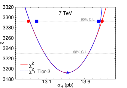
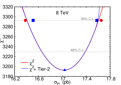
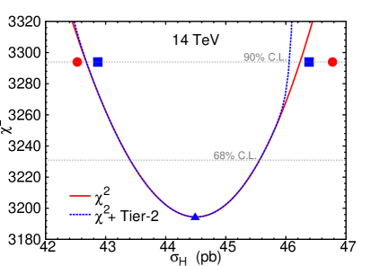
The red solid curves, which are approximately parabolic, show $\chi^{2}$ versus $\sigma_{H}$; the blue dashed curves are for $\chi^{2}+$tier-2 penalty versus $\sigma_{H}$. The two curves are almost identical over much of the range plotted. They only begin to diverge at large values of $|\sigma_{H}-\sigma_{H}(a_{0})|$, where one or more experimental data sets can no longer be satisfactorily fit, resulting in a large tier-2 penalty. The blue triangles on the curves in Fig. 1 are the central values of $\sigma_{H}$, and the blue boxes are the upper and lower $90\%$ C.L. limits, calculated in the Hessian method and listed in Table 2. The red circles correspond to the same quantities, also calculated in the Hessian method, but without including the tier-2 penalties. They are plotted at the vertical value of $\Delta\chi^{2}=T^{2}=100$, and are to be compared to the curves calculated by the LM method.

By comparing the red solid curves and the red circles, and noting the parabolic nature of the red solid curves, we note that the quadratic approximation works well for $\sigma_{H}(gg\to H)$, up to the tolerance bounds of $T^{2}=100$. Also, the LM and Hessian methods, without including the tier-2 penalty, give comparable estimates of the PDF errors on $\sigma_{H}$. (The two error estimates without including the tier-2 penalty do differ somewhat more at 14 TeV.) After including the tier-2 penalties in both the LM and Hessian methods, shown by the blue dashed curves and blue boxes, we find that the error predictions become more asymmetric. However, the differences in the error estimates by the four methods shown in Fig. 1 are still considerably smaller than the error estimates themselves. Table 3 gives the numerical values of the central predictions and asymmetric errors for $\sigma_{H}$, obtained from the LM method, with the tier-2 penalties included. Comparing Tables 2 and 3, we find that the PDF uncertainty estimates predicted by both methods are similar.

A technical detail in both our LM and Hessian calculations concerns the normalizations of the fixed target DIS experiments BCDMS, CDHSW and CCFR. These experiments have large numbers of data points, and rather small quoted normalization uncertainties ($3\,$%, $1\,$%, and $2.6\,$% respectively). We found in previous CTEQ global analyses, e.g., in calculating the uncertainty of $W^{\pm}$ or $Z^{0}$ production cross sections at the Tevatron, that allowing these normalizations to vary beyond their published standard deviations could produce fits with fairly small $\chi^{2}$, for quite large deviations of $\sigma_{W}$ or $\sigma_{Z}$. But these fits were not acceptable because they required large shifts in the normalizations of the DIS data Stump:2001gu . For this reason we have chosen both in the past and in the current Higgs study (including the published CT10 Hessian set) to fix the normalizations of these three experiments at their best fit values.

LHC	7 TeV	8 TeV	14 TeV
$\sigma_{H}(gg\to H)$ (pb) with $90\%$ C.L. errors	$13.4^{+3.2\%}_{-3.7\%}$	$17.0^{+3.2\%}_{-3.7\%}$	$44.5^{+3.5\%}_{-4.1\%}$
with 68% C.L. errors	$13.4^{+2.0\%}_{-2.2\%}$	$17.0^{+2.0\%}_{-2.3\%}$	$44.5^{+2.2\%}_{-2.4\%}$

Table 3: Higgs boson production cross sections (in pb unit) via gluon fusion channel at the LHC, with 7, 8 and 14 TeV center-of-mass energy. The PDF uncertainties at the $90\%$ C.L. and $68\%$ C.L. were calculated by the Lagrange multiplier method in the CT10H analysis with fixed $\alpha_{s}(M_{Z})=0.118$. The uncertainties are expressed as the percentage of the central value.

III.3 The LM calculation of the combined PDF$+\alpha_{s}$ uncertainty of $\sigma_{H}$

In the previous subsection, we presented results using the LM method, while treating $\alpha_{s}(M_{Z})$ as a fixed parameter, equal to the current world-average value. We now consider the combined PDF and $\alpha_{s}(M_{Z})$ effects in the LM method, by including the world-average constraints on $\alpha_{s}(M_{Z})$ directly in the $\chi^{2}$ function, using Eq. (8) and treating $\alpha_{s}(M_{Z})$ as an additional fitting parameter. In practice, we select $\alpha_{s}(M_{Z})$ from a set of discrete values and repeat a LM scan of $\chi^{2}$ for each selected $\alpha_{s}(M_{Z})$; that determines the constrained $\chi^{2}(\overline{a})$ versus $\sigma_{H}(\overline{a})$ in a range of $\alpha_{s}(M_{Z})$. (The term with $\kappa=100$ introduced in Eq. (8) to specify the world-average constraints on $\alpha_{s}(M_{Z})$ is now included as a part of $\chi^{2}$.) We perform the calculations for a series of values of $\alpha_{s}(M_{Z})$. Then, we have $\chi^{2}$ as a function of $(\alpha_{s}(M_{Z}),\sigma_{H})$, and we can trace out contours of $\chi^{2}$ in the $(\alpha_{s},\sigma_{H})$ plane.

Figure 2: Contour plots of $\chi^{2}(\overline{a})$ in the $(\alpha_{s},\sigma_{H})$ plane, for $\sigma_{H}$ (in pb unit) at the LHC, with 7, 8 and 14 TeV. The thick black outer and inner contours are at $\Delta\chi^{2}=100$ and $100/(1.645)^{2}$, respectively, for the $90\%$ C.L. and $68\%$ C.L.. The thin colored contours are at intervals in $\chi^{2}$ of 10.

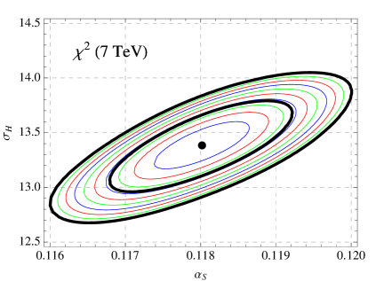
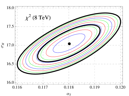
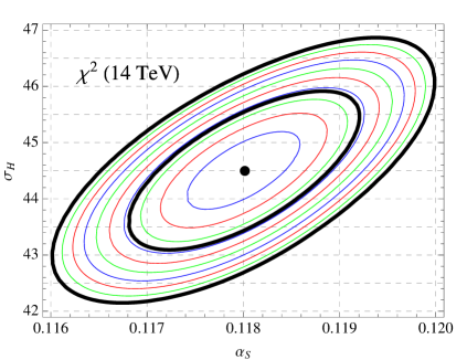
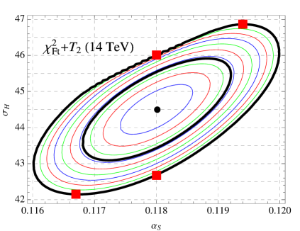
Figure 2 shows the contour plots of $\chi^{2}(\overline{a})$ in the $(\alpha_{s},\sigma_{H})$ plane, for $\sigma_{H}$ at the LHC with $\sqrt{s}=$ 7, 8 and 14 TeV. A contour here is the locus of points in the $(\alpha_{s},\sigma_{H})$ plane along which the constrained minimum of $\chi^{2}$ is constant. Note that we have not included the tier-2 penalty in the calculation of $\chi^{2}$ for Fig. 2. We see from these figures that the values of $\sigma_{H}$ and $\alpha_{s}(M_{Z})$ are strongly correlated, as expected, given the strong dependence of the $gg$ fusion cross section on $\alpha_{s}(M_{Z})$ at NNLO. Larger values of $\alpha_{s}(M_{Z})$ correspond to larger values of $\sigma_{H}$ for the same goodness-of-fit to the global data, even though there is a partially compensating decrease of the $gg$ luminosity.

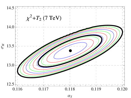
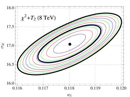
The contour with $\chi^{2}-\chi_{0}^{2}=T^{2}$ is particularly interesting, because it represents our estimate for the correlated uncertainties of $\alpha_{s}$ and $\sigma_{H}$ at the $90\%$ C.L.. This contour gives $\alpha_{s}(M_{Z})=0.118\pm 0.002$, as we expected from the discussion in Section II. By finding the extreme values of $\sigma_{H}$ along the contour, we obtain the combined PDF $+\alpha_{s}$ errors on the Higgs cross section, which are displayed inTable 4. Similar results at the $68\%$ C.L. are also shown in both Fig. 2 and Table 4.

LHC	7 TeV	8 TeV	14 TeV
$\sigma_{H}(gg\to H)$ (pb) with $90\%$ C.L. errors	$13.4^{+4.8\%}_{-5.0\%}$	$17.0^{+4.6\%}_{-4.6\%}$	$44.5^{+5.2\%}_{-5.2\%}$
with 68% C.L. errors	$13.4^{+2.9\%}_{-3.2\%}$	$17.0^{+2.8\%}_{-2.9\%}$	$44.5^{+3.4\%}_{-3.2\%}$

Table 4: Higgs boson production cross sections via gluon fusion channel at the LHC, with 7, 8 and 14 TeV. The combined PDF and $\alpha_{s}$ uncertainties at the $90\%$ C.L. have been calculated by the Lagrange multiplier method in the CT10H analysis. The errors are expressed as the percentage of the central value.

Figure 2 shows the minimum global $\chi^{2}$ value, without tier-2 penalty, as a function of $(\alpha_{s},\sigma_{H})$. However, we have argued previously that including the tier-2 penalty with the $\chi^{2}$ function is a better indicator of goodness-of-fit. Therefore, in Fig. 3, we present contour plots of $\chi^{2}+$ tier-2 penalty in the $(\alpha_{s},\sigma_{H})$ plane, for $\sigma_{H}$ at the LHC with $\sqrt{s}=$ 7, 8 and 14 TeV. The tier-2 penalty has a small effect for 7 and 8 TeV. The effect is larger for 14 TeV, especially for $\sigma_{H}\gg\sigma_{H}(a_{0})$. The tier-2 penalty does reduce the uncertainty of the prediction of $\sigma_{H}$: the area enclosed by any contour is smaller in Fig. 3. However, the reduction of uncertainty is fairly small. In addition, the change in the maximum and minimum values of $\sigma_{H}$ along the $\Delta\chi^{2}=100$ contour is negligible, even for $\sqrt{s}=14$ TeV.

Figure 3: Contour plots of $\chi^{2}+\mbox{tier-2}$ ($T_{2}$) in the $(\alpha_{s},\sigma_{H})$ plane, for $\sigma_{H}$ (in pb unit) at the LHC, with 7, 8 and 14 TeV. The thick black outer and inner contours are at $\Delta\chi^{2}=100$ and $100/(1.645)^{2}$, respectively, for the $90\%$ C.L. and $68\%$ C.L.. The thin colored contours are at intervals in $\chi^{2}$ of 10. The fits that give minimum and maximum $\sigma_{H}$ are indicated by the red square symbols, with $\alpha_{s}(M_{Z})=0.1167$, $0.118$ or $0.1194$. (See the text in Sec. IV.C for its details.)

III.4 Comparisons of LM and Hessian uncertainties

From Tables 3 and 4 (LM method) and Table 2 (Hessian method) we can compare the PDF-only uncertainties, as well as the combined PDF + $\alpha_{s}$ uncertainties, on the $gg\to H$ cross section computed by the two methods. The PDF-only uncertainties are for $\alpha_{s}(M_{Z})=0.118$. The central values of $\sigma_{H}(\,7\ {\rm TeV})$, $\sigma_{H}(\,8\ {\rm TeV})$ and $\sigma_{H}(\,14\ {\rm TeV})$ are identical in both calculations by definition, so we can use the percent error to compare the uncertainties. Both methods give asymmetric errors, which are compared in Table 5.

	90% C.L.			68% C.L.
Method	7 TeV	8 TeV	14 TeV	7 TeV	8 TeV	14 TeV
LM (PDF-only)	+3.2/-3.7	+3.2/-3.7	+3.5/-4.1	+2.0/-2.2	+2.0/-2.3	+2.2/-2.4
Hessian (PDF-only)	+3.0/-3.0	+3.2/-3.1	+4.3/-3.6	+1.8/-1.8	+1.9/-1.9	+2.6/-2.2
LM (PDF + $\alpha_{s}$)	+4.8/-5.0	+4.6/-4.6	+5.2/-5.2	+2.9/-3.2	+2.8/-2.9	+3.4/-3.2
Hessian (PDF + $\alpha_{s})$	+4.7/-4.6	+4.8/-4.7	+5.4/-5.0	+2.9/-2.8	+2.9/-2.8	+3.3/-3.0

Table 5: Uncertainties of $\sigma_{H}(gg\to H)$ computed by the LM method and by the Hessian method, with tier-2 penalty included. The $90\%$ and $68\%$ C.L. errors are given as percentage of the central value, and the PDF-only uncertainties are for $\alpha_{s}=0.118$.

From Table 5 we see that the PDF-only uncertainties (for $\alpha_{s}(M_{Z})=0.118$) are fairly similar in both methods of calculation. The LM method tends to be slightly more asymmetric, with larger negative uncertainties, due to the slight non-quadratic behavior of the $\chi^{2}$ function. The case of $\sqrt{s}=14$ TeV is interesting because the direction of the asymmetry in the errors is opposite between the LM and Hessian methods. However, for all collider energies, the difference in the error estimates between the two methods are considerably smaller than the estimates themselves, and also smaller than the general theoretical uncertainty in defining the $90\%$ C.L. errors (the choice of tolerance $T$, for example.)

For the combined PDF + $\alpha_{s}$ errors, the agreement between the two methods of calculation is also good. In the LM method, the errors tend to be less asymmetric when the $\alpha_{s}$ uncertainty is included, which brings the estimates from the two methods into even better agreement. For example, for $\sqrt{s}=8$ TeV and $\sqrt{s}=14$ TeV the difference between the two PDF + $\alpha_{s}$ error estimates is less than $5\%$ of the error estimates themselves. This C.L.early shows that the Hessian method of combining the PDF and the $\alpha_{s}$ errors in quadrature is valid, and that the Hessian method gives a reliable error estimate in the case of the $gg\to H$ cross section.

The fact that the Hessian and Lagrange multiplier estimates are in good agreement for the Higgs boson cross section is because the $\chi^{2}$ dependence on the fitting parameters $\{a\}$ is mostly quadratic in the relevant tolerance range, and that $\sigma_{H}$ is predominantly a linear function of the parameters in the same range. Furthermore, the tier-2 penalty does not have a very large effect here, only turning on near the edge of the uncertainty range. Thus, the error estimates from the Hessian method are in good, though not perfect, agreement with those from the LM method. In addition, this explains why the Hessian method of adding the $\alpha_{s}$ uncertainties in quadrature works quite well, and why the prescription for obtaining the $68\%$ C.L. errors from the $90\%$ C.L. errors is reasonable.

We must emphasize here that these conC.L.usions apply only to the $gg\to H$ cross section with $M_{H}=125$ GeV. In particular, the assumption that the observable $(\sigma_{H})$ depends linearly on the fitting parameters $\{a\}$ over the relevant range might not be true for other observables. Even in the case of the Higgs boson cross section from gluon fusion, one might have expected larger nonlinear effects, since the cross section depends strongly on both the gluon PDF $g(x,Q)$ and the value of $\alpha_{s}$. For other observables, which may be more sensitive to other aspects of the PDFs, the nonlinear effects may be greater. This may especially be true if the observable is strongly correlated with a single experimental data set in the global analysis, which would lead to a large contribution from the tier-2 term. In this case the LM and Hessian methods would give larger and more significant differences, with the LM method giving the more reliable error estimate. Thus, the LM method provides an important alternative to the simpler Hessian method.

In conclusion, for $\sigma_{H}$ the Hessian and LM methods give consistent results; and the tier-2 penalties have small effects. We find this somewhat surprising for the following reasons: (i) We use a rather large tolerance value, $T\lesssim 10$, which one might expect to allow nonlinearities in the dependences of $\chi^{2}(a)$ and $\sigma_{H}(a)$ on $\left\{a\right\}$. Meanwhile, the Hessian method is based on a linear error analysis. Nevertheless, the final results are consistent with the LM method, which does not rely on linearity. (ii) The fact that the uncertainties are asymmetric shows that nonlinearities do exist; but again the Hessian treatment of the asymmetric errors is satisfactory. (iii) Simply combining PDF error and $\alpha_{s}$ error in quadrature in the Hessian method, gives results similar to the full $\sigma_{H}$ and $\alpha_{s}$ correlated uncertainties obtained in the LM method.

Are the above results surprising or not? We would not know whether the Hessian method is reasonable, without completing the LM calculations. This is important to know, because the Hessian method—using the LHAPDF library of error PDFs—is the only method available for most studies of PDF uncertainty. Furthermore, the LM calculations are interesting for another reason. They allow the construction of the contour plots, which demonstrate very dramatically the correlations between $\sigma_{H}$ and $\alpha_{s}$ uncertainties.

IV Correlations between $\sigma_{H}$ and PDFs

The Hessian and LM calculations are each better suited for elucidating different aspects of how the PDFs influence the uncertainty in the Higgs boson cross section. In this section we examine some of these details for the two methods in turn.

IV.1 Error Sets and Correlation Cosines in the Hessian Method

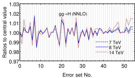
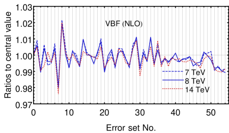
The error sets that are obtained in the Hessian method can be used to compare the sensitivity of different observables to the various PDF parameters Nadolsky:2008zw . In Fig. 4 we plot the ratios of the predictions from each of the error sets to the best-fit set, for the Higgs boson cross section at the LHC, in both the gluon fusion and vector boson fusion (VBF) subprocesses. In this study, we use a slightly enhanced set of PDF parameters, with two additional eigenvectors in the PDF parameter space, as compared to the CT10 NNLO PDFs. As usual, these error sets were obtained after including the tier-2 penalty in the global analysis. The VBF cross sections were calculated up to NLO using the VBFNLO-2.6.1 code vbfnlo , with both the renormalization and the factorization scales set to $\mu=M_{H}=125\ {\rm GeV}$, and with all the other default settings, including a minimal invariant mass cut of $600\ {\rm GeV}$ for the two tagging jets.

The results for the $gg$ fusion and VBF channels are shown in the upper and lower panels of Fig. 4. The dashed, solid, and dotted lines are for the LHC energy at 7, 8, and 14 TeV, respectively. It is interesting to note that the relative importance of the major error sets (i.e., the eigenvectors in the PDF parameter space) is roughly independent of the collision energy. In the case of the $gg\to H$ cross section, we see that the PDF uncertainties at all three energies are dominated by a few eigenvectors, which are associated with the variations of the gluon PDF. Furthermore, the values for the $gg$ fusion and for the VBF subprocesses in these figures tend to be opposite in sign (at least for the first few error sets, with largest eigenvalues), indicating the anti-correlation of the two subprocesses. Namely, the error sets that increase the $gg\to H$ cross section will decrease the VBF cross section, and vice versa. Moreover, the PDF induced errors in the ratios of $gg\to H$ cross sections at different LHC energies are expected to be small, about $2\%$ with its center value around 3.3 in the ratio of 14 TeV to 7 TeV predictions, evaluated at the 90% C.L.. A similar result holds for the VBF process, with its center value around 4.4.

Figure 4: Ratio of the prediction of the Higgs boson cross section from each error set to that from the central set. The results for the $gg$ fusion and VBF channels are shown in the upper and lower panels. The dashed, solid, and dotted lines are for the LHC energy at 7, 8, and 14 TeV, respectively.

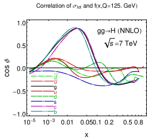
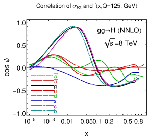
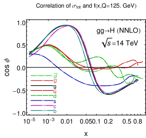
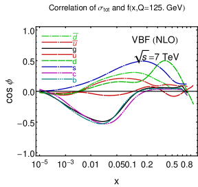
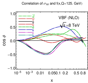
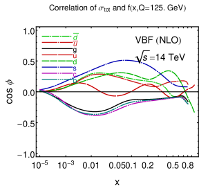
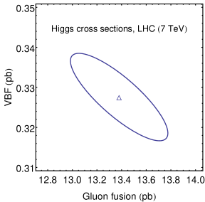
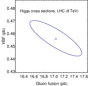
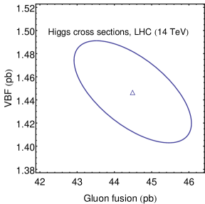
In the Hessian approach, assuming quadratic approximation, we can also study the direction of the gradient of the Higgs boson cross section in the PDF parameter space Pumplin:2001ct ; Nadolsky:2008zw ; Nadolsky:2001yg . Figure 5 shows the correlation between $\sigma_{H}$ and the PDFs of different flavors, as a function of the parton momentum fraction $x$. The correlation of two observables is measured by the cosine of the angle between the gradient directions of the two observables in the PDF parameter space Nadolsky:2008zw . From Fig. 5 we can see a strong correlation between the $gg\to H$ cross section and the gluon PDF at $x\sim 0.01$, as expected. The charm and bottom PDFs track the gluon PDF in these plots, since they arise through gluon splitting. Figure 6 shows a similar, but weaker, correlation with the gluon PDF for the VBF process. The correlations between the gluon PDF and the two different subprocesses are opposite in sign, consistent with the error PDF plots in Fig. 4. We can see this moderate anti-correlation directly in the 90% C.L. correlation ellipse of the two Higgs boson production subprocesses, as shown in Fig. 7.

Figure 5: Correlation cosine between the $gg\to H$ cross sections and the PDFs at $Q=125\ {\rm GeV}$ as functions of $x$, at the LHC, with 7, 8, and 14 TeV.

Figure 6: Correlation cosine between the VBF component of $\sigma_{H}$ and the PDFs at $Q=125\ {\rm GeV}$ as functions of $x$, at the LHC, with 7, 8, and 14 TeV.

Figure 7: The $90\%$ tolerance ellipse of $(\sigma_{H})_{gg}$ and $(\sigma_{H})_{\rm VBF}$ at the LHC, with 7, 8, and 14 TeV.

IV.2 Correlations between data sets and $\sigma_{H}$ in the LM method

Consistent with the error analysis in the LM method, we can learn more about the impact of data on the PDF analysis by calculating the correlations between individual data sets and the PDFs with constrained values of $\sigma_{H}$. In this section, we identity the experimental data sets that correlate most strongly with the constrained value of $\sigma_{H}$ (via the $gg$ channel) from the Lagrange multiplier calculations.

In a LM calculation, the constrained value of $\sigma_{H}$ can be pushed to a larger or smaller value, as compared to its central value $\sigma_{H}(a_{0})$ (corresponding to $\lambda=0$), by changing the value of $\lambda$; cf. Eq. (6). We now examine the degree to which the change in $\sigma_{H}$ causes a specific data set to agree less well with the theory prediction than for $\lambda=0$. We need a measure of goodness-of-fit to address the question. We could compare variations of the figures-of-merit $\chi_{e}^{2}$ for each experimental data set in the scan over $\lambda$, but would find such comparison inscrutable because of different sizes $N_{pt}$ of the experimental data sets and, consequently, their incompatible $\chi^{2}_{e}(N_{pt})$ distributions. Instead, we make use of an ‘equivalent Gaussian variable” $S$ Dulat:2013hea , introduced originally as a part of the tier-2 penalty Lai:2010vv .

For each particular data set assumed to obey a chi-squared probability distribution, we map the $\chi^{2}_{e}({a},N_{\mathrm{p}t})$ value of the data set onto a respective variable $S_{e}$, which has the same cumulative probability, but obeys a Gaussian distribution with unit standard deviation. A more detailed definition of $S_{e}$ and its relation to the $\chi^{2}$-probability distribution function can be found in Ref. Dulat:2013hea . A value of $S_{e}$ in the range of $-1$ to $1$ indicates a good agreement (at the $68\%$ C.L.) between data and theory, analogous to $\chi_{e}^{2}\approx N_{\mathrm{p}t}$, in the case of large $N_{\mathrm{p}t}$. $S_{e}$ much larger than $+2$ indicates a poor fit, analogous to $\chi_{e}^{2}\gg N_{\mathrm{p}t}$. $S_{e}$ much less than $-2$ indicates an unexpectedly good fit, much better than one would expect from normal statistical analysis; i.e., they have anomalously small residuals, presumably because the true experimental errors are smaller than the published values.

Something important is gained by this mapping. The statistical meaning of the value of $\chi^{2}_{e}/N_{\mathrm{p}t}$ depends on $N_{\mathrm{p}t}$; but the mapping to $S_{e}$ removes this complication. For example, the confidence levels on $S_{e}$ in the previous paragraph are independent of $N_{pt}$, so in Figure 8 we plot $S_{e}$ to compare sensitivities of the data sets to the changes in the PDFs that also change the prediction for $\sigma_{H}$. A similar figure showing $\chi^{2}/N_{\mathrm{p}t}$ would be far less informative: the meaning of each curve would depend on $N_{\mathrm{p}t}$, which varies from 8 to 579 among the 33 data sets (cf. Table 1).

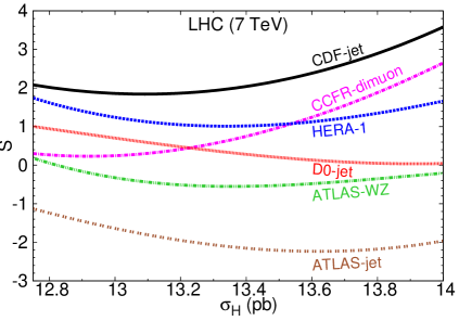
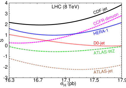
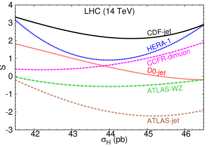
In Fig. 8, the values of $S$ are shown versus the constrained values of $\sigma_{H}$ at the LHC with 7, 8, and 14 TeV for the four experimental data sets with ID numbers 126, 159, 504 and 514 (cf. Table 1). These are the experiments whose $S$ values show strong correlation to the constrained values of $\sigma_{H}$, at all three energies of the LHC. We also plot the values of $S$ for the two LHC data sets, ID numbers 268 and 535. As we push $\sigma_{H}$ away from its central value $\sigma_{H}(a_{0})$, we see that $S$ increases substantially for some data sets, corresponding to a worse agreement between data and theory. The upper four experiments shown in Fig. 8 are sensitive to the constrained theoretical value of $\sigma_{H}$, because the increase in $S$ signals a decrease in likelihood for that value of $\sigma_{H}$.

It is not surprising that the $S$ dependence indicates that the inclusive high-$p_{T}$ jet production measurements at the Tevatron by the CDF (ID number 504) and D0 (ID number 514) Collaborations are strongly correlated to the constrained value of $\sigma_{H}$ at the LHC, because these are the experimental data that are sensitive to the gluon PDF. Similarly, the marked variation of $S$ for the combined HERA Run 1 data set (ID number 159) is understood, because it is well known that the HERA data provide important constraints on determining the gluon PDF. The pattern of sensitivity to $\sigma_{H}$ is similar for all three LHC energies, although we note that the combined HERA Run 1 data set increases in importance as the collider energy increases and smaller $x$ values for the gluon are sampled. The sensitivity of $S$ for the CCFR neutrino dimuon data Goncharov:2001qe (ID number 126) is less obvious. After a careful examination, we find that in the CT10H PDF sets, when the gluon PDF increases to push up the constrained value of $\sigma_{H}$, the strange PDF decreases at a $Q$ value around 3 GeV and $x$ value of order $10^{-2}$, so as to strongly reduce the predictions compared to the CCFR dimuon data in that kinematic region. This is mainly due to the momentum sum rule imposed on the parton distribution functions.

A final observation is that the $S$ values for the two LHC data sets, the combined ATLAS $W^{\pm}$ and $Z$ data (ID number 268) and the ATLAS inclusive jet data (ID number 535), are all smaller than zero within the $90\%$ C.L. range of $\sigma_{H}$, at all three energies of the LHC, as seen in Fig. 8. This indicates that these data are easily fit in the global analysis, and hence, they do not play a significant role in constraining the Higgs boson cross section at the LHC, as predicted by the CT10H PDF sets. Needless to say, these conclusions could change in the future with more precise data from the LHC.

Figure 8: The equivalent Gaussian variable $S$ versus $\sigma_{H}$ (in pb unit) at the LHC, with 7, 8 and 14 TeV. The labels CDF, D0, HERA-1, CCFR-dimuon, ATLAS_WZ, and ATLAS_jet correspond to the experiment ID numbers 504, 514, 159, 126, 268, and 535, respectively, given in Table 1.

IV.3 Extreme PDFs from the Lagrange multiplier fits

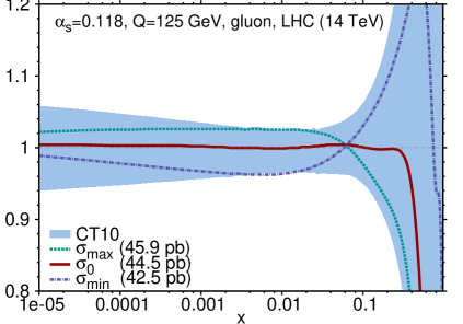
To facilitate the study of PDF uncertainties in the prediction of $gg\to H$ total cross section, we make available on LHAPDF lhapdf a few PDFs implementing the findings of our CT10H Lagrange multiplier study. The CT10H ensemble consists of the central set, two sets for determination of the 90% C.L. PDF uncertainty on $\sigma_{H}$ at 14 TeV with a fixed $\alpha_{s}(M_{Z})=0.118$ (corresponding to the red square symbols in Fig. 3), and two other sets to determine the 90% C.L. extremes on $\sigma_{H}$ from the combined PDF+$\alpha_{s}$ analysis at 14 TeV. In the second pair of PDF sets, the upper and lower uncertainty limits on $\sigma_{H}$ correspond to $\alpha_{s}(M_{Z})=0.1194$ and $0.1167$, respectively. The CT10 and CT10H central sets are entirely compatible and can be used interchangeably. While the extreme sets are derived to predict the PDF-induced errors in $\sigma_{H}$ at the LHC with $14\,\mathrm{TeV}$, they also reproduce the corresponding errors at 7 and 8 TeV to sufficient accuracy.

Figure 9 compares the gluon distributions from CT10H to the CT10 NNLO uncertainty band, with $\alpha_{s}=0.118$, at the $90\%$ C.L.. One sees that the CT10H uncertainty is practically the same as the CT10 NNLO range for $0.002\lesssim x\lesssim 0.03\,$, which is the region dominating the Higgs boson total cross section via gluon fusion channel at the LHC. In this $x$ region, the pair of CT10H PDFs significantly reduces the computational burden in estimating the uncertainties, compared to CT10. The CT10H sets underestimate the PDF-induced uncertainty in predicting the kinematical distributions of the Higgs boson sensitive to the gluon PDF with $x$ less than $10^{-4}$ or above $0.05$, where the full CT10 PDF ensemble is needed. The CT10H sets can be also used to estimate the PDF uncertainty in processes that are strongly correlated with $gg\rightarrow H$ production. For instance, the CT10H extreme sets predict more than a half of the CT10 PDF-induced error in Higgs boson production cross section via vector boson fusion, because of the moderate anti-correlation of the $gg\to H$ and VBF processes discussed in Sec. IV.A, and about a half of the CT10 error in the associated $t{\bar{t}}H$ production.

Figure 9: CT10H gluon PDFs at the momentum scale 125 GeV, compared to the CT10 error band, at the $90\%$ C.L.. These CT10H fits give the central prediction ($\sigma_{0}$), and the minimum ($\sigma_{min}$) and maximum ($\sigma_{max}$) predictions obtained using the Lagrange multiplier method, for $\sigma_{H}$ at the LHC with 14 TeV, as listed in Table 3. Also, $\alpha_{s}(M_{Z})=0.118$.

Our general-purpose PDFs at this time remain CT10 NNLO PDFs. The CT10H extremes should only be used for calculations of uncertainties specifically related to Higgs boson production at central rapidities at the LHC. In the future, when additional LHC data become available, the CTEQ-TEA collaboration will construct a new generation of general PDFs including that data in the analysis.

V Conclusions

Accurate predictions for the rates of Higgs boson production are crucial for precision tests of the Higgs mechanism. Studying the production rates and decay branching ratios of the Higgs boson can potentially discriminate between models of electroweak symmetry breaking, and the goal is to measure them with an accuracy better than $10\%$ Dittmaier:2011ti ; SnowmassHiggs2013 .

In the dominant gluon-gluon fusion channel, the two key contributions to the error in the Higgs boson production rate are the uncertainties of the PDFs and the QCD coupling $\alpha_{s}$. In this paper, we addressed the estimation of the PDF uncertainty, as well as the combined PDF+$\alpha_{s}$ uncertainty, for the Higgs boson production cross section at the LHC. In general, various methods for estimation of the PDF uncertainty may yield somewhat different results, with potential phenomenological implications. For example, nonlinearities in the log-likelihood function $\chi^{2}$ employed in the PDF fits could produce differences between the error estimates obtained by different methods of the analysis. Thus, it is important to determine the magnitude of the difference.

In the present work, we have used the CT10 NNLO global analysis (with minor updates), which we call CT10H NNLO, to investigate this issue. We compared two standard methods for performing the error analysis: the Hessian method, which utilizes an eigenvector decomposition of the PDF parameter space; and the Lagrange multiplier method, which utilizes constrained global fits of the PDFs. A set of eigenvector PDFs has been previously distributed by the CT10 NNLO global analysis ct10nnlo to compute the PDF uncertainty for any experimental observable in the Hessian method. By comparing the results from this method to those from the LM method, which makes fewer assumptions about the functional dependence of $\chi^{2}$ on the PDF parameters, we have checked the reliability of the Hessian result in the particular case of the production of SM Higgs boson, with a 125 GeV mass, via the gluon-gluon fusion channel.

Our main conclusion from this analysis is that the two methods give quite similar predictions for the PDF uncertainty on the $gg\to H$ cross section, thus supporting previous results that relied exclusively on the Hessian method. For the pure PDF uncertainty, both methods give relative errors of about $\pm 3$ to $\pm 4\%$ at the 90% C.L. for the different energies, with small differences between the methods. For the combined PDF+$\alpha_{s}$ error, the two methods agree even better, validating the prescription of adding the Hessian PDF errors and the $\alpha_{s}$ errors (obtained from the $\alpha_{s}$ series of PDFs) in quadrature. For example, the combined uncertainty at $\sqrt{s}=14$ TeV was found to be $\pm 5.2$% in the LM method and $+5.4/-5.0$% in the Hessian method at the 90% C.L.. Both methods in general yield a mild asymmetry in the errors. The differences between the two methods are certainly less than other theoretical uncertainties, such as in the choice of tolerance used to define the 90% C.L.. We have tried several nonperturbative parametrization forms for the CT10H PDFs, but found little change in the predictions and no change in our overall conclusions.

The agreement between the two methods is not trivial, given the variety of involved factors. It can be traced to the fact that the $\chi^{2}$ dependence on $\sigma_{H}$ is close to parabolic and is not strongly affected by constraints from individual experiments (i.e., by the tier-2 penalty), within the tolerance range. In addition, the approximately quadratic behavior in $\chi^{2}$ implies that the method for obtaining a 68% C.L. interval from the 90% C.L. interval, by dividing by 1.645, is appropriate. We emphasize that these fortunate features of the $\chi^{2}$ function may not hold for other processes that are sensitive to other PDF flavors or to the gluon PDF in a different range of $x$. A full comparison of two methods would need to be repeated to check if they agree for any other observable. Furthermore, if the observable is strongly correlated with a single experimental data set in the global analysis, which would lead to a large contribution from the tier-2 penalty, the LM and Hessian methods would yield different predictions, with the LM method giving a more reliable error estimate.

In this paper we also presented some details of the uncertainty analysis that were obtained with the two methods. Using the Hessian method, we showed that the PDF dependence produces a strong anti-correlation between the prediction for the rate of Higgs boson production through gluon-gluon fusion and that for vector boson fusion, at all three collider energies. Using the LM method, we investigated the correlation between the value of $\alpha_{s}(M_{Z})$ and the Higgs boson cross section in gluon-gluon fusion, as displayed in the contour plots of Figs. 2 and 3. We also checked the impact of individual experimental data sets on the prediction of the Higgs boson cross section. As expected, the data sets that constrain $\sigma_{H}$ most strongly are the Tevatron jet data and the HERA Run 1 DIS data, which are most sensitive to the gluon PDF. Agreement with the HERA data set, in particular, is strongly sensitive to variations in the Higgs boson cross section at 14 TeV.

From the LM scan we have obtained a pair of PDF sets that are sufficient to determine the two uncertainty extremes in the $gg\to H$ cross section at $\sqrt{s}=14$ TeV, with a fixed $\alpha_{s}(M_{Z})=0.118$. Similarly, we have obtained a pair of PDF sets that determine the uncertainty extremes from the combined PDF+$\alpha_{s}$ analysis at 14 TeV. In this second pair of PDF sets, the one that gives the upper uncertainty limit on $\sigma_{H}$ corresponds to a value of $\alpha_{s}(M_{Z})=0.1194$, while the one that gives the lower uncertainty limit corresponds to a value of $\alpha_{s}(M_{Z})=0.1167$. Although the equivalent error sets for other energies will be slightly different, we have checked that both of these pairs of PDF sets reproduce the corresponding errors found at 7 and 8 TeV to reasonable accuracy. These PDF sets will simplify the experimental analysis on the uncertainty in the Higgs boson total cross section through gluon-gluon fusion, compared to the standard Hessian method analysis, as only two PDF error sets are needed to compute the PDF error. These PDF sets are to be included in the LHAPDF library lhapdf and also be made available via the internet website ct10web which hosts all CT10 PDFs.

Appendix 1. Analytic study of $\alpha_{s}$ and $\sigma_{H}$ uncertainties

In the formula for $\chi^{2}$ with the $\kappa$-penalty, given by Eqs. (1) and (8), we can consider the fit parameters as functions of $\sigma_{H}$ and $\alpha_{s}\equiv\alpha_{s}(M_{Z})$, (i.e., $a_{i}\equiv a_{i}(\sigma_{H},\alpha_{s})$), implicitly via the Lagrange multiplier calculation. In this way we can treat $\chi^{2}$ as a function of $\sigma_{H}$ and $\alpha_{s}$:

$$\chi^{2}(\sigma_{H},\alpha_{s}) \equiv \chi^{2}(a_{i}(\sigma_{H},\alpha_{s}),\alpha_{s})$$ (11)

$$= \chi_{0}^{2}(\sigma_{H},\alpha_{s})+\kappa\left(\frac{\alpha_{s}-\bar{\alpha}}{\delta\bar{\alpha}}\right)^{2}$$

where $\chi_{0}^{2}(\sigma_{H},\alpha_{s})$ is the $\chi^{2}$ value for $\kappa=0$. In this appendix, we will consider this formula in the quadratic approximation in order to understand the interplay of the PDF and $\alpha_{s}$ contributions to the uncertainty on the Higgs boson cross section. Consequently, we shall relate these results to the combined uncertainty obtained in the Hessian method.

For $\kappa=0$, and working in the quadratic approximation, we can write

$$\chi_{0}^{2}(\sigma_{H},\alpha_{s}) \approx \chi_{0}^{2}(\sigma^{0}_{H},\alpha^{0}_{S})+M_{11}(\sigma_{H}-\sigma_{H}^{0})^{2}+M_{22}(\alpha_{s}-\alpha_{s}^{0})^{2}$$ (12)

$$\qquad\qquad\quad+\,2M_{12}(\sigma_{H}-\sigma_{H}^{0})(\alpha_{s}-\alpha_{s}^{0})\ ,$$

where $\sigma_{H}^{0}$ and $\alpha_{s}^{0}$ are the best-fit values for $\kappa=0$, and

$$M_{11} = \frac{1}{2}\frac{\partial^{2}\chi_{0}^{2}}{\partial{\sigma_{H}}^{2}}\Bigg{|}_{\sigma_{H}^{0},\alpha_{s}^{0}}\,$$

$$M_{22} = \frac{1}{2}\frac{\partial^{2}\chi_{0}^{2}}{\partial{\alpha_{s}}^{2}}\Bigg{|}_{\sigma_{H}^{0},\alpha_{s}^{0}}\,$$ (13)

$$M_{12} = \frac{1}{2}\frac{\partial^{2}\chi_{0}^{2}}{\partial\sigma_{H}\partial\alpha_{s}}\Bigg{|}_{\sigma_{H}^{0},\alpha_{s}^{0}}\ .$$

Note that we are treating $\alpha_{s}$ as a fitting parameter. Thus, $\alpha_{s}^{0}\equiv\alpha_{\rm GA}$ is the best-fit value as determined purely by the global analysis (GA) data. From Eq. (12) we can also obtain the 90% confidence level uncertainty on $\alpha_{s}$ coming purely from the global analysis:

$$\delta{\alpha}_{\rm GA} = \frac{T^{2}M_{11}}{D}\ ,$$ (14)

where $T$ is the tolerance level on $\chi^{2}$ used in the global analysis and $D=M_{11}M_{22}-(M_{12})^{2}$ is the determinant of the matrix $M_{ij}$. If we assume that the determination of $\bar{\alpha}$ and $\alpha_{\rm GA}$ are uncorrelated, dependent upon different experimental constraints, we can obtain the total combined uncertainty from

$$\frac{1}{(\delta\alpha_{\rm WA})^{2}} = \frac{1}{(\delta\alpha_{\rm GA})^{2}}+\frac{1}{(\delta\bar{\alpha})^{2}}\ ,$$ (15)

where we have identified the combined uncertainty with the world-average (WA) uncertainty, $\delta\alpha_{\rm WA}$.

For nonzero $\kappa$, we can write

$$\chi^{2}({\sigma}_{H},{\alpha}_{S}) \approx \chi^{2}(\sigma^{\kappa}_{H},\alpha^{\kappa}_{S})+{M}^{\kappa}_{11}({\sigma}_{H}-\sigma^{\kappa}_{H})^{2}+{M}_{22}^{\kappa}({\alpha}_{S}-\alpha^{\kappa}_{S})^{2}$$

$$\qquad\qquad\quad+2\,{M}^{\kappa}_{12}({\sigma}_{H}-\sigma^{\kappa}_{H})({\alpha}_{S}-\alpha^{\kappa}_{S})\ ,$$

where $\sigma^{\kappa}_{H}$ and $\alpha^{\kappa}_{S}$ are the best-fit values with non-zero $\kappa$. Note that all of the parameters in this equation can be obtained as functions of the parameters in Eq. (12), plus $\kappa$ itself. We obtain the relations by plugging Eq. (12) into Eq. (11), and then comparing with Eq. (Appendix 1. Analytic study of $\alpha_{s}$ and $\sigma_{H}$ uncertainties). The quadratic coefficients are

$${M}^{\kappa}_{11} = M_{11}$$

$${M}^{\kappa}_{22} = M_{22}+\kappa/(\delta\bar{\alpha})^{2}$$ (17)

$${M}^{\kappa}_{12} = M_{12}\ .$$

The best-fit values $\sigma^{\kappa}_{H}$, $\alpha^{\kappa}_{S}$, and $\chi^{2}(\sigma_{H}^{\kappa},\alpha_{s}^{\kappa})$ can be expressed in very intuitive forms, if we set $\kappa=T^{2}$ (the tolerance-squared used in the global analysis). Then we find that the best-fit value for $\alpha_{s}$, for non-zero $\kappa$ is

$$\alpha_{s}^{\kappa} = (\delta\alpha_{\rm WA})^{2}\left[\frac{\alpha_{\rm GA}}{(\delta\alpha_{\rm GA})^{2}}+\frac{\bar{\alpha}}{(\delta\bar{\alpha})^{2}}\right]\ .$$ (18)

Note that this is just the average of $\alpha_{\rm GA}$ and $\bar{\alpha}$, weighted by their relative variances. We can identify $\alpha_{s}^{\kappa}\equiv\alpha_{\rm WA}$ as the world-average value, which incorporates all of the experimental constraints on the strong coupling. Similarly, we find

$$\sigma_{H}^{\kappa} = (\delta\alpha_{\rm WA})^{2}\left[\frac{\sigma_{H}(\alpha_{\rm GA})}{(\delta\alpha_{\rm GA})^{2}}+\frac{\sigma_{H}(\bar{\alpha})}{(\delta\bar{\alpha})^{2}}\right]\ ,$$ (19)

where

$$\sigma_{H}(\bar{\alpha})\ \approx\ \sigma_{H}^{0}-(M_{12}/M_{11})(\bar{\alpha}-\alpha_{s}^{0})$$ (20)

is the best-fit result for $\sigma_{H}$ with fixed $\alpha_{s}=\bar{\alpha}$ (in the quadratic approximation), and we have identified $\sigma_{H}^{0}\equiv\sigma_{H}(\alpha_{\rm GA})$. Finally, we obtain a similar result for the minimum value of $\chi^{2}$ at non-zero $\kappa$. We obtain

$$\chi^{2}(\sigma_{H}^{\kappa},\alpha_{s}^{\kappa}) = (\delta\alpha_{\rm WA})^{2}\left[\frac{\chi_{0}^{2}(\sigma_{H}(\alpha_{\rm GA}),\alpha_{\rm GA})}{(\delta\alpha_{\rm GA})^{2}}+\frac{\chi_{0}^{2}(\sigma_{H}(\bar{\alpha}),\bar{\alpha})}{(\delta\bar{\alpha})^{2}}\right]\ ,$$ (21)

where the global minimum with fixed $\alpha_{s}=\bar{\alpha}$ is given by

$$\chi_{0}^{2}(\sigma_{H}(\bar{\alpha}),\bar{\alpha}) \approx \chi_{0}^{2}(\sigma_{H}^{0},\alpha_{s}^{0})+(D/M_{11})(\bar{\alpha}-\alpha_{s}^{0})^{2}\ ,$$ (22)

in the quadratic approximation, and we have identified $\chi_{0}^{2}(\sigma_{H}^{0},\alpha_{s}^{0})\equiv\chi_{0}^{2}(\sigma_{H}(\alpha_{\rm GA}),\alpha_{\rm GA})$.

Next we consider the combined uncertainty in $\sigma_{H}$ obtained from the general $\chi^{2}$ function (11) with a nonzero $\kappa$. In the quadratic approximation, it is straightforward to find the maximum and minimum values of $\sigma_{H}$ that are consistent with a given $\Delta\chi^{2}$. If we require

$$\chi^{2}(\sigma_{H},\alpha_{s})-\chi^{2}(\sigma_{H}^{\kappa},\alpha_{s}^{\kappa})\leq T^{2}\ ,$$ (23)

then we obtain

$$({\sigma}_{H}-\sigma_{H}^{\kappa})^{2} \,\leq\, \left(\frac{{M}^{\kappa}_{22}}{{M}^{\kappa}_{11}{M}^{\kappa}_{22}-({M}^{\kappa}_{12})^{2}}\right)T^{2}$$

$$\,\leq\, \frac{T^{2}}{M_{11}}\ +\ \left(\frac{M_{12}\,\delta\alpha_{\rm WA}}{M_{11}}\right)^{2}\frac{T^{2}}{\kappa}$$

$$\,\leq\, \Sigma_{1}\ +\ \Sigma_{2}\ ,$$

where we have used Eqs. (14) and (15) to simplify the expression. This gives the contribution to the uncertainty in the cross section as the sum of two terms in quadrature, each of which has a specific interpretation. The first term,

$$\Sigma_{1} = \frac{T^{2}}{M_{11}}\ ,$$ (25)

is just the uncertainty-squared in the Higgs boson cross section due to the PDFs at fixed $\alpha_{s}$. We can interpret the second term if we set $\kappa$ equal to our tolerance-squared ($T^{2}/\kappa=1$). Then

$$\Sigma_{2} = \biggl{[}\sigma_{H}(\alpha_{s}+\delta\alpha_{\rm WA})-\sigma_{H}(\alpha_{s})\biggr{]}^{2}\ ,$$ (26)

where we have used the analogous equation to Eq. (20), valid in the quadratic approximation. In the quadratic approximation, the expressions in both Eqs. (25) and (26) do not depend on the exact value of $\alpha_{s}$ used, but it is most reasonable to use the value of $\alpha_{s}=\alpha_{\rm WA}$. Thus, $\Sigma_{1}$ is the uncertainty-squared in the Higgs boson cross section due to the PDFs with the strong coupling fixed at $\alpha_{\rm WA}$, and $\Sigma_{2}$ is just the square of the difference in the best-fit cross sections with the strong coupling fixed at $\alpha_{\rm WA}$ and at $\alpha_{\rm WA}+\delta{\alpha}_{\rm WA}$. This is exactly the standard prescription for obtaining the combined PDF$+\alpha_{s}$ errors used in the Hessian method.

Appendix 2: Benchmark calculations of Higgs boson cross sections

For completeness, we show some benchmark calculations of Higgs boson cross sections at the LHC in the tables below. Table 6 shows a benchmarking comparison of the inclusive cross sections of the SM Higgs boson production at the LHC through the gluon fusion subprocess at the LO, NLO, and NNLO in QCD from different numerical programs. The mass of the Higgs boson, as well as the renormalization and factorization scales, are set to 125 GeV. We use the best-fit PDF from the CT10H NNLO analysis for these calculations, unless otherwise specified. For both MCFM 6.3 mcfm and HNNLO 1.3 hnnlo1 ; hnnlo2 , the results were calculated in the heavy-quark effective theory (HQET) with infinite top quark mass (scheme A). In Table 6 we also show results from iHixs 1.3 ihixs using the same setting. We observe good agreement between the different programs within the numerical accuracy. For comparison, we also give the results from iHixs with different settings in Table 7; including scheme B, using HQET with finite top quark mass effects through LO, NLO, and NNLO; scheme C, exact calculations with full dependence on the top and bottom quark masses up to NLO and with NNLO QCD corrections from HQET with finite top quark mass; and scheme D, that further incorporates the electroweak (EW) and mixed QCD-EW corrections.

	7 TeV			8 TeV			14 TeV
(pb)	MCFM	HNNLO	iHixs	MCFM	HNNLO	iHixs	MCFM	HNNLO	iHixs
LO	4.37	4.37	4.38	5.58	5.58	5.59	14.41	14.41	14.50
NLO	9.96	9.98	9.99	12.73	12.77	12.77	33.05	33.15	33.27
NNLO	–	13.38	13.50	–	17.04	17.23	–	44.49	44.65

Table 6: Inclusive cross sections of the SM Higgs boson production at the LHC through gluon fusion at the LO, NLO, and NNLO in QCD from different numerical programs.

	7 TeV				8 TeV				14 TeV
(pb)	A	B	C	D	A	B	C	D	A	B	C	D
LO	4.38	4.68	4.38	4.60	5.59	5.97	5.60	5.88	14.50	15.53	14.55	15.29
NLO	9.99	10.66	10.21	10.72	12.77	13.63	13.06	13.72	33.27	35.58	34.16	35.85
NNLO	13.50	14.42	13.97	14.65	17.23	18.40	17.83	18.71	44.65	47.69	46.25	48.51

Table 7: Inclusive cross sections of the SM Higgs boson production at the LHC through gluon fusion at the LO, NLO, and NNLO with different settings from the program iHixs.

In Table 8 we compare the predictions for the inclusive cross sections of the SM Higgs boson production at the LHC through gluon fusion channel, calculated with the central-fit PDFs of CT10 and CT10H NNLO, using HNNLO with the scales set to $M_{H}$ or $M_{H}/2$. It can be seen that the central values increase by only about 0.2% when comparing CT10H to CT10 predictions.

	7 TeV				8 TeV				14 TeV
(pb)	CT10		CT10H		CT10		CT10H		CT10		CT10H
	$M_{H}$	$M_{H}/2$	$M_{H}$	$M_{H}/2$	$M_{H}$	$M_{H}/2$	$M_{H}$	$M_{H}/2$	$M_{H}$	$M_{H}/2$	$M_{H}$	$M_{H}/2$
LO	4.38	5.30	4.39	5.31	5.59	6.70	5.60	6.71	14.44	16.54	14.47	16.57
NLO	9.95	11.88	9.96	11.90	12.71	15.08	12.72	15.13	33.00	38.47	33.03	38.53
NNLO	13.36	14.75	13.38	14.78	17.02	18.91	17.04	18.94	44.41	47.72	44.49	47.79

Table 8: Inclusive cross sections of the SM Higgs boson production at the LHC through gluon fusion at the LO, NLO, and NNLO in QCD with scales equal to $M_{H}$ or $M_{H}/2$ and the best-fit PDFs of CT10 or CT10H NNLO fits, using the program HNNLO.

Finally, in Table 9 we compare the predictions for the production cross sections of the SM Higgs boson through the gluon fusion and the vector boson fusion (VBF) processes at the LHC, with 7, 8 and 14 TeV center-of-mass energies. The VBF cross sections were calculated up to NLO using the VBFNLO-2.6.1  vbfnlo code, with both the renormalization and the factorization scales set to $\mu=M_{H}=125\ {\rm GeV}$, and with all the other default settings, including a minimal invariant mass cut of $600\ {\rm GeV}$ for the two tagging jets. The jet selection cuts are $p_{T}>20\,{\rm GeV}$ and $|y|<4.5$, with the $k_{T}$ jet algorithm and a distance parameter $D=0.8$. (Neither NLO electroweak correction nor third jet veto is applied in the calculation.) In the table, the combined PDF and $\alpha_{s}$ uncertainties and the PDF-only uncertainties (inside the parentheses), evaluated at the $90\%$ C.L., have been calculated by the Hessian method with the CT10 and CT10H NNLO error PDFs.

(pb)		7 TeV	8 TeV	14 TeV
gluon fusion	CT10H	$13.4^{+4.7(3.0)\%}_{-4.6(3.0)\%}$	$17.0^{+4.8(3.2)\%}_{-4.7(3.1)\%}$	$44.5^{+5.4(4.3)\%}_{-5.0(3.6)\%}$
	CT10	$13.4^{+4.7(2.8)\%}_{-5.0(3.1)\%}$	$17.0^{+4.6(2.8)\%}_{-5.0(3.5)\%}$	$44.4^{+4.6(3.1)\%}_{-5.4(4.2)\%}$
VBF	CT10H	$0.326^{+3.6(3.5)\%}_{-3.7(3.7)\%}$	$0.455^{+3.1(3.1)\%}_{-3.6(3.6)\%}$	$1.454^{+2.6(2.6)\%}_{-4.1(4.0)\%}$
	CT10	$0.326^{+4.3(4.3)\%}_{-2.9(2.9)\%}$	$0.454^{+3.9(3.9)\%}_{-2.6(2.6)\%}$	$1.444^{+3.6(3.6)\%}_{-2.6(2.6)\%}$

Table 9: Inclusive cross sections of the SM Higgs boson production through the gluon fusion and the VBF processes at the LHC. The combined PDF and $\alpha_{s}$ uncertainties and he PDF-only uncertainties (inside the parentheses), at the 90% C.L., have been calculated by the Hessian method with the CT10 and CT10H NNLO error PDFs. The errors are expressed as the percentage of the central value.

References

- (1) R. V. Harlander, Phys. Lett. B 492, 74 (2000) [hep-ph/0007289].
- (2) S. Catani, D. de Florian and M. Grazzini, JHEP 0105, 025 (2001) [hep-ph/0102227].
- (3) R. V. Harlander and W. B. Kilgore, Phys. Rev. D 64, 013015 (2001) [hep-ph/0102241].
- (4) R. V. Harlander and W. B. Kilgore, Phys. Rev. Lett. 88, 201801 (2002) [hep-ph/0201206].
- (5) C. Anastasiou and K. Melnikov, Nucl. Phys. B 646, 220 (2002) [hep-ph/0207004].
- (6) V. Ravindran, J. Smith and W. L. van Neerven, Nucl. Phys. B 665, 325 (2003) [hep-ph/0302135].
- (7) J. Blumlein and V. Ravindran, hadronic Higgs-boson production,” Nucl. Phys. B 716, 128 (2005) [hep-ph/0501178].
- (8) A. Djouadi and P. Gambino, Phys. Rev. Lett. 73, 2528 (1994) [hep-ph/9406432].
- (9) U. Aglietti, R. Bonciani, G. Degrassi and A. Vicini, hep-ph/0610033.
- (10) G. Degrassi and F. Maltoni, Phys. Lett. B 600, 255 (2004) [hep-ph/0407249].
- (11) S. Actis, G. Passarino, C. Sturm and S. Uccirati, Nucl. Phys. B 811, 182 (2009) [arXiv:0809.3667 [hep-ph]].
- (12) S. Actis, G. Passarino, C. Sturm and S. Uccirati, Phys. Lett. B 670, 12 (2008) [arXiv:0809.1301 [hep-ph]].
- (13) S. Catani, D. de Florian, M. Grazzini and P. Nason, JHEP 0307, 028 (2003) [hep-ph/0306211].
- (14) S. Moch and A. Vogt, Phys. Lett. B 631 (2005) 48 [hep-ph/0508265].
- (15) C. Anastasiou, C. Duhr, F. Dulat and B. Mistlberger, JHEP 1307 (2013) 003 [arXiv:1302.4379 [hep-ph]].
- (16) R. D. Ball, M. Bonvini, S. Forte, S. Marzani and G. Ridolfi, Nucl. Phys. B 874 (2013) 746 [arXiv:1303.3590 [hep-ph]].
- (17) S. Marzani, R. D. Ball, V. Del Duca, S. Forte and A. Vicini, Nucl. Phys. B 800 (2008) 127 [arXiv:0801.2544 [hep-ph]].
- (18) R. V. Harlander and K. J. Ozeren, Phys. Lett. B679 (2009) 467 [arXiv:0907.2997 [hep-ph]].
- (19) R. V. Harlander and K. J. Ozeren, JHEP 0911 (2009) 088 [arXiv:0909.3420 [hep-ph]].
- (20) R. V. Harlander, H. Mantler, S. Marzani and K. J. Ozeren, Eur. Phys. J. C66 (2010) 359 [arXiv:0912.2104 [hep-ph]].
- (21) A. Pak, M. Rogal, M. Steinhauser, Phys. Lett. B679 (2009) 473 [arXiv:0907.2998 [hep-ph]].
- (22) A. Pak, M. Rogal, M. Steinhauser, JHEP 1002 (2010) 025 [arXiv:0911.4662 [hep-ph]].
- (23) R. D. Ball, S. Carrazza, L. Del Debbio, S. Forte, J. Gao, N. Hartland, J. Huston and P. Nadolsky et al., JHEP 1304, 125 (2013) [arXiv:1211.5142 [hep-ph]].
- (24) J. Gao, M. Guzzi, J. Huston, H. -L. Lai, Z. Li, P. Nadolsky, J. Pumplin and D. Stump et al., arXiv:1302.6246 [hep-ph].
- (25) A. D. Martin, W. J. Stirling, R. S. Thorne and G. Watt, Eur. Phys. J. C63 (2009) 189 [arXiv:0901.0002 [hep-ph]].
- (26) R. D. Ball et al., Nucl. Phys. B 867, 244 (2013) [arXiv:1207.1303 [hep-ph]].
- (27) J. Pumplin, D. Stump, R. Brock, D. Casey, J. Huston, J. Kalk, H. L. Lai and W. K. Tung, Phys. Rev. D 65, 014013 (2001) [hep-ph/0101032].
- (28) D. Stump, J. Pumplin, R. Brock, D. Casey, J. Huston, J. Kalk, H. L. Lai and W. K. Tung, Phys. Rev. D 65, 014012 (2001) [hep-ph/0101051].
- (29) P. M. Nadolsky, H. -L. Lai, Q. -H. Cao, J. Huston, J. Pumplin, D. Stump, W. -K. Tung and C. -P. Yuan, Phys. Rev. D 78, 013004 (2008) [arXiv:0802.0007 [hep-ph]].
- (30) G. Aad et al. ATLAS Collaboration, collisions at TeV with the ATLAS detector,” Phys. Rev. D 85, (2012) 072004.
- (31) G. Aad et al. ATLAS Collaboration, detector,” Phys.Rev. D 86 (2012) 014022.
- (32) A. C. Benvenuti et. al., BCDMS Collaboration, Phys. Lett. B 223 (1989) 485.
- (33) A. C. Benvenuti et. al., BCDMS Collaboration, Phys. Lett. B 237 (1990) 592.
- (34) M. Arneodo et. al., (New Muon Collaboration), Nucl.Phys. B 483 (1997) 3-43.
- (35) J. P. Berge et. al., CDHSW Collaboration, Z. Phys. C 49 (1991) 187.
- (36) U.-K. Yang et. al., CCFR/NuTeV Collaboration, Phys.Rev.Lett. 86 (2001) 2742.
- (37) W. G. Seligman et. al., Phys. Rev. Lett. 79 (1997) 1213.
- (38) D. A. Mason, Ph.D. Thesis, Oregon University, FERMILAB-THESIS-2006-01,UMI-32-11223.
- (39) M. Goncharov et. al., NuTeV Collaboration, Phys.Rev. D 64 (2001) 112006.
- (40) C. Adloff et. al., H1 Collaboration, Phys.Lett. B 528 (2002) 199.
- (41) A. Aktas et. al., H1 Collaboration, Eur.Phys.J. C 40 (2005) 349.
- (42) A. Aktas et. al., H1 Collaboration, Eur.Phys.J. C 45 (2006) 23.
- (43) J. Breitweg et. al., ZEUS Collaboration, Eur.Phys.J. C 12 (2000) 35.
- (44) S. Chekanov et. al., ZEUS Collaboration, Phys.Rev. D 69 (2004) 012004.
- (45) F. Aaron et. al., H1 and ZEUS Collaboration, JHEP 1001 (2010) 109.
- (46) F. D. Aaron et al. [ H1 Collaboration], Eur. Phys. J. C 71, 1579 (2011) [arXiv:1012.4355 [hep-ex]].
- (47) R. Towell et. al., FNAL E866/NuSea Collaboration, Phys.Rev. D 64 (2001) 052002.
- (48) J. Webb et. al., (FNAL E866/NuSea Collaboration), arXiv:hep-ex/0302019.
- (49) F. Abe et. al., CDF Collaboration, Phys.Rev.Lett. 77 (1996) 2616.
- (50) D. Acosta et. al., CDF Collaboration, Phys.Rev. D 71 (2005) 051104.
- (51) V. Abazov et. al., D0 Collaboration, Phys.Rev.Lett. 101 (2008) 211801.
- (52) V. Abazov et. al., D0 Collaboration, Phys.Rev. D 77 (2008) 011106.
- (53) V. Abazov et. al., D0 Collaboration, Phys.Lett. B 658 (2008) 112.
- (54) T. A. Aaltonen et. al., CDF Collaboration, Phys.Lett. B 692 (2010) 232.
- (55) G. Aad et. al., ATLAS Collaboration, Phys.Rev. D85 (2012) 072004.
- (56) T. Aaltonen et. al., CDF Collaboration, Phys.Rev. D 78 (2008) 052006.
- (57) V. Abazov et. al., D0 Collaboration, Phys.Rev.Lett. 101 (2008) 062001.
- (58) G. Aad et. al., ATLAS Collaboration, Phys.Rev. D 86 (2012) 014022.
- (59) J. Pumplin, D. R. Stump and W. K. Tung, Phys. Rev. D 65, 014011 (2001) [hep-ph/0008191].
- (60) J. Pumplin, D. R. Stump, J. Huston, H. L. Lai, P. M. Nadolsky and W. K. Tung, JHEP 0207, 012 (2002) [hep-ph/0201195].
- (61) J. Gao, M. Guzzi and P. M. Nadolsky, Eur. Phys. J. C 73, 2541 (2013) [arXiv:1304.3494 [hep-ph]].
- (62) P. M. Nadolsky and Z. Sullivan, eConf C 010630, P510 (2001) [hep-ph/0110378].
- (63) H. -L. Lai, M. Guzzi, J. Huston, Z. Li, P. M. Nadolsky, J. Pumplin and C. -P. Yuan, Phys. Rev. D 82, 074024 (2010) [arXiv:1007.2241 [hep-ph]].
- (64) H. -L. Lai, J. Huston, Z. Li, P. Nadolsky, J. Pumplin, D. Stump and C. -P. Yuan, Phys. Rev. D 82, 054021 (2010) [arXiv:1004.4624 [hep-ph]].
- (65) S. Alekhin, S. Alioli, R. D. Ball, V. Bertone, J. Blumlein, M. Botje, J. Butterworth and F. Cerutti et al., arXiv:1101.0536 [hep-ph].
- (66) S. Bethke, Nucl. Phys. Proc. Suppl. 234, 229 (2013) [arXiv:1210.0325 [hep-ex]].
- (67) J. Beringer et al. [Particle Data Group Collaboration], Phys. Rev. D 86, 010001 (2012).
- (68) S. Dulat, T. -J. Hou, J. Gao, J. Huston, J. Pumplin, C. Schmidt, D. Stump and C. -P. Yuan, arXiv:1309.0025 [hep-ph].
- (69) S. Catani and M. Grazzini, LHC,” Phys. Rev. Lett. 98, 222002 (2007) [hep-ph/0703012].
- (70) M. Grazzini, channels,” JHEP 0802, 043 (2008) [arXiv:0801.3232 [hep-ph]].
- (71) S. Dittmaier et al. [LHC Higgs Cross Section Working Group Collaboration], arXiv:1101.0593 [hep-ph].
- (72) K. Arnold, J. Bellm, G. Bozzi, M. Brieg, F. Campanario, C. Englert, B. Feigl and J. Frank et al., arXiv:1107.4038 [hep-ph].
- (73) M. R. Whalley, D. Bourilkov, and R. C. Group, hep-ph/0508110. The latest LHAPDF library can be downloaded from http://hepforge.cedar.ac.uk/lhapdf/.
- (74) Higgs Working Group Report, Snowmass’2013 Community Planning study, http://www.snowmass2013.org/tiki-index.php?page=The+Higgs+Boson.
- (75) The CT10 PDFs can be downloaded from http://hep.pa.msu.edu/cteq/public/ct10.html.
- (76) J. M. Campbell and R. K. Ellis, Nucl. Phys. Proc. Suppl. 205-206, 10 (2010) [arXiv:1007.3492 [hep-ph]].
- (77) C. Anastasiou, S. Buehler, F. Herzog and A. Lazopoulos, JHEP 1112, 058 (2011) [arXiv:1107.0683 [hep-ph]].