Discussion on climate oscillations: CMIP5 general circulation models versus a semi-empirical harmonic model based on astronomical cycles

Abstract

Power spectra of global surface temperature (GST) records (available since 1850) reveal major periodicities at about 9.1, 10-11, 19-22 and 59-62 years. Equivalent oscillations are found in numerous multisecular paleoclimatic records. The Coupled Model Intercomparison Project 5 (CMIP5) general circulation models (GCMs), to be used in the IPCC Fifth Assessment Report (AR5, 2013), are analyzed and found not able to reconstruct this variability. In particular, from 2000 to 2013.5 a GST plateau is observed while the GCMs predicted a warming rate of about 2 ${}^{o}C/century$. In contrast, the hypothesis that the climate is regulated by specific natural oscillations more accurately fits the GST records at multiple time scales. For example, a quasi 60-year natural oscillation simultaneously explains the 1850-1880, 1910-1940 and 1970-2000 warming periods, the 1880-1910 and 1940-1970 cooling periods and the post 2000 GST plateau. This hypothesis implies that about 50% of the $\sim 0.5$ ${}^{o}C$ global surface warming observed from 1970 to 2000 was due to natural oscillations of the climate system, not to anthropogenic forcing as modeled by the CMIP3 and CMIP5 GCMs. Consequently, the climate sensitivity to $CO_{2}$ doubling should be reduced by half, for example from the 2.0-4.5 ${}^{o}C$ range (as claimed by the IPCC, 2007) to 1.0-2.3 ${}^{o}C$ with a likely median of $\sim 1.5$ ${}^{o}C$ instead of $\sim 3.0$ ${}^{o}C$. Also modern paleoclimatic temperature reconstructions showing a larger preindustrial variability than the hockey-stick shaped temperature reconstructions developed in early 2000 imply a weaker anthropogenic effect and a stronger solar contribution to climatic changes. The observed natural oscillations could be driven by astronomical forcings. The $\sim 9.1$ year oscillation appears to be a combination of long soli-lunar tidal oscillations, while quasi 10-11, 20 and 60 year oscillations are typically found among major solar and heliospheric oscillations driven mostly by Jupiter and Saturn movements. Solar models based on heliospheric oscillations also predict quasi secular (e.g. $\sim 115$ years) and millennial (e.g. $\sim 983$ years) solar oscillations, which hindcast observed climate oscillations during the Holocene. Herein I propose a semi-empirical climate model made of six specific astronomical oscillations as constructors of the natural climate variability spanning from the decadal to the millennial scales plus a 50% attenuated radiative warming component deduced from the GCM mean simulation as a measure of the anthropogenic plus volcano contribution to climatic changes. The semi-empirical model reconstructs the 1850-2013 GST patterns significantly better than any CMIP5 GCM simulation. Under the same CMIP5 anthropogenic emission scenarios, the model projects a possible 2000-2100 average warming ranging from about 0.3 ${}^{o}C$ to 1.8 ${}^{o}C$. This range is significantly below the original CMIP5 GCM ensemble mean projections spanning from about 1 ${}^{o}C$ to 4 ${}^{o}C$. Future research should investigate space-climate coupling mechanisms in order to develop more advanced analytical and semi-empirical climate models. The HadCRUT3 and HadCRUT4, UAH MSU, RSS MSU, GISS and NCDC GST reconstructions and 162 CMIP5 GCM GST simulations are analyzed.
.
Please cite this article as: Scafetta, N., (2013). Discussion on climate oscillations: CMIP5 general circulation models versus a semi-empirical harmonic model based on astronomical cycles. Earth-Science Reviews 126, 321-357.
http://dx.doi.org/10.1016/j.earscirev.2013.08.008

1 Introduction

Natural cyclical variability has been observed in geophysical systems at many time scales from a few hours to several hundred thousand and million years. The physical origin of many climatic oscillations has often been found in astronomical mechanisms (e.g: House, 1995). Persistent quasi decadal, bidecadal, 60-years, 80-90 years, 115-years, 1000-years and other oscillations have been found in global and regional temperature records, in the Atlantic Multidecadal Oscillation (AMO), in North Atlantic Oscillation (NAO), in the Pacific Decadal Oscillation (PDO), in global sea level rise indexes, monsoon records, Greenland temperatures and in many other climate proxy records covering centuries and millennia. Similar oscillations have been found also in luni-solar tidal cycles, solar and historical aurora long records and in planetary oscillations (e.g.: Agnihotri and Dutta, 2003; Bond et al., 2001; Chylek and Lesins, 2008; Chylek et al., 2011, 2012; Cook, 1997; Currie, 1984; Davis and Bohling, 2001; Gray et al., 2004; Hoyt and Schatten, 1997; Humlum et al., 2011; Keeling and Whorf, 1997a, a; Klyashtorin et al., 2009; Knudsen et al., 2011; Kobashi et al., 2010; Jevrejeva et al., 2008; Mazzarella and Scafetta, 2012; Ogurtsov et al., 2002; Qian and Lu, 2010; Steinhilber et al., 2012; Schulz and Paul, 2002; Sinha et al., 2005; Stockton et al., 1983; Yadava and Ramesh, 2007; Scafetta, 2010, 2012a, 2012c, 2013a, 2013b, 2013c; Scafetta et al., 2013; Scafetta and Willson, 2013a, b). These results suggest an astronomical origin of the observed decadal to millennial climatic oscillations.

Figure 1 shows power spectral analyses (Press et al., 1997) of all available global surface temperature (GST) records (HadCRUT4, HadCRUT3, GISS and NCDC). These graphs show prominent power spectral peaks at about 9.1, 10-11, 19-22 and 59-62 year periods since 1850. Similar frequencies are found in major astronomical records, which are highlighted in Figure 1A with red boxes (Scafetta, 2010, 2012a, 2012b, 2012c, 2012d, 2013a; Scafetta et al., 2013; Scafetta and Willson, 2013a).

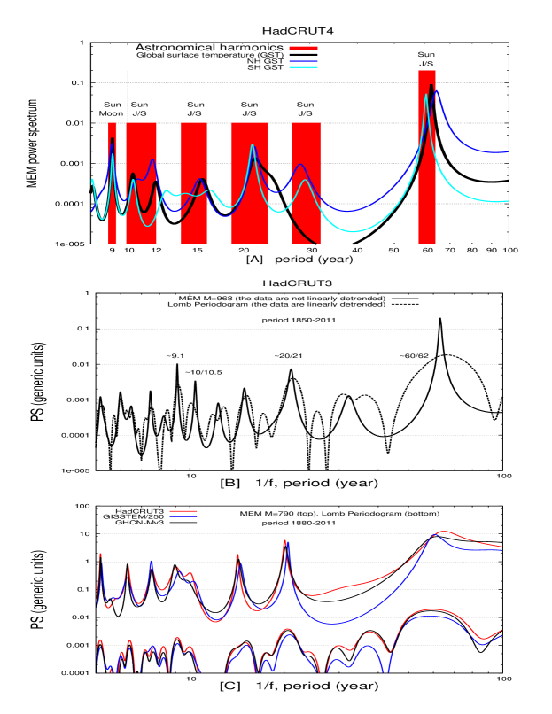
Figure 1: [A] Power spectra of the HadCRUT4 GST (1850-2012) (black) and of the Northern Hemisphere and Southern Hemisphere using the Maximum entropy Method (MEM); red boxes represents major astronomical oscillations associated to a decadal soli-lunar tidal cycle (about 9.1 years), and to the major heliospheric harmonics associated to Jupiter and Saturn gravitational and electromagnetic effects and to solar cycles (about 10-12, 15, 19-22, 59-63 years) [B] MEM and periodogram for HadCRUT3 (1850-2011). [C] MEM and periodogram for HadCRUT3, GISS and NCDC GSTs from 1880 to 2011. See Scafetta (2010, 2012a, 2012b, 2012c, 2012d, 2013a) for details.

Theoretical climate models should ideally be able to predict the observed GST oscillations. In case of significant mismatches, solutions requiring minor adjustments of the models (for example, tweaking the forcings) may be proposed. However, some of the basic physical assumptions of the models may also be flawed. In the latter case new mechanisms need to be identified in order to upgrade the models. Because of non-reducible uncertainties (Curry and Webster, 2011), alternative semi-empirical modeling strategies should also be developed and considered parallel to the analytic GCM methodology.

Scafetta (2012b) tested all Coupled Model Intercomparison Project 3 (CMIP3) GCMs used by the IPCC (2007) and found that those models poorly reconstruct the observed decadal and multidecadal GST oscillations at about 9.1, 10-11, 20 and 60 year periods since 1850. Herein the ability of the GCMs of the Coupled Model Intercomparison Project 5 (CMIP5) to reproduce the historical global surface temperature patterns since 1850 is tested as well. As an alternate, I conjecture that a significant component of the observed GST variations can be more efficiently modeled using a set of astronomically induced harmonics of solar and lunar origin whose mechanisms are not included in the GCMs yet.

A GCM failure to reproduce large natural multidecadal oscillations (periods, amplitudes and phases) has relevant theoretical implications. For example, Figure 9.5a and b published by the U. N. Intergovernmental Panel on Climate Change (IPCC, 2007) (http://www.ipcc.ch/publications_and_data/ar4/wg1/en/figure-9-5.html) show GCM simulations obtained with all adopted natural and anthropogenic forcings (figure 9.5a) and with natural (solar and volcano) forcings alone (figure 9.5b), respectively. The results depicted by this figure were used to claim that more than 90% of the warming observed since 1900 (about $0.8$ ${}^{o}C$) and practically 100% of the warming observed since 1970 (about $0.5$ ${}^{o}C$) could only be explained by anthropogenic forcing (see figure in 9.5a). The reasoning was that when only solar and volcano forcings alone were used the GCMs predicted a slight cooling since 1970 (see figure 9.5b). The theory emerging from these computer simulations is commonly known as the anthropogenic global warming theory (AGWT). However, if the warming observed since 1970 could be produced by a non-modeled multidecadal natural oscillation linked to major ocean and/or astronomical-solar oscillations, then the AGWT should be questioned and/or significantly revised.

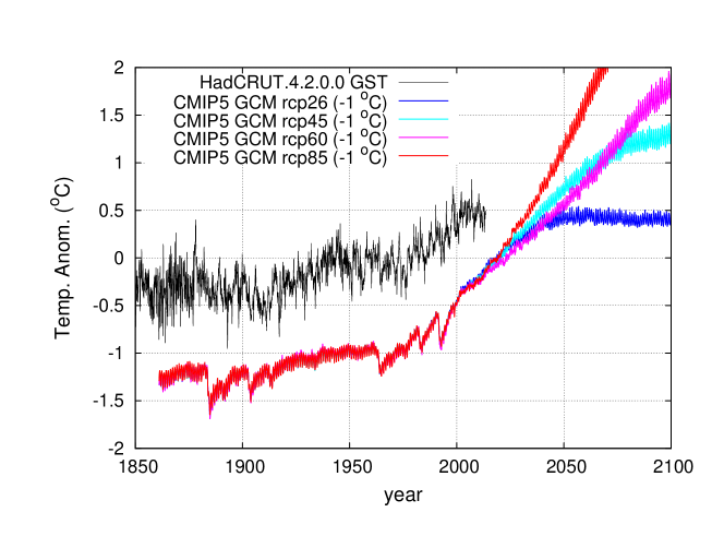
Figure 2: HadCRUT4 global surface temperature record (Jan/1850 - Jun/2013) (black). Four CMIP5 GCM ensemble means based on the historical forcings and four alternative 21st century projections.

The AGWT may be erroneous because of large uncertainties in the forcings (in particular in the aerosol forcing, http://www.ipcc.ch/publications_and_data/ar4/wg1/en/figure-spm-2.html) and in the equilibrium climate sensitivity to radiative forcing. The GCMs used by the IPCC (2007) claim that a doubling of $CO_{2}$ atmospheric concentration induces a warming between 2 and 4.5 ${}^{o}C$ with a total range spanning between 1 and 9 ${}^{o}C$ (see Forest et al. (2006) and http://www.ipcc.ch/publications_and_data/ar4/wg1/en/box-10-2-figure-1.html). The equilibrium climate sensitivity derives from the direct $CO_{2}$ greenhouse warming effect plus the warming contribution its climatic feedbacks. For example, the direct $CO_{2}$ warming would be significantly enhanced by a water vapor feedback since water vapor is a greenhouse gas (GHG) as well. However, the strength and the nature of the various feedbacks is still quite uncertain while the $CO_{2}$ greenhouse properties are experimentally determined and are undisputed: without feedbacks a doubling of $CO_{2}$ amounts to a forcing of about 3.7 $W/m^{2}$ that should cause a warming of about $1~{}^{o}C$ (Rahmstorf, 2008). The strength of the feedbacks is estimated in various ways and also calculated using the GCMs themselves. In the latter case, the calculated climate sensitivity value is a simple byproduct of the physical mechanisms and of the parameters currently implemented in the GCMs such as those related to the parametrization of the cloud formation and water vapor feedbacks (Hansen et al., 1988). If the modeled feedback mechanisms are erroneous, then the modeled climate sensitivity would be inaccurate.

Indeed, some authors have pointed out that observational data indicate that positive and negative climate feedbacks to $CO_{2}$ variations compensate each other, leaving a net equilibrium climate sensitivity to $CO_{2}$ doubling ranging between 0.5 ${}^{o}C$ and 1.3 ${}^{o}C$ (Lindzen and Choi, 2009, 2011; Spencer and Braswell, 2010, 2011). Chylek and Lohmann (2008) found a climate sensitivity between 1.3 ${}^{o}C$ and 2.3 ${}^{o}C$ due to doubling of atmospheric concentration of $CO_{2}$, Ring et al. (2012) found a climate sensitivity between 1.5 ${}^{o}C$ to 2.0 ${}^{o}C$ and Lewis (2013) found a range from 1.2 ${}^{o}C$ to 2.2 ${}^{o}C$ (median 1.6 ${}^{o}C$). The model proposed by Scafetta (2010, 2012b, 2013a), which herein will be reviewed and updated, implies a climate sensitivity from about 0.9 ${}^{o}C$ to 2.0 ${}^{o}C$ (median 1.35 ${}^{o}C$). Moreover, despite some controversy about the tropospheric records (Thorne et al., 2007), NOAA balloon measurements do not show the GCM-predicted $CO_{2}$ induced hot-spot maximum trend in the tropical region at an altitude of about 10 km (Douglass et al., 2007; Singer, 2011). Vonder Haar et al. (2012) showed data that could severely question the existence of a strong GCM global water vapor feedback to anthropogenic GHGs. These findings suggest that current GCMs severely overestimate the climatic effect of the anthropogenic GHG forcing.

As an alternative, I propose a semi-empirical model composed of six major specific astronomically-deduced oscillations spanning from the decadal to the millennial scales (Scafetta, 2010, 2012c). Climatic oscillations can be to a first approximation empirically modeled in particular if they have an astronomical physical origin even if their specific microscopic physical mechanisms remain unknown. Astronomically based harmonic constituent models have been used to predict ocean tides since ancient times (Ptolemy, 2nd century; Kepler, 1601; Ehret, 2008). The oscillations that will be used are found among solar, lunar and planetary harmonics. Climatic effects due to volcano activity and anthropogenic emissions, and the chaotic internal variability of the climate are modeled to a first approximation by properly attenuating the GCM outputs.

It will be shown that the proposed semi-empirical model reconstructs and hindcasts the 1850-2013 climatic patterns significantly better than any CMIP5 GCM simulation and their ensemble mean, and may provide more reliable projections for the 21st century under the same emission scenarios. The finding would suggest that important astronomical forcings of the climate system and the climatic feedbacks to them are still missing and possibly not yet known. The result reinforces Scafetta (2010) where it was found that power spectra of global temperature records are more coherent to solar/astronomical gravitational and electromagnetic oscillations and to soli-lunar tidal long-scale oscillations than to power spectra deduced from current GCM simulations. Therefore, the author proposes that future research should incorporate additional astronomical mechanism of climate change.

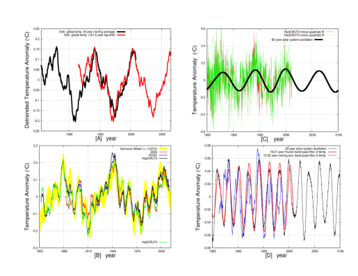
Figure 3: [A] 8-year moving average of the detrended HadCRUT4 GST plotted against itself with a 61.5-year lag shift (red). The quadratic fitting trend applied is $f(t)=0.0000298*(t-1850)^{2}-0.384$. [B] Four GST records (HadCRUT3, HadCRUT4, GISS and NCDC) after being detrended of their upward trend, and smoothed with a 49-month moving average algorithm against the 4-frequency harmonic model (yellow area) proposed in Scafetta (2010, 2012a, 2012c). [C] and [D] show the HadCRUT records detrended of their warming trend and band-pass filtered to highlight their quasi bi-decadal oscillation. The two black oscillating curves with periods of about 20 years and 60 years are two major astronomical oscillations of the solar system induced by Jupiter and Saturn (Scafetta, 2010).

2 Simple analysis of GST and the CMIP5 ensemble mean simulations

All CMIP5 GCM simulations studied were downloaded from Climate Explorer (http://climexp.knmi.nl, for details see also http://cmip-pcmdi.llnl.gov/cmip5). These records are 162 monthly resolved temperature-at-surface (tas) historical simulations from 48 models plus numerous simulations for the 21st century. These are classified under four alternative representative concentration pathway (RCP) emission scenarios labeled as: RCP 8.5 (rcp85), business-as-usual emission scenario; RCP 6.0 (rcp60), lower emission scenario; RCP 4.5 (rcp45), stabilization emission scenario; RCP 2.6 (rcp26), strong mitigation emission scenario. The RCP number indicates the rising radiative forcing pathway level (in $W/m^{2}$) from 2000 to 2100.

Figure 2 compares the HadCRUT4 GST (http://www.cru.uea.ac.uk/) (Morice et al., 2012) from Jan/1850 to Jun/2013 against the CMIP5 model ensemble mean simulations under the four alternative 21st century emission scenarios. The curves are plotted using a common 1900-2000 baseline, with the GCM curves downshifted by 1 ${}^{o}C$ for visual clarity.

The GST warmed about 0.80-0.85 ${}^{o}C$ since 1850. The GST also presents complex dynamical patterns dominated by a quasi 60-year oscillation revolving around an upward trend: 1850-1880, 1910-1940 and 1970-2000 were warming periods, and 1880-1910 and 1940-1970 were cooling periods. Since 2000 the GST has been fairly steady.

period	GST-trend	GCM-trend
1860-1880	+1.01$\pm$0.24	+0.50$\pm$0.06
1880-1910	-0.56$\pm$0.09	+0.28$\pm$0.07
1910-1940	+1.33$\pm$0.08	+0.72$\pm$0.03
1940-1960	-0.47$\pm$0.16	+0.18$\pm$0.04
1940-1970	-0.26$\pm$0.09	-0.33$\pm$0.04
1970-2000	+1.68$\pm$0.08	+1.50$\pm$0.05
2000-2013.5	+0.35$\pm$0.22	+1.88$\pm$0.04

Table 1: Comparison of 30-year period trends in ${}^{o}C/century$ between the HadCRUT4 GST and the CMIP5 GCM ensemble mean simulation depicted in Figure 1.

Figure 3 highlights the GST decadal and multidecadal patterns. Figure 3A shows the HadCRUT4 GST smoothed and detrended of its quadratic polynomial fit and plotted against itself with a lag-shift of 61.5 years. The figure demonstrates that the GST modulation from 1880 to 1940 is very similar to the modulation from 1940 to 2000. This autocorrelation pattern highlights the existence of a possible quasi 60-year oscillation. Additional modulations induced by other patterns may exist. For example, the climate system may also be modulated by a 80-90 year oscillation that has been detected in long solar and climatic proxy records (Knudsen et al., 2011; Ogurtsov et al., 2002; Scafetta and Willson, 2013a). However, a 80-90 year oscillation cannot be separated from a 60-year oscillation using the current GST records, since a 163-year long record is too short.

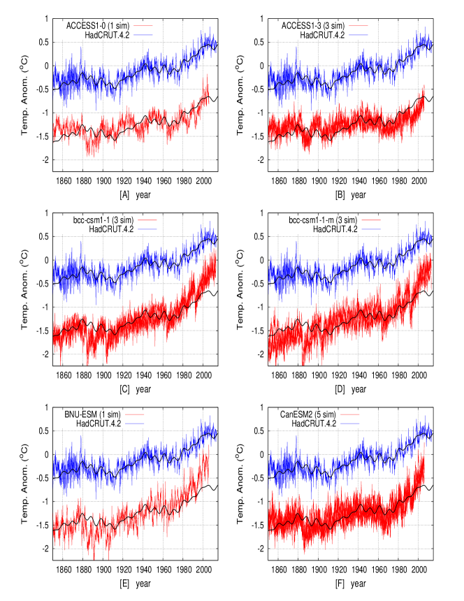
Figure 4: HadCRUT4 GST (blue) vs. CMIP5 GCM simulations (red). Eq. 6 (black). The number of individual available simulations simultaneously plotted is in parenthesis.

Figure 3B highlights both the decadal and the multidecadal GST oscillations by showing four global surface temperature records (HadCRUT3, HadCRUT4, GISS and NCDC) after detrending the upward quadratic trend and smoothing the data with a 49-month moving average algorithm. The harmonic model (yellow) proposed in Scafetta (2010, 2012a, 2012b) approximately reproduces the decadal and multidecadal patterns observed in the detrended GST curves.

Figure 3C shows the HadCRUT3 and HadCRUT4 records detrended of their warming trend as above. Figure 3D shows two band-pass filtered curves of HadCRUT3 (similar pattern is observed for the HadCRUT4 record) to highlight its quasi bi-decadal oscillations. The two black oscillating curves with periods of about 20 years and 60 years are two major astronomical oscillations of the solar system. These can be easily observed, for example, in the speed of the Sun relative to the barycenter of the solar system and in the beats of the gravitational tides induced by Jupiter and Saturn (Scafetta, 2010, 2012a, 2012c, 2013a; Scafetta and Willson, 2013a). The observed climatic oscillations appear synchronized with the two depicted astronomical oscillations. Similar results are obtained with the alternative GST records.

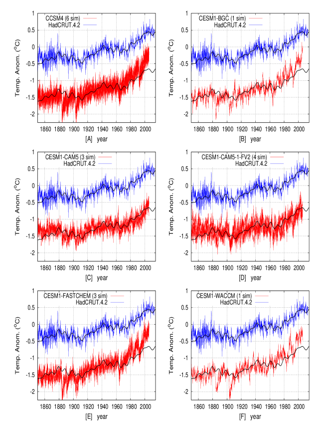
Figure 5: Continues: HadCRUT4 GST (blue) vs. CMIP5 GCM simulations (red). Eq. 6 (black).

Table 1 compares the warming or cooling trends of the HadCRUT4 GST and of the GCM ensemble mean simulations depicted in Figure 2 for the periods 1860-1880, 1880-1910, 1910-1940, 1940-1960, 1940-1970, 1970-2000 and 2000-2013.5: (1) from 1880 to 1910 the GST cooled while the GCMs predict a warming; (2) the 1910-1940 GST warming trend is almost twice than that predicted by the GCMs; (3) the GST cooled since the 1940s while the GCMs predict a warming from 1940 to 1960 which is interrupted by volcano eruptions in the early 1960s; (4) from 1970 to 2000 there is an approximate agreement between the GST and the GCMs; (5) since 2000 a strong divergence between the modeled and observed temperatures is observed. Thus, only during the period 1970-2000 do the GCM simulations present a mean warming trend somewhat compatible with that found in the GST. During the other intervals the GST trends differ significantly from those predicted by the GCM ensemble mean simulations. In particular, the 1910-1940 strong warming and the steady temperature since 2000 cannot be explained by anthropogenic emissions plus a small solar forcing effect, as assumed by the current CMIP3 and CMIP5 GCMs.

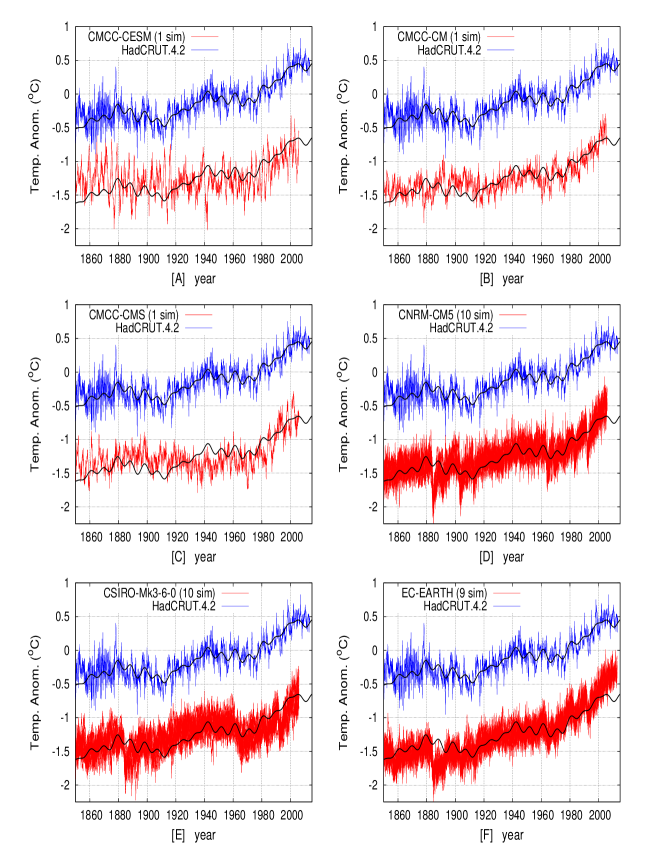
Figure 6: Continues: HadCRUT4 GST (blue) vs. CMIP5 GCM simulations (red). Eq. 6 (black).

Also the GST volcano cooling spikes are not as deep as those predicted by the synthetic record. For example, there is no observational evidence of the strong modeled volcano cooling associated with the eruption of the Krakatau in 1883. Also other volcano signatures appear to be overestimated by the GCMs and produce a spurious recurrence pattern at about 70-80 years (Scafetta, 2012b).

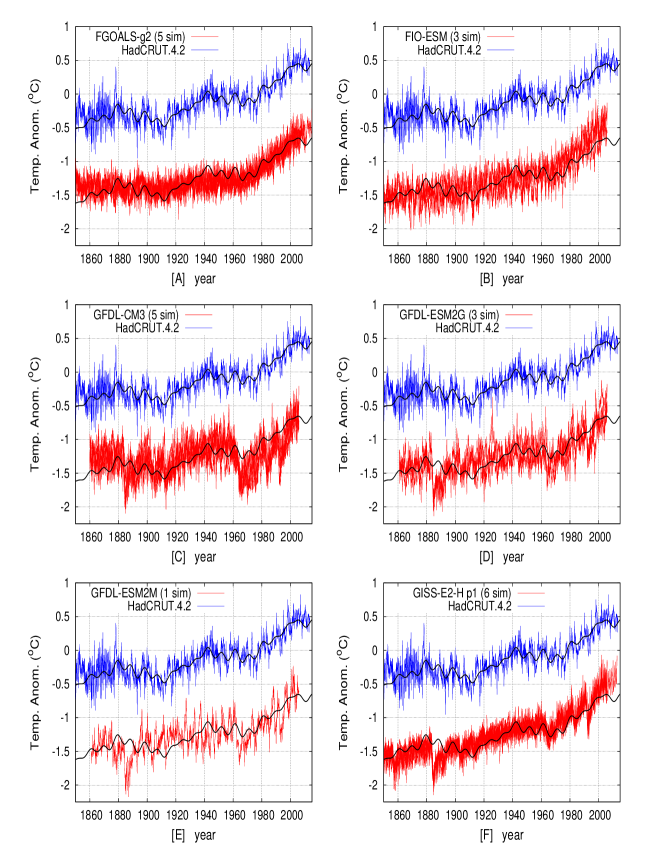
Figure 7: Continues: HadCRUT4 GST (blue) vs. CMIP5 GCM simulations (red). Eq. 6 (black).

These results suggest missing mechanisms and a significant overestimation of the climate sensitivity to the adopted radiative forcings, which is particularly evident in the overestimation of the volcano signatures. On a 163-year period since 1850 only the 1970–2000 warming trend (about 20% of the total period) has been approximately recovered by using known forcings. Thus, the ability of the CMIP5 GCM ensemble mean simulations to project or predict climate change 30 years ahead with any reasonable accuracy is questionable. Indeed, it is possible that the 1970-2000 GCM-data matching could be coincidental and simply due to a fine-tuning calibration of the model parameters to reproduce this period.

3 Scale-by-scale comparison between GST and the CMIP5 simulations

In 48 panels (one for each GCM) Figures 4-11 depict all 162 CMIP5 GCM individual available simulations that are herein analyzed against the HadCRUT4 GST record. The CMIP5 GCM simulations are shifted downward for visual convenience.

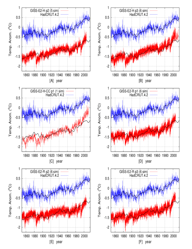
Figure 8: Continues: HadCRUT4 GST (blue) vs. CMIP5 GCM simulations (red). Eq. 6 (black).

The GCM simulations vaguely reproduce a warming from 1860 to 2010. However, significant discrepancies versus the GST record are observed at all time scales. Often the volcano signatures appear significantly overestimated. Some model simulations present a monotonic warming during the entire period, while others show an almost flat temperature trend until 1970 and a rapid rise since then. In a number of cases the 1970-2000 GCM warming rate is visibly higher than the observed 1970-2000 GST warming rate. By looking only at the decadal to the multidecadal scales, numerous mismatches are observed as well. It is easy to notice periods as long as 10-30 years showing divergent trends between the GST record and the GCM simulations. The fast fluctuations at a multi-annual scale are also not reproduced by the models. Indeed, the GCMs reproduce a variability at all time scales, but it appears to be uncorrelated with the GST observations. In general, all GCM simulations significantly differ from each other.

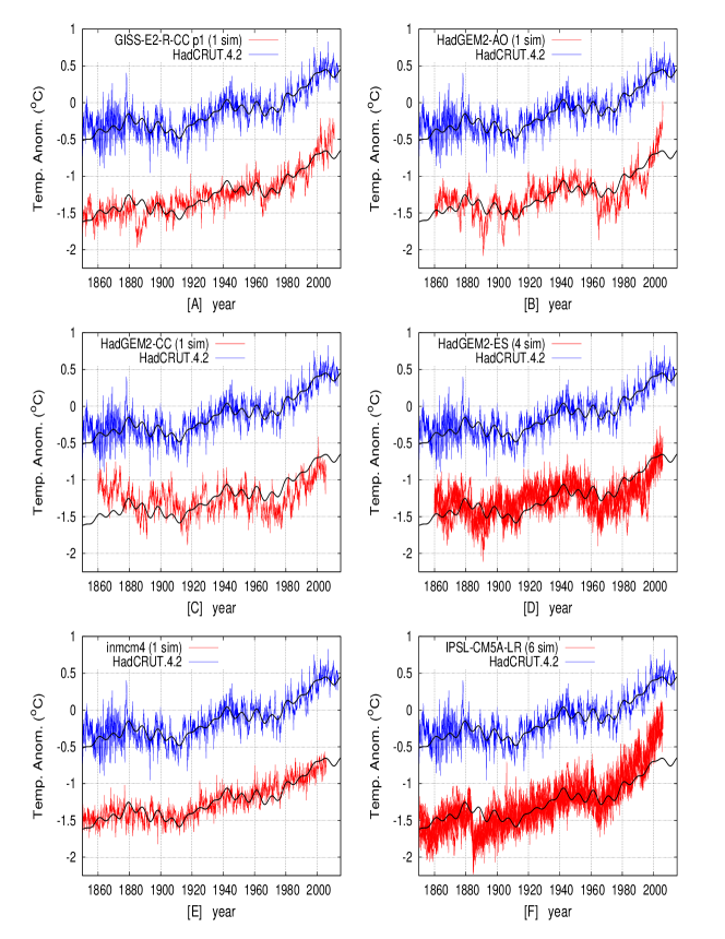
Figure 9: Continues: HadCRUT4 GST (blue) vs. CMIP5 GCM simulations (red). Eq. 6 (black).

In the following subsections three alternative strategies are adopted to study how well the CMIP5 GCM individual simulations reproduce the GST patterns at multiple scales. The following tests are discussed: (1) the records are decomposed using a limited set of major harmonics detected by power spectrum analyses, as shown in Figure 1 and the ability of each GCM simulation to reproduce each GST component is tested; (2) a Fourier band-pass filter decomposition methodology is adopted to decompose each sequence in four band-pass frequency components and the ability of each GCM simulation to reproduce each GST band-pass frequency component is tested; (3) power spectra in the period range from 7 years to 100 years are evaluated for all records and the ability of each GCM simulations to reproduce the GST power spectrum is tested. The scale-by-scale comparison uses a technique similar to the multiresolution correlation analysis (Scafetta et al., 2004). The HadCRUT4 record and all model simulations are analyzed from Jan/1861 to Dec/2005, which is the common period.

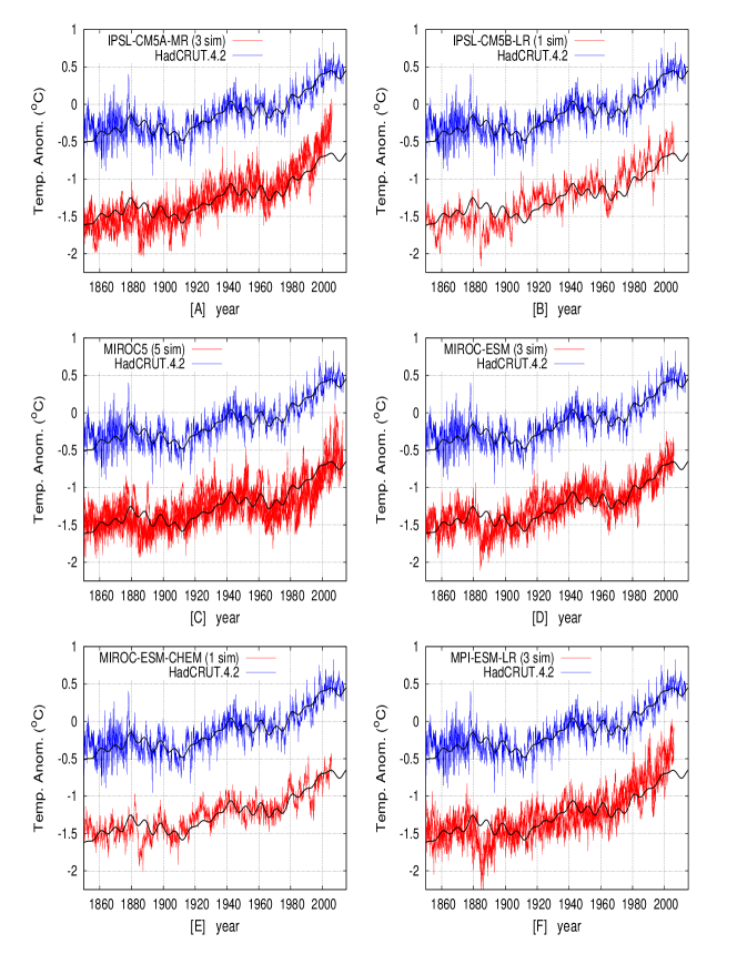
Figure 10: Continues: HadCRUT4 GST (blue) vs. CMIP5 GCM simulations (red). Eq. 6 (black).

3.1 Scale-by-scale harmonic decomposition comparison

Scafetta (2010, 2012a, 2012b) showed that to a first order approximation the HadCRUT3 GST record can be geometrically decomposed into four major harmonics found in astronomical records with periods of about 9.1, 10.4, 20 and 60 years plus a second order polynomial trending component. Here the calibration is repeated using the same harmonics and the HadCRUT4 GST record from Jan/1861 to Dec/2005 to obtain:

$$h_{60}(t) = 0.111\cos(2\pi(t-2001.29)/60)$$ (1)

$$h_{20}(t) = 0.043\cos(2\pi(t-2001.43)/20)$$ (2)

$$h_{10.4}(t) = 0.030\cos(2\pi(t-2002.93)/10.4)$$ (3)

$$h_{9.1}(t) = 0.044\cos(2\pi(t-1997.82)/9.1)$$ (4)

$$p(t) = \frac{3.39}{10^{5}}(t-1850)^{2}-\frac{9.46}{10^{4}}(t-1850)-0.36~{}.$$ (5)

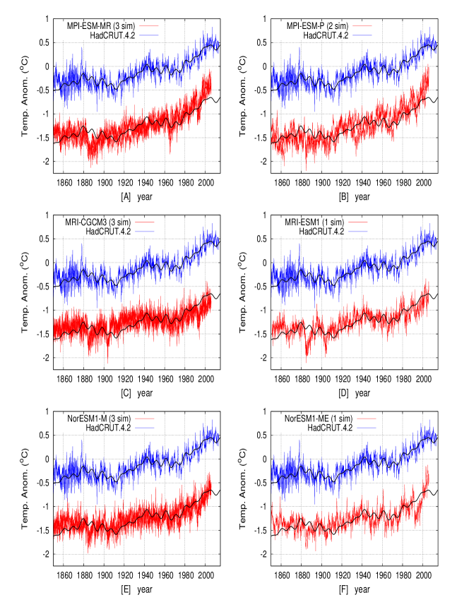
Figure 11: Continues: HadCRUT4 GST (blue) vs. CMIP5 GCM simulations (red). Eq. 6 (black).

The above amplitudes present a statistical error of about 15% and, together with the phases, they were estimated by linear regression on the GST. This yields the following function:

$$f(t)=h_{60}(t)+h_{20}(t)+h_{10.4}(t)+h_{9.1}(t)+p(t).$$ (6)

Eq. 6 is plotted in black in Figures 4-11 and reproduces the decadal and multidecadal GST patterns relatively well. Figures 4-11 also plot Eq. 6 against the GCM simulations on the common baseline. The latter comparison assists a visual check of the ability of the GCM simulations to reproduce the decadal and multidecadal GST patterns, which is generally poor.

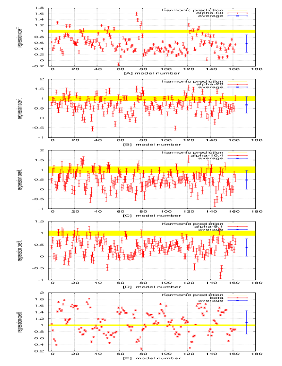
Figure 12: Regression coefficients calculated using Eq. 7 referring to all GCM runs, as reported in Table 2. The GCM number -0- corresponds to the CMIP5 model mean simulation depicted in Figure 2. The yellow area around 1 corresponds to the harmonic model confidence region. The blue bars are the average values with relative error bars.

Note that $p(t)$ is only a convenient second order polynomial geometrical description of the upward warming trend from Jan/1861 to Dec/2005. This function does not have any hindcasting or forecasting ability outside the interval 1861–2005 because its derivation is geometrical, not physical. The justification of $p(t)$ is purely mathematical and derives directly from Taylor’s theorem. Essentially, a second order polynomial is used because this function is required to capture the accelerating GST warming trend from 1861 to 2005. Simultaneously, it should be as orthogonal as possible to a 60-year cycle on a 145-year period: see also Scafetta (2013b, figure 4). In section 5 the geometrical function $p(t)$ is substituted with a more physically-based function by taking into account secular and millennial cycles (Humlum et al., 2011; Scafetta, 2012c, 2013a) plus the contribution from volcano and anthropogenic forcings.

In contrast, the four chosen harmonics are supposed to represent real dynamical mechanisms related to astronomical cycles. Thus, they may have, within certain limits, hindcast/forecast capabilities outside the interval 1850-2010, as it was explicitly tested in multiple ways (Scafetta, 2010, 2012a, 2012b, 2012c). However, numerous other harmonics may exist, as it happens for the tidal system where up to 40 harmonics are used. Additional harmonics are ignored in this analysis.

The GCM simulations should simultaneously reproduce harmonics and an upward trend statistically compatible with those found in the GST record. Thus, we use the same strategy implemented in Scafetta (2012b), and adopt the following regression model

$$\begin{split}g(t)=\alpha_{60}h_{60}(t)+\alpha_{20}h_{20}(t)+\alpha_{10.4}h_{10.4}(t)\\ +\alpha_{9.1}h_{9.1}(t)+\beta p(t)+\gamma\end{split}$$ (7)

where $\alpha$, $\beta$ and $\gamma$ are appropriate regression coefficients that are evaluated for each GCM simulation, $m(t)$, by using the usual minimization of the residual square function, $\sum_{x}[m(t)-g(t)]^{2}$, during the period Jan/1861 - Dec/2005. The parameter $\gamma$ has only a baseline meaning.

If the evaluated regression coefficients $\alpha$ and $\beta$ are close to 1, then the GCM simulation could well reproduce the corresponding temperature constituent pattern captured by Eq. 6. For example, if $\alpha_{60}\approx 1$, then the analyzed GCM simulation function, $m(t)$, could reconstruct the 60-year modulation found in the temperature record as captured by the constituent function $h_{60}(t)$. However, such a condition is necessary but not sufficient to guarantee the matching between the two records at the given frequency. On the contrary, if the evaluated regression coefficients are statistically different from 1, then the GCM simulation can not reconstruct the correspondent GST pattern.

Table 2 reports the six regression coefficients $\alpha$, $\beta$ and $\gamma$ for the ensemble mean and for each of the 162 GCM simulations. These results are also depicted in Figure 12. The results are quite unsatisfactory. All GCM simulations fail to reproduce the four decadal and multidecadal GST oscillations sufficiently well.

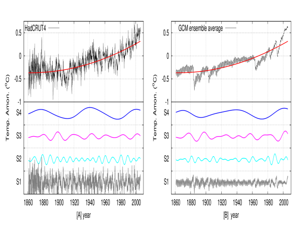
Figure 13: Scale-by-scale Fourier band-pass frequency decomposition: [A] HadCRUT4 GST; [B] GCM ensemble mean. Quadratic polynomial fit, Eq. 5 (red). S1 captures time-scales shorter than 7 years; S2 captures scales between 7 and 14 years; S3 captures scales between 14 and 28 years; S4 captures scales between 28 and 104 years. Note in [A] the clear quasi 60-year oscillation in the HadCRUT4 GST S4 record and the beat modulation in the HadCRUT4 GST S2 curve caused by the 9.1 and 10.4 year oscillations.

The averages of the 162 results give values between 0.4 and 0.7 with a standard deviation between 0.3 and 0.5. Thus, most regression coefficients fall outside the yellow area of the harmonic model confidence reported in the first line of Table 2. Even if occasionally a regression coefficient falls close to 1, as shown in Figure 13, it is likely a coincidence as the GCM simulations should simultaneously reproduce all decadal and multidecadal patterns. A comprehensive statistical test is provided by using the following reduced $\chi^{2}$ values that are reported in Table 2 and are defined as:

$$\begin{split}\chi^{2}=&\frac{1}{5}\left[\frac{(\alpha_{60m}-\alpha_{60T})^{2}}{\Delta\alpha_{60m}^{2}+\Delta\alpha_{60T}^{2}}+\frac{(\alpha_{20m}-\alpha_{20T})^{2}}{\Delta\alpha_{20m}^{2}+\Delta\alpha_{20T}^{2}}+\right.\\ &\frac{(\alpha_{10.4m}-\alpha_{10.4T})^{2}}{\Delta\alpha_{10.4m}^{2}+\Delta\alpha_{10.4T}^{2}}+\frac{(\alpha_{9.1m}-\alpha_{9.1T})^{2}}{\Delta\alpha_{9.1m}^{2}+\Delta\alpha_{9.1T}^{2}}+\\ &\left.\frac{(\beta_{m}-\beta_{T})^{2}}{\Delta\beta_{m}^{2}+\Delta\beta_{T}^{2}}\right].\end{split}$$ (8)

The suffix ‘m’ indicates the correspondent regression coefficient for the GCM model; the suffix ‘T’ indicates the correspondent regression coefficient for the harmonic model reported in the first line of Table 2. Values of $\chi^{2}\lessapprox 1$ would indicate that the model performs well in reproducing the decadal and multidecadal patterns shown in the data. However, as the table reports, $\chi^{2}$ varies between 3.5 and 161 (mean=$51$) among the 162 individual simulations. $\chi^{2}$ is 14 for the ensemble mean model. Values $\chi^{2}\gg 1$ indicate that these GCMs do not reconstruct the GST decadal and multidecadal scales.

Table 2 also reports the root mean square deviation
(RMSD) from Eq. 6 for both the GST record and for all GCM simulations shown in Figure 4-11: $RMSD(\xi,\theta)=$
$\sqrt{\sum_{i=1}^{N}(\xi_{i}-\theta_{i})^{2}/N}$. This function measures the ability of a simulated sequence, $\{\xi_{i}\}$, to reconstruct the observed sequence, $\{\theta_{i}\}$. The RMSD is calculated after both the GST record and the GCM simulations are smoothed with a 49-month moving average algorithm to highlight the decadal modulation, as done in Figure 3B. For the GCMs, RMSD ranges between 0.08 ${}^{o}C$ and 0.22 ${}^{o}C$, with an average of 0.14 ${}^{o}C$. On the contrary, the harmonic model (Eq. 6) presents a RMSD of 0.05 ${}^{o}C$, indicating that the latter is statistically more accurate in representing the GST records by a factor between 2 and 4.4 compared with the CMIP5 GCMs, as also found for the CMIP3 GCMs (Scafetta, 2012b).

3.2 Scale-by-scale band-pass filter decomposition comparison

A Fourier band-pass filter decomposition captures all dynamical details of a time sequence at complementary time-scales. Figures 13A and 13B show the decomposition of the HadCRUT4 GST and of the GCM ensemble mean simulation. S1 corresponds to time-scales larger than 6 months and shorter than 7 years, and captures most of the fast variability of the signal such as ENSO oscillations and volcano eruptions; S2 corresponds to scales between 7 and 14 years, and captures the decadal scale; S3 corresponds to scales between 14 and 28 years, and captures the bi-decadal oscillation; S4 corresponds to scales between 28 and 104 years, and captures the multidecadal scale such as the quasi 60-year oscillation. A second order polynomial, given by Eq. 5, is detrended from all sequences to make them stationary to a first order approximation.

If $T_{c}(t)$ is a measured band-pass temperature component function, and $M_{c}(t)$ is the correspondent GCM temperature band-pass component function, the regression coefficient $\Phi$ is given by the formula

$$\Phi=\frac{\sum M_{c}(t)T_{c}(t)}{\sum T_{c}(t)T_{c}(t)}~{}.$$ (9)

If $\Phi$ is close to 1, then the functions $M_{c}(t)$ and $T_{c}(t)$ are statistically compatible according to this measure. Again, such a condition is necessary but not sufficient to guarantee the matching between the two records at the given frequency band.

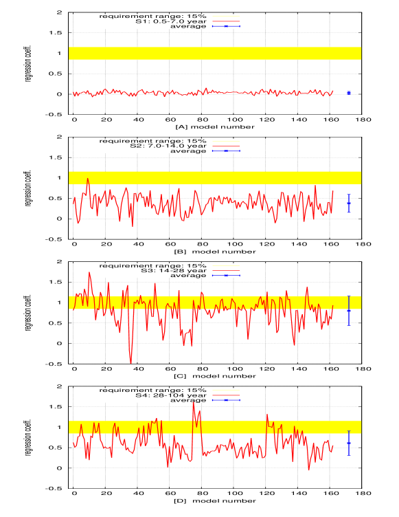
Figure 14: Regression coefficients $\phi$ calculated using Eq. 9 referring to all GCM runs, as reported in Table 3: [A] $\phi_{S1}$, band-pass range 0.5-7.0 year; [B] $\phi_{S2}$, band-pass range 7.0-14.0 year; [C] $\phi_{S3}$, band-pass range 14-28 year; [D] $\phi_{S4}$, band-pass range 28-104 year. The GCM number -0- corresponds to the CMIP5 model mean simulation depicted in Figure 1. The yellow area around 1 corresponds to the chosen confidence region of 15%. The blue bars are the average values with relative error bars.

Table 3 reports the four scale-by-scale regression coefficients calculated for the GCM ensemble mean and the 162 GCM simulations versus the correspondent GST frequency band-pass components. The same coefficients are depicted in Figure 14. All GCM simulations, including the GCM ensemble mean (number -0- in the figure), perform much less well in reconstructing the temperature components although occasionally a single regression coefficient may fall close to 1. The average values relative to the four band-pass components are statistically different from $\langle\Phi\rangle=1\pm 0.15$ (a reasonable 15% error from the ideal $\Phi=1$ is assumed for all values as approximately found in Table 2 for the harmonic model components): for S1, $\langle\Phi\rangle=0.03\pm 0.04$; for S2, $\langle\Phi\rangle=0.38\pm 0.22$; for S3, $\langle\Phi\rangle=0.80\pm 0.36$; for S4, $\langle\Phi\rangle=0.61\pm 0.30$.

Table 3 also reports a reduced $\chi^{2}$ test using an equation similar to Eq. 13. However only the three components related to the S2-scale, S3-scale and S4-scale are used in the test as

$$\chi^{2}=\frac{1}{3}\left[\frac{(\Phi_{S4}-1)^{2}}{0.15^{2}}+\frac{(\Phi_{S3}-1)^{2}}{0.15^{2}}+\frac{(\Phi_{S2}-1)^{2}}{0.15^{2}}\right].$$ (10)

The S1-scale is excluded because the GCM models evidently do not reconstruct the fast fluctuations at scales shorter than 7 years. Again, $\chi^{2}\gg 1$ for all models. Thus, as in the previous subsection, also these results suggest that the CMIP5 GCMs do not properly reconstruct the observed GST dynamics at multiple time scales, although a significant variation among the individual simulations is observed.

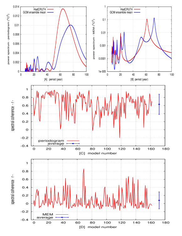
Figure 15: [A] Periodograms of the GST record (red) and of the GCM ensemble mean simulation (blue); [B] Maximum entropy method (MEM) power spectrum of the GST record (red) and of the GCM ensemble mean simulation (blue); [C] Spectral correlation coefficients between the GST recorcd and all GCM simulations using the periodograms; [D] Spectral correlation coefficients between the GST record and all GCM simulations using the MEM power spectra. See Table 3, last two columns.

3.3 Direct power spectrum comparison

Figure 15 depicts a final statistical test that estimates the ability of the GCMs in reconstructing the power spectrum of the GST within the period range from 7 to 100 years.

Figure 15A shows in red the periodogram of the HadCRUT4 GST and of the GCM ensemble mean; Figure 15B shows in red the maximum entropy method (MEM) power spectrum of the HadCRUT4 GST and of the GCM ensemble mean. The periodogram and MEM algorithms were taken from Press et al. (1997) and calculated after detrending from all records Eq. 5. The figures highlight, for example, that the GCM ensemble mean macroscopically fails to reproduce the quasi 60-year oscillation by presenting a spectral peak at a period of $\sim 75$ years instead of the observed $\sim 61$ years: see also Figure 3A.

As alternatively demonstrated in Scafetta (2012b, figure 2) the autocorrelation peak at a time-lag of 70-80 years found in the GCM simulations is mostly driven by the strong GCM volcano eruption signatures. In fact, there is a quasi 80-year lag between the two GCM large volcano eruption signatures of Krakatoa (1883) and Agung (1963-1964), and between the volcano signatures of Santa Maria (1902) and El Chichon (1982). Note that the quasi 80-year recurrent pattern in the volcano signature could have been responsible for the slight shift of the peak of the GST periodogram at a value slightly larger than 60 years, as mostly observed in Figure 15A.

A coherence test is made by simply calculating the cross-correlation coefficient $r$ between the GST power spectrum depicted in the figure and each of the GCM power spectra. Values of $r$ close to 1 indicate a good spectral coherence between the GST record and the GCM simulations. Note, however, that this is a less stringent test than the cases discussed in subsections 3.1 and 3.2 because a mere power spectrum correlation test ignores the phase positions of the harmonics which is a necessary component that the models should reconstruct as well.

The comparison between the GST record and the GCM ensamble mean record gives $r=0.79$ using the periodograms, and $r=-0.02$ using the MEM power spectra, which present sharper peaks. The test is repeated for all 162 GCM simulations. The results are depicted in Figues 15C and 15D and reported in the last two columns of Table 3. The average correlation coefficient is $\langle r\rangle=0.63\pm 0.25$ using the periodograms and $\langle r\rangle=0.08\pm 0.21$ using the MEM power spectra.

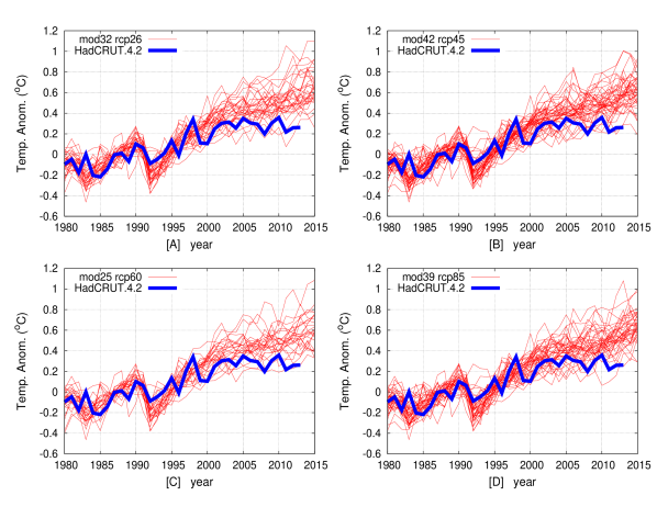
Figure 16: HadCRUT4 record (blue) versus the CMIP5 GCM projections: [A] the rcp26 simulations made of 32 models; [B] the rcp45 simulations made of 42 models; [C] the rcp60 simulations made of 25 models; [D] the rcp85 simulations made of 39 models. All records are annually resolved and baselined in the 1980-2000 period. Note that in 2013 the temperature, which is approximately steady since 1997, runs cooler than all CMIP5 GCM simulations.

Thus, the GCMs do not reproduce the natural harmonics of the climate system even in the less stringent sense of a mere power spectrum correlation test that ignores the phase positions of the harmonics. These results indicate a relatively poor spectral coherence at the dacadal and multidecadal scale between the GST and the GCM simulations. The performance of the individual GCM simulations varies greatly.

4 Visual examples of CMIP5 GCM deficiencies

Typical major deficiencies found in the GCM simulations are briefly discussed in the following two subsections. A simple visual analysis of the records suffices to highlight severe mismatches between the GCM simulations and the GST record.

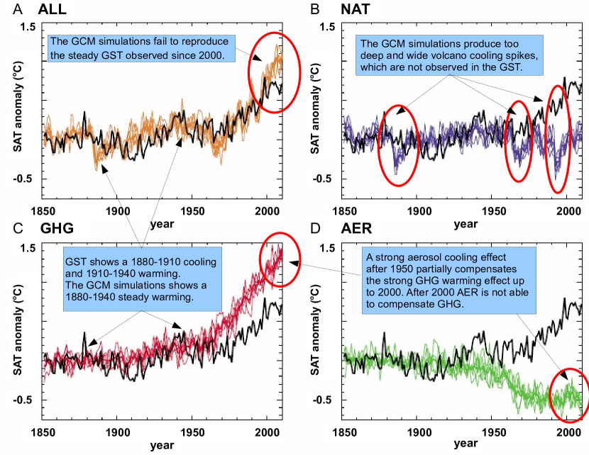
Figure 17: A reproduction of figure 1 in Gillett et al. (2012) with additional comments that highlight major mismatches between the GST record (black) and a set of simulations made with CanESM2. The figure highlights problems common to all CMIP5 GCMs.

4.1 Example 1: the GCM simulations significantly diverge from the GST record since 2000

Most CMIP5 GCM simulations using the historical forcings end in Dec/2005. Since 2006 the models are run using projected forcings for the 21st century. Four scenarios have been proposed and labeled as: rcp26, rcp45, rcp60, rcp85, as also shown in Figure 2.

Figure 16 shows the annually resolved available simulations in the four cases versus the annually resolved HadCRUT4 record (the 2013 value is based on data from January to June). The records are baselined during the period 1980-2000. The rcp26 simulations are made of 32 models, rcp45 of 42 models, rcp60 of 25 models and rcp85 of 39 models.

Figure 16 clearly shows that the models have significantly overestimated the global warming rate since 2000: see also the detailed analysis proposed by Fyfe. For the year 2013 all models have predicted a global mean surface temperature that is found to be 0.0-0.5 ${}^{o}C$ warmer than the GST record. The linear rate of the HARCRUT4 record since 2000 is $0.3\pm 0.4$ ${}^{o}C/century$, which indicates that no warming has been observed in the GST record since 2000. In contrast, the CMIP5 simulations have predicted a strong warming rate of: [A] rcp26, $2.2\pm 0.2$ ${}^{o}C/century$; [B] rcp45, $2.1\pm 0.2$ ${}^{o}C/century$; [C] rcp60, $1.9\pm 0.2$ ${}^{o}C/century$; [D] rcp85, $2.1\pm 0.2$ ${}^{o}C/century$.

4.2 Example 2: a detailed qualitative visual study of the CanESM2 GCM simulations

Figure 17 reinterprets figure 1 of Gillett et al. (2012) that compares the GST record and a set of simulations of CanESM2 GCM, which produces some of the best results among all GCMs. For example its simulations produce the best multidecadal result with a $3<\chi^{2}<15$ (see Tables 2-3 and the correspondent figures). However, even the CanESM2 simulations macroscopically fail to reproduce the observed steady GST pattern since 2000. CanESM2 appears to be finely tweaked with the aerosol uncertain forcing, but still fails to reconstruct important temperature patterns, which are far better reconstructed by the harmonic model discussed in Section 6. In fact, for the CanESM2 simulations RMSD ranges from 0.13 to 0.15 ${}^{o}C$ while Eq. 13 has a RMSD of about 0.04 ${}^{o}C$.

In the simulations depicted in Figure 17, CanESM2 GCM is forced with: (a) anthropogenic and natural forcings (ALL), (b) natural forcings only (NAT), (c) greenhouse gases only (GHG), and (d) aerosols only (AER). The comments added to the figure highlight typical common problems found in all CMIP5 GCMs when compared with the GST record. (1) The GCM does not reproduce the 2000-2012 steady GST trend. (2) The volcano cooling spikes are too large compared to the signature that can be qualitatively deduced from the GST record. (3) GST shows a clear 60-year modulation made of a 1880-1910 cooling plus a 1910-1940 warming, while the GCM shows a 1880-1940 steady warming. (4) The GCM needs a strong aerosol cooling effect after 1950 to partially compensate the strong GHG warming effect up to 2000, but after 2000 the aerosol cooling effect is not able to compensate the strong GHG warming effect, and the simulations strongly diverge from the observations.

5 Discussion

The general failure of the CMIP5 GCMs to accurately reconstruct the dacadal and multidecadal GST scales, including that the GST has not warmed during the last 17 years (essentially since about 1997), brings into question the reliability of these models. In fact, Knight et al. (2009) observed that: “Near-zero and even negative trends are common for intervals of a decade or less in the simulations, due to the model’s internal climate variability. The simulations rule out (at the 95% level) zero trends for intervals of 15 year or more, suggesting that an observed absence of warming of this duration is needed to create a discrepancy with the expected present-day warming rate.” The results of this analysis suggest that major physical flaws exist in the CMIP3 and CMIP5 GCMs, which may cast doubts on their 21st century projections as well.

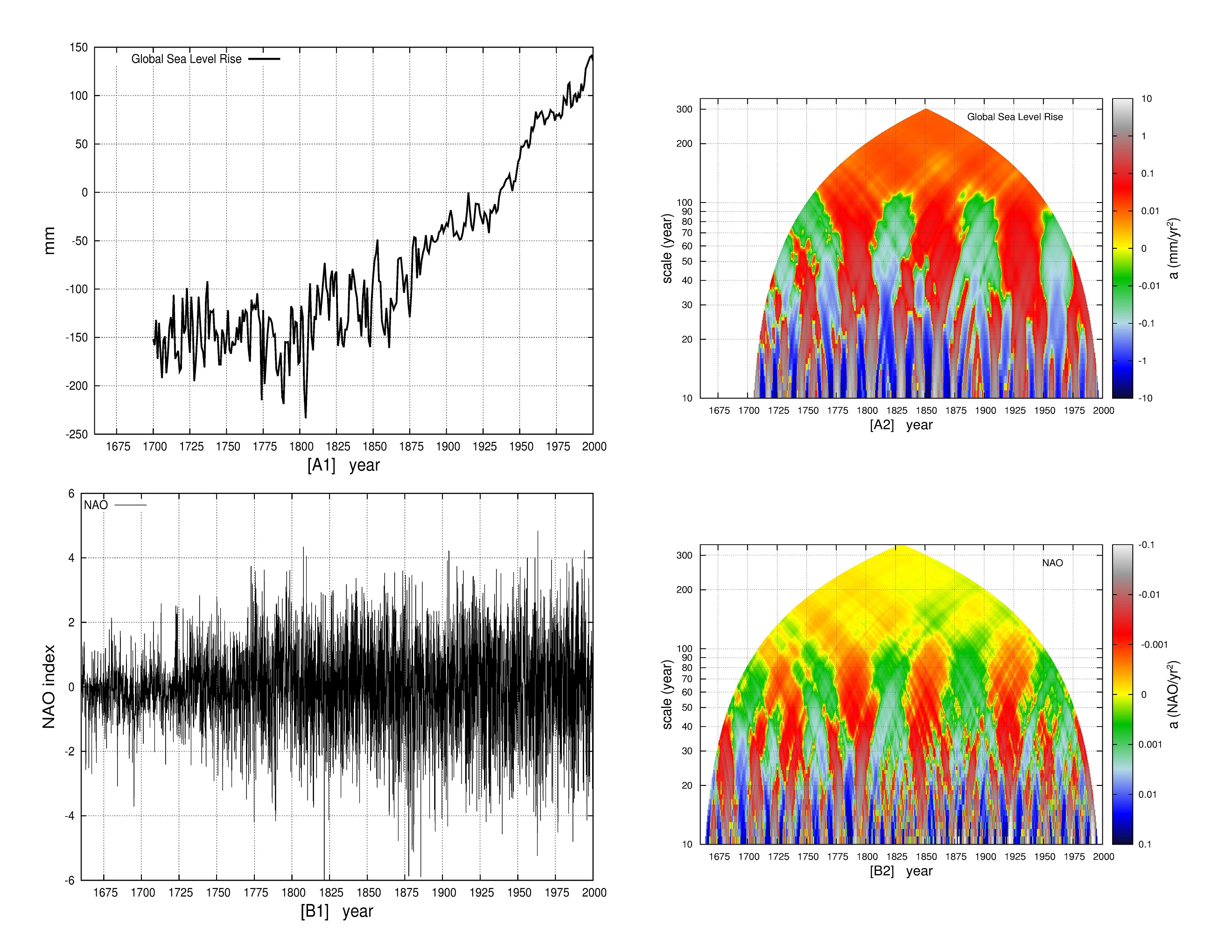
Figure 18: [A] Global sea level record (Jevrejeva et al., 2008) (left) and its MSAA colored diagram (right). [B] North Atlantic Oscillation (NAO) (Luterbacher et al., 1999, 2002) (left) and its MSAA colored diagram (right). In [B] the colors are inverted. Note the common quasi 60 year oscillation since 1700 indicated by the alternating green and red regions within the 30-100 year scales. From Scafetta (2013c).

The inability of the GCMs to model the observed oscillations and, in particular, the post-2000 temperature plateau has been justified in various ways. In general, it has been speculated that the models and/or their forcings need to be slightly corrected. Effects of missing volcano forcing, aerosol forcing and/or some internal unforced dynamics of the climate system have typically been speculated, but problems arise with these interpretations.

For example, Booth et al. (2012) speculated that the cooling from 1940 to 1970 was due to poorly modeled aerosol forcing. However, the temperature also presents an equivalent cooling period from 1880 to 1910 that was not reconstructed by their model. Kaufmann et al. (2011) speculated that the steady GST between 1998-2008 was caused by an increase of atmospheric sulfate production (primarily from China) that countered the greenhouse gas warming. However, Remer et al. (2008) (see their figure 5) showed no change in global aerosol optical depth during the period 2000-2007. Meehl et al. (2011) speculated that GST hiatus periods could be caused by occasional deep-ocean heat uptake, and showed that GCM simulations may occasionally present, at random times, an up-to-a-decade of steady temperature despite an increasing anthropogenic forcing. However, the CCSM4 GCM used in Meehl et al. (2011) (which is one of the models analyzed above) does not reproduce the steady temperature observed from 2000 to 2013. The CCSM4 GCMs only produce hiatus periods occurring in 2040-2050 and 2070-2080, which appear as random red-noise fluctuations of the model (see their figure 1a). The latter variability is commonly referred to as internal unforced dynamics of the climate system and it is claimed to be unpredictable.

However, because the lack of warming since 1997–1998 is just an aspect of the problem, the above speculations appear physically unsatisfactory. A comprehensive and consistent theory of climate change must simultaneously interpret the entire GST dynamics observed since 1850 at least from the decadal scale up. Although aerosols and internal dynamics certainly may have some effects, the GST also appears to present quasi regular oscillations. The findings of the previous sections indicate that the CMIP5 GCMs fail to simultaneously capture the decadal and multidecadal GST dynamical patterns observed since 1850 such as the four identified major oscillations with approximate periods of 9.1, 10-11, 20 and 60 years (Scafetta, 2010). These oscillations generate a network of dynamical synchronization within the climate system also not reproduced by the models (Wyatt et al., 2011). The tables 2 and 3 show that the GCM performance varies greatly both among the models and among the individual model runs produced by the same model.

Quasi-decadal, bidecadal and 60-year oscillations and other longer oscillations have been detected in numerous records covering centuries and millennia. For example, Jevrejeva et al. (2008) and Chambers et al. (2012) showed a quasi 60-year cycle in the sea level rise rate since 1700; Klyashtorin et al. (2009) showed that numerous climate indexes present a long-term 50-70 year oscillations during the last 1500 years; Knudsen et al. (2011) showed a persistent quasi 60-year cycle in the Atlantic Multidecadal Oscillation throughout the last 8,000 years; a quasi 20-year and 60-year oscillations also appear for centuries and millennia in some Greenland temperature records (Davis and Bohling, 2001; Chylek et al., 2012). The Introduction section contains additional suggested references showing these oscillations.

For example, Figure 18 reproduces figure 10 in Scafetta (2013c) that shows two relatively global climatic indexes since 1700: the global sea level record (Jevrejeva et al., 2008) and the North Atlantic Oscillation (NAO) reconstruction (Luterbacher et al., 1999, 2002). The right panels show the multi-scale acceleration analysis (MSAA) of these two records and highlight the presence of a common major quasi 60-year oscillation since 1700. This oscillation is revealed by the alternating green and red colors indicating that the local acceleration of the records varies from negative to positive values, that is, there is an oscillation.

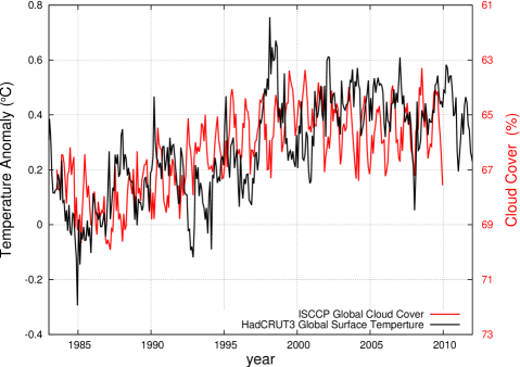
Figure 19: Global surface temperature (black) against monthly variations in total global cloud cover since July 1983 (red). Correlation coefficient: $r_{o}=-0.52$, for 318 points $P(|r|\geq|r_{o}|)<0.0005$. The cloud data are from the International Satellite Cloud Climatology Project (ISCCP). Cloud data from http://isccp.giss.nasa.gov/pub/data/D2BASICS/B8glbp.dat

The existence of large quasi-60 year oscillations lasting centuries (for example, Scafetta et al. (2013) found a quasi-60 year oscillation in the ice core GISP2 temperature record since 1350) questions interpretations such as that proposed by Imbers et al. (2013) that the quasi 60-year modulation observed in the GST record since 1850 could be due to some kind of red noise produced by short memory processes exemplified by AR(1) models or by long memory processes, which were claimed to modulate the internal variability of the global mean surface temperature. In fact, a generic stochastic model would not be able to reproduce a quasi harmonic signal lasting centuries in an energetically dissipative system such as the climate without the help of a specific harmonic forcing.

Indeed, the climate system appears to be chaotically oscillating around a dominant complex harmonic component made of multiple specific frequencies plus some additional contribution from volcano and anthropogenic forcings. The internal variability more likely chaotically perturbs the oscillations, but does not produce them. This harmonic component looks complex but also predictable. It appears more similar in principle to the tidal oscillations of the ocean, which are forced by numerous astronomical harmonics, than to a hypothetical random internal unforced dynamics of the climate system.

Evidence has been presented that the observed decadal and multidecadal oscillations might have an astronomical origin (Scafetta, 2010, 2012a, 2012b, 2012c, 2012d, 2013a).

For example, the quasi 9.1-year oscillation appears to be related to long solar/lunar tidal oscillations: see also Keeling and Whorf (1997a) and Wang et al. (2012). The rationale is the following. The lunar nodes complete a revolution in 18.6 years, and the Saros soli-lunar eclipse cycle completes a revolution in 18 years and 11 days. These two cycles induce 9.3 year and 9.015 year tidal oscillations corresponding respectively to Sun-Earth-Moon and Sun-Moon-Earth tidal configurations. Moreover, the lunar apsidal precession completes one rotation in 8.85 years causing a corresponding lunar tidal cycle. Thus, three interfering major soli-lunar tidal cycles clustered between 8.85 year and 9.3 year periods are expected, which should generate a major varying oscillation with an average period around 9.06 years. This soli-lunar tidal induced cycle could peak, for example, in 1997-1998 when the solar and lunar eclipses occurred close to the equinoxes (this happens every $\sim 9$ years) when the soli/lunar tidal torque is reasonably at the equator. In general, it is evident that the GST can be influenced by oceanic oscillations induced by soli-lunar gravitational tides, which produce a very complex set of harmonics at multiple time scales (Keeling and Whorf, 1997a, b; Wang et al., 2012).

The other decadal and multidecadal oscillations shown in Figure 1 appear to be mostly related to solar/planetary oscillations induced by Jupiter and Saturn and are seen in the solar wobbling and in the solar activity. These astronomical oscillations are indicated by the black curves depicted in Figure 2C and 2D which refer to the speed of the sun relative to the barycenter of the solar system. Scafetta analysed several other multisecular proxy temperature models and also showed that it is possible to hindcast the 1950-2010 GST oscillations using a harmonic model calibrated on the period 1850-1950, and vice versa.

There is considerable empirical evidence showing a strong correlation between climate and solar records at multiple scales (Hoyt and Schatten, 1997; Bond et al., 2001; Kerr, 2001; Kirkby, 2007; Svensmark, 2007; Svensmark and Friis-Christensen, 2007; Steinhilber et al., 2012; Kokfelt and Muscheler, 2013). Numerous authors (e.g.: Scafetta and West, 2007; Scafetta, 2009a; Kirkby, 2007, etc) have argued that to interpret recent paleoclimate temperature reconstructions and their patterns since the Maunder solar minimum (1640-1715), it is necessary to postulate a climatic response to solar variations significantly larger than that predicted by the current GCMs. GCMs assume the existence of a total solar irradiance (TSI) forcing although this is a very small contribution to climate change (IPCC, 2007). However, a 1-3% astronomically-induced modulation of the Earth’s albedo can easily provide the strong needed climatic amplification effect to solar variation up to a factor of 10. For example Scafetta (2012a) calculated that differentiating directly the Stefan–Boltzmann’s black-body equation a climate sensitivity of $k_{S}=0.053~{}K/Wm^{-2}$ is found (this value uses the metric adopted in Scafetta (2012a) which differs from the common metric). However, if a solar activity variation of 1 $W/m^{2}$ induces also a 1% variation of the albedo, a climate sensitivity of $k_{S}=0.36~{}K/Wm^{-2}$ would be found, which is about an order of magnitude larger than the previous value.

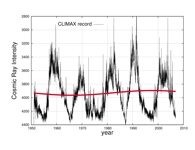
Figure 20: CLIMAX cosmic ray count. The scale is inverted because cosmic ray flux is negatively correlated with solar activity. The figure suggests that solar activity might have increased on average from 1970 to 2000 (similarly to ACRIM TSI satellite composite (Willson and Mordvinov, 2003; Scafetta and Willson, 2009)) causing a global warming by inducing a decrease in the cloud cover (observed in the data, Figure 19) via a reduction of cosmic ray flux. The red curve is a simple regression model made of a linear trend plus a 60-year oscillation used to highlight the multidecadal modulating pattern. Data from http://ulysses.sr.unh.edu/NeutronMonitor/Misc/neutron2.html .

Scafetta and Willson (2013a) found evidence for a quasi 60-year oscillation (and others) in aurora records since 1530 linked to astronomical oscillations. If electromagnetic space weather mechanisms induce small oscillations in the upper strata of the atmosphere that drive coherent oscillations (approximately 1-3%) in the albedo by regulating the cloud cover system, this may suffice to produce GST oscillations synchronized with astronomical oscillations by means of an albedo-related modulation of the amount of solar radiation reaching and warming the surface (Svensmark, 2007; Tinsley, 2008; Scafetta, 2012a). This may happen because solar activity can modulate the incoming flux of galactic cosmic ray or other electromagnetic mechanisms related to the physical properties of the Parker spiral of the Sun’s magnetic field as it extends through the solar system. Despite the fact that preliminary attempts to include some physical connections such as those between cosmic rays, ions, nucleation, and cloud drops have showed up to now a relatively weak model response (Pierce and Adams, 2009) there still exists much debate (Svensmark et al., 2012) and more advanced models and alternative space weather mechanisms may be better understood in the future. For example, Svensmark et al. (2013) have recently discovered physical processes not included yet in current theoretical models. Moreover, solar UV radiation can also influence the stratospheric ozone variability (Lu, 2009). Indeed, UV varies in percentage significantly more than total solar irradiance (TSI). Reichler et al. (2012) have also proposed a stratospheric direct driving of the oceanic climate variability.

In support of the above theory, Figure 19 shows the global surface temperature plotted against the monthly variations in the total global cloud cover (TGCC) available since July 1983, obtained from the International Satellite Cloud Climatology Project (ISCCP) (http://isccp.giss.nasa.gov/index.html). The TGCC record is flipped upside-down for visual convenience. The temperature record is well correlated (negatively) with TGCC (correlation coefficient: $r_{o}=-0.52$, for 318 points $P(|r|\geq|r_{o}|)<0.0005$). In fact, TGCC decreases from 69% to 64.5% during the 1983-2000 warming period, and increased slightly from 64.5% to 65.5% during the 2000-2010 quasi-plateau temperature period. A similar pattern is observed in the record of total precipitable water (TPW) since 1988 (Vonder Haar et al., 2012). A variation of a few percent in global cloud cover can easily cause a variation of a fraction of Celsius degree on the surface global temperature (Scafetta, 2012b). Moreover, Soon et al. (2011) showed a good correlation between a solar activity proxy model, the surface temperature of China (which also shows a clear cooling from 1940 to 1970) and a record of sunshine duration over Japan, which is related to cloud cover variation since 1890 (Stanhill and Cohen, 2008). These records also present a clear 60-year cyclical modulation synchronous to the temperature record. The cooling from 1940 to 1970 was a global phenomenon Le Mouël et al. (2008) also highlighted in the newspapers of the time Gwynee (1975). Xia (2012) showed that cloud cover decreased slightly in China during 1954-2005, although most decrease occurred from 1970 to 2000 when GST increased. Indeed, from 1970 to 2000 the cosmic ray count decreased slightly on average, as shown in Figure 20. According Svensmark’s theory this would imply a decreasing cloud cover (as the data in Figure 19 show) and cause a global warming.

On the contrary, $CO_{2}$ atmospheric concentration and, in general, the net anthropogenic forcing monotonically increased since the 1980s (e.g. Hansen et al., 2011) and, after 2000, do not correlate with the observed temperature plateau. The above results indicate that the cloud cover and the temperature are responding to some other physical mechanism, possibly driven by solar and lunar forcings (Scafetta, 2010, 2012b), rather than to the forcings currently included in the GCMs. Since 1980, the latter are dominated by anthropogenic forcing which was still increasing from 2000 to 2013. In general, the net radiative forcings as used in the CMIP5 GCMs has increased since 2000, as implicitly demonstrated in the GCM simulations shown in Figures 16 and 17. Indeed, despite the importance of the cloud cover system in shaping the GST records, the CMIP5 GCMs are found to poorly reconstruct the cloud system (Nam et al., 2012).

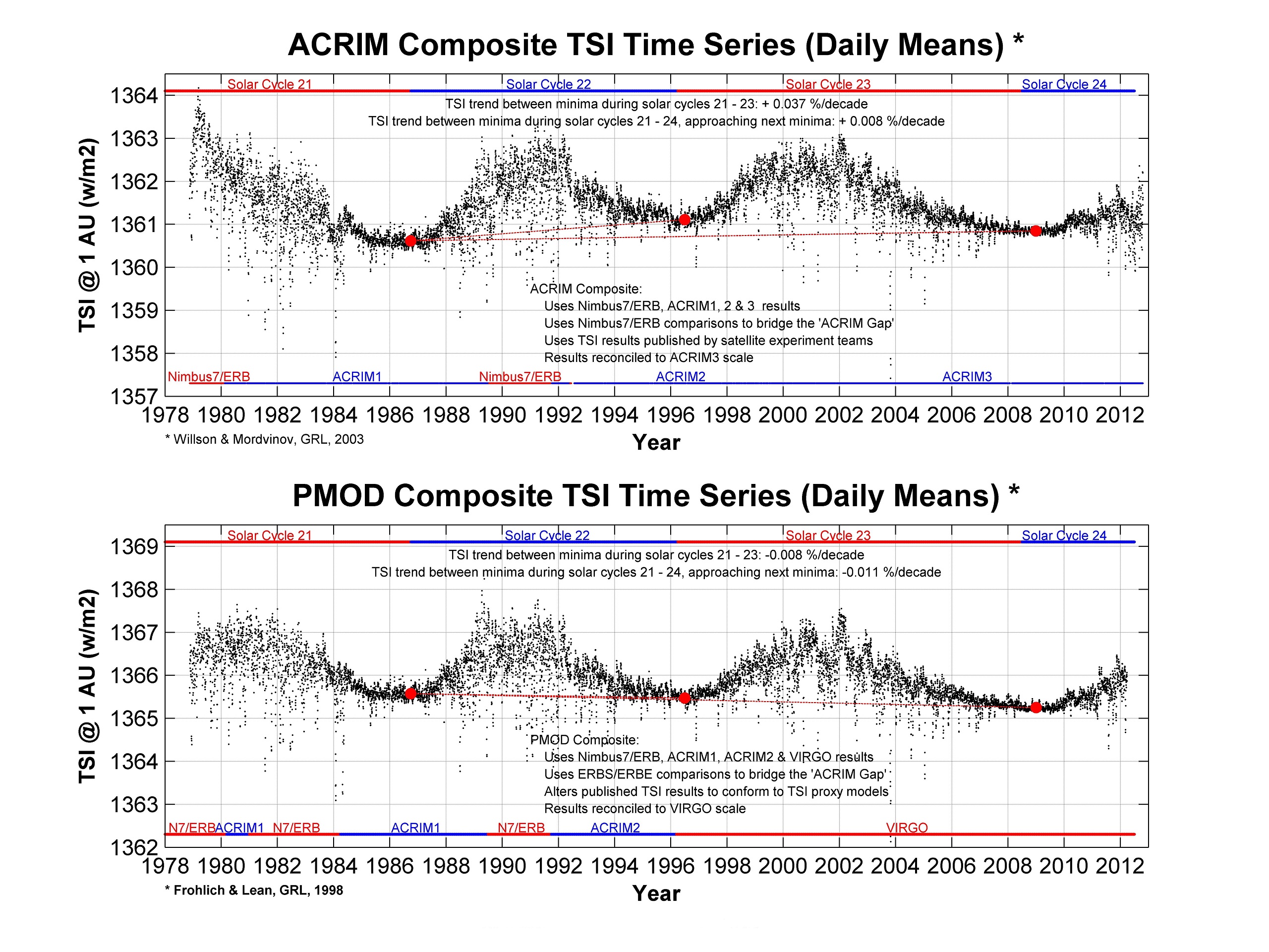
Figure 21: ACRIM (Willson and Mordvinov, 2003) and PMOD Fröhlich (2009) total solar irradiance satellite composites.

A serious source of uncertainty refers to the solar forcing functions that have to be used in the GCMs: see also Gray et al. (2010) for a general discussion on the topic. For example, CMIP5 GCMs used only a TSI forcing function deduced from Wang et al. (2005), but TSI functions are currently extremely uncertain (e.g.: Hoyt and Schatten, 1993; Lockwood, 2011; Shapiro et al., 2011). Using correct solar forcing functions in the GCMs is fundamental if the climate system is very sensitive to solar variations as the above studies suggest. Direct TSI satellite measurements started in 1978. However, an upward TSI trend from 1980 to 2000 followed by a decrease since 2000 is implied by the ACRIM TSI satellite composite (Willson and Mordvinov, 2003; Scafetta and Willson, 2009), which uses the TSI experimental data as published by the original science teams. An alternative TSI satellite composite, the PMOD, based on altered TSI data (Fröhlich, 2006, 2009), shows a gradual TSI decrease from 1980 to 2010. ACRIM and PMOD TSI satellite composites are compared in Figure 21. Before 1980 only highly controversial solar proxy reconstructions exist.

The CMIP5 GCMs use the recommended TSI proxy model prepared by Lean and collaborators (Wang et al., 2005; Kopp and Lean, 2011), which does not show a TSI increase from 1980 to 2000, presents a peak around 1960, as also shown by the sunspot number record, and presents a relatively small secular variability since the Maunder solar minimum of the 17th century. On the contrary, some alternative TSI reconstructions present a larger secular variability (Hoyt and Schatten, 1993, 1997), peak in the 1940s and in the 2000, and correlate with the GST records far better than Lean’s TSI proxy models (Loehle and Scafetta, 2011; Soon, 2005, 2009; Soon et al., 2011). Also solar cycle length models (Thejll and Lassen, 2000) peak in the 1940s instead of $\sim$1960. Schrijver et al. (2011), Shapiro et al. (2011) and Vieira et al. (2011) have recently proposed quite contrasting TSI reconstructions with a range of secular variability from very small to very large secular variability and significantly differ from Lean’s TSI models.

Figure 22A compares the latest Lean model (Kopp and Lean, 2011) and the model proposed by Hoyt and Schatten (1993). Figure 22B shows that the solar model proposed by Hoyt and Schatten (1993, 1997) well correlates with the central England temperature (CET) reconstruction (Parker et al., 1992) since 1700, suggesting a strong climate sensitivity to solar changes. Figure 22B suggests that the sun could have contributed about half of the 20th century warming in England: see Scafetta (2013a, b) for additional details. In any case, even if the proposed TSI reconstructions differ from each other in important details, there exists a general agreement that solar activity during the second half of the 20th century was higher than the previous centuries suggesting that the observed global warming since 1900 could have been partially caused by the increased solar activity (Scafetta and West, 2007; Scafetta, 2009a).

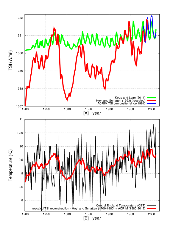
Figure 22: [A] Total solar irradiance (TSI) reconstruction by Hoyt and Schatten (1993) (red) rescaled on the updated ACRIM3 record (Willson and Mordvinov, 2003) (since 1981) (blue) vs. the updated Lean model (Wang et al., 2012; Kopp and Lean, 2011) (green). [B] Comparison between the Central England Temperature (CET) record (black) Parker et al. (1992) and the TSI model by Hoyt and Schatten merged with the ACRIM TSI record since 1981. Good correlation is observed at least since 1772.

Because the CMIP5 GCMs use Lean’s TSI model, it is also important to point out that despite serious controversy over the TSI dynamical behavior before 1992, the experimental TSI satellite groups (ACRIM and PMOD) agree that the TSI minimum in 1996 was higher than the TSI minimum in 2008 by at least 0.2-0.3 $W/m^{2}$: see ACRIM and PMOD TSI satellite composites at http://acrim.com/TSI%20Monitoring.htm). The open solar magnetic flux, the galactic cosmic ray (GCR) flux and other solar indexes also suggest that solar activity was higher in 1996 than in 2008 (Lockwood, 2012; Schrijver et al., 2011; Shapiro et al., 2011; Vieira et al., 2011). However, the updated Lean’s TSI proxy model (Kopp and Lean, 2011) fails to reproduce this pattern by predicting a 1996 TSI minimum (1360.7370 $W/m^{2}$) lower than the 2008 TSI minimum (1360.8217 $W/m^{2}$)
(http://lasp.colorado.edu/data/sorce/tsi_data/TSI_TIM_Reconstruction.txt).

Recently, Liu et al. (2013) used the ECHO-G model and showed that to reproduce the $\sim 0.7$ ${}^{o}C$ global cooling observed from the Medieval Warm Period (MWP: 900-1300) to the Little Ice Age (LIA: 1400-1800) according to recent paleoclimatic temperature reconstructions (e.g.: Christiansen and Ljungqvist, 2012; Ljungqvist, 2010; Mann et al., 2008; Moberg et al., 2005), a TSI model with a secular variability $\sim 3.5$ times larger than that shown by Lean’s TSI model would be required.

Thus, there is a realistic possibility that for their climatic simulations the current GCMs are not using sufficient solar-climate physical mechanisms and, by adopting Lean’s TSI model, are not even using a sufficiently accurate solar radiative forcing record. In the next section, an alternative solar model based on astronomical harmonic constituents will be used. This model is constructed adopting a very different methodology than those used to construct the above TSI proxy models. A strength of the proposed harmonic solar model is that it has been shown to hindcast quite well major solar and climate patterns during the Holocene (Scafetta, 2012c).

The author notes that Benestad and Schmidt (2009), using theoretical results derived from the GISS GCM simulations, criticized some of Scafetta’s preliminary studies (Scafetta and West, 2005, 2006) that demonstrated a significant solar contribution (up to 40-70%) to the 1850-2000 warming: they claimed that the sun contributed about 7% of the 20th century warming. However, GISS models do not reproduce the observed oscillations at multiple time scales (Scafetta, 2010, 2012b) and cannot be used to validate or contradict studies based on data analysis. Scafetta (2009a) confirmed his previous results with hindcast based models. Moreover, Benestad and Schmidt (2009)’s work also contains flawed models in particular with regard to use of linear regression algorithms and the wavelet decomposition algorithm (Scafetta, 2009b, 2013b). Linear regression algorithms are inefficient when the constructors are collinear, and during the 20th century the solar forcing is collinear with the anthropogenic forcing: both trend upward. Using linear regression algorithms in non-collinear situations Scafetta (2013b) showed: (1) GISS ModelE significantly underestimate the solar signature by a factor from 3 to 8; and (2) modern paleoclimatic temperature reconstructions imply that the sun contributed significantly to the 20th century warming. Moreover, Benestad and Schmidt (2009) used the periodic padding in the wavelet algorithm, which is highly inappropriate for decomposing trending sequences, instead of the reflection one, which minimizes Gibbs boundary artifacts. Figures 7 and 8 in Benestad and Schmidt (2009) demonstrate the mathematical error: the increased solar activity from the solar minimum in 1995 to the solar maximum in 2002 is claimed to have induced a significant cooling in the climate system, which would imply a nonphysical negative climate sensitivity to radiative forcing from 1995 to 2002. This is just a boundary artifact due to Benestad and Schmidt (2009)’s erroneous implementation of the wavelet algorithm: see Scafetta (2013b); Scafetta2013d for details.

In conclusion, the GCM implemented analytical approach cannot take into account unknown physical mechanisms and uncertain forcings. On the contrary, empirical modeling may reconstruct geometrical dynamical patterns, such as cycles, independently of their microscopic physical cause. It is important not to draw a logically flawed conclusion that a strong climatic response to solar/astronomical inputs does not exist simply because current GCMs are not able to reproduce it (Lockwood, 2012). Because of the existence of numerous physical uncertainties, it may be useful to investigate the possibility of an empirical methodology alternative to the analytical GCM one.

6 The astronomically-based empirical harmonic
model

In the following subsections I summarize a number of pieces of empirical evidence suggesting a significant climate sensitivity to astronomical/solar forcings. A semi-empirical harmonic constituent climate model is proposed. It is made of specific astronomical oscillations that can be used to simulate natural climatic variability. The proposed model outperforms all CMIP5 GCMs.

6.1 Millennial solar cycle, paleoclimatic temperature reconstructions, and their interpretation.

Understanding the natural variability of the climate of the past is necessary to properly interpret the climate changes occurred since 1850. If pre-industrial climate changes were similar to those observed since the industrialization period, natural variability might have been the major determinant of the present climatic changes. On the contrary, if the climatic changes that occurred since 1850 were anomalous relative to the preceding climate, this would support anthropogenic forcing as the major determinant of the 20th century global warming.

From 1998 to 2004 some preliminary studies claimed that the preindustrial GST since Medieval times varied very little, by about 0.2 ${}^{o}C$, while GST anomalously increased since 1900 (Mann et al., 1999; Mann and Jones, 2003): the shape of these proxy temperature reconstructions resembled that of an hockey stick with a MWP as warm as the 1900-1920 period. A number of climate model studies concluded that the solar radiative forcing plus volcanic and anthropogenic forcings were sufficient to explain those paleoclimatic GST records for the last millennium. This type of analysis led to the conclusion that the warming observed since 1900 could be due only to anthropogenic forcing (Crowley, 2000; Shindell et al., 2003; Hegerl et al., 2006; Fyfe et al., 2013).

Crowley (2000) explicitly stated: “The very good agreement between models and data in the preanthropogenic interval also enhances confidence in the overall ability of climate models to simulate temperature variability on the largest scales”, which suggests that in 2000 some climate scientists thought that the available climate models supporting the anthropogenic global warming theory for the 20th century were already sufficiently accurate (that is the science was considered sufficiently settled) because of their ability to hindcast the hockey stick GST proxy reconstructions. This interpretation was strongly advocated and promoted by the IPCC in 2001 and 2007 and greatly contributed to support the anthropogenic global warming theory and the GCMs that predicted it.

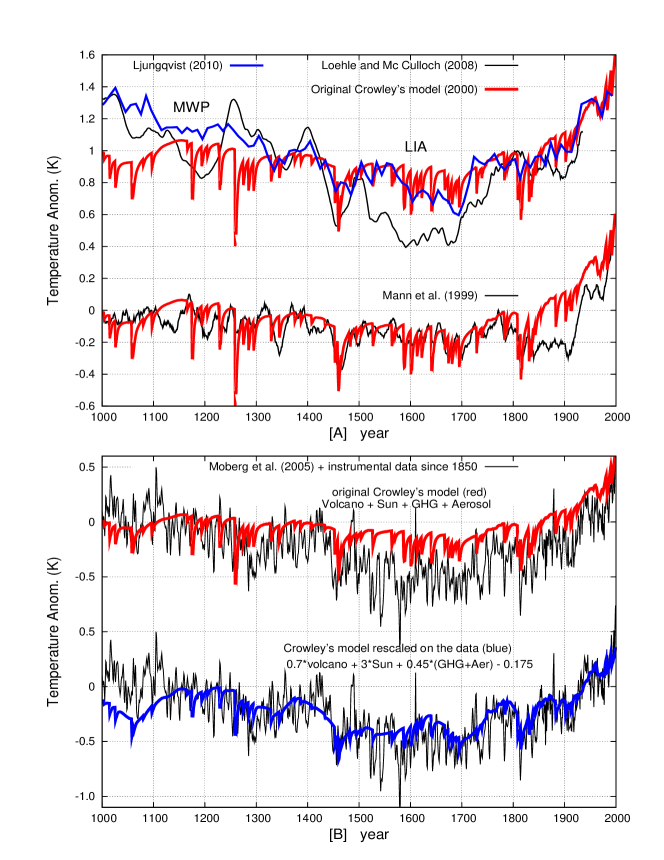
Figure 23: [A] Comparison between the original energy balance model prediction by Crowley (2000) versus the hockey stick temperature graph by Mann et al. (1999) implying a MWP as warm as the 1900-1920 period, and two non-hockey stick recent paleoclimate GST reconstructions (Loehle and Mc Culloch, 2008; Ljungqvist, 2010) showing a far larger preindustrial variability and a MWP as warm as the 1940-2000 period. [B](Bottom) the volcano, solar and GHG+Aerosol temperature signature components produced by Crowley (2000) model are scaled to fit (Moberg et al., 2005) paleoclimate GST reconstruction corrected since 1850 by HadCRUT4, which also shows a MWP as warm as the 1940-1970 period. See Scafetta (2013a, b) for more details.

However, since 2005 a number of studies have demonstrated a larger global pre-industrial temperature variability. For example, it was found a cooling of about 0.4-1.0 ${}^{o}C$ from the MWP to the LIA and a MWP as warm as the 1950-2000 period (Moberg et al., 2005; Mann et al., 2008; Loehle and Mc Culloch, 2008; Kobashi et al., 2010; Ljungqvist, 2010; McShane and Wyner, 2011; Christiansen and Ljungqvist, 2012). The new emerging millennial GST pattern stresses the existence of a large millennial climatic oscillation. A quasi millennial climatic oscillation is also found to correlate well with the millennial solar oscillation observed throughout the Holocene (Bond et al., 2001; Kerr, 2001; Ogurtsov et al., 2002; Kirkby, 2007; Steinhilber et al., 2012; Scafetta, 2012c).

The climate models that predicted a very small natural variability and that were used to fit the hockey stick temperature records can not fit the recent proxy GST reconstructions casting doubts on their accuracy. Still recent millennium simulation studies using modern solar models (that is, Wang et al., 2005) are able to predict only hockey-stick temperature graph showing an average cooling from the 900-1300 MWP to the 1300-1800 LIA up to $\sim$0.3 ${}^{o}C$, and just half of the empirically measured 11-year solar signature on the climate (see Feulner and Rahmstorf (2010) and IPCC (2007) figure 6.14: http:/www.ipcc.ch/publications_and_data/ar4/wg1/en/figure-6-14.html). These results are unsatisfactory, as also Liu et al. (2013) noted by demonstrating the need of assuming a far stronger solar effect to properly interpret the modern paleoclimatic temperature reconstructions.

For example, Ljungqvist (2010) and Christiansen and Ljungqvist (2012) estimations of the last 2000 years of extra-tropical Northern Hemisphere (30-90 ${}^{o}N$) decadal mean temperature variations present two large millennial cycles. These GST reconstructions claim that the Roman Maximum and the MWP were as warm as today’s temperatures. Indeed, these reconstructions might be quite plausible because they agree with inferences deduced from numerous historical documents (Guidoboni et al., 2011). For example, the medieval Vikings’ villages in Greenland clearly indicate a MWP warmer than today’s temperature at least in the North Atlantic (Esper et al., 2012; Surge and Barret, 2012). However, a medieval warm period does not appear to be limited to the Northern Atlantic region. Similar evidence exists also for China (Ge et al., 2003), South America (Neukom et al., 2011), South Africa (Tyson et al., 2000) the Indo-Pacific region (Oppo et al., 2009) and other locations (Soon and Baliunas, 2003). Thus, the MWP phenomenon was likely more global than was believed in 2000.

Figure 23 illustrates the paradigm-shift issue related to the current understanding of the historical climate. Figure 23A depicts the original climate model by Crowley (2000) against the temperature reconstruction by Mann et al. (1999) (note the good pre-1900 fit) and against two non hockey-stick temperature reconstructions (Loehle and Mc Culloch, 2008; Ljungqvist, 2010) (note the poor fit). Figure 23B depicts the temperature model by Moberg et al. (2005) (1000-1850) merged with the historical GST measurements since 1850 against the original climate model by Crowley (2000) (note the poor fit) and against an empirical model made by simply rescaling via linear regression the same climatic (solar, volcano and GHG+Aerosol) components predicted by Crowley’s model in such a way as to best fit the depicted temperature record (note the recovered overall good fit). The mathematical formula used in the regression model is reported in the figure: see Scafetta (2013a, b) for an extended discussion on this exercise.

The rescaled climate model indicates that for reproducing recent paleoclimate temperature reconstructions with their larger millennial GST cycle, the solar impact on the climate needs to be increased by at least a factor of three relative to the Crowley’s original estimate, which was already twice that predicted by the current CMIP3 GCM models: see Scafetta (2013b) for additional details. This also means that a significant fraction of the warming observed since 1900 (up to around 50% using different solar models) can be ascribed to the sun, as was calculated in Scafetta and West (2007) and Scafetta (2009a) using alternative methods. The volcano effect needs to be reduced by 30%, and the anthropogenic forcing effect (GHG plus Aerosol forcing) needs to be reduced by about 50%. The latter result well agrees with the correction implemented in Scafetta (2012b) that used an alternative reasoning based on the existence of a 60-year natural oscillation from 1970 to 2000 not modeled by the GCMs. The above finding also quantitatively confirms Eichler et al. (2009) and Zhou and Tung (2012), and contradicts the IPCC (2007), Benestad and Schmidt (2009) and Lean and Rind (2008), which claimed that 90% or more of the 20th century warming had to be caused by anthropogenic activity.

In conclusion, around 2000 hockey-stick shaped GST graphs implied a very small natural climatic variability (and a small solar effect) and a strong anthropogenic effect on climate. That evidence was consistent with the outputs of preliminary energy balance models, and is still consistent with the predictions of the CMIP3 and CMIP5 GCMs. However, recent paleoclimatic GST graphs have demonstrated a far larger preindustrial natural climate variability. The new evidence shifts the scientific paradigm. The climate should be highly sensitive to solar/astronomical related forcings because the novel GST reconstructions show a large millennial cycle that well correlates with solar/astronomical records (Bond et al., 2001; Kerr, 2001; Kirkby, 2007; Ogurtsov et al., 2002; Steinhilber et al., 2012). Consequently, the current GCMs should overestimate the anthropogenic effect on climate.

As also commented in Scafetta (2013a), Crowley (2000) and others would have had a significantly lower confidence in the overall ability of climate models to simulate temperature variability if in 2000 the current paleoclimatic temperature reconstructions had been available. The scientific community would have more likely concluded that important astronomically-related climate change mechanisms were still unknown, and needed to be investigated before they could be implemented to make reliable analytical GCMs.

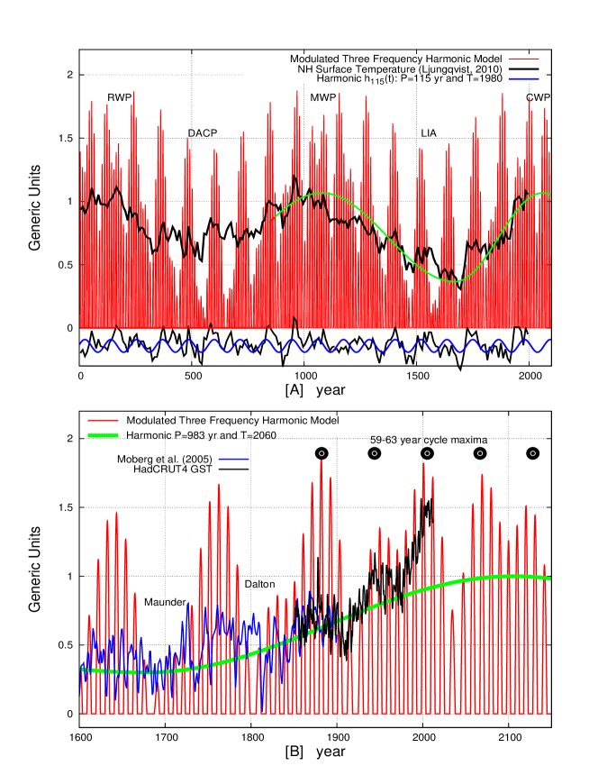
Figure 24: Scafetta (2012c) three-frequency solar model (red). [A] Against the Norther Hemisphere temperature reconstruction by Ljungqvist (2010) (black). The bottom depicts a filtering of the temperature reconstruction (black) that highlights the 115-year oscillation, $h_{115}(t)$, (blue). [B] The same solar model (red) is plotted against the HadCRUT4 GST (black) merged in 1850-1900 with the proxy temperature model by Moberg et al. (2005) (blue). The green curves highlight the quasi millennial oscillation, $h_{983}(t)$, with its skewness that approximately reproduces the millennial temperature oscillation. Note the hindcast of the Maunder and Dalton solar mimima and relative cool periods, and the projected quasi 61-year oscillation from 1850 to 2150. Adapted from Scafetta (2013a).

6.2 Construction of the astronomical/solar harmonics

Scafetta (2010, 2012a, 2012b) proposed that the quasi 60-year GST oscillation observed during 1850-2012, which has an amplitude of about 0.3 ${}^{o}C$ (see also Figure 2A), could indicate that about 50% of the 0.5 ${}^{o}C$ warming observed from 1970 to 2000 could have been due to this natural oscillation during its warming phase. Zhou and Tung (2012) reached a similar result using the Atlantic Multidecadal Oscillation, which also presents a clear quasi 60-year oscillation (e.g.: Mörner, 1989, 1990; Manzi et al., 2012), as a constituent regression model component to reconstruct the GST record.

The existence of a large natural oscillation causing about 50% of the 1970-2000 warming would mean that the net anthropogenic effect on the climate has been overestimated by the GCMs by at least the same percentage, and needs to be reduced on average by about a 0.5 factor, as alternatively demonstrated above (Section 6.1) using an approach based on recent paleoclimate temperature records. Consequently, also a significant fraction of the 1850-2013 warming (about 0.40-0.45 ${}^{o}C$) could not be reconstructed by the same GCMs. Note that part of the residual warming could also be due to poorly corrected urban heat island (UHI) and land use change (LUC) effects (McKitrick and Michaels, 2007; McKitrick and Nierenberg, 2010; Loehle and Scafetta, 2011). Thus, a reduction to a 0.5 factor of the output of the GCMs may be considered an upper limit. However, herein such a hypothesis is not taken into consideration and the GST records are assumed to show true climatic changes.

Figures 1 and 2 and Eq. 1-4 proposed a possible astronomical origin of the decadal and multidecadal GST oscillations. Interestingly, natural climatic oscillations linked to astronomical cycles with multidecadal periods of about 20 and 60 years, and longer secular and quasi-millennial cycles appear to have been well-known in ancient times, and in the Middle Ages through the Renascence. These astronomical oscillations could be easily deduced from the conjunction periods of Jupiter and Saturn and from their dynamical rotation along the Zodiac. These oscillations were included, for example, in Chinese and Indian calendars and constituted the basis for a kind of astrological climatology. Indeed, these oscillations could be observed in climate records, e.g. in the monsoon oscillations, and inferred from historical chronologies describing the fall and rise of human civilizations (Ptolemy, 2nd century; Ma’sǎr, 886; Kepler, 1601; Iyengar, 2009): see more details about the ancient understanding of climate changes in Scafetta (2013a).

A link between planetary oscillations and climatic cycles could be indirect. Planetary oscillations may modulate solar changes that then induce climatic changes. Indeed, Scafetta (2012c) analyzed in details the sunspot number record and noted that the 11-year Schwabe sunspot cycle is made of at least three harmonics interfering together at about 9.93 years, 10.87 years, and 11.86 years. The harmonic at 9.93 years corresponds to the Jupiter/Saturn spring tidal period and the 11.86 year corresponds to the Jupiter orbital period. The central period at 10.87 years could be generated by the solar dynamo itself by means of a dynamical synchronization process with the other two cycles or by a combination of the recurrent tidal cycles produced by Venus, Earth and Jupiter that present peaks at about 10.4 and 11.1 years. This finding suggests a planetary modulation of solar activity, as first proposed by Wolf (1859), whose physical mechanisms and additional empirical evidences are extensively discussed in a number of publications (Abreu et al., 2012; Brown, 1900; Fairbridge and Shirley, 1987; Hung, 2007; Landscheidt, 1999; Wolff and Patrone, 2010; Scafetta, 2010, 2012a, 2012c, 2012d; Scafetta and Willson, 2013a, b).

In particular Scafetta (2012d) argued that the Sun might be working as a huge amplifier of planetary gravitational oscillations because the planetary tidal work released to the sun, although quite small, could nevertheless be greatly amplified up to a 4 million factor by triggering a modulation of the core nuclear fusion rate. Electromagnetic planet-sun interactions can also be hypothesized (Scafetta and Willson, 2013a, b). Preliminary calculations suggests that Scafetta’s model could produce luminosity oscillations up to one order of magnitude compatible with the observed TSI oscillation. Such signal could be sufficiently powerful to modulate the solar dynamo mechanisms and produce a final TSI output approximately synchronized to planetary harmonics.

The three harmonics at 9.93 years, 10.87 years, and 11.86 years beat together forming a complex dynamics as shown in Figure 24 (red curve). Four major additional multidecadal, secular and millennial solar/astronomical oscillations emerge: a quasi 61-year oscillation (maximum around 2002), a 115-year oscillation (maximum around 1980) and a minor 130-year oscillation (maximum around 2035), and a large quasi 983-year oscillation (maximum around 2060). The beats of Scafetta (2012c) three-frequency model well correlate with the observed major solar and climatic variations for millennia, throughout the Holocene: see also Figure 24 and the extended discussion in Scafetta (2012c).

A 115-year oscillation can be observed in proxy temperature models going back for 2000 years (e.g.: Ogurtsov et al., 2002; Qian and Lu, 2010), and can be correlated with grand-solar minima such as the Maunder, Dalton and the solar minimum around 1910 and other grand solar minima during the last 1000 years. The 115-year oscillation is projected to reach a minimum in 2030-2040. Figure 24A suggests that this oscillations may be characterized by a temperature variation between 0.05 and 0.15 ${}^{o}C$. This cycle can be approximated as

$$h_{115}(t)=0.05\cos(2\pi(t-1980)/115).$$ (11)

A great millennial oscillation is observed throughout the Holocene (Bond et al., 2001; Kerr, 2001; Ogurtsov et al., 2002; Kirkby, 2007; Steinhilber et al., 2012; Scafetta, 2012c) and was responsible for the Roman Warm Period, the Dark Age Cold Period, the Medieval Warm Period, the Little Ice Age and the Current Warm Period, and would peak around 2060: see Figure 24A. As evident from poleoclimatic temperature proxy models, the millennial oscillation is skewed by other multisecular harmonics with a likely minimum around 1680 during the Maunder Solar Minimum: see also Humlum et al. (2011) and Figures 23 and 24. Assuming that the millennial temperature oscillation presents a variation of about $0.7\pm 0.3$ ${}^{o}C$, as approximately shown in Ljungqvist (2010) and in Moberg et al. (2005) (see Figures 23 and 24), it may be approximately modeled from 1680 to 2060 as

$$h_{983}(t)=0.35\cos(2\pi(t-2060)/760),$$ (12)

where the adoption of the shorter period of 760 years takes into account the skewness of the millennial cycle with a minimum in the middle of the Maunder solar minimum around 1680 and a predicted maximum in 2060. Note that if the cloud system is modulated by these solar/astronomical cycles, the GST could be modulated by these oscillations relatively quickly with a time lags spanning from a few months to just a few years as the frequency decreases (Scafetta, 2008, 2009a).

Figure 24A shows the proposed solar model versus the extra-tropical Norther Hemisphere temperature reconstruction by Ljungqvist (2010) (black). Note the two synchronous quasi millennial cycles and the common 115-year oscillation modulation, which is also highlighted at the bottom of the figure with an appropriate filtering of the temperature record. The blue curve at the bottom is the function $h_{115}(t)$. The figure highlights also the Roman Warm period (RWP), Dark Ages Cold Period (DACP), Medieval Warm Period (MWP), Little Ice Age (LIA) and Current Warm Period (CWP). Figure 24B depicts the solar model (red) versus HadCRUT4 (annual smooth: black) merged in 1850-1900 with the proxy temperature model by Moberg et al. (2005) (blue). Note the synchronous occurrence of both the colder periods during the Maunder and Dalton modeled solar minima, and the quasi 61-year modulation from 1850 to 2010. The solar model predicts a $\sim$61-year oscillation from 1850 to 2150 whose maxima are highlighted by the black circles. Before 1850, the 61-oscillation weakens. The Sun may be entering into a (minor) grand minimum centered in the 2030s. Indeed, sunspot cycles 19-23 (1955-2008) resemble sunspot cycles 1-4 (1755-1798) that preceded the Dalton solar minimum (1790-1830), and sunspot cycle 24 (2008-2021?) is approximately replicating the low sunspot cycle 5 (Scafetta, 2012c, Fig. 10). The millennial modulation, $h_{983}(t)$, is also highlighted in the figure (green).

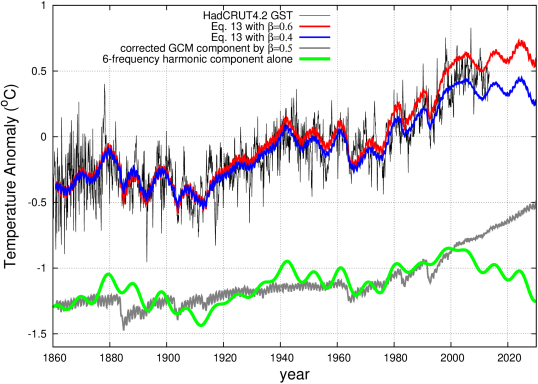
Figure 25: The semi-empirical model, Eq. 13, using $\beta=0.4$ (blue) and $\beta=0.6$ (red) attenuation of the CMIP5 ensemble mean simulation vs. HadCRUT4 GST record since 1860. The upward warming trending and all decadal and multidecadal patterns are well reconstructed. The bottom depicts the 6-frequency harmonic component that models the harmonic natural variability (green) and the GCM radiative component corrected by $\beta=0.5$ (grey), respectively.

6.3 The six-harmonic astronomical/solar model for climate change

With the above information a first approximation six-harmonic astronomical/solar model for climate change can be constructed, which phenomenologically simulates the corresponding natural oscillations that the GCMs are currently not able to reproduced. The additional radiative forcing component (e.g. GHG, aerosol, volcano effects) can to a first approximation be simulated by using the CMIP5 mean projections reduced by a given factor $\beta$. Thus, the semi-empirical model is given by the equation:

$$\begin{split}H(t)=h_{983}(t)+h_{115}(t)+h_{60}(t)+h_{20}(t)+h_{10.4}(t)\\ +h_{9.1}(t)+\beta*m(t)+const,\end{split}$$ (13)

where the function $m(t)$ is a CMIP5 ensemble mean simulation depicted in Figure 2.

Figure 25 shows that to reproduce accurately the HadCRUT4 GST warming trend since 1850 it is necessary to use $\beta=0.5\pm 0.1$. This result is reasonably compatible with that found in Scafetta (2012b) where a value of $\beta=0.45\pm 0.05$ was chosen using the CMIP3 models and the HadCRUT3 GST, with a slight lower secular global warming than the HadCRUT4 GST record. Scafetta (2012b) determined the coefficient $\beta$ only using an argument based on the GST residual from the harmonic model during the period 1970-2000. Indeed, because from 1970 to 2000 the HadCRUT4 GST warms a little bit more than the HadCRUT3 record, the same argument used in Scafetta (2012b) but applied to the HadCRUT4 record yields $\beta\approx 0.5$. The fact that with $\beta=0.5$ Eq. 13 simultaneously reconstructs both the 1970-2000 calibrating period and the entire 1850-2013 period validates the model with a hindcast test.

The result implies that the climate sensitivity to radiative forcing has been overestimated by the CMIP5 GCMs by about a factor of 2. Thus, the climate sensitivity to $CO_{2}$ doubling should be reduced from the IPCC (2007) claimed 2.0-4.5 ${}^{o}C$ range to a 1.0-2.3 ${}^{o}C$ range with a likely median of $\sim 1.5$ ${}^{o}C$ instead of $\sim 3.0$ ${}^{o}C$.

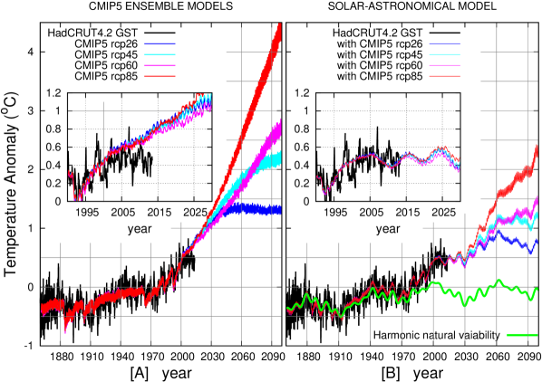
Figure 26: [A] The four CMIP5 ensemble average projections versus the HadCRUT4 GST record. [B] The solar-astronomical semi-empirical model, Eq. 13 with $\beta=0.5$, against the HadCRUT4 GST record: a common 1900-2000 baseline is used. The figure highlights the better performance of the solar-astronomical semi-empirical model versus the CMIP5 models, which is particularly evident since 2000 as shown in the inserts.

A reduction by about half of the climate sensitivity to radiative forcing is compatible with the results discussed in the subsection 6.1 and shown in Figure 23B concerning the interpretation of modern paleoclimatic temperature reconstructions with a larger pre-industrial variability with a MWP as warm as the 1950-2000 period. The result is also consistent with those by Chylek and Lohmann (2008) who found a climate sensitivity between 1.3 ${}^{o}C$ and 2.3 ${}^{o}C$ due to doubling of atmospheric concentration of $CO_{2}$, by Ring et al. (2012) who found a climate sensitivity in the range from about 1.5 ${}^{o}C$ to 2.0 ${}^{o}C$, and by Lewis (2013) who found a climate sensitivity range from 1.2 ${}^{o}C$ to 2.2 ${}^{o}C$ (median 1.6 ${}^{o}C$). The result is also consistent with Zhou and Tung (2012) and Chylek et al. (2013), who found that the anthropogenic warming has been overestimated by about a factor of 2.

The quasi 60-year harmonic component of the model may be sufficiently valid for the period 1880-2150 because Scafetta (2012c) three-frequency solar model predicts that during this period the major natural patterns in the solar dynamics may be described by a quasi 60-year oscillation slightly modulated by the 115-year oscillation, while the millennial oscillation is at its maximum.

The author notes that the CMIP5 models contain also a solar signature, but it is very small because the CMIP5 adopted TSI (Wang et al., 2005) has a smaller secular trend than the TSI records adopted for the CMIP3 GCMs in the IPCC (2007). Herein, this correction is ignored because within the 20% error associated to the $\beta=0.5$ factor, although the presence of a solar signature in $m(t)$ may slightly amplify the decadal cycle in $H(t)$. Note that Eq. 13 is not optimized for periods before 1850 because no GST are available before 1850, and the climate response to the deep grand solar minima (Dalton, Maunder etc.) could necessitate additional frequencies such as a 80-90 year oscillation (Scafetta and Willson, 2013a) and probably the inclusion of nonlinear dynamical effect. The 80-90 year cycle modulates the  60 year cycle by producing a beat with a period of  210 years known as the Suess (a.k.a. de Vries) solar cycle.

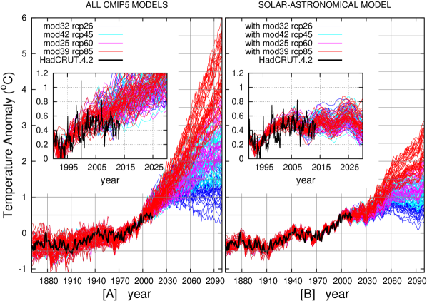
Figure 27: [A] All CMIP5 model projections versus the HadCRUT4 GST record. [B] The solar-astronomical semi-empirical model, Eq. 13 with $\beta=0.5$ , against the HadCRUT4 GST record: a common 1980-2000 baseline and annually resolved records are used in the large figures while the monthly GST record is used in the inserts. The figure highlights the better performance of the solar-astronomical semi-empirical model versus the CMIP5 models.

Figure 26 compares the four CMIP5 ensemble average projections (panel A) and the solar-astronomical semi-empirical model using $\beta=0.5$ in Eq. 13 (panel B) against the HadCRUT4 GST record: a common 1900-2000 baseline is used. The figure highlights the superior performance of the solar-astronomical semi-empirical model versus the CMIP5 ensemble mean models. Eq. 13 reconstructs all major decadal and multidecadal temperature patterns observed since 1860. The temperature plateau observed since 2000 is better reconstructed by the semi-empirical model than by the GCM mean projections. Thus, the 2000-2013 GST plateau appears to be due to the cooling phase of a natural quasi 60-year oscillation that has balanced a strongly reduced projected anthropogenic warming trend. The four adopted CMIP5 GCM mean projections display a 2000-2100 warming between a minimum of about 1 ${}^{o}C$ to a maximum of about 4 ${}^{o}C$ (see figure 26A). However, as Figure 26B shows, the four corrected projections predict a 2000-2100 warming between a minimum of about 0.3 ${}^{o}C$ to a maximum of about 1.8 ${}^{o}C$ using the same anthropogenic scenarios. The inserts magnify the period 1990-2030 to highlight the strong mismatch between the GST and the GCM simulations since 2000 that is resolved with the solar-astronomical semi-empirical model.

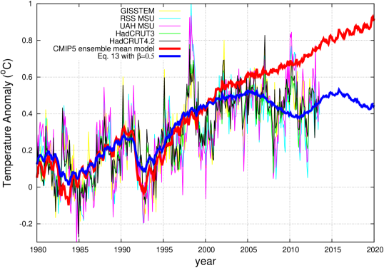
Figure 28: Eq. 13 with $\beta=0.5$ (blue) and the original CMIP5 ensemble mean model (red) against six global temperature estimates (HadCRUT3, HadCRUT4, UAH MSU, RSS MSU, GISS and NCDC), which were base-lined with HadCRUT4 from Jan/1980 to Dec/1999. Temperature data from: http://www.ncdc.noaa.gov, http://www.metoffice.gov.uk, http://data.giss.nasa.gov, http://www.remss.com/, http://vortex.nsstc.uah.edu/

Figure 27 is similar to Figure 26 but with all CMIP5 model individual simulations used in Eq. 13 with $\beta=0.5$. Again, the figure highlights the superior performance of the solar-astronomical semi-empirical model versus the CMIP5 model simulations. The solar-astronomical semi-empirical model also causes a reduction of the range among the simulation by a factor of two. The root-mean-square deviation (RMSD) value between the 49-month average smooth GST and the full empirical model is about 0.04 ${}^{o}C$, while for the RMSD for the GCM model mean is twice, 0.09 ${}^{o}C$, and for the single GCM runs is normally larger (see Table 2).

Figure 28 magnifies the period 1980-2020 and uses six global temperature estimates (HadCRUT3, HadCRUT4, UAH MSU, RSS MSU, GISS and NCDC) that appear to agree sufficiently well with each other and all of them disagree with the CMIP5 simulations after 2000. The temperature may slightly increase from 2013 to 2016, and decrease from 2016 to 2020 because of the two decadal cycles. However, fast ENSO temperature fluctuations at scales shorter than 7 years may mask the result.

In conclusion, because the temperature patterns appears well correlated with solar/astronomical oscillations at multiple scales and that semi-empirical models based on these oscillations reconstruct and hindcast GST variations significantly better than the current GCMs, it is very likely that the observed GST oscillations have an astronomical origin whose mechanisms are not implemented in the GCMs yet. To better appreciate the finding, it is important to stress that the harmonic constituents of the proposed model, such as the frequencies and the phases, are coherent with major astronomical oscillations. Although in the future the empirical model may be improved with a better understanding of these oscillations, the proposed semi-empirical model already appears to outperform all CMIP5 GCMs.

7 Conclusion

As for the CMIP3 GCMs used by the IPCC 2007 (Scafetta, 2012b), the upgraded CMIP5 GCMs to be used in the IPCC Fifth Assessment Report (AR5, 2013) do not reproduce the detectable decadal and multidecadal climate oscillations observed in the GST records since 1850. Multiple analyses suggest that these GCMs overestimate the anthropogenic warming effect by about 50%. This would also imply that the climate sensitivity to the radiative forcing should be significantly lowered by half. It may be $\sim 1.5$ ${}^{o}C$ (or less if part of the warming is spurious, for example due to uncorrected UHI effects), and it may possibly range between 1 ${}^{o}C$ and 2.3 ${}^{o}C$ instead of the IPCC (2007) proposed range from 2 ${}^{o}C$ to 4.5 ${}^{o}C$. Very important physical mechanisms necessary for reproducing multiple climatic oscillations, which are responsible for about half of the 1850-2010 warming appear to be still missing in the GCMs.

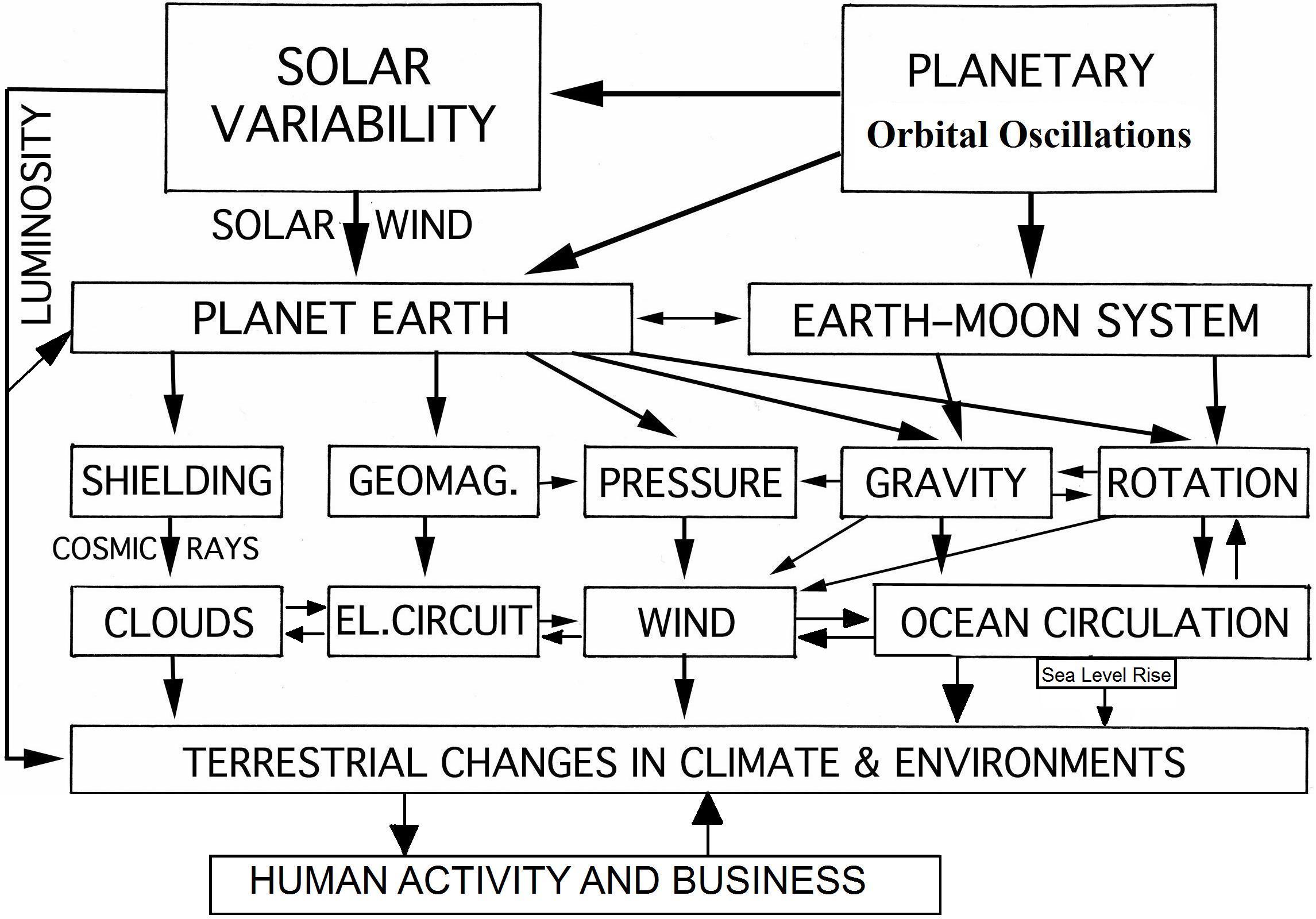
Figure 29: Network of the possible physical interaction between planetary harmonics, solar variability and climate and environments changes on planet Earth (adapted with permission after Mörner (2012), see also Scafetta (2013b)).

The physical origin of the detected climatic oscillations is currently uncertain, but in this paper it has been argued that they may be astronomically induced. This conclusion derives from the coherence found among astronomical and climate oscillations from the decadal to the millennial time scales. This harmonic component cannot be ignored in properly interpreting and forecasting climate change. I have shown that an empirical model based on specific major astronomical harmonics plus a correction of the outputs of the current CMIP5 GCM simulations simultaneously reconstructs the decadal, multidecadal and secular patterns observed in the GST records since 1850.

The most reasonable conclusion is that the climate system is synchronized to the natural oscillations found in the solar system and that this harmonic dynamics constitutes an important component of the Earth’s climate. The proposed semi-empirical model may produce more reliable projections for the 21st century, which are far less alarmist than the current CMIP5 projections. Under the same anthropogenic emission scenarios, the model projects a possible 2000-2100 warming ranging from 0.3 ${}^{o}C$ to 1.8 ${}^{o}C$. This range is significantly below the original CMIP5 GCM ensemble mean projections spanning from about 1 ${}^{o}C$ to 4 ${}^{o}C$.

In conclusion, multiple statistical tests suggest that the proposed semi-empirical GST model based on astronomically induced harmonics plus an anthropogenic plus volcano contribution reduced by about 50% from the CMIP5 GCM prediction outperforms all CMIP5 GCMs in reconstructing and interpreting the GST patterns observed since 1850. The model would be compatible also with modern paleoclimatic reconstructions showing a larger pre-industrial variability with a medieval period as warm as the 1950-2000 global surface temperatures.

Future research should investigate space-climate coupling mechanisms in order to develop more advanced analytical and semi-empirical climate models. Figure 29 schematically represents a possible network of physical interactions causing climatic changes.

Appendix

The proposed harmonic model, Eq. 13, uses a specific set of harmonics first determined in Scafetta (2010). Scafetta (2013a) also proposed a model with slightly different decadal and multidecadal frequencies: harmonics with period of 10.2 years, 21 years and 61 years were used instead of harmonics with period of 10.4 years, 20 years, and 60 years. Scafetta (2013a) choice was justified by spectral analysis results and by the possibility that the observed harmonics could be induced by multiple closed astronomical frequencies with a different physical origin.

For example, the quasi 20-year GST oscillation could be induced by a combination of the 18.6-year lunar nutation cycle, of the 19.85-year oscillation of the speed of the wobbling sun related to the conjunction of Jupiter and Saturn and of the quasi 22-year Hale solar magnetic cycle. Indeed, Chylek et al. (2011) found evidence in multisecular ice-core data for a prominent near 20-year time-scale oscillation that beats and appears to be composed of three close frequencies. Similarly, the quasi 60-year GST oscillation could be caused by the 59.6 years cycle in the speed of the wobbling sun and by the 61-year tidal beat between Jupiter orbit (11.86 years) and Jupiter and Saturn’s spring tide (9.93 years). It is evident that if the planets are modulating solar activity and, directly or indirectly, the climate of the Earth, numerous harmonics may be involved in the process, as also found in Scafetta and Willson (2013a, b).

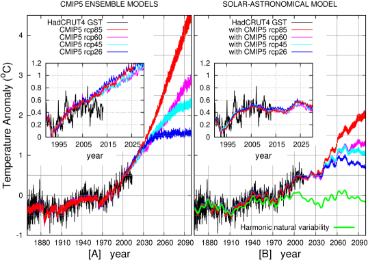
Figure 30: Reproduction of Figure 26 with the alternative model and data proposed in Scafetta (2013a) that uses slight different decadal and multidecadal harmonics.

By analogy, the harmonic constituent model currently used to predict the ocean tides (Kelvin, 1881; Ehret, 2008) uses 30-40 harmonics whose frequencies are deduced from the orbits of the sun and of the moon. Many of the tidal harmonics are closely clustered (see http://en.wikipedia.org/wiki/Theory_of_tides#Tidal_constituents). For example, the semi-diurnal tidal oscillation is modeled using 8 frequencies spanning from 11.6 h (the shallow water semidiurnal cycle) to 12.9 h (the lunar elliptical semidiurnal second-order cycle).

Thus, the proposed harmonic model, Eq. 13, which is based on a choice of just six harmonics spanning from the decadal to the millennial scales should be interpreted as a minimal first approximation model. Future research should better define the true physical harmonics involved in the process which may be numerous. In any case, from a practical point of view the alternative model proposed in Scafetta (2013a) produces similar results to Eq. 13, as shown in Figure 30 that reproduces Figure 26 with the alternative model and data.

References

Table 2: See Section 3.1. The regression coefficients are evaluated using Eq. 7 for all available 162 GCM simulations and for their ensemble mean (which is numbered -0- in the list). The table reports the $\chi^{2}$ test values, which were calculated using Eq. 13, and the root-mean-square deviation (RMSD) values for each simulations from the harmonic model Eq. 6, which were calculated using a 49-month running mean of the original time sequences. See also Figure 12.

#	Model	Simulation	$\alpha$	$\alpha$	$\alpha$	$\alpha$	$\beta$	$\gamma$	$\chi^{2}$	RMSD
		#	(60-years)	(20-years)	(10.4=years)	(9.1-years)	(upward trend)	(bias)
	GST		1 $\pm$ 0.05	1 $\pm$ 0.12	1 $\pm$ 0.17	1 $\pm$ 0.11	1 $\pm$ 0.02	0.0 $\pm$ 0.01	0	0.05
0	GCM mean		0.63 $\pm$ 0.03	0.73 $\pm$ 0.08	0.44 $\pm$ 0.12	0.40 $\pm$ 0.08	1.04 $\pm$ 0.01	-0.55 $\pm$ 0.00	14.3	0.09
1	ACCESS1-0	0	0.39 $\pm$ 0.05	0.92 $\pm$ 0.14	0.88 $\pm$ 0.20	0.70 $\pm$ 0.13	0.84 $\pm$ 0.02	0.12 $\pm$ 0.01	21.4	0.14
2	ACCESS1-3	0	0.46 $\pm$ 0.05	0.89 $\pm$ 0.12	1.05 $\pm$ 0.17	0.02 $\pm$ 0.12	0.58 $\pm$ 0.02	0.08 $\pm$ 0.00	69.4	0.14
3		1	0.67 $\pm$ 0.05	0.81 $\pm$ 0.12	0.23 $\pm$ 0.17	-0.07 $\pm$ 0.12	0.51 $\pm$ 0.02	0.07 $\pm$ 0.00	81.7	0.15
4		2	0.75 $\pm$ 0.04	1.33 $\pm$ 0.11	0.08 $\pm$ 0.16	-0.03 $\pm$ 0.11	0.39 $\pm$ 0.02	0.06 $\pm$ 0.00	123.6	0.15
5	bcc-csm1-1	0	1.29 $\pm$ 0.05	0.62 $\pm$ 0.14	0.19 $\pm$ 0.19	0.55 $\pm$ 0.13	1.42 $\pm$ 0.02	0.17 $\pm$ 0.01	51.4	0.14
6		1	0.64 $\pm$ 0.06	0.41 $\pm$ 0.14	0.59 $\pm$ 0.20	1.03 $\pm$ 0.14	1.72 $\pm$ 0.02	0.22 $\pm$ 0.01	129.9	0.19
7		2	0.77 $\pm$ 0.06	0.69 $\pm$ 0.15	0.60 $\pm$ 0.22	0.57 $\pm$ 0.15	1.50 $\pm$ 0.02	0.19 $\pm$ 0.01	58.3	0.17
8	bcc-csm1-1-m	0	0.40 $\pm$ 0.06	0.83 $\pm$ 0.15	0.81 $\pm$ 0.22	0.48 $\pm$ 0.15	1.44 $\pm$ 0.02	0.20 $\pm$ 0.01	55.7	0.16
9		1	0.31 $\pm$ 0.07	0.73 $\pm$ 0.17	1.19 $\pm$ 0.25	1.09 $\pm$ 0.17	1.46 $\pm$ 0.03	0.18 $\pm$ 0.01	54.1	0.18
10		2	0.25 $\pm$ 0.07	1.07 $\pm$ 0.19	0.68 $\pm$ 0.26	1.01 $\pm$ 0.18	1.65 $\pm$ 0.03	0.23 $\pm$ 0.01	86.6	0.22
11	BNU-ESM	0	0.82 $\pm$ 0.06	1.12 $\pm$ 0.16	0.19 $\pm$ 0.23	-0.18 $\pm$ 0.16	1.78 $\pm$ 0.02	0.27 $\pm$ 0.01	131.5	0.20
12	CanESM2	0	0.88 $\pm$ 0.07	0.85 $\pm$ 0.17	0.14 $\pm$ 0.24	0.04 $\pm$ 0.17	1.17 $\pm$ 0.03	0.17 $\pm$ 0.01	12.3	0.15
13		1	1.17 $\pm$ 0.06	1.39 $\pm$ 0.16	0.51 $\pm$ 0.23	0.66 $\pm$ 0.15	1.05 $\pm$ 0.02	0.15 $\pm$ 0.01	3.5	0.13
14		2	0.89 $\pm$ 0.06	0.48 $\pm$ 0.16	0.60 $\pm$ 0.22	0.83 $\pm$ 0.15	1.10 $\pm$ 0.02	0.16 $\pm$ 0.01	4.5	0.13
15		3	0.85 $\pm$ 0.06	1.00 $\pm$ 0.16	0.78 $\pm$ 0.22	-0.22 $\pm$ 0.15	1.16 $\pm$ 0.02	0.17 $\pm$ 0.01	14.6	0.13
16		4	1.17 $\pm$ 0.06	1.20 $\pm$ 0.16	1.11 $\pm$ 0.23	0.11 $\pm$ 0.15	1.19 $\pm$ 0.02	0.17 $\pm$ 0.01	12.7	0.14
17	CCSM4	0	0.74 $\pm$ 0.06	0.75 $\pm$ 0.15	1.03 $\pm$ 0.22	0.13 $\pm$ 0.15	1.58 $\pm$ 0.02	0.24 $\pm$ 0.01	81.5	0.17
18		1	0.74 $\pm$ 0.05	0.68 $\pm$ 0.14	-0.02 $\pm$ 0.20	0.47 $\pm$ 0.13	1.64 $\pm$ 0.02	0.25 $\pm$ 0.01	107.7	0.16
19		2	0.63 $\pm$ 0.06	0.27 $\pm$ 0.15	0.83 $\pm$ 0.21	0.82 $\pm$ 0.14	1.55 $\pm$ 0.02	0.24 $\pm$ 0.01	78.0	0.15
20		3	0.59 $\pm$ 0.06	0.60 $\pm$ 0.15	-0.06 $\pm$ 0.22	0.98 $\pm$ 0.15	1.59 $\pm$ 0.02	0.24 $\pm$ 0.01	85.4	0.17
21		4	0.58 $\pm$ 0.06	0.45 $\pm$ 0.15	0.73 $\pm$ 0.21	0.28 $\pm$ 0.14	1.60 $\pm$ 0.02	0.24 $\pm$ 0.01	92.8	0.17
22		5	0.56 $\pm$ 0.05	1.16 $\pm$ 0.14	0.83 $\pm$ 0.20	0.75 $\pm$ 0.14	1.59 $\pm$ 0.02	0.25 $\pm$ 0.01	92.6	0.16
23	CESM1-BGC	0	0.67 $\pm$ 0.05	0.45 $\pm$ 0.14	1.09 $\pm$ 0.20	1.07 $\pm$ 0.14	1.50 $\pm$ 0.02	0.23 $\pm$ 0.01	64.6	0.15
24	CESM1-CAM5	0	0.29 $\pm$ 0.05	0.66 $\pm$ 0.12	0.30 $\pm$ 0.17	0.78 $\pm$ 0.12	0.88 $\pm$ 0.02	0.13 $\pm$ 0.00	27.9	0.11
25		1	1.01 $\pm$ 0.05	1.01 $\pm$ 0.12	0.80 $\pm$ 0.17	0.58 $\pm$ 0.12	0.79 $\pm$ 0.02	0.11 $\pm$ 0.00	13.7	0.10
26		2	0.99 $\pm$ 0.05	0.55 $\pm$ 0.13	1.41 $\pm$ 0.18	0.48 $\pm$ 0.12	0.92 $\pm$ 0.02	0.13 $\pm$ 0.00	5.7	0.10
27	CESM1-CAM5-1-FV2	0	0.87 $\pm$ 0.06	0.04 $\pm$ 0.16	1.32 $\pm$ 0.23	0.63 $\pm$ 0.16	0.71 $\pm$ 0.02	0.09 $\pm$ 0.01	22.2	0.15
28		1	1.05 $\pm$ 0.06	0.34 $\pm$ 0.14	1.48 $\pm$ 0.20	0.08 $\pm$ 0.14	0.72 $\pm$ 0.02	0.10 $\pm$ 0.01	27.1	0.11
29		2	0.77 $\pm$ 0.05	-0.08 $\pm$ 0.14	0.11 $\pm$ 0.20	-0.05 $\pm$ 0.14	0.85 $\pm$ 0.02	0.12 $\pm$ 0.01	23.8	0.11
30		3	0.61 $\pm$ 0.06	0.64 $\pm$ 0.16	-0.06 $\pm$ 0.22	0.16 $\pm$ 0.15	0.81 $\pm$ 0.02	0.11 $\pm$ 0.01	20.3	0.13
31	CESM1-FASTCHEM	0	0.62 $\pm$ 0.06	0.79 $\pm$ 0.15	0.25 $\pm$ 0.21	0.92 $\pm$ 0.14	1.72 $\pm$ 0.02	0.26 $\pm$ 0.01	122.8	0.19
32		1	0.77 $\pm$ 0.06	0.97 $\pm$ 0.14	0.72 $\pm$ 0.20	0.52 $\pm$ 0.14	1.66 $\pm$ 0.02	0.25 $\pm$ 0.01	106.8	0.16
33		2	0.58 $\pm$ 0.06	0.86 $\pm$ 0.14	0.60 $\pm$ 0.21	1.15 $\pm$ 0.14	1.82 $\pm$ 0.02	0.28 $\pm$ 0.01	161.8	0.20
34	CESM1-WACCM	0	0.65 $\pm$ 0.06	0.59 $\pm$ 0.15	-0.47 $\pm$ 0.22	0.89 $\pm$ 0.15	1.55 $\pm$ 0.02	0.23 $\pm$ 0.01	76.0	0.17
35	CMCC-CESM	0	0.50 $\pm$ 0.07	0.01 $\pm$ 0.18	-0.15 $\pm$ 0.25	-0.11 $\pm$ 0.17	0.49 $\pm$ 0.03	0.07 $\pm$ 0.01	67.4	0.16
36	CMCC-CM	0	0.56 $\pm$ 0.05	-0.55 $\pm$ 0.12	1.04 $\pm$ 0.17	0.09 $\pm$ 0.11	0.89 $\pm$ 0.02	0.14 $\pm$ 0.00	35.0	0.12
37	CMCC-CMS	0	0.66 $\pm$ 0.06	0.49 $\pm$ 0.15	0.98 $\pm$ 0.21	-0.17 $\pm$ 0.14	0.63 $\pm$ 0.02	0.09 $\pm$ 0.01	44.1	0.16
38	CNRM-CM5	0	0.42 $\pm$ 0.06	0.96 $\pm$ 0.15	1.13 $\pm$ 0.21	0.39 $\pm$ 0.14	0.92 $\pm$ 0.02	0.14 $\pm$ 0.01	15.6	0.13
39		1	0.67 $\pm$ 0.05	1.24 $\pm$ 0.12	0.72 $\pm$ 0.17	0.81 $\pm$ 0.12	0.99 $\pm$ 0.02	0.14 $\pm$ 0.00	5.6	0.08
40		2	0.70 $\pm$ 0.05	1.27 $\pm$ 0.13	0.54 $\pm$ 0.19	0.64 $\pm$ 0.13	0.91 $\pm$ 0.02	0.14 $\pm$ 0.00	7.5	0.11
41		3	0.92 $\pm$ 0.05	0.57 $\pm$ 0.13	0.35 $\pm$ 0.18	0.94 $\pm$ 0.12	1.20 $\pm$ 0.02	0.18 $\pm$ 0.00	13.9	0.11
42		4	0.56 $\pm$ 0.05	0.93 $\pm$ 0.14	1.01 $\pm$ 0.20	0.55 $\pm$ 0.13	0.85 $\pm$ 0.02	0.14 $\pm$ 0.01	13.7	0.12
43		5	0.45 $\pm$ 0.05	0.98 $\pm$ 0.13	0.98 $\pm$ 0.19	0.59 $\pm$ 0.13	1.10 $\pm$ 0.02	0.18 $\pm$ 0.00	15.3	0.11
44		6	1.20 $\pm$ 0.05	0.97 $\pm$ 0.13	0.56 $\pm$ 0.19	0.70 $\pm$ 0.13	0.95 $\pm$ 0.02	0.14 $\pm$ 0.00	3.5	0.10
45		7	0.36 $\pm$ 0.05	0.59 $\pm$ 0.13	-0.01 $\pm$ 0.19	0.36 $\pm$ 0.13	1.18 $\pm$ 0.02	0.19 $\pm$ 0.00	31.0	0.13
46		8	0.71 $\pm$ 0.05	0.21 $\pm$ 0.12	0.73 $\pm$ 0.18	0.86 $\pm$ 0.12	0.74 $\pm$ 0.02	0.12 $\pm$ 0.00	27.1	0.11
47		9	1.07 $\pm$ 0.05	0.88 $\pm$ 0.13	-0.07 $\pm$ 0.18	0.62 $\pm$ 0.12	1.15 $\pm$ 0.02	0.17 $\pm$ 0.00	11.2	0.11
48	CSIRO-Mk3-6-0	0	0.53 $\pm$ 0.06	1.32 $\pm$ 0.15	-0.42 $\pm$ 0.22	0.64 $\pm$ 0.15	0.70 $\pm$ 0.02	0.11 $\pm$ 0.01	34.7	0.16
49		1	0.98 $\pm$ 0.05	0.35 $\pm$ 0.14	1.07 $\pm$ 0.20	-0.47 $\pm$ 0.13	0.60 $\pm$ 0.02	0.10 $\pm$ 0.01	56.1	0.16
50		2	1.12 $\pm$ 0.05	0.66 $\pm$ 0.13	1.21 $\pm$ 0.18	0.00 $\pm$ 0.12	0.78 $\pm$ 0.02	0.12 $\pm$ 0.00	20.9	0.12
51		3	0.88 $\pm$ 0.06	1.39 $\pm$ 0.15	1.05 $\pm$ 0.21	0.30 $\pm$ 0.14	0.45 $\pm$ 0.02	0.06 $\pm$ 0.01	75.6	0.17
52		4	0.80 $\pm$ 0.06	0.74 $\pm$ 0.17	-0.07 $\pm$ 0.24	0.34 $\pm$ 0.16	0.70 $\pm$ 0.02	0.10 $\pm$ 0.01	24.5	0.17
53		5	0.60 $\pm$ 0.06	0.77 $\pm$ 0.14	0.54 $\pm$ 0.20	0.35 $\pm$ 0.14	0.69 $\pm$ 0.02	0.11 $\pm$ 0.01	31.8	0.15
54		6	0.52 $\pm$ 0.05	0.22 $\pm$ 0.13	0.29 $\pm$ 0.18	0.09 $\pm$ 0.12	0.76 $\pm$ 0.02	0.12 $\pm$ 0.00	35.8	0.13
55		7	1.07 $\pm$ 0.06	0.54 $\pm$ 0.14	0.21 $\pm$ 0.20	0.55 $\pm$ 0.14	0.63 $\pm$ 0.02	0.09 $\pm$ 0.01	37.1	0.15
56		8	0.36 $\pm$ 0.05	-0.31 $\pm$ 0.13	0.43 $\pm$ 0.19	0.31 $\pm$ 0.13	0.77 $\pm$ 0.02	0.13 $\pm$ 0.00	44.4	0.14
57		9	0.39 $\pm$ 0.05	0.63 $\pm$ 0.14	-0.22 $\pm$ 0.19	0.01 $\pm$ 0.13	0.80 $\pm$ 0.02	0.13 $\pm$ 0.01	36.0	0.14
58	EC-EARTH	0	0.48 $\pm$ 0.05	0.75 $\pm$ 0.12	0.51 $\pm$ 0.17	0.37 $\pm$ 0.11	1.41 $\pm$ 0.02	0.19 $\pm$ 0.00	63.8	0.14
59		1	-0.13 $\pm$ 0.05	1.08 $\pm$ 0.12	0.94 $\pm$ 0.16	0.06 $\pm$ 0.11	1.54 $\pm$ 0.02	0.21 $\pm$ 0.00	147.3	0.16
60		2	0.53 $\pm$ 0.05	0.40 $\pm$ 0.12	0.83 $\pm$ 0.17	-0.04 $\pm$ 0.12	1.35 $\pm$ 0.02	0.19 $\pm$ 0.00	54.7	0.13
61		3	0.14 $\pm$ 0.04	0.84 $\pm$ 0.12	0.77 $\pm$ 0.16	0.28 $\pm$ 0.11	1.40 $\pm$ 0.02	0.23 $\pm$ 0.00	83.2	0.14
62		4	0.38 $\pm$ 0.05	0.41 $\pm$ 0.12	0.09 $\pm$ 0.17	0.69 $\pm$ 0.11	1.54 $\pm$ 0.02	0.20 $\pm$ 0.00	105.9	0.15
63		5	0.77 $\pm$ 0.04	1.04 $\pm$ 0.11	0.18 $\pm$ 0.16	0.18 $\pm$ 0.11	1.47 $\pm$ 0.02	0.18 $\pm$ 0.00	75.3	0.14
64		6	0.31 $\pm$ 0.05	1.03 $\pm$ 0.12	0.51 $\pm$ 0.17	-0.01 $\pm$ 0.11	1.44 $\pm$ 0.02	0.19 $\pm$ 0.00	86.2	0.14
65		7	0.71 $\pm$ 0.04	0.07 $\pm$ 0.11	0.51 $\pm$ 0.16	0.97 $\pm$ 0.11	1.38 $\pm$ 0.02	0.18 $\pm$ 0.00	54.6	0.11
66		8	0.59 $\pm$ 0.05	1.03 $\pm$ 0.12	0.90 $\pm$ 0.17	0.86 $\pm$ 0.12	1.38 $\pm$ 0.02	0.18 $\pm$ 0.00	47.1	0.13
67	FGOALS-g2	0	0.37 $\pm$ 0.04	0.26 $\pm$ 0.10	0.09 $\pm$ 0.15	-0.01 $\pm$ 0.10	1.00 $\pm$ 0.02	0.15 $\pm$ 0.00	36.1	0.10
68		1	0.72 $\pm$ 0.04	0.10 $\pm$ 0.10	0.01 $\pm$ 0.14	-0.03 $\pm$ 0.10	0.95 $\pm$ 0.01	0.10 $\pm$ 0.00	25.4	0.08
69		2	0.71 $\pm$ 0.04	-0.07 $\pm$ 0.11	0.05 $\pm$ 0.16	-0.05 $\pm$ 0.11	0.95 $\pm$ 0.02	0.14 $\pm$ 0.00	25.6	0.10
70		3	0.49 $\pm$ 0.04	0.47 $\pm$ 0.11	0.15 $\pm$ 0.15	0.08 $\pm$ 0.10	0.84 $\pm$ 0.02	0.10 $\pm$ 0.00	32.6	0.11
71		4	0.51 $\pm$ 0.04	0.14 $\pm$ 0.10	-0.04 $\pm$ 0.15	-0.04 $\pm$ 0.10	0.95 $\pm$ 0.02	0.12 $\pm$ 0.00	32.3	0.10
72	FIO-ESM	0	0.31 $\pm$ 0.05	0.26 $\pm$ 0.14	0.57 $\pm$ 0.20	0.02 $\pm$ 0.14	1.33 $\pm$ 0.02	0.21 $\pm$ 0.01	53.8	0.13
73		1	0.35 $\pm$ 0.05	0.69 $\pm$ 0.13	0.85 $\pm$ 0.18	0.12 $\pm$ 0.13	1.23 $\pm$ 0.02	0.19 $\pm$ 0.00	36.7	0.10
74		2	0.36 $\pm$ 0.05	-0.11 $\pm$ 0.13	-0.40 $\pm$ 0.19	0.19 $\pm$ 0.13	1.46 $\pm$ 0.02	0.23 $\pm$ 0.00	89.0	0.13
75	GFDL-CM3	0	1.60 $\pm$ 0.06	1.49 $\pm$ 0.16	-0.07 $\pm$ 0.23	0.57 $\pm$ 0.16	0.49 $\pm$ 0.02	0.05 $\pm$ 0.01	69.2	0.18
76		1	1.39 $\pm$ 0.06	1.01 $\pm$ 0.15	1.10 $\pm$ 0.21	0.47 $\pm$ 0.14	0.56 $\pm$ 0.02	0.07 $\pm$ 0.01	52.2	0.15
77		2	0.77 $\pm$ 0.06	0.95 $\pm$ 0.16	1.24 $\pm$ 0.22	0.34 $\pm$ 0.15	0.52 $\pm$ 0.02	0.07 $\pm$ 0.01	52.4	0.17
78		3	1.12 $\pm$ 0.07	1.13 $\pm$ 0.17	0.57 $\pm$ 0.25	0.26 $\pm$ 0.17	0.63 $\pm$ 0.03	0.08 $\pm$ 0.01	29.1	0.18
79		4	1.27 $\pm$ 0.07	1.11 $\pm$ 0.17	0.12 $\pm$ 0.24	0.98 $\pm$ 0.17	0.27 $\pm$ 0.03	0.02 $\pm$ 0.01	105.1	0.21
80	GFDL-ESM2G	0	0.85 $\pm$ 0.07	1.42 $\pm$ 0.17	0.14 $\pm$ 0.24	0.14 $\pm$ 0.16	0.85 $\pm$ 0.03	0.11 $\pm$ 0.01	11.4	0.16
81		1	0.19 $\pm$ 0.05	1.27 $\pm$ 0.14	0.80 $\pm$ 0.19	0.10 $\pm$ 0.13	0.89 $\pm$ 0.02	0.13 $\pm$ 0.01	33.6	0.12
82		2	0.33 $\pm$ 0.06	0.80 $\pm$ 0.15	-0.33 $\pm$ 0.21	0.55 $\pm$ 0.14	1.02 $\pm$ 0.02	0.14 $\pm$ 0.01	21.9	0.13
83	GFDL-ESM2M	0	0.22 $\pm$ 0.06	0.48 $\pm$ 0.16	0.18 $\pm$ 0.23	0.40 $\pm$ 0.15	0.95 $\pm$ 0.02	0.13 $\pm$ 0.01	24.6	0.14
84	GISS-E2-H p1	0	0.29 $\pm$ 0.04	0.50 $\pm$ 0.11	0.25 $\pm$ 0.15	0.43 $\pm$ 0.10	1.37 $\pm$ 0.02	0.23 $\pm$ 0.00	72.2	0.13
85		1	0.33 $\pm$ 0.04	0.52 $\pm$ 0.10	0.29 $\pm$ 0.15	0.67 $\pm$ 0.10	1.34 $\pm$ 0.02	0.21 $\pm$ 0.00	62.5	0.12
86		2	0.35 $\pm$ 0.04	0.22 $\pm$ 0.11	0.51 $\pm$ 0.16	0.67 $\pm$ 0.11	1.30 $\pm$ 0.02	0.21 $\pm$ 0.00	53.1	0.12
87		3	0.41 $\pm$ 0.04	0.53 $\pm$ 0.11	0.34 $\pm$ 0.15	0.13 $\pm$ 0.10	1.32 $\pm$ 0.02	0.21 $\pm$ 0.00	57.9	0.12
88		4	0.40 $\pm$ 0.04	0.76 $\pm$ 0.10	0.90 $\pm$ 0.14	0.46 $\pm$ 0.10	1.33 $\pm$ 0.01	0.21 $\pm$ 0.00	56.2	0.11
89		5	0.40 $\pm$ 0.04	0.73 $\pm$ 0.10	0.41 $\pm$ 0.15	0.65 $\pm$ 0.10	1.24 $\pm$ 0.02	0.16 $\pm$ 0.00	38.7	0.11
90	GISS-E2-H p2	0	0.54 $\pm$ 0.05	0.52 $\pm$ 0.12	0.48 $\pm$ 0.17	0.35 $\pm$ 0.12	1.05 $\pm$ 0.02	0.17 $\pm$ 0.00	15.6	0.12
91		1	0.25 $\pm$ 0.05	0.94 $\pm$ 0.12	0.30 $\pm$ 0.17	0.75 $\pm$ 0.11	1.06 $\pm$ 0.02	0.18 $\pm$ 0.00	28.0	0.12
92		2	0.43 $\pm$ 0.04	0.91 $\pm$ 0.11	0.16 $\pm$ 0.15	0.54 $\pm$ 0.10	1.12 $\pm$ 0.02	0.18 $\pm$ 0.00	23.9	0.11
93		3	0.40 $\pm$ 0.05	0.58 $\pm$ 0.12	0.47 $\pm$ 0.17	0.44 $\pm$ 0.11	1.03 $\pm$ 0.02	0.17 $\pm$ 0.00	21.0	0.12
94		4	0.45 $\pm$ 0.04	0.57 $\pm$ 0.10	0.63 $\pm$ 0.15	0.57 $\pm$ 0.10	1.07 $\pm$ 0.02	0.18 $\pm$ 0.00	20.0	0.10
95	GISS-E2-H p3	0	0.36 $\pm$ 0.05	0.50 $\pm$ 0.12	0.96 $\pm$ 0.18	0.26 $\pm$ 0.12	1.36 $\pm$ 0.02	0.22 $\pm$ 0.00	57.0	0.14
96		1	0.32 $\pm$ 0.04	0.55 $\pm$ 0.11	0.20 $\pm$ 0.15	0.70 $\pm$ 0.10	1.66 $\pm$ 0.02	0.26 $\pm$ 0.00	161.4	0.17
97		2	0.41 $\pm$ 0.05	0.31 $\pm$ 0.12	0.34 $\pm$ 0.17	0.37 $\pm$ 0.11	1.47 $\pm$ 0.02	0.24 $\pm$ 0.00	85.2	0.15
98		3	0.65 $\pm$ 0.04	0.72 $\pm$ 0.11	0.45 $\pm$ 0.15	0.44 $\pm$ 0.10	1.42 $\pm$ 0.02	0.23 $\pm$ 0.00	63.6	0.13
99		4	0.31 $\pm$ 0.05	1.01 $\pm$ 0.12	0.72 $\pm$ 0.17	0.28 $\pm$ 0.11	1.36 $\pm$ 0.02	0.22 $\pm$ 0.00	62.1	0.14
100		5	0.45 $\pm$ 0.05	0.99 $\pm$ 0.12	0.28 $\pm$ 0.17	0.19 $\pm$ 0.11	1.29 $\pm$ 0.02	0.17 $\pm$ 0.00	44.9	0.13
101	GISS-E2-H-CC p1	0	0.37 $\pm$ 0.04	0.77 $\pm$ 0.11	0.43 $\pm$ 0.16	0.50 $\pm$ 0.11	1.60 $\pm$ 0.02	0.23 $\pm$ 0.00	127.7	0.16
102	GISS-E2-R p1	0	0.19 $\pm$ 0.04	0.21 $\pm$ 0.11	0.30 $\pm$ 0.15	0.19 $\pm$ 0.10	0.97 $\pm$ 0.02	0.15 $\pm$ 0.00	43.9	0.11
103		1	0.31 $\pm$ 0.04	1.03 $\pm$ 0.11	0.76 $\pm$ 0.15	0.32 $\pm$ 0.10	1.10 $\pm$ 0.02	0.17 $\pm$ 0.00	30.2	0.10
104		2	0.51 $\pm$ 0.04	0.61 $\pm$ 0.10	0.20 $\pm$ 0.15	0.43 $\pm$ 0.10	1.02 $\pm$ 0.02	0.16 $\pm$ 0.00	18.4	0.09
105		3	0.49 $\pm$ 0.04	0.71 $\pm$ 0.11	0.86 $\pm$ 0.16	0.54 $\pm$ 0.11	1.09 $\pm$ 0.02	0.17 $\pm$ 0.00	17.0	0.10
106		4	0.27 $\pm$ 0.04	1.05 $\pm$ 0.11	0.78 $\pm$ 0.16	0.36 $\pm$ 0.11	1.15 $\pm$ 0.02	0.18 $\pm$ 0.00	33.9	0.11
107		5	0.32 $\pm$ 0.05	0.83 $\pm$ 0.12	0.46 $\pm$ 0.17	0.58 $\pm$ 0.11	0.96 $\pm$ 0.02	0.15 $\pm$ 0.00	23.3	0.12
108	GISS-E2-R p2	0	0.42 $\pm$ 0.04	0.48 $\pm$ 0.11	0.26 $\pm$ 0.16	0.41 $\pm$ 0.11	0.88 $\pm$ 0.02	0.14 $\pm$ 0.00	26.5	0.11
109		1	0.63 $\pm$ 0.04	-0.52 $\pm$ 0.11	0.23 $\pm$ 0.16	0.50 $\pm$ 0.11	0.72 $\pm$ 0.02	0.12 $\pm$ 0.00	49.7	0.13
110		2	0.17 $\pm$ 0.04	0.34 $\pm$ 0.11	1.15 $\pm$ 0.16	0.61 $\pm$ 0.11	0.78 $\pm$ 0.02	0.13 $\pm$ 0.00	50.0	0.12
111		3	0.58 $\pm$ 0.05	0.68 $\pm$ 0.12	0.80 $\pm$ 0.17	0.55 $\pm$ 0.12	0.65 $\pm$ 0.02	0.10 $\pm$ 0.00	43.2	0.14
112		4	0.21 $\pm$ 0.04	0.86 $\pm$ 0.11	0.47 $\pm$ 0.16	0.33 $\pm$ 0.11	0.72 $\pm$ 0.02	0.12 $\pm$ 0.00	55.4	0.13
113		5	0.39 $\pm$ 0.04	0.80 $\pm$ 0.11	0.50 $\pm$ 0.15	0.36 $\pm$ 0.10	0.71 $\pm$ 0.02	0.11 $\pm$ 0.00	49.7	0.12
114	GISS-E2-R p3	0	0.31 $\pm$ 0.05	0.78 $\pm$ 0.12	0.46 $\pm$ 0.17	0.28 $\pm$ 0.11	0.95 $\pm$ 0.02	0.15 $\pm$ 0.00	27.0	0.12
115		1	0.24 $\pm$ 0.04	0.56 $\pm$ 0.11	0.51 $\pm$ 0.16	0.88 $\pm$ 0.11	1.19 $\pm$ 0.02	0.18 $\pm$ 0.00	39.8	0.11
116		2	0.56 $\pm$ 0.05	0.73 $\pm$ 0.12	0.74 $\pm$ 0.18	0.70 $\pm$ 0.12	1.24 $\pm$ 0.02	0.19 $\pm$ 0.00	24.4	0.12
117		3	0.45 $\pm$ 0.04	1.29 $\pm$ 0.12	0.63 $\pm$ 0.16	0.01 $\pm$ 0.11	1.17 $\pm$ 0.02	0.19 $\pm$ 0.00	31.2	0.11
118		4	0.17 $\pm$ 0.05	1.02 $\pm$ 0.12	0.33 $\pm$ 0.17	0.01 $\pm$ 0.12	1.08 $\pm$ 0.02	0.17 $\pm$ 0.00	40.4	0.12
119		5	0.37 $\pm$ 0.04	1.17 $\pm$ 0.12	0.61 $\pm$ 0.16	0.84 $\pm$ 0.11	1.14 $\pm$ 0.02	0.18 $\pm$ 0.00	24.0	0.11
120	GISS-E2-R-CC p1	0	0.27 $\pm$ 0.04	0.52 $\pm$ 0.11	0.45 $\pm$ 0.15	0.38 $\pm$ 0.10	1.09 $\pm$ 0.02	0.15 $\pm$ 0.00	33.8	0.11
121	HadGEM2-AO	0	1.22 $\pm$ 0.05	1.56 $\pm$ 0.14	1.56 $\pm$ 0.20	0.38 $\pm$ 0.13	0.80 $\pm$ 0.02	0.10 $\pm$ 0.01	16.9	0.13
122	HadGEM2-CC	0	0.98 $\pm$ 0.05	0.77 $\pm$ 0.14	0.21 $\pm$ 0.20	0.49 $\pm$ 0.13	0.30 $\pm$ 0.02	0.03 $\pm$ 0.01	120.9	0.19
123	HadGEM2-ES	0	1.03 $\pm$ 0.05	0.65 $\pm$ 0.14	-0.16 $\pm$ 0.20	0.53 $\pm$ 0.13	0.48 $\pm$ 0.02	0.06 $\pm$ 0.01	73.3	0.16
124		1	0.76 $\pm$ 0.06	1.09 $\pm$ 0.15	0.06 $\pm$ 0.22	0.65 $\pm$ 0.15	0.49 $\pm$ 0.02	0.06 $\pm$ 0.01	63.0	0.19
125		2	1.04 $\pm$ 0.05	1.46 $\pm$ 0.13	0.70 $\pm$ 0.18	0.33 $\pm$ 0.12	0.65 $\pm$ 0.02	0.08 $\pm$ 0.00	37.5	0.13
126		3	0.40 $\pm$ 0.06	0.94 $\pm$ 0.15	0.59 $\pm$ 0.21	-0.44 $\pm$ 0.14	0.68 $\pm$ 0.02	0.09 $\pm$ 0.01	49.7	0.17
127	inmcm4	0	0.36 $\pm$ 0.03	0.17 $\pm$ 0.09	0.21 $\pm$ 0.12	0.01 $\pm$ 0.08	1.02 $\pm$ 0.01	0.16 $\pm$ 0.00	41.9	0.08
128	IPSL-CM5A-LR	0	0.89 $\pm$ 0.06	0.25 $\pm$ 0.15	0.73 $\pm$ 0.21	0.21 $\pm$ 0.14	1.60 $\pm$ 0.02	0.25 $\pm$ 0.01	89.3	0.18
129		1	1.06 $\pm$ 0.05	0.67 $\pm$ 0.13	-0.33 $\pm$ 0.19	-0.11 $\pm$ 0.13	1.65 $\pm$ 0.02	0.26 $\pm$ 0.00	122.3	0.18
130		2	1.12 $\pm$ 0.05	0.93 $\pm$ 0.13	0.68 $\pm$ 0.19	0.37 $\pm$ 0.13	1.52 $\pm$ 0.02	0.24 $\pm$ 0.00	71.4	0.15
131		3	0.53 $\pm$ 0.06	0.94 $\pm$ 0.14	0.61 $\pm$ 0.20	0.24 $\pm$ 0.14	1.67 $\pm$ 0.02	0.26 $\pm$ 0.01	116.9	0.18
132		4	0.65 $\pm$ 0.06	0.19 $\pm$ 0.15	0.89 $\pm$ 0.21	0.57 $\pm$ 0.14	1.55 $\pm$ 0.02	0.25 $\pm$ 0.01	78.5	0.17
133		5	0.92 $\pm$ 0.05	1.35 $\pm$ 0.14	-0.06 $\pm$ 0.19	0.08 $\pm$ 0.13	1.36 $\pm$ 0.02	0.21 $\pm$ 0.01	43.1	0.14
134	IPSL-CM5A-MR	0	0.55 $\pm$ 0.05	0.96 $\pm$ 0.13	0.65 $\pm$ 0.18	0.42 $\pm$ 0.12	1.30 $\pm$ 0.02	0.21 $\pm$ 0.00	35.7	0.12
135		1	0.63 $\pm$ 0.05	0.91 $\pm$ 0.14	0.62 $\pm$ 0.19	-0.02 $\pm$ 0.13	1.54 $\pm$ 0.02	0.24 $\pm$ 0.01	85.2	0.16
136		2	0.86 $\pm$ 0.05	0.47 $\pm$ 0.13	0.44 $\pm$ 0.18	0.16 $\pm$ 0.12	1.66 $\pm$ 0.02	0.26 $\pm$ 0.00	127.1	0.17
137	IPSL-CM5B-LR	0	0.04 $\pm$ 0.05	0.10 $\pm$ 0.13	0.88 $\pm$ 0.19	0.17 $\pm$ 0.13	1.43 $\pm$ 0.02	0.24 $\pm$ 0.00	91.9	0.16
138	MIROC5	0	0.88 $\pm$ 0.06	0.01 $\pm$ 0.16	1.25 $\pm$ 0.22	0.15 $\pm$ 0.15	0.70 $\pm$ 0.02	0.07 $\pm$ 0.01	29.4	0.14
139		1	0.62 $\pm$ 0.06	0.80 $\pm$ 0.14	0.36 $\pm$ 0.20	0.61 $\pm$ 0.14	0.81 $\pm$ 0.02	0.10 $\pm$ 0.01	15.9	0.13
140		2	0.83 $\pm$ 0.05	0.95 $\pm$ 0.14	0.89 $\pm$ 0.20	0.25 $\pm$ 0.13	0.88 $\pm$ 0.02	0.10 $\pm$ 0.01	8.4	0.11
141		3	0.52 $\pm$ 0.06	0.24 $\pm$ 0.15	1.06 $\pm$ 0.21	0.24 $\pm$ 0.14	0.68 $\pm$ 0.02	0.07 $\pm$ 0.01	37.4	0.14
142		4	0.59 $\pm$ 0.06	0.20 $\pm$ 0.14	0.41 $\pm$ 0.20	0.72 $\pm$ 0.14	0.79 $\pm$ 0.02	0.10 $\pm$ 0.01	21.3	0.14
143	MIROC-ESM	0	0.84 $\pm$ 0.05	0.49 $\pm$ 0.13	0.35 $\pm$ 0.18	0.80 $\pm$ 0.12	1.15 $\pm$ 0.02	0.18 $\pm$ 0.00	10.8	0.11
144		1	0.28 $\pm$ 0.05	-0.21 $\pm$ 0.14	-0.70 $\pm$ 0.19	0.16 $\pm$ 0.13	1.12 $\pm$ 0.02	0.18 $\pm$ 0.01	45.5	0.15
145		2	0.62 $\pm$ 0.05	0.77 $\pm$ 0.14	-0.04 $\pm$ 0.19	0.37 $\pm$ 0.13	1.06 $\pm$ 0.02	0.16 $\pm$ 0.01	12.7	0.13
146	MIROC-ESM-CHEM	0	0.49 $\pm$ 0.04	1.36 $\pm$ 0.11	-0.52 $\pm$ 0.16	0.72 $\pm$ 0.11	1.05 $\pm$ 0.02	0.16 $\pm$ 0.00	22.1	0.10
147	MPI-ESM-LR	0	0.11 $\pm$ 0.06	0.11 $\pm$ 0.15	0.17 $\pm$ 0.22	0.70 $\pm$ 0.15	1.44 $\pm$ 0.02	0.22 $\pm$ 0.01	76.1	0.18
148		1	0.09 $\pm$ 0.05	0.41 $\pm$ 0.14	0.57 $\pm$ 0.20	1.07 $\pm$ 0.13	1.54 $\pm$ 0.02	0.24 $\pm$ 0.01	105.2	0.16
149		2	0.41 $\pm$ 0.06	0.88 $\pm$ 0.14	0.92 $\pm$ 0.20	-0.81 $\pm$ 0.14	1.31 $\pm$ 0.02	0.20 $\pm$ 0.01	56.3	0.14
150	MPI-ESM-MR	0	0.58 $\pm$ 0.05	0.41 $\pm$ 0.13	-0.42 $\pm$ 0.19	-0.51 $\pm$ 0.13	1.40 $\pm$ 0.02	0.21 $\pm$ 0.00	72.2	0.15
151		1	0.10 $\pm$ 0.05	1.13 $\pm$ 0.13	0.86 $\pm$ 0.19	0.77 $\pm$ 0.13	1.40 $\pm$ 0.02	0.21 $\pm$ 0.00	73.1	0.14
152		2	0.54 $\pm$ 0.05	0.72 $\pm$ 0.12	-0.02 $\pm$ 0.18	0.60 $\pm$ 0.12	1.39 $\pm$ 0.02	0.20 $\pm$ 0.00	54.3	0.14
153	MPI-ESM-P	0	0.39 $\pm$ 0.05	0.71 $\pm$ 0.13	1.17 $\pm$ 0.19	0.05 $\pm$ 0.13	1.46 $\pm$ 0.02	0.23 $\pm$ 0.00	75.1	0.15
154		1	0.33 $\pm$ 0.06	0.67 $\pm$ 0.14	-0.13 $\pm$ 0.20	0.34 $\pm$ 0.14	1.47 $\pm$ 0.02	0.22 $\pm$ 0.01	75.7	0.17
155	MRI-CGCM3	0	0.13 $\pm$ 0.05	0.29 $\pm$ 0.12	0.33 $\pm$ 0.17	0.17 $\pm$ 0.12	0.72 $\pm$ 0.02	0.11 $\pm$ 0.00	63.8	0.12
156		1	0.42 $\pm$ 0.05	0.60 $\pm$ 0.13	0.39 $\pm$ 0.19	0.46 $\pm$ 0.13	0.52 $\pm$ 0.02	0.08 $\pm$ 0.00	76.3	0.15
157		2	0.52 $\pm$ 0.05	0.36 $\pm$ 0.13	0.16 $\pm$ 0.18	0.45 $\pm$ 0.13	0.70 $\pm$ 0.02	0.11 $\pm$ 0.00	39.7	0.13
158	MRI-ESM1	0	0.54 $\pm$ 0.05	0.56 $\pm$ 0.14	-0.14 $\pm$ 0.19	0.52 $\pm$ 0.13	0.89 $\pm$ 0.02	0.13 $\pm$ 0.01	17.7	0.11
159	NorESM1-M	0	0.72 $\pm$ 0.05	0.43 $\pm$ 0.12	0.00 $\pm$ 0.18	0.39 $\pm$ 0.12	0.82 $\pm$ 0.02	0.13 $\pm$ 0.00	20.2	0.10
160		1	0.42 $\pm$ 0.05	0.63 $\pm$ 0.12	-0.02 $\pm$ 0.17	0.80 $\pm$ 0.12	0.87 $\pm$ 0.02	0.13 $\pm$ 0.00	23.4	0.11
161		2	0.32 $\pm$ 0.05	0.49 $\pm$ 0.13	0.76 $\pm$ 0.18	0.30 $\pm$ 0.12	0.86 $\pm$ 0.02	0.13 $\pm$ 0.00	29.3	0.11
162	NorESM1-ME	0	0.55 $\pm$ 0.05	1.03 $\pm$ 0.14	0.58 $\pm$ 0.20	0.64 $\pm$ 0.13	0.87 $\pm$ 0.02	0.12 $\pm$ 0.01	13.4	0.11
	average		0.58 $\pm$ 0.30	0.68 $\pm$ 0.42	0.48 $\pm$ 0.48	0.39 $\pm$ 0.37	1.09 $\pm$ 0.36	0.16 $\pm$ 0.06	51.30	0.14

Table 3: See Sections 3.2 and 3.3. The regression coefficients $\phi$ using Eq. 10 for band-pass frequency scales S1, S2, S3 and S4 for all available 162 GCM simulations and for their ensemble mean (which is numbered -0- in the list). The $\chi^{2}$ test values were calculated using Eq. 9. Last two columns report the correlation coefficients between the GST power spectrum (periodogram and MEM) and the correspondent GCM power spectra. See also Figures 13, 14 and 15.

#	model	simulation	S1	S2	S3	S4	$\chi^{2}$	Corr. Coeff.	Corr. Coeff
		#	0.5-7 years	7-14 years	14-28 years	28-104 years		Periodogram	MEM
0	ensemble mean		0.05	0.36	0.81	0.63	8.6	0.79	-0.02
1	ACCESS1-0	0	-0.05	0.53	0.91	0.51	6.9	0.34	0.08
2	ACCESS1-3	0	0.06	0.12	1.22	0.55	15.3	0.48	-0.07
3		1	-0.03	-0.11	1.14	0.77	19.4	0.63	0.12
4		2	0.03	-0.03	1.22	0.78	17.1	0.81	0.28
5	bcc-csm1-1	0	0.03	0.37	1.21	1.08	6.7	0.97	0.36
6		1	0.05	0.63	0.92	0.79	2.7	0.79	0.19
7		2	0.06	0.62	1.33	0.70	5.1	0.93	0.32
8	bcc-csm1-1-m	0	0.02	0.57	1.18	0.23	12.0	0.25	-0.11
9		1	0.09	1.00	0.91	0.63	2.1	0.21	-0.06
10		2	0.00	0.83	1.75	0.20	18.3	0.50	-0.08
11	BNU-ESM	0	0.02	0.29	1.56	0.78	12.8	0.84	-0.03
12	CanESM2	0	-0.06	0.24	1.22	0.75	10.2	0.79	0.02
13		1	-0.02	0.57	1.12	1.11	3.1	0.87	0.09
14		2	-0.03	0.60	0.57	0.87	5.3	0.79	0.00
15		3	0.05	0.07	0.86	0.90	13.3	0.77	-0.04
16		4	-0.01	0.55	0.82	1.11	3.7	0.89	0.25
17	CCSM4	0	0.08	0.38	1.26	0.68	8.1	0.93	0.01
18		1	-0.01	0.48	1.13	0.61	6.5	0.94	0.42
19		2	0.10	0.57	0.67	0.49	8.2	0.93	0.11
20		3	0.13	0.69	0.74	0.52	5.8	0.88	-0.08
21		4	0.09	0.30	0.97	0.48	11.3	0.94	0.13
22		5	0.03	0.41	1.50	0.49	12.8	0.84	0.04
23	CESM1-BGC	0	0.02	0.72	0.88	0.51	4.9	0.96	-0.03
24	CESM1-CAM5	0	0.04	0.47	0.68	0.25	14.0	0.81	0.40
25		1	0.13	0.57	0.91	0.97	2.9	0.97	0.03
26		2	0.03	0.53	0.58	1.11	5.9	0.87	0.06
27	CESM1-CAM5-1-FV2	0	0.09	0.37	0.41	0.77	11.8	0.85	-0.11
28		1	0.05	0.28	0.57	1.01	10.5	0.97	-0.02
29		2	0.09	-0.06	0.26	0.72	26.0	0.98	0.45
30		3	0.00	0.34	0.69	0.59	10.3	0.64	0.09
31	CESM1-FASTCHEM	0	0.05	0.53	1.30	0.56	7.5	0.87	0.06
32		1	0.06	0.63	0.89	0.71	3.4	0.93	0.01
33		2	0.03	0.76	1.24	0.44	6.3	0.91	0.01
34	CESM1-WACCM	0	-0.01	0.63	1.43	0.50	8.4	0.90	0.29
35	CMCC-CESM	0	-0.04	0.03	-0.16	0.41	38.9	0.71	0.13
36	CMCC-CM	0	0.04	0.38	-0.53	0.40	45.9	0.34	0.03
37	CMCC-CMS	0	-0.05	-0.19	0.11	0.36	38.8	0.01	-0.04
38	CNRM-CM5	0	0.02	0.62	1.02	0.45	6.7	0.15	0.01
39		1	-0.04	0.62	0.98	0.70	3.4	0.88	-0.01
40		2	0.04	0.41	1.07	0.78	5.9	0.69	-0.01
41		3	0.08	0.60	0.96	0.99	2.4	0.87	0.44
42		4	0.09	0.64	1.18	0.53	5.7	0.78	0.06
43		5	0.11	0.52	0.97	0.64	5.4	0.46	0.13
44		6	0.04	0.54	1.03	1.04	3.2	0.98	0.63
45		7	0.00	0.29	0.97	0.54	10.6	0.25	-0.10
46		8	0.07	0.55	0.30	0.63	12.2	0.94	0.19
47		9	0.03	0.30	0.92	1.10	7.6	0.88	0.46
48	CSIRO-Mk3-6-0	0	0.04	0.70	1.07	0.80	2.0	0.22	-0.12
49		1	0.05	0.26	0.66	1.15	10.2	0.57	-0.10
50		2	0.08	0.35	0.66	1.10	8.1	0.90	0.46
51		3	-0.02	0.32	1.48	1.10	10.4	0.57	-0.06
52		4	-0.03	0.14	0.96	1.22	11.8	0.42	-0.10
53		5	0.07	0.11	0.75	0.85	13.1	0.34	-0.09
54		6	0.08	0.26	0.43	0.54	16.0	0.50	-0.03
55		7	0.04	0.60	0.61	1.17	5.0	0.66	-0.07
56		8	0.04	0.15	0.07	0.48	27.5	0.17	0.01
57		9	-0.06	0.31	0.28	0.62	16.9	0.16	-0.08
58	EC-EARTH	0	0.03	0.34	0.91	0.45	11.1	0.76	-0.05
59		1	0.07	0.47	0.98	0.02	18.5	0.68	0.23
60		2	0.01	0.05	0.89	0.53	16.7	0.87	0.08
61		3	0.04	0.34	0.90	0.13	17.8	0.77	-0.08
62		4	0.10	0.59	0.61	0.34	11.3	0.81	0.11
63		5	0.01	0.06	1.01	0.81	13.8	0.94	0.01
64		6	0.05	0.21	0.84	0.48	13.6	0.83	-0.04
65		7	0.05	0.57	0.60	0.63	7.2	0.81	0.14
66		8	0.01	0.75	1.30	0.57	5.1	0.89	-0.04
67	FGOALS-g2	0	0.00	0.06	0.19	0.21	32.0	0.48	-0.07
68		1	-0.03	-0.04	0.34	0.56	25.2	0.90	0.74
69		2	-0.01	-0.05	-0.06	0.46	37.2	0.78	0.86
70		3	-0.01	0.20	0.24	0.33	24.7	0.83	-0.03
71		4	-0.02	0.03	0.26	0.35	28.4	0.65	0.44
72	FIO-ESM	0	0.03	0.04	0.26	0.19	31.4	0.68	-0.12
73		1	0.01	0.31	0.35	0.17	23.6	0.44	-0.07
74		2	0.05	0.12	-0.07	0.21	37.7	0.53	0.01
75	GFDL-CM3	0	-0.03	0.33	1.06	1.63	12.5	0.87	-0.06
76		1	0.02	0.70	0.82	1.27	2.9	0.98	0.11
77		2	-0.03	0.62	0.52	1.00	5.5	0.55	-0.12
78		3	0.10	0.44	0.94	1.28	5.7	0.58	0.02
79		4	0.07	0.32	0.83	1.41	9.8	0.76	0.14
80	GFDL-ESM2G	0	0.05	0.09	1.26	0.81	13.8	0.63	0.18
81		1	-0.02	0.16	1.19	0.31	18.0	-0.02	-0.02
82		2	0.07	0.25	0.86	0.39	14.2	0.11	-0.03
83	GFDL-ESM2M	0	0.15	0.35	0.79	0.29	14.3	0.29	-0.11
84	GISS-E2-H p1	0	0.01	0.37	0.70	0.41	12.3	0.33	0.06
85		1	0.05	0.49	0.82	0.36	10.2	0.47	0.28
86		2	0.04	0.52	0.62	0.41	10.7	0.37	-0.08
87		3	0.10	0.17	0.66	0.42	16.9	0.72	0.16
88		4	0.05	0.53	0.77	0.42	9.2	0.83	-0.06
89		5	0.07	0.47	0.95	0.45	8.8	0.69	0.00
90	GISS-E2-H p2	0	0.03	0.45	0.88	0.57	7.5	0.45	-0.11
91		1	0.06	0.57	0.74	0.37	9.6	0.06	-0.14
92		2	0.04	0.39	1.04	0.57	8.3	0.50	0.07
93		3	0.04	0.36	1.09	0.57	9.0	0.29	-0.13
94		4	0.02	0.53	0.80	0.54	7.1	0.53	-0.03
95	GISS-E2-H p3	0	0.03	0.49	0.91	0.56	6.9	0.57	-0.07
96		1	0.06	0.53	0.82	0.43	8.6	0.54	0.07
97		2	0.04	0.38	0.85	0.55	9.1	0.35	0.37
98		3	0.04	0.51	0.84	0.72	5.1	0.81	0.41
99		4	0.05	0.40	1.10	0.47	9.8	0.50	-0.07
100		5	0.06	0.40	1.03	0.63	7.3	0.48	-0.06
101	GISS-E2-H-CC p1	0	0.05	0.45	0.98	0.42	9.4	0.66	0.22
102	GISS-E2-R p1	0	0.06	0.25	0.41	0.24	22.1	0.35	-0.07
103		1	0.03	0.41	0.90	0.31	12.3	0.44	-0.07
104		2	0.03	0.29	0.83	0.45	12.4	0.69	0.16
105		3	0.03	0.39	0.81	0.52	9.5	0.72	-0.05
106		4	0.03	0.43	0.95	0.23	13.7	0.90	-0.07
107		5	0.06	0.38	0.85	0.45	10.5	0.37	-0.08
108	GISS-E2-R p2	0	0.04	0.36	0.79	0.53	10.0	0.44	-0.09
109		1	0.01	0.23	0.10	0.62	23.1	0.45	0.25
110		2	0.03	0.62	0.49	0.28	13.8	0.05	-0.14
111		3	0.06	0.54	0.88	0.74	4.3	0.52	0.13
112		4	-0.01	0.25	0.84	0.35	15.0	0.25	-0.13
113		5	-0.03	0.43	0.80	0.41	10.5	0.59	0.05
114	GISS-E2-R p3	0	0.05	0.32	0.97	0.40	12.2	0.26	0.01
115		1	0.03	0.52	0.88	0.24	12.2	0.62	0.09
116		2	0.01	0.69	1.08	0.56	4.4	0.91	-0.06
117		3	0.09	0.41	1.15	0.49	9.5	0.60	0.46
118		4	0.12	0.21	0.94	0.25	17.7	-0.20	-0.17
119		5	0.05	0.60	1.06	0.26	10.6	0.67	0.01
120	GISS-E2-R-CC p1	0	0.07	0.45	0.71	0.31	12.7	0.32	-0.07
121	HadGEM2-AO	0	0.07	0.36	1.27	1.32	8.6	0.80	0.40
122	HadGEM2-CC	0	0.00	0.15	0.45	1.01	15.3	0.80	0.29
123	HadGEM2-ES	0	0.12	0.24	0.54	1.02	11.7	0.75	-0.11
124		1	0.04	0.30	1.08	0.99	7.3	0.40	-0.11
125		2	0.02	0.13	1.06	1.13	11.6	0.67	-0.04
126		3	0.10	-0.10	0.95	0.58	20.7	0.28	-0.11
127	inmcm4	0	-0.05	0.01	0.26	0.34	29.0	0.95	0.63
128	IPSL-CM5A-LR	0	0.00	0.48	0.33	0.97	10.7	0.78	0.02
129		1	0.09	0.30	1.13	0.96	7.5	0.84	0.49
130		2	0.02	0.65	1.10	1.07	2.0	0.91	0.67
131		3	0.05	0.64	0.83	0.47	6.6	0.75	0.08
132		4	0.04	0.45	0.64	0.63	8.4	0.68	0.02
133		5	0.00	0.15	1.30	0.73	13.0	0.84	0.28
134	IPSL-CM5A-MR	0	0.00	0.58	1.07	0.59	5.3	0.74	-0.06
135		1	0.04	0.33	1.08	0.71	7.9	0.66	0.05
136		2	0.00	0.04	0.65	0.82	15.9	0.77	0.65
137	IPSL-CM5B-LR	0	0.04	0.48	0.21	0.15	23.8	0.67	-0.11
138	MIROC5	0	0.10	0.59	-0.05	1.03	18.7	0.71	0.50
139		1	-0.03	0.37	0.81	0.73	7.5	0.52	-0.06
140		2	-0.03	0.18	0.81	0.94	10.5	0.76	-0.01
141		3	0.08	0.44	0.27	0.58	15.2	0.49	-0.08
142		4	0.02	0.67	0.58	0.79	4.9	0.35	-0.13
143	MIROC-ESM	0	0.02	0.63	0.72	0.92	3.3	0.82	0.60
144		1	0.02	-0.07	0.35	0.55	26.4	0.28	-0.12
145		2	0.03	0.21	1.10	0.78	10.2	0.51	-0.08
146	MIROC-ESM-CHEM	0	0.02	0.36	1.39	0.52	11.7	0.65	0.04
147	MPI-ESM-LR	0	0.03	0.58	0.96	-0.05	19.0	0.84	-0.03
148		1	0.09	0.30	0.81	0.21	17.1	0.67	0.07
149		2	0.04	0.42	0.95	0.35	11.3	0.81	-0.10
150	MPI-ESM-MR	0	0.05	-0.01	0.77	0.62	18.2	0.85	0.02
151		1	0.12	0.82	0.90	0.14	11.6	0.05	-0.10
152		2	0.01	0.34	0.51	0.53	13.3	0.75	0.03
153	MPI-ESM-P	0	0.04	0.23	0.97	0.47	13.1	0.62	0.45
154		1	0.10	0.38	0.87	0.22	14.9	0.64	-0.12
155	MRI-CGCM3	0	0.00	0.15	0.34	0.20	26.6	0.35	0.38
156		1	-0.04	0.08	0.54	0.55	18.7	0.50	-0.04
157		2	0.03	0.19	0.49	0.65	15.3	0.39	-0.13
158	MRI-ESM1	0	0.05	0.12	0.82	0.62	14.1	0.57	-0.08
159	NorESM1-M	0	0.04	0.40	0.44	0.68	11.4	0.90	-0.01
160		1	-0.04	0.40	0.67	0.43	11.9	0.76	-0.01
161		2	0.00	0.14	0.59	0.40	18.9	0.58	-0.02
162	NorESM1-ME	0	0.09	0.69	0.93	0.55	4.5	0.71	-0.05
	average		0.03 $\pm$0.04	0.38 $\pm$0.22	0.80 $\pm$0.36	0.61 $\pm$0.30	12.6 $\pm$ 8.0	0.63$\pm$0.25	0.08$\pm$ 0.21

References

- Abreu et al. (2012) Abreu, J.A., Beer, J., Ferriz-Mas, A., McCracken, K.G., Steinhilber, F., 2012. Is there a planetary influence 949 on solar activity? Astronony & Astrophysics 548, A88.
- Agnihotri and Dutta (2003) Agnihotri, R., Dutta, K., 2003. Centennial scale variations in monsoonal rainfall (Indian, east equatorial and Chinese monsoons): Manifestations of solar variability. Current Science 85, 459-463.
- Benestad and Schmidt (2009) Benestad, R.E., Schmidt, G.A., 2009. Solar trends and global warming, Journal of Geophysical Research, 114, D14101.
- Brown (1900) Brown, E.W., 1900. A Possible Explanation of the Sun-spot Period. Monthly Notices of the Royal Astronomical Society 60, 599-606.
- Bond et al. (2001) Bond, G., Kromer, B., Beer, J., Muscheler, R., Evans, M.N., Showers, W., Hoffmann, S., Lotti-Bond, R., Hajdas, I., Bonani, G., 2001. Persistent solar influence on North Atlantic climate during the Holocene. Science 294, 2130–2136.
- Booth et al. (2012) Booth, B.B., Dunstone, N.J., Halloran, P.R., Andrews, T., Bellouin N., 2012. Aerosols implicated as a prime driver of twentieth-century North Atlantic climate variability. Nature 484,228-232.
- Chambers et al. (2012) Chambers, D.P., Merrifield, M.A., Nerem, R.S., 2012. Is there a 60-year oscillation in global mean sea level? Geophys. Res. Lett. 39, L18607.
- Chylek and Lohmann (2008) Chylek, P., Lohmann, U., 2008. Aerosol radiative forcing and climate sensitivity deduced from the Last Glacial Maximum to Holocene transition. Geophysical Research Letters 35(4), L04804.
- Chylek and Lesins (2008) Chylek, P., Lesins, G., 2008. Multidecadal variability of Atlantic hurricane activity: 1851-2007. J. Geophys. Res. 113, D22106.
- Chylek et al. (2011) Chylek, P., Folland, C.K., Dijkstra, H.A., Lesins, G., Dubey, M.K., 2011. Ice-core data evidence for a prominent near 20 year time-scale of the Atlantic Multidecadal Oscillation. Geophys. Res. Lett. 38, L13704.
- Chylek et al. (2012) Chylek, P., Folland, C., Frankcombe, L., Dijkstra, H., Lesins, G., Dubey, M., 2012. Greenland ice core evidence for spatial and temporal variability of the Atlantic Multidecadal Oscillation. Geophys. Res. Lett. 39, L09705.
- Chylek et al. (2013) Chylek, P., Dubey, M.K., Lesins, G., Li, J., Hengartner, N., 2013. Imprint of the Atlantic multi-decadal oscillation and Pacific decadal oscillation on southwestern US climate: past, present, and future. Climate Dynamics. DOI 10.1007/s00382-013-1933-3. In press.
- Cook (1997) Cook, E.R., Meko, D.M., Stockton, C.W., 1997. A New Assessment of Possible Solar and Lunar Forcing of the Bidecadal Drought Rhythm in the Western United States. J. Climate 10, 1343-1356.
- Christiansen and Ljungqvist (2012) Christiansen, B., Ljungqvist, F.C., 2012. The extra-tropical Northern Hemisphere temperature in the last two millennia: reconstructions of low-frequency variability. Clim. Past 8, 765-786.
- Crowley (2000) Crowley, T.J., 2000. Causes of Climate Change Over the Past 1000 Years. Science 289, 270-277.
- Currie (1984) Currie, R.G., 1984. Evidence for 18.6 year lunar nodal drought in western North America during the past millennium. J. Geophys. Res. 89, 1295-1308.
- Curry and Webster (2011) Curry, J.A., Webster, P.J., 2011. Climate Science and the Uncertainty Monster. Bull. Amer. Meteor. Soc. 92, 1667-1682.
- Davis and Bohling (2001) Davis, J.C., Bohling, G., 2001. The Search for Patterns in Ice-Core Temperature Curves: in L.C. Gerhard, W.E. Harrison, B.M. Hanson, eds., Geological Perspectives of Global Climate Change, 213-229.
- Douglass et al. (2007) Douglass, D.H., Christy, J.R., Pearson, B.D., Singer, S.F., 2007. A comparison of tropical temperature trends with model predictions. Int. J. Climatol. 28, 1693-1701.
- Ehret (2008) Ehret, T., 2008. Old brass brains—mechanical prediction of tides. ACSM Bulletin 6, 41–44.
- Eichler et al. (2009) Eichler, A., Olivier, S., Henderson, K., Laube, A., Beer, J., Papina, T., Gäggeler, H.W., Schwikowski, M., 2009. Temperature response in the Altai region lags solar forcing. Geophys. Res. Lett. 36, L01808.
- Esper et al. (2012) Esper, J., Frank, D.C., Timonen, M., Zorita, E., Wilson, R.J.S., Luterbacher, J., Holzkämper, S., Fischer, N., Wagner, S., Nievergelt, D., Verstege, A., Büntgen, U., 2012. Orbital forcing of tree-ring data. Nature Climate Change 2, 862-866.
- Fairbridge and Shirley (1987) Fairbridge, R.W., Shirley, J.H., 1987. Prolonged minima and the 179-year cycle of the solar inertial motion. Solar Physics 10, 191-210.
- Feulner and Rahmstorf (2010) Feulner, G., Rahmstorf, S., 2010. On the effect of a new grand minimum of solar activity on the future climate on Earth. Geophys. Res. Lett., 37, L05707.
- Forest et al. (2006) Forest, C.E., Stone, P.H., Sokolov, A.P., 2006. Estimated PDFs of climate system properties including natural and anthropogenic forcings, Geophys. Res. Lett., 33, L01705.
- Foukal et al. (2006) Foukal, P., Fröhlich, C., Spruit, H., Wigley, T.M.L., 2006. Variations in solar luminosity and their effect on the Earth’s climate. Nature, 443, 161-166.
- Fröhlich (2006) Fröhlich, C., 2006. Solar irradiance variability since 1978: revision of the PMOD composite during solar cycle 21. Space Science Reviews 125, 53-65.
- Fröhlich (2009) Fröhlich, C., 2009. Evidence of a long-term trend in total solar irradiance. Astronomy & Astrophysics 501(3):L27-L30.
- Fyfe et al. (2013) Fyfe, J.C., Gillett, N.P., Zwiers, F.W., 2013. Overestimated global warming over the past 20 years. Nature Climate Change 3, 767-769.
- Ge et al. (2003) Ge, Q., Zheng, J., Fang, X., Zhang, X., Zhang, P., 2003. Winter half-year temperature reconstruction for the middle and lower reaches of the Yellow River and Yangtze River, China, during the past 2000 years. The Holocene 13, 933-940.
- Gillett et al. (2012) Gillett, N.P., Arora, V.K., Flato, G.M., Scinocca, J.F., von Salzen, K., 2012. Improved constraints on 21st-century warming derived using 160 years of temperature observations. Geophys. Res. Lett., 39, L01704.
- Gray et al. (2004) Gray, S.T., Graumlich, L.J., Betancourt, J.L., Pederson, G.T., 2004. A tree-ring based reconstruction of the Atlantic Multidecadal Oscillation since 1567 A.D.. Geophys. Res. Lett. 31, L12205.
- Gray et al. (2010) Gray, L.J., Beer, J., Geller, M., Haigh, J.D., Lockwood, M., Matthes, K., Cubasch, U., Fleitmann, D., Harrison, G., Hood, L., Luterbacher, J., Meehl, G.A., Shindell, D., van Geel, B., White, W., 2010. Solar influences on climate. Rev. Geophys. 48, RG4001.
- Guidoboni et al. (2011) Guidoboni, E., Navarra, A., Boschi, E., 2011. The spiral of climate: civilizations of the mediterranean and climate change in history. (Bononia University Press, Bologna Italy).
- Gwynee (1975) Gwynee, P., 1975. The Cooling World. Newsweek, April 28, p. 64. See the discussion at the voice “Global Cooling” on wikipedia.org
- Hansen et al. (1988) Hansen, J., Fung, I., Lacis, A., Rind, D., Lebedeff, S., Ruedy, R., Russell, G., Stone, P., 1988. Global climate changes as forecast by Goddard Institute for Space Studies three-dimensional model. J. Geophys. Res. 93, 9341-9364.
- Hansen et al. (2011) Hansen, J., Sato, M., Kharecha, P., von Schuckmann, K., 2011. Earth’s energy imbalance and implications. Atmos. Chem. Phys. 11, 13421-13449.
- Hegerl et al. (2006) Hegerl, C.G., Crowley, T.J., Hyde, W.T., Frame, D.J., 2006. Climate sensitivity constrained by temperature reconstructions over the past seven centuries. Nature 440, 1029-1032.
- House (1995) House, M.R., 1995. Orbital forcing timescales: an introduction. Geological Society, London, Special Publications 85, 1-18.
- Hoyt and Schatten (1993) Hoyt, D.V., Schatten, K.H., 1993. A Discussion of Plausible Solar Irradiance Variations, 1700-1992. J. of Geophysical Research 98, 18895-18906.
- Hoyt and Schatten (1997) Hoyt, D.V., Schatten, K.H., 1997. The Role of the Sun in the Climate Change. Oxford Univ. Press, New York.
- Humlum et al. (2011) Humlum, O., Solheim, J.-E., Stordahl, K., 2011. Identifying natural contributions to late Holocene climate change. Global and Planetary Change 79, 145-156.
- Hung (2007) Hung, C.-C., 2007. Apparent Relations Between Solar Activity and Solar Tides Caused by the Planets. NASA/TM-2007-214817.
- Imbers et al. (2013) Imbers, J., Lopez, A., Huntingford, C., Allen, M.R., 2013. Testing the robustness of the anthropogenic climate change detection statements using different empirical models. J. Geophys. Res. 118, 3192-3199.
- Iyengar (2009) Iyengar, R.N., 2009. Monsoon rainfall cycles as depicted in ancient Sanskrit texts. Current Science 97, 444-447.
- IPCC (2007) IPCC: Solomon, S. et al. (eds), 2007. in Climate Change 2007: The Physical Science Basis.Contribution of Working Group I to the Fourth Assessment Report of the Intergovernmental Panel on Climate Change. Cambridge University Press, Cambridge.
- Jevrejeva et al. (2008) Jevrejeva, S., Moore, J.C.,Grinsted, A., P. Woodworth, 2008. Recent global sea level acceleration started over 200 years ago? Geophys. Res. Lett. 35, L08715.
- Kaufmann et al. (2011) Kaufmann, R.K., Kauppi, H., Mann, M.L., Stock J.H., 2011. Reconciling anthropogenic climate change with observed temperature 1998–2008. PNAS 108, 11790–11793.
- Keeling and Whorf (1997a) Keeling, C.D., Whorf, T.P., 1997a. Possible forcing of global temperature by the oceanic tides. PNAS 94, 8321-8328.
- Keeling and Whorf (1997b) Keeling, C.D., Whorf, T.P., 1997b. The 1,800-year oceanic tidal cycle: A possible cause of rapid climate change. PNAS 97, 3814-3819.
- Kepler (1601) Kepler, J., 1601. On the More Certain Fundamentals of Astrology. In: Brackenridge, J.B., and Rossi, M.A. (Eds.), Proceedings of the American Philosophical Society 123(2), 85-116 (1979).
- Kerr (2001) Kerr, R.A., 2001. A variable Sun paces millennial climate. Science 294, 1431-1433.
- Kirkby (2007) Kirkby, J., 2007. Cosmic rays and climate. Surveys in Geophysics 28, 333–375.
- Klyashtorin et al. (2009) Klyashtorin, L.B., Borisov, V., Lyubushin, A., 2009. Cyclic changes of climate and major commercial stocks of the Barents Sea. Mar. Biol. Res. 5, 4-17.
- Knight et al. (2009) Knight, J., Kenned, J.J., Folland, C., Harris, G., Jones, G.S., Palmer, M., Parke, D., Scaife, A., Stott, P., 2009. Do global temperature trends over the last decade falsify climate predictions? in “State of the Climate in 2008”. Bull. Amer. Meteor. Soc. 90 (8), S1–S196.
- Knudsen et al. (2011) Knudsen, M.F., Seidenkrantz, M-S., Jacobsen, B.H., and Kuijpers, A., 2011. Tracking the Atlantic Multidecadal Oscillation through the last 8,000 years. Nature Communications 2, 178.
- Kobashi et al. (2010) Kobashi, T., Severinghaus, J.P., Barnola, J.-M., Kawamura, K., Carter, T., Nakaegawa, T., 2010. Persistent multi-decadal Greenland temperature fluctuation through the last millennium. Climatic Change 100, 733-756.
- Kokfelt and Muscheler (2013) Kokfelt, U., Muscheler, R., 2013. Solar forcing of climate during the last millennium recorded in lake sediments from northern Sweden. The Holocene 23(3) 447-452. Doi: 10.1177/0959683612460781
- Kopp and Lean (2011) Kopp, G., Lean, J.L., 2011. A New, Lower Value of Total Solar Irradiance: Evidence and Climate Significance, Geophys. Res. Letters 38, L01706.
- Landscheidt (1999) Landscheidt, T., 1999. Extrema in sunspot cycle linked to Sun’s motion. Solar Physics 189, 415-426.
- Lean and Rind (2008) Lean, J.L., Rind, D.H., 2008. How natural and anthropogenic influences alter global and regional surface temperatures: 1889 to 2006. Geophys. Res. Lett. 35, L18701.
- Lewis (2013) Lewis, N., 2013. An objective Bayesian, improved approach for applying optimal fingerprint techniques to estimate climate sensitivity. Journal of Climate. DOI:10.1175/JCLI-D-12-00473.1
- Lindzen and Choi (2009) Lindzen, R.S., Choi, Y.-S., 2009. On the determination of climate feedbacks from erbe data. Geophys. Res. Lett. 36, L16705.
- Lindzen and Choi (2011) Lindzen, R.S., and Choi, Y.-S., 2011. On the observational determination of climate sensitivity and its implications. Asia Pacific J. Atmos. Sci. 47, 377-390.
- Liu et al. (2013) Liu J., Wang B., Cane M.A., Yim S.-Y., Lee J.-Y., 2013. Divergent global precipitation changes induced by natural versus anthropogenic forcing. Nature 493, 656-659.
- Ljungqvist (2010) Ljungqvist, F.C., 2010. A new reconstruction of temperature variability in the extra-tropical Northern Hemisphere during the last two millennia. Geogra-fiska Annaler Series A 92, 339-351.
- Lockwood (2011) Lockwood, M., 2011. Shining a light on solar impacts. Nature Climate Change 1 (2) 98-99.
- Lockwood (2012) Lockwood, M., 2012. Solar influence on global and regional climates. Surveys in Geophysics, pages 1-32. DOI: 10.1007/s10712-012-9181-3.
- Loehle and Mc Culloch (2008) Loehle, C., Mc Culloch J.H., 2008. Correction to: A 2000-year global temperature reconstruction based on non-tree ring proxies. Energy & Environment 19, 93-100.
- Loehle and Scafetta (2011) Loehle, C., Scafetta, N., 2011. Climate Change Attribution Using Empirical Decomposition of Climatic Data. The Open Atmospheric Science J. 5, 74-86.
- Lu (2009) Lu, Q.-B., 2009. Correlation between Cosmic Rays and Ozone Depletion. Phys. Rev. Lett. 102, 118501.
- Luterbacher et al. (1999) Luterbacher J., Schmutz C., Gyalistras D., Xoplaki E., Wanner H., 1999. Reconstruction of monthly NAO and EU indices back to AD 1675. Geophys. Res Lett 26, 2745-2748.
- Luterbacher et al. (2002) Luterbacher J., Xoplaki E., Dietrich D., Jones P.D., Davies T.D., Portis D., Gonzalez-Rouco J.F., von Storch H., Gyalistras D., Casty C., Wanner H., 2002. Extending North Atlantic Oscillation reconstructions back to 1500. Atmos Sci Lett. doi:10.1006/asle.2001.0044
- Mann et al. (1999) Mann, M.E., Bradley, R.S., Hughes, M.K., 1999. Northern hemisphere temperatures during the past millennium: Inferences, uncertainties, and limitations. Geophys. Res. Lett., 26(6), 759-762.
- Mann and Jones (2003) Mann, M.E., Jones, P.D., 2003. Global surface temperature over the past two millennia. Geophy. Res. Lett. 30, 1820-1824.
- Mann et al. (2008) Mann, M.E., Zhang, Z., Hughes, M.K., Bradley, R.S., Miller, S.K., Rutherford, S., Ni, F., 2008. Proxy-based reconstructions of hemispheric and global surface temperature variations over the past two millennia. PNAS 105, 13252-13257.
- Manzi et al. (2012) Manzi, V., Gennari, R., Lugli, S., Roveri, M., Scafetta, N., Schreiber, C., 2012. High-frequency cyclicity in the Mediterranean Messinian evaporites: evidence for solar-lunar climate forcing. J. of Sedimentary Research 82, 991-1005.
- Ma’sǎr (886) Ma’sǎr, A., 886. On Historical Astrology - The Book of Religions and Dynasties (On the Great Conjunctions). K. Yamamoto and C. Burnett Eds. Brill, 2000.
- Mazzarella and Scafetta (2012) Mazzarella, A., Scafetta, N., 2012. Evidences for a quasi 60-year North Atlantic Oscillation since 1700 and its meaning for global climate change. Theor. Appl. Climatol. 107(3-4), 599-609.
- McKitrick and Michaels (2007) McKitrick, R.R., Michaels, P.J., 2007. Quantifying the influence of anthropogenic surface processes and inhomogeneities on gridded global climate data, J. Geophys. Res., 112, D24S09.
- McKitrick and Nierenberg (2010) McKitrick, R.R. Nierenberg, N., 2010. Socioeconomic Patterns in Climate Data. Journal of Economic and Social Measurement 35, 149-175.
- McShane and Wyner (2011) McShane, B. B., Wyner, A. J., 2011. A statistical analysis of multiple temperature proxies: Are reconstructions of surface temperatures over the last 1000 years reliable? Ann. Appl. Statist. 5, 5-44.
- Meehl et al. (2011) Meehl, G.A., Arblaster, J.M., Fasullo, J.T., Hu, A., Trenberth K.E., 2011. Model-based evidence of deep-ocean heat uptake during surface-temperature hiatus periods. Nature Climate Change 1, 360-364.
- Moberg et al. (2005) Moberg, A., Sonechkin, D.M., Holmgren, K., Datsenko, N.M., Karlén, W., 2005. Highly variable Northern Hemisphere temperatures reconstructed from low- and high-resolution proxy data. Nature, 433, 613-617.
- Morice et al. (2012) Morice, C.P., Kennedy, J.J., Rayner, N.A., Jones, P.D., 2012. Quantifying uncertainties in global and regional temperature change using an ensemble of observational estimates: The HadCRUT4 dataset. J. Geophys. Res., 117, D08101.
- Mörner (1989) Mörner, N.-A., 1989. Changes in the Earth’s rate of rotation on an El Nino to century basis. In: Geomagnetism and Paleomagnetism (F.J. Lowes et al., eds), 45-53, Kluwer Acad. Publ.
- Mörner (1990) Mörner, N.-A., 1990. The Earth’s differential rotation: hydrospheric changes. Geophysical Monographs, 59, 27-32, AGU and IUGG, 1990.
- Mörner (2012) Mörner, N.-A., 2012. Planetary beat, solar wind and terrestrial climate. In: Solar wind: emission, technologies and impacts. p. 47-66. Ed. Escarope Borrega, C. D., and A.F. Beirós Cruz, eds., (Nova Publ. Co.).
- Le Mouël et al. (2008) Le Mouël, J.-L., Courtillot, V., Blanter, E., Shnirman M., 2008. Evidence for a solar signature in 20th-century temperature data from the USA and Europe. Geoscience 340, 421-430.
- Nam et al. (2012) Nam, C., Bony, S., Dufresne,J.-L., Chepfer, H., 2012. The ‘too few, too bright’ tropical low-cloud problem in CMIP5 models, Geophys. Res. Lett., 39, L21801.
- Neukom et al. (2011) Neukom, R., Luterbacher, J., Villalba, R., K ttel, M., Frank, D., Jones, P., Grosjean, M., Wanner, H., Aravena, J.-C., Black, D., Christie, D., D’Arrigo, R., Lara, A., Morales, M., Soliz-Gamboa, C., Srur, A., Urrutia, R., Gunten, L., 2011. Multiproxy summer and winter surface air temperature field reconstructions for southern South America covering the past centuries. Climate Dynamics 37, 35-51.
- Ogurtsov et al. (2002) Ogurtsov, M.G., Nagovitsyn, Y.A., Kocharov, G.E., Jungner, H., 2002. Long-period cycles of the Sun’s activity recorded in direct solar data and proxies. Solar Phys. 211, 371-394.
- Oppo et al. (2009) Oppo, D.W., Rosenthal Y., Linsley, B.K., 2009. 2,000-year-long temperature and hydrology reconstructions from the Indo-Pacific warm pool. Nature 460, 1113-1116.
- Parker et al. (1992) Parker, D.E., Legg, T.P., Folland, C.K., 1992. A new daily Central England Temperature Series, 1772-1991. International Journal of Climate 12, 317-342.
- Pierce and Adams (2009) Pierce, J.R., Adams, P.J., 2009. Can cosmic rays affect cloud condensation nuclei by altering new particle formation rates? Geophys. Res. Lett., 36, L09820.
- Press et al. (1997) Press, W.H., Teukolsky, S.A., Vetterling, W.T., Flannery, B.P., 1997. Numerical Recipes in C. Cambridge University Press, Cambridge.
- Ptolemy (2nd century) Ptolemy, C., 2nd century. Tetrabiblos. F.E. Robbins Ed., 1940. Harvard University Press, Loeb Classical Library, Cambridge, MA.
- Qian and Lu (2010) Qian, W.-H., Lu, B., 2010. Periodic oscillations in millennial global-mean temperature and their causes. Chinese Sci. Bull. 55, 4052-4057.
- Rahmstorf (2008) Rahmstorf, S., 2008. Anthropogenic Climate Change: Revisiting the Facts. pp. 34-53. In Zedillo, E., Ed., Global Warming: Looking Beyond Kyoto. Brookings Institution Press.
- Reichler et al. (2012) Reichler, T., Kim, J., Manzini, E. Kröger, J., 2012. A stratospheric connection to Atlantic climate variability. Nature Geoscience 5, 783-787.
- Remer et al. (2008) Remer, L.A., et al., 2008. Global aerosol climatology from the MODIS satellite sensors, J. Geophys. Res., 113, D14S07.
- Ring et al. (2012) Ring, M.J., Lindner, D., Cross, E.F., Schlesinger, M.E., 2012. Causes of the Global Warming Observed since the 19th Century. Atmospheric and Climate Sciences 2(4), 401-415.
- Santer et al. (2008) Santer, B. D., Thorne, P. W., Haimberger, L., Taylor, K. E., Wigley, T. M. L., Lanzante, J. R., Solomon, S., Free, M., Gleckler, P. J., Jones, P. D., Karl, T. R., Klein, S. A., Mears, C., Nychka, D., Schmidt, G. A., Sherwood, S. C., Wentz, F. J., 2008. Consistency of modelled and observed temperature trends in the tropical troposphere. International Journal of Climatology, 28, 1703-1722.
- Scafetta and Grigolini (2002) Scafetta, N., Grigolini, P., 2002. Scaling detection in time series: diffusion entropy analysis. Physical Review E 66, 036130.
- Scafetta et al. (2004) Scafetta, N., Grigolini, P., Imholt, T., Roberts, J.A., West, B.J., 2004. Solar turbulence in earth’s global and regional temperature anomalies. Phys. Rev. E 69, 026303.
- Scafetta and West (2005) Scafetta, N., West, B. J., 2005. Estimated solar contribution to the global surface warming using the ACRIM TSI satellite composite. Geophysical Research Letters 32, L18713.
- Scafetta and West (2006) Scafetta N., West B.J., 2006. Phenomenological solar signature in 400 years of reconstructed Northern Hemisphere temperature record. Geophysical Research Letters, 33(17), L17718.
- Scafetta and West (2007) Scafetta, N., and West, B.J., 2007. Phenomenological reconstructions of the solar signature in the Northern Hemisphere surface temperature records since 1600. J. Geophys. Res. 112, D24S03.
- Scafetta (2008) Scafetta N., 2008. Comment on ‘Heat capacity, time constant, and sensitivity of Earth’s climate system’ by Schwartz. Journal of Geophysical Research 113, D15104.
- Scafetta (2009a) Scafetta, N., 2009a. Empirical analysis of the solar contribution to global mean air surface temperature change. Journal of Atmospheric and Solar-Terrestrial Physics 71, 1916-1923.
- Scafetta (2009b) Scafetta, N., 2009b. Comments on “Solar Trends And Global Warming” by Benestad and Schmidt. Climate Science: Roger Pielke Sr. http://pielkeclimatesci.wordpress.com