Validity of the two-band model of bilayer and trilayer graphene in a magnetic field

Abstract

The eigenstates of an electron in the chiral two-dimensional electron gas (C2DEG) formed in an AB-stacked bilayer or an ABC-stacked trilayer graphene is a spinor with $4$ or $6$ components respectively. These components give the amplitude of the wave function on the $4$ or $6$ carbon sites in the unit cell of the lattice. In the tight-binding approximation, the eigenenergies are thus found by diagonalizing a $4\times 4$ or a $6\times 6$ matrix. In the continuum approximation where the electron wave vector $k<<1/a_{0},$ with $a_{0}$ the lattice constant of the graphene sheets, a common approximation is the two-band modelMcCann2006 (2BM) where the eigenstates for the bilayer and trilayer systems are described by a two-component spinor that gives the amplitude of the wave function on the two sites with low-energy $\left|E\right|<<\gamma_{1}$ where $\gamma_{1}$ is the hopping energy between sites that are directly above one another in adjacent layers. The 2BM has been used extensively to study the phase diagram of the C2DEG in a magnetic field as well as its transport and optical properties. In this paper, we use a numerical approach to compute the eigenstates and Landau level energies of the full tight-binding model in the continuum approximation and compare them with the prediction of the 2BM when the magnetic field or an electrical bias between the outermost layers is varied. Our numerical analysis shows that the 2BM is a good approximation for bilayer graphene in a wide range of magnetic field and bias but mostly for Landau level $M=0.$ The applicability of the 2BM in trilayer graphene, even for level $M=0,$ is much more restricted. In this case, the 2BM fails to reproduce some of the level crossings that occur between the sub-levels of $M=0.$

I INTRODUCTION

Electrons in AB- or Bernal-stacked bilayer graphene (AB-BLG) and in rhombohedral or ABC-stacked trilayer graphene (ABC-TLG) behave as a chiral two-dimensional electron gas (C2DEG) of Dirac fermionsMcCann2006 ; BarlasRevue2012 ; Min2008 that has transport properties different from those of the conventional 2DEG formed in semiconductor heterostructures. For example, the Landau level spectrum in the simplest (minimal) tight-binding model of a C2DEG is given by $E_{M}=$sgn$\left(M\right)\frac{\alpha_{0}^{2}}{\gamma_{1}}\sqrt{\left|M\right|\left(\left|M\right|+1\right)}$ for AB-BLG and $E_{M}=$sgn$\left(M\right)\frac{\alpha_{0}^{3}}{\gamma_{1}^{2}}\sqrt{\left(\left|M\right|+2\right)\left(\left|M\right|+1\right)\left|M\right|}$ for ABC-TLG where $M=0,\pm 1,\pm 2,...$ is the Landau level index, $\gamma_{1}$ is the interlayer hopping amplitude, $\alpha_{0}=\sqrt{\frac{3}{2}}\frac{\gamma_{0}a_{0}}{\ell}$ (with $\gamma_{0}$ the nearest-neighbor hopping amplitude in each graphene plane), $a_{0}=2.\,\allowbreak 46$ Å is the lattice constant of graphene and $\ell=\sqrt{\frac{\hslash c}{eB}}$ is the magnetic length. This spectrum leads to the anomalous quantum Hall effect with conductivity $\sigma_{xy}=\pm g\frac{e^{2}}{h}(n+\frac{1}{2})$ where $n=0,1,2,...$ with $g=4$ for AB-BLG and $g=6$ for ABC-TLG. (For a review of BLG, see Refs. CastroNetoRevue2009, ; AbergelRevue2010, ; GoerbigRevue2011, ; McCannRevue2013, ).

In the above-mentionned graphene systems, each Landau level is fourfold degenerate when counting spin and valley degrees of freedom. Level $M=0,$ however, is an exception. It has an extra orbital degeneracy of two for BLG and three for TLG. This, in turn, leads to an eightfold (BLG) or twelvefold (TLG) degeneracy for that level. The extra degeneracy increases the importance of Coulomb interaction in the C2DEG and new broken-symmetry ground states (such as quantum Hall ferromagnetic states) can occur whose experimental signature is a new plateau in the Hall conductivity.BarlasRevue2012 A very rich phase diagram for the C2DEG in these graphene systems has been predicted at all integer filling factors in $M=0$ when the magnetic field or the electrical potential difference (or bias $\Delta_{B}$) is applied between the two outermost layers.Lambert2013 ; Barlas2012 ; Rondeau2013

A knowledge of the Landau level spectrum of the AB-BLG and ABC-TLG is necessary to study the phase diagram and transport properties of the C2DEG. The band structures of these two systems are well approximated by a tight-binding Hamiltonian. In the minimal model, i.e. when keeping only the two hopping parameters $\gamma_{0}$ and $\gamma_{1},$ the dispersion of the four (six) $\pi$ bands in AB-BLG (ABC-TLG) is as shown in Fig. 1 for a wave vector $\mathbf{k}$ measured from either of the $K_{+}$ or $K_{-}$ valley point. Two low-energy ($\left|E\right|<<\gamma_{1}$) bands are separated from two or four high-energy bands by a gap $\Delta=$ $\gamma_{1}.$ An electronic state in each band is specified by a four- (BLG) or six- (TLG) component spinor that gives the amplitude of the wave function of each of the four or six sites in the unit cell of the lattice.

When the Fermi level is close to the degeneracy point of the two middle bands in Fig. 1 and only the low-energy properties of the excited states of the C2DEG are of interest, the complexity of these two graphene systems can be substantially reduced by using an effective two-band model (2BM) for BLGMcCann2006 ; McCannRevue2013 and TLG.Koshino2009 ; Zhang2010 This model makes use of the fact that, for an electronic state in one of the two low-energy bands, the amplitude of the different components in the four- or six-component spinor is important only on two low-energy sites. The high-energy sites can thus be integrated out. The Hamiltonian is then reduced to a $2\times 2$ matrix and the eigenstates are given by a two-component spinor. For completeness, the 2BM is reviewed in Appendix A.

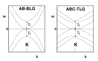
Figure 1: Schematic drawing of the band structure of AB-stacked bilayer graphene (left) and ABC-stacked trilayer graphene (right) in the minimal model for wave vector $\mathbf{k}$ near the valley point $K.$

The 2BM has been used extensively in the literature to study the phase diagram of the C2DEG as well as its transport and optical properties.PhaseDiagram ; Lambert2013 ; Rondeau2013 ; Barlas2012 ; Macdo2012 The phase diagram, up to now, has been mostly studied as a function of magnetic field and bias $\Delta_{B},$ and at integer filling of the eight or twelve sub-Landau levels in $M=0$. To appreciate these studies or add corrections such as screening where Landau levels $\left|M\right|>0$ are important, or to study the phase diagram in higher Landau levels, one must know the limits of validity of the 2BM. In the perturbation theory outlined in Appendix A, the 2BM for BLG is estimated to be valid for low-energy excitations $\left|E\right|<<\gamma_{1},$ and for magnetic field such that $\gamma_{1}v_{3}/v_{0}^{2}<\hslash/\ell<\gamma_{1}/2v_{0}$ where $v_{i}=\frac{\sqrt{3}}{2}\frac{a_{0}}{\hslash}\left|\gamma_{i}\right|$ and $\gamma_{3}$ is the so-called warping term. A similar condition also applies in TLG.

In this work, we use a numerical approach to obtain a more precise evaluation of the range of validity of the 2BM. A numerical computation of the Landau level energies and eigenstates allows the inclusion of all important hopping terms in the tight-binding model and thus give a more realistic description of the levels that goes beyond that of the minimal modelGuinea2006 ; Yuan2011 ; Pereira2007 when values of the hopping parameters typical of those found in the literatureCastro2010 ; Zhang2010 are used. We compare the Landau level energies and eigenstates in the full tight-binding model (in the continuum approximation) with the predictions of the 2BM in a wide range of magnetic field and bias. In our study, we pay particular attention to the eight (BLG) or twelve (TLG) states in $M=0$ since it is for these levels that the 2BM is best suited.

This paper is organized in the following way. In Sec. II, we introduce the AB-BLG and ABC-TLG systems as well as the tight-binding models that give the Landau level spectrum of the full tight-binding model (4BM or 6BM) and of the effective 2BM. In Sec. III, we discuss the effect of the different hopping parameters $\gamma_{i}$ on the Landau level spectrum, we compare the full and effective models for different values of the warping terms $\gamma_{2},\gamma_{3},$ bias and magnetic field and discuss the range of validity of the effective model by comparing the eigenenergies and eigenstates in the two models. We conclude in Sec. IV. In Appendix A, we review the derivation of the 2BM.

II AB-BILAYER AND ABC-TRILAYER GRAPHENE

The crystal structures of the AB-BLG and ABC-TLG (hereafter abbreviated as BLG and TLG) are given in Fig. 2(a),(b) and their tight-binding parameters are defined in Fig. 2(b),(c). (Note that a different labelling is used for equivalent sites in the two structures.) The crystal structure in each graphene layer is a honeycomb lattice that can be described as a triangular Bravais lattice with a basis of two carbon atoms $A_{n}$ and $B_{n}$ where $n$ is the layer index. The triangular lattice constant $a_{0}=2.\,\allowbreak 46$ Å $=\sqrt{3}c,$ where $c=1.42$ Å is the separation between two adjacent carbon atoms. The unit cell of the BLG (TLG) structure has four (six) carbon atoms. The distance between two adjacent graphene layers is $d\approx 3.4$ Å. The Brillouin zone of the reciprocal lattice is hexagonal and has two nonequivalent valley points $\mathbf{K}_{\xi}=\left(\frac{2\pi}{a_{0}}\right)\left(\xi\frac{2}{3},0\right)$ where $\xi=\pm$ is the valley index.

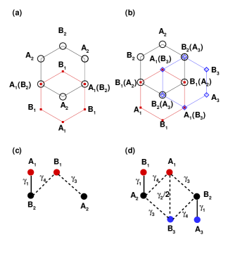
Figure 2: (Color online) Crystal structure of the (a) Bernal-stacked bilayer graphene and (b) ABC-stacked trilayer graphene. Definition of the hopping parameters for the: (c) bilayer and (d) trilayer systems.

The band structure of BLG or TLG is obtained with a tight-binding HamiltonianMcCann2006 ; Koshino2009 ; Zhang2010 ; Partoens2006 . The hopping parameters common to both structures are: $\gamma_{0}$ the nearest-neighbor (NN) hopping in each layer, $\gamma_{1}$ the interlayer hopping between carbon atoms that are immediately above one another, $\gamma_{3}$ the interlayer NN hopping term between carbon atoms of different sublattices, and $\gamma_{4}$ the interlayer next NN hopping term between carbons atoms in the same sublattice. In the trilayer, the extra hopping term $\gamma_{2}$ connects the two low-energy sites $A_{1}$ and $B_{3}$ in Fig. 2.

In the continuum approximation, the tight-binding Hamiltonian is expanded to linear order in the wave vector $\mathbf{p}_{\pm}=\mathbf{k}-\mathbf{K}_{\pm}$. The effect of a magnetic field $\mathbf{B=}B\widehat{\mathbf{z}}$ perpendicular to the graphene layers is then taken into account by making the Peierls substitution $\mathbf{p}\rightarrow\mathbf{P}=\mathbf{p}+e\mathbf{A}/\hslash c$ (with $e>0$ for an electron), where $\mathbf{A}$ is the vector potential of the magnetic field.

II.1 AB bilayer graphene

In a magnetic field, the tight-binding Hamiltonian in the basis $\left\{A_{1},B_{1},A_{2},B_{2}\right\}$ for valley $K_{-}$ and $\left\{B_{2},A_{2},B_{1},A_{1}\right\}$ for valley $K_{+}$ is given by

$$H_{\xi}=\left(\begin{array}[]{cccc}\delta_{0}-\xi\frac{\Delta_{B}}{2}&\xi\alpha_{0}a&\xi\alpha_{4}a^{{\dagger}}&-\gamma_{1}\\ \xi\alpha_{0}a^{{\dagger}}&-\xi\frac{\Delta_{B}}{2}&\xi\alpha_{3}a&\xi\alpha_{4}a^{{\dagger}}\\ \xi\alpha_{4}a&\xi\alpha_{3}a^{{\dagger}}&\xi\frac{\Delta_{B}}{2}&\xi\alpha_{0}a\\ -\gamma_{1}&\xi\alpha_{4}a&\xi\alpha_{0}a^{{\dagger}}&\delta_{0}+\xi\frac{\Delta_{B}}{2}\end{array}\right),$$ (1)

where

$$\alpha_{i}=\sqrt{\frac{3}{2}}\frac{a_{0}}{\ell}\gamma_{i},$$ (2)

and $\delta_{0}$ represents the difference in the crystal field between sites $A_{1},B_{2}$ and $A_{2},B_{1}.$ The energy $\Delta_{B}$ is the potential difference (or bias) between the two outermost layers due to an external electric field perpendicular to the layers.

The Hamiltonian $H_{\xi}^{\left(0\right)}$ obtained from $H_{\xi}$ by setting $\alpha_{3}=0$ has eigenvalues $E_{N,j}^{\left(0\right)}$ and eigenspinors of the form

$$\Psi_{N,j,X}^{\left(0\right)}\left(\mathbf{r}\right)=\left(\begin{array}[]{c}c_{N,j,1}h_{N-1,X}\left(\mathbf{r}\right)\\ c_{N,j,2}h_{N,X}\left(\mathbf{r}\right)\\ c_{N,j,3}h_{N-2,X}\left(\mathbf{r}\right)\\ c_{N,j,4}h_{N-1,X}\left(\mathbf{r}\right)\end{array}\right),$$ (3)

where $N\geq 0.$ In the Landau gauge $\mathbf{A}=\left(0,Bx,0\right)$, the functions $h_{n,X}\left(\mathbf{r}\right)$ are given by

$$h_{n,X}\left(\mathbf{r}\right)=\frac{1}{\sqrt{L_{y}}}e^{-iXy/\ell^{2}}\varphi_{n}\left(x-X\right),$$ (4)

where $L_{y}$ is the length of the 2DEG in the $y$ direction, $X$ the guiding-center index, $\ell=\sqrt{\hslash c/eB}$ the magnetic length and $\varphi_{n}\left(x\right)$ are the wave functions of the one-dimensional harmonic oscillator with quantum number $n=0,1,2,...$ The ladder operators are defined such that $a\varphi_{n}\left(x\right)=-i\sqrt{n}\varphi_{n-1}\left(x\right)$ and $a^{{\dagger}}\varphi_{n}\left(x\right)=i\sqrt{n+1}\varphi_{n+1}\left(x\right).$

The eigenvalues and coefficients $c_{N,j,k}$ for the eigenvectors are found by diagonalizing the matrix

$$F_{1}=\left(\begin{array}[]{cccc}\delta_{0}-\xi\frac{\Delta_{B}}{2}&-\xi i\alpha_{0}g_{N}&\xi\alpha_{4}ig_{N-1}&-\gamma_{1}\\ i\xi\alpha_{0}g_{N}&-\xi\frac{\Delta_{B}}{2}&0&\xi\alpha_{4}ig_{N}\\ -i\xi\alpha_{4}g_{N-1}&0&\xi\frac{\Delta_{B}}{2}&-\xi i\alpha_{0}g_{N-1}\\ -\gamma_{1}&-\xi i\alpha_{4}g_{N}&\xi i\alpha_{0}g_{N-1}&\delta_{0}+\xi\frac{\Delta_{B}}{2}\end{array}\right).$$ (5)

In $\Psi_{N,j,X}^{\left(0\right)}\left(\mathbf{r}\right)$ and in the above equation (and similar ones below), we define $h_{N,X}\left(\mathbf{r}\right)=0$ if $N<0$ and

$$g_{N}=\Theta\left(N\right)\sqrt{N},$$ (6)

where $\Theta\left(N\right)$ is the step function.  For example, with $N=0,$ there can be only one eigenspinor ($j=1$) which is given by (we drop hereafter the $\mathbf{r}$-dependency to simplify the notation) $\Psi_{0,1,X}^{\left(0\right)}=\left(0,h_{0,X},0,0\right)$ and its energy is precisely $E_{0,1}^{\left(0\right)}=-\xi\frac{\Delta_{B}}{2}$ . For $N=1,$ there are three eigenstates ($j=1,2,3$) and four for $N>1$ (i.e. $j=1,2,...,4).$ The energies $E_{N,j}^{\left(0\right)}$ and coefficients $c_{N,j,k}$ ($k=1,2,3,4)$ are independent of the guiding-center index $X$ so that the Landau levels have the usual degeneracy $N_{\varphi}=S/2\pi\ell^{2}$ where $S$ is the 2DEG area. (These energies and coefficients also depend on the valley index $\xi$ but we do not indicate this in order to simplify the notation.) In the basis $\left\{\Psi_{N,j,X}^{\left(0\right)}\right\}$ of the eigenspinors of $H_{\xi}^{\left(0\right)},$ the matrix elements

$$\left\langle\Psi_{N,j,X}^{\left(0\right)}\left|H_{\xi}^{\left(0\right)}\right|\Psi_{M,k,X^{\prime}}^{\left(0\right)}\right\rangle=\delta_{X,X^{\prime}}\delta_{N,M}\delta_{j,k}E_{N,j}^{\left(0\right)}.$$ (7)

The effect of the warping term $\alpha_{3}$ is obtained by diagonalizing the full matrix $H_{\xi}=H_{\xi}^{\left(0\right)}+W_{\xi}$ where $W_{\xi}$ contains only the $\alpha_{3}$ terms and has the matrix elements

$$\left\langle\Psi_{N,j,X}^{\left(0\right)}\left|W_{\xi}\right|\Psi_{M,k,X^{\prime}}^{\left(0\right)}\right\rangle$$

$$= -i\xi\alpha_{3}\sqrt{M-2}c_{N,j,2}^{\ast}c_{M,k,3}\delta_{N,M-3}\delta_{X,X^{\prime}}$$

$$+i\xi\alpha_{3}\sqrt{M+1}c_{N,j,3}^{\ast}c_{M,k,2}\delta_{N,M+3}\delta_{X,X^{\prime}}.$$

This perturbation couples the eigenspinors $\Psi_{N,j,X}^{\left(0\right)}$ with the same $X$ and, in view of Eq. (7), the matrix to diagonalize is the same for all $X^{\prime}s.$ We thus drop the $X$ index hereafter. If the highest Landau level kept in the calculation is $N_{\max},$ then the matrix for $H_{\xi}$ to diagonalize has order $4N_{\max}.$

The two-band model for bilayer grapheneMcCann2006 ; McCannRevue2013 can be obtained in a number of ways. We describe one such way in Appendix A. In the basis $\left(B_{1},A_{2}\right)$ for $K_{-}$ and $\left(A_{2},B_{1}\right)$ for $K_{+},$ the effective two-band Hamiltonian is

$$\widetilde{H}_{\mathbf{\xi}}=\left(\begin{array}[]{cc}-\xi\frac{\Delta_{B}}{2}+\zeta_{+}a^{{\dagger}}a&\frac{\alpha_{0}^{2}}{\gamma_{1}}\left(a^{{\dagger}}\right)^{2}\\ \frac{\alpha_{0}^{2}}{\gamma_{1}}a^{2}&\xi\frac{\Delta_{B}}{2}+\zeta_{-}aa^{{\dagger}}\end{array}\right),$$ (9)

where

$$\beta = \frac{\alpha_{0}}{\gamma_{1}},$$ (10)

$$\zeta = 2\beta\alpha_{4}+\beta^{2}\delta_{0},$$ (11)

$$\zeta_{\pm} = \zeta\pm\xi\beta^{2}\Delta_{B},$$ (12)

The 2BM, as we define it here, does not include the warping term $\gamma_{3}.$

The eigenspinors of the 2BM are of the form

$$\widetilde{\Psi}_{N,j}=\left(\begin{array}[]{c}c_{N,j,1}h_{N}\\ c_{N,j,2}h_{N-2}\end{array}\right).$$ (13)

The $N=0$ eigenvector (with $j=1$) is $\widetilde{\Psi}_{0,1}=\left(h_{0},0\right)$ and has energy

$$\widetilde{E}_{0,1}^{\left(0\right)}=-\xi\frac{\Delta_{B}}{2}.$$ (14)

For $N=1,$ the eigenvector (with $j=1$) is $\widetilde{\Psi}_{1,1}=\left(h_{1},0\right)$ with energy

$$\widetilde{E}_{1,1}^{\left(0\right)}=-\xi\frac{\Delta_{B}}{2}+\zeta_{+}.$$ (15)

The Landau levels are obtained by diagonalizing the matrix

$$F_{2}=\left(\begin{array}[]{cc}-\xi\frac{\Delta_{B}}{2}+\zeta_{+}g_{N}^{2}&-\frac{\alpha_{0}^{2}}{\gamma_{1}}g_{N}g_{N-1}\\ -\frac{\alpha_{0}^{2}}{\gamma_{1}}g_{N}g_{N-1}&\xi\frac{\Delta_{B}}{2}+\zeta_{-}g_{N-1}^{2}\end{array}\right).$$ (16)

For $N>1$, the index $j=1,2.$

In the minimal model ($\gamma_{0},\gamma_{1}\neq 0$ only), the Landau level spectrum is given by $E_{M}=$sgn$\left(M\right)\frac{\alpha_{0}^{2}}{\gamma_{1}}\sqrt{\left|M\right|\left(\left|M\right|+1\right)}.$ The $N=0$ and $N=1$ states are degenerate and are part of the Landau level $M=0.$ Below we refer to these states as the states $n=0$ and $n=1$ of $M=0$ where $n$ is the orbital index in the eigenspinor $\left(h_{n},0\right).$ The index $N\geq 0$ that we use to classify the Landau levels in our numerical analysis is different from the Landau level $M.$ For $N\geq 2$ in Eq. (16), the relation is $M=\pm\left(N-1\right).$

II.2 ABC-stacked trilayer graphene

We repeat the above procedure to get the Landau levels of the ABC-TLG. The tight-binding Hamiltonian in the basis $\left(A_{1},B_{3},B_{1},A_{2},B_{2},A_{3}\right)$ for $K_{+}$ and $\left(B_{3},A_{1},A_{3},B_{2},A_{2},B_{1}\right)$ for $K_{-}$ is

$$H_{\xi}=\left(\begin{array}[]{cccccc}\xi\frac{\Delta_{B}}{2}+\delta_{0}&\frac{\gamma_{2}}{2}&\xi\alpha_{0}a&\xi\alpha_{4}a&\xi\alpha_{3}a^{{\dagger}}&0\\ \frac{\gamma_{2}}{2}&-\xi\frac{\Delta_{B}}{2}+\delta_{0}&0&\xi\alpha_{3}a&\xi\alpha_{4}a^{{\dagger}}&\xi\alpha_{0}a^{{\dagger}}\\ \xi\alpha_{0}a^{{\dagger}}&0&\xi\frac{\Delta_{B}}{2}&\gamma_{1}&\xi\alpha_{4}a&0\\ \xi\alpha_{4}a^{{\dagger}}&\xi\alpha_{3}a^{{\dagger}}&\gamma_{1}&0&\xi\alpha_{0}a&\xi\alpha_{4}a\\ \xi\alpha_{3}a&\xi\alpha_{4}a&\xi\alpha_{4}a^{{\dagger}}&\xi\alpha_{0}a^{{\dagger}}&0&\gamma_{1}\\ 0&\xi\alpha_{0}a&0&\xi\alpha_{4}a^{{\dagger}}&\gamma_{1}&-\xi\frac{\Delta_{B}}{2}\end{array}\right),$$ (17)

where the energy $\delta_{0}$ represents the difference in the crystal field between sites $A_{1},B_{3}$ and sites $A_{2},A_{3},B_{1},B_{2}.$ (In Eq. (17), it is assumed that the middle layer is at zero potential and that $\Delta_{B}$ is the potential difference between the two outermost layers.)

We define $H_{\xi}^{\left(0\right)}$ as the Hamiltonian with $\gamma_{3}$ and $\gamma_{2}$ set to zero. Its eigenspinors are of the form

$$\Psi_{N,j}^{\left(0\right)}=\left(\begin{array}[]{c}c_{N,j,1}h_{N-3}\\ c_{N,j,2}h_{N}\\ c_{N,j,3}h_{N-2}\\ c_{N,j,4}h_{N-2}\\ c_{N,j,5}h_{N-1}\\ c_{N,j,6}h_{N-1}\end{array}\right).$$ (18)

There is only one solution for $N=0$ (with the energy $E_{0,1}^{\left(0\right)}=-\xi\frac{\Delta_{B}}{2}+\delta_{0}$ and $j=1$), three solutions for $N=1$ $(j=1,2,3),$ five solutions for $N=2$ (i.e. $j=1,2,...,5$) and six for $N>2$ (i.e. $j=1,2,...,6$). The matrix to diagonalize is

$$F_{3}=\left(\begin{array}[]{cccccc}\xi\frac{\Delta_{B}}{2}+\delta_{0}&0&-i\xi\alpha_{0}g_{N-2}&-i\xi\alpha_{4}g_{N-2}&0&0\\ 0&-\xi\frac{\Delta_{B}}{2}+\delta_{0}&0&0&i\xi\alpha_{4}g_{N}&i\xi\alpha_{0}g_{N}\\ i\xi\alpha_{0}g_{N-2}&0&\xi\frac{\Delta_{B}}{2}&\gamma_{1}&-i\xi\alpha_{4}g_{N-1}&0\\ i\xi\alpha_{4}g_{N-2}&0&\gamma_{1}&0&-i\xi\alpha_{0}g_{N-1}&-i\xi\alpha_{4}g_{N-1}\\ 0&-i\xi\alpha_{4}g_{N}&i\xi\alpha_{4}g_{N-1}&i\xi\alpha_{0}g_{N-1}&0&\gamma_{1}\\ 0&-i\xi\alpha_{0}g_{N}&0&i\xi\alpha_{4}g_{N-1}&\gamma_{1}&-\xi\frac{\Delta_{B}}{2}\end{array}\right).$$ (19)

The Landau levels are obtained by diagonalizing the full matrix $H_{\mathbf{\xi}}=H_{\mathbf{\xi}}^{\left(0\right)}+W_{\mathbf{\xi}}$ where $W_{\mathbf{\xi}}$ contains only the elements of $H_{\mathbf{\xi}}$ with $\gamma_{2}$ and $\alpha_{3}.$ The matrix elements of $W_{\mathbf{\xi}}$ in the basis $\left\{\Psi_{N,j}^{\left(0\right)}\right\}$ of the eigenvectors of $H_{\xi}^{\left(0\right)}$ are given by

$$\left\langle\Psi_{N,j}^{\left(0\right)}\left|W_{\xi}\right|\Psi_{M,k}^{\left(0\right)}\right\rangle$$

$$= \frac{\gamma_{2}}{2}\left(\delta_{N-3,M}c_{N,j,1}^{\ast}c_{M,k,2}+\delta_{N+3,M}c_{N,j,2}^{\ast}c_{M,k,1}\right)$$

$$-\delta_{N+3,M}i\xi\alpha_{3}\left(c_{N,j,2}^{\ast}c_{M,k,4}g_{M-2}+c_{N,j,5}^{\ast}c_{M,k,1}g_{M-3}\right)$$

$$+\delta_{N-3,M}i\xi\alpha_{3}\left(c_{N,j,4}^{\ast}c_{M,k,2}g_{M+1}+c_{N,j,1}^{\ast}c_{M,k,5}g_{M}\right).$$

If the highest Landau level kept in the calculation is $N_{\max},$ the matrix to diagonalize has order $6\left(N_{\max}-2\right)+9.$

For the two-band model, the basis is $\left(A_{1},B_{3}\right)$ for $H_{K_{+}}$ and $\left(B_{3},A_{1}\right)$ for $H_{K_{-}}$ and the Hamiltonian is given by

$$\widetilde{H}_{\xi}=\left(\begin{array}[]{cc}\delta_{0}+\xi\frac{\Delta_{B}}{2}-\widetilde{\zeta}_{+}aa^{{\dagger}}&\xi\frac{\alpha_{0}^{3}}{\gamma_{1}^{2}}a^{3}\\ \xi\frac{\alpha_{0}^{3}}{\gamma_{1}^{2}}\left(a^{{\dagger}}\right)^{3}&\delta_{0}-\xi\frac{\Delta_{B}}{2}-\widetilde{\zeta}_{-}a^{{\dagger}}a\end{array}\right).$$ (21)

It does not include the $\gamma_{2}$ and $\gamma_{3}$ couplings. In this equation,

$$\widetilde{\zeta}_{\pm}=\zeta\pm\frac{1}{2}\xi\beta^{2}\Delta_{B}.$$ (22)

The eigenvectors of $\widetilde{H}_{\xi}$ have the form

$$\widetilde{\Psi}_{N,j}=\left(\begin{array}[]{c}c_{N,j,1}h_{N-3}\\ c_{N,j,2}h_{N}\end{array}\right).$$ (23)

There is one solution only (i.e. $j=1$) for $N=0,1,2$ which are $\widetilde{\Psi}_{0,1}=\left(0,h_{0}\right),\widetilde{\Psi}_{1,1}=\left(0,h_{1}\right),\widetilde{\Psi}_{2,1}=\left(0,h_{2}\right)$ with energy

$$\widetilde{E}_{0,1}=\delta_{0}-\xi\frac{\Delta_{B}}{2},$$ (24)

$$\widetilde{E}_{1,1} = \left(1-\beta^{2}\right)\delta_{0}$$

$$-\xi\left(1-\beta^{2}\right)\frac{\Delta_{B}}{2}-2\beta\alpha_{4},$$

and

$$\widetilde{E}_{2,1} = \left(1-2\beta^{2}\right)\delta_{0}$$

$$-\xi\left(1-2\beta^{2}\right)\frac{\Delta_{B}}{2}-4\beta\alpha_{4}.$$

For $N>2,$ there are two solutions and the index $j=1,2.$

As in BLG, these three solutions are degenerate in the minimal model and they belong to Landau level $M=0.$ Below, we refer to them as the orbital states $n=0,1,2$ of $M=0.$ The Landau level quantization in the minimal model is $E_{M}=$ sgn$\left(M\right)\frac{\alpha_{0}^{3}}{\gamma_{1}^{2}}\sqrt{\left(\left|M\right|+2\right)\left(\left|M\right|+1\right)\left|M\right|}$ while, for $\widetilde{H}_{\xi},$ the Landau level spectrum is obtained by diagonalizing the matrix

$$F_{4}=\left(\begin{array}[]{cc}\delta_{0}+\xi\frac{\Delta_{B}}{2}-\widetilde{\zeta}_{+}g_{N-2}^{2}&i\xi\frac{\alpha_{0}^{3}}{\gamma_{1}^{2}}g_{N}g_{N-1}g_{N-2}\\ -i\xi\frac{\alpha_{0}^{3}}{\gamma_{1}^{2}}g_{N}g_{N-1}g_{N-2}&\delta_{0}-\xi\frac{\Delta_{B}}{2}-\widetilde{\zeta}_{-}g_{N}^{2}\end{array}\right).$$ (27)

With $N\geq 3$ in $F_{4},$ we obtain the energy of the Landau levels $M=\pm\left(N-2\right).$

III NUMERICAL RESULTS

Each of the four or six bands in the band structure shown in Fig. 1 leads to a set of Landau levels. Since we are interested in comparing the full four-band (4BM) or six-band (6BM) models with the 2BM, we need to consider only the Landau levels originating from the two low-energy bands. In addition, the Landau level spectrum has the symmetry $E_{N,j}\left(\xi,\Delta_{B}\right)=E_{N,j}\left(-\xi,-\Delta_{B}\right)$ and so we can further restrict our analysis to the spectrum in one valley. We choose the valley $K_{+}$. For the numerical calculations, we use the parameters: $\gamma_{0}=3.16$ eV, $\gamma_{1}=0.502$ eV, $\gamma_{2}=-0.0171$ eV, $\gamma_{3}=-0.377$ eV, $\gamma_{4}=-0.099$ eV, $\delta_{0}=-0.0014$ eV for TLGZhang2010 and $\gamma_{0}=3.12$ eV, $\gamma_{1}=0.39$ eV, $\gamma_{3}=0.29$ eV, $\gamma_{4}=0.12$ eV, $\delta_{0}=0.0156$ eV for BLGCastro2010 ; Nilsson2008 . These parameters are not all precisely known and can be affected by correlation effects and substrate.Gruneis2008 However, small changes from these values should not affect significantly our conclusions concerning the validity of the 2BM.

III.1 Analytical criteria for the validity of the two-band model

For the 2BM to be a valid approximation, the energy $\left|E\right|$ of the Landau levels must be much smaller than the inter-layer hopping energy $\gamma_{1}$ i.e. smaller than the energy of the higher-energy bands. In the minimal model $E\sim\alpha_{0}^{2}/\gamma_{1}$ for BLG and $E\sim\alpha_{0}^{3}/\gamma_{1}^{2}$ for TLG. If we require that $E<\gamma_{1}/4$, then the condition of validity of the 2BMMcCann2006 is $\hslash/\ell<\gamma_{1}/2v_{0}$ (BLG) and $\hslash/\ell<\gamma_{1}/2^{4/3}v_{0}$ (TLG), where $v_{i}=\frac{\sqrt{3}}{2}\frac{a_{0}}{\hslash}\left|\gamma_{i}\right|.$ For our choice of parameters, this condition implies that $B\lesssim 56$ T for BLG and TLG.

The warping terms $\gamma_{2},\gamma_{3}$ can also be included in the 2BM. For BLG, this means adding to the Hamiltonian in Eq. (9) the term

$$\widetilde{H}_{w,\mathbf{\xi}}=\xi\alpha_{3}\left(\begin{array}[]{cc}0&a\\ a^{{\dagger}}&0\end{array}\right)$$ (28)

and computing the eigenvalues numerically. For TLG, the warping term $\gamma_{3}$ contributesKoshino2009 a term of order $2\alpha_{0}\alpha_{3}/\gamma_{1}.$ If we require the warping term energy to be smaller than the typical Landau level energy, then we need $\hslash/\ell>\gamma_{1}v_{3}/v_{0}^{2}$ for BLG and $\hslash/\ell>2\gamma_{1}v_{3}/v_{0}^{2}$ for TLG. With our choice of parameters, this implies $B\gtrsim 2$ T for BLG and $B\gtrsim$ $21$ T for TLG. In TLG, we arrive at approximately the same magnetic field if we require that $\left|\gamma_{2}\right|/2<\alpha_{0}^{3}/\gamma_{1}^{2},$ where $\left|\gamma_{2}\right|/2$ is the typical energy contribution for the hopping term $\gamma_{2}.$

III.2 Effect of the hopping terms $\gamma_{2},\gamma_{3}$

We start our analysis by looking at the effect of the hopping terms $\gamma_{2}$ and $\gamma_{3}$ that couple the eigenspinors $\Psi_{N,j}^{\left(0\right)}$ together. For an AB-BLG, the effect of the warping term $\gamma_{3}$ is discussed in Ref. McCann2006, but within the 2BM. Fig. 3 of that paper shows how the $\gamma_{3}$ term couples the Landau levels in the 2BM when $\gamma_{4},\delta_{0}=0$. For small $\alpha=\gamma_{3}/\gamma_{0},$ the Landau level spectrum is almost independent of $\gamma_{3}$ while, at larger value of $\alpha,$ groups of four consecutive levels become degenerate, each group being separated from the next by two nondegenerate Landau levels. In BLG, the value of $\gamma_{3}/\gamma_{0}\approx 0.09$ is such that $\gamma_{3}$ has very little effect on the spectrum if the magnetic field is large enough i.e. for $B\gtrsim 1$ T. This is in good agreement with the analytical result given previously.

Figure 3 of our paper shows our numerical results for the effect of $\gamma_{3}$ on the Landau level spectrum but calculated in the 4BM. We reach the same conclusion as in Ref. McCann2006, i.e. the warping term affects the spectrum only at very small magnetic field. For $B\gtrsim 1$ T, the effect of $\gamma_{3}$ is already very small. The dispersion of the levels with $\gamma_{3}/\gamma_{0},$ however, is qualitatively different than that of the 2BM. In the 4BM, groups of three instead of four consecutive levels become degenerate. We can reproduce this behavior with the 2BM if we include $\gamma_{3}$ and $\gamma_{4}$ in the two-band Hamiltonian i.e. if we add to Eq. (9) the warping term of Eq. (28) and solve using the procedure described in Sec. II. The dispersion of the resulting levels is shown by the blue squares in Fig. 3. Note that, in this figure, the magnetic field is small and so the 4BM and 2BM (with warping) are in good agreement.

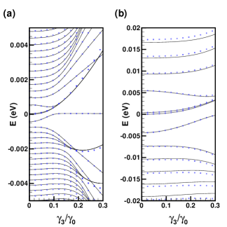
Figure 3: Landau level spectrum as a function of the ratio $\gamma_{3}/\gamma_{0}$ at zero bias in the four-band (lines) and two-band (blue squares) model of BLG for (a) $B=0.1$ T and (b) $B=1.0$ T. The two-band model considered in this figure includes the warping term $\gamma_{3}.$

In the 6BM of TLG, the $\gamma_{2}$ term leads to Landau levels that are degenerate by groups of three at small magnetic field (see also Fig. 9 (d) below). We thus set this term to zero in order to study the effect of the warping term $\gamma_{3}$. At field $B=0.1$ T, Fig. 4 (a) shows that the warping term leads to an important modification of the Landau level spectrum for $\left|\gamma_{3}/\gamma_{0}\right|=0.12$ corresponding to the estimated value of the ratio of $\gamma_{3}$ and $\gamma_{0}$ in TLG. At the larger magnetic field $B=10$ T, Fig. 4 (b) shows that the effect of $\gamma_{3}$ is still noticeable. It becomes negligible at a magnetic field $B\approx 20$ T (this can also be seen in Fig. 5 (d) below).

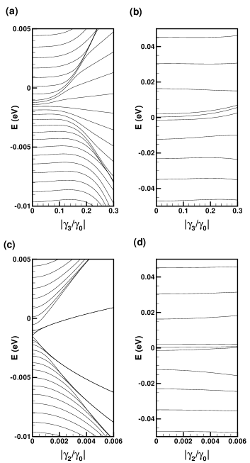
Figure 4: Landau level spectrum in TLG at zero bias in the six-band model as a function of the ratio $\left|\gamma_{3}/\gamma_{0}\right|$ with $\gamma_{2}=0$ for (a) $B=1$ T and (b) $B=10$ T and as a function of the ratio $\left|\gamma_{2}/\gamma_{0}\right|$ with $\gamma_{3}=0$ for (c) $B=1$ T and (d) $B=10$ T.

Figure 4 (c),(d) shows the same analysis but with $\gamma_{3}=0$ and varying $\left|\gamma_{2}/\gamma_{0}\right|.$ Again, the spectrum is strongly influenced by $\gamma_{2}$ at low field. It becomes independent of $\gamma_{2}$ at a magnetic field of the order of $B=20$ T for our choice of hopping parameters i.e. $\left|\gamma_{2}/\gamma_{0}\right|=0.0054.$ This value is again in agreement with the analytical result given above. For TLG, it is necessary to go to much larger magnetic fields than in BLG to avoid the Landau level degeneracy caused by $\gamma_{2}$ and $\gamma_{3}.$

III.3 Dispersion with magnetic field

In this section, we compute the dispersion of the first few Landau levels with magnetic field at zero bias. The result is shown in Fig. 5(a),(b) for BLG and Fig. 5(c),(d) for TLG. The black lines are for the full (4BM or 6BM) Hamiltonian while the blue squares are the 2BM dispersions. Figure 5 (b) and (d) shows an enlarged portion of the low-energy sector that contains the sub-levels in $M=0$ i.e. $n=0,1$ for BLG and $n=0,1,2$ for TLG.

For BLG, warping term $\gamma_{3}$ in the 4BM leads to a very small upward shift $\sim 10^{-4}$ eV of the $n=0$ level with respect to the 2BM where this level is exactly at zero energy. (This small shift is also visible in Fig. 3 (b).) Otherwise, the 2BM overestimates the Landau level energies at all magnetic fields. The energy difference increases with magnetic field and with Landau level index. For example, at $B=30$ T, the difference in energy between the 4BM and 2BM is $25\%,35\%$ and $51\%$ for $n=1,M=1$ and $M=2$ respectively. For $n=1$, the linear dependence of the energy predicted by the 2BM is lost at $B\approx 10$ T in the 4BM. For the higher Landau levels, the accuracy of the 2BM is poor excepted at small magnetic fields.

For TLG, the effects of $\gamma_{2},\gamma_{3}$ are important for $B\lesssim 20$ T and, in this range of magnetic field, there is a great disparity between the full and 2BM even for the $n=0,1,2$ levels in $M=0$ whose energy is otherwise well estimated by the 2BM at higher magnetic field. The linear dependence of the energy with magnetic field given by the 2BM for $n=0,1,2$ is only present for $B\gtrsim 10$ T in TLG. The energy difference between the 6BM and 2BM at $B=30$ T is $0.1\%,16\%,18\%,39\%$ and $59\%$ for $n=0,1,2$ and $M=1,2$ respectively. As in BLG, the energy difference between the full and 2BM increases with Landau level index $\left|M\right|$ and with magnetic field.

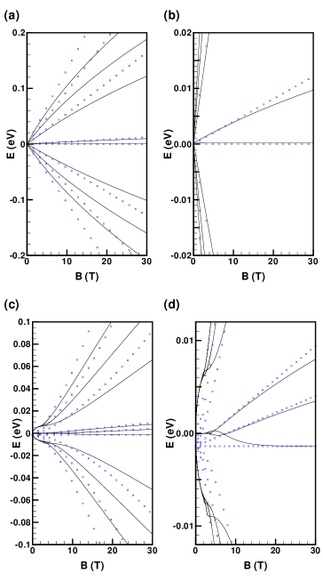
Figure 5: (Color online) Behavior of the Landau levels with magnetic field at zero bias for valley $K_{+}$ for the four-band model (lines) and two-band model without $\gamma_{2}$ and $\gamma_{3}$ (blue squares). (a) bilayer graphene; (b) low-energy sector showing the $M=0$ levels of (a); (c) trilayer graphene; (d) low-energy sector showing the $M=0$ levels of (c).

We showed above that, in BLG and TLG, the 2BM is expected to be valid for magnetic fields $B<56$ T. In the numerical analysis, important quantitative differences between the 4BM and 2BM appear at magnetic fields much smaller than this value. In fact, the energy of the Landau level $M=1$ at $B=30$ T is already near the expected limit of validity of the 2BM which is $E\approx\gamma_{1}/4$.

For magnetic fields $B>1$ T, the Landau level energies in our calculation converge for $N_{\max}=100.$ When the magnetic field is decreased, $N_{\max}$ must be increased, however. In Fig. 5, we have set $N_{\max}=900.$ The $\sqrt{B}$ behavior of the Landau level at small magnetic field in TLG is clearly visible in Fig. 5(c) and (d). As expected, the levels with small energy converge more rapidly with $N_{\max}$ than those with high energy.

III.4 Dispersion with bias $\Delta_{B}$

Figure 6 shows the dependence of the first Landau levels with bias for BLG for the 4BM (black lines) and the 2BM (blue squares) at magnetic fields $B=10$ T and $B=30$ T. The comparison between the two models is quite good in BLG for $M=0$ (and even for $M=\pm 1$ at $B=10$ T). For $\left|M\right|>1,$ however, the 2BM is quantitatively wrong and does not even give the correct qualitative dispersion with bias. This is not surprising since the Landau level energy for $\left|M\right|=2$ is above $\gamma_{1}/4.$

To estimate the range of validity of the 2BM for the $M=0$ levels, we consider the range of bias where the energies in the two models are close and where the $M=0$ levels have lower energy than the $M=\pm 1$ levels. For $B=10$ T and BLG, this range is roughly given by $\Delta_{B}\in\left[-0.1,0.1\right]$ eV while for $B=30$ T, it is extended to $\Delta_{B}\in\left[-0.22,0.18\right].$ Note that a bias $\Delta_{B}=0.1$ eV corresponds to an electric field of $E=150$ mV/nm which is in the experimentally accessible range.Weitz2010

Because $\gamma_{4}\neq 0$ in our calculation, the two levels in $M=0$ in BLG meet at a finite negative (positive) bias $\Delta_{B}^{\ast}$ in valley $K_{+}$($K_{-}$) instead of at $\Delta_{B}^{\ast}=0$. For $\Delta_{B}<\Delta_{B}^{\ast}$ (valley $K_{+}$) in Fig. 6, the order of the $n=0,1$ levels is reversed i.e. $E_{n=1}<E_{n=0}$. From Eqs. (14,15), $\Delta_{B}^{\ast}=-\delta_{0}-2\gamma_{1}\gamma_{4}/\gamma_{0}=-0.046$ eV for the values of the hopping parameters considered in this paper. This change in the relative position of the $n=0,1$ energy levels leads to interesting physics when Coulomb interaction is introduced because the Coulomb exchange energy is more negative in level $n=0$ than in level $n=1.$ The kinetic energy can thus compete with the exchange energy to create broken-symmetry states with orbital coherence when $E_{n=1}\leq E_{n=0}.$Lambert2013 This state is characterized by a finite density of electric dipoles all pointing in the same direction in space.Shizuya2009

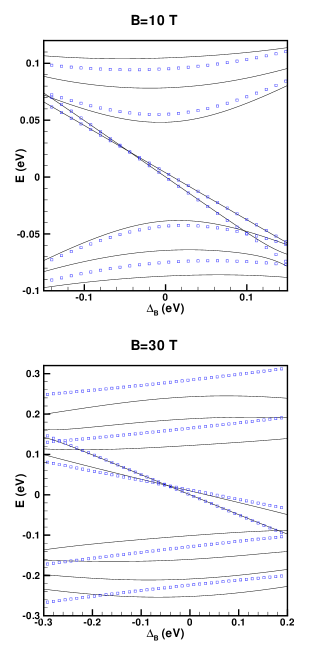
Figure 6: (Color online) Dispersion of the first few Landau levels with bias for the four-band model (lines) and two-band model without $\gamma_{3}$ (blue squares) at magnetic field $B=10$ T and $B=30$ T for bilayer graphene.

Figure 7 shows the dependence of the first Landau levels with bias in TLG for the 6BM (black lines) and the 2BM (blue squares) at magnetic fields $B=10$ T and $B=30$ T. The $\gamma_{2}$ and $\gamma_{3}$ terms are important at $B=10$ T and the range of validity of the 2BM for the $M=0$ Landau levels is dramatically reduced to $\Delta_{B}\in\left[-0.032,0.005\right]$ eV for $B=10$ T. For $B=30$ T, this range is extended to $\Delta_{B}\in\left[-0.14,0.10\right]$ eV. In TLG, as in BLG, the range of validity increases with magnetic field. In TLG, however, there is a region around the crossing point of the $n=0,1,2$ levels predicted in valley $K_{+}$ by the 2BM i.e. $\Delta_{B}^{\ast}=2\left(\delta_{0}+2\gamma_{1}\gamma_{4}/\gamma_{0}\right)=-0.06$ eV, (i.e. in the range $\Delta_{B}\approx\left[-0.07,-0.05\right]$) where the 6BM gives three crossings of the $n=0,1,2$ levels (see Fig. 8). The energy ordering of the levels with increasing bias is $n=\left(2,1,0\right)\rightarrow\left(2,0,1\right)\rightarrow\left(0,2,1\right)\rightarrow\left(0,1,2\right).$ The multiple crossings disappear if $\gamma_{4}$ is set to zero in which case there is a single crossing at the value predicted by the 2BM. This multiple crossing behavior is not captured by the 2BM. When Coulomb interaction is added to the picture, these multiple crossings should lead to a variety of broken-symmetry states with orbital coherence and so to a rich phase diagram for the C2DEG in this range of bias.

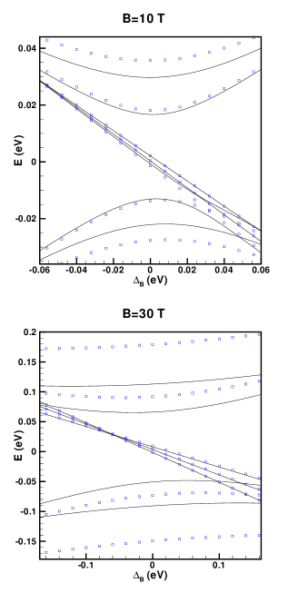
Figure 7: (Color online) Dispersion of the first few Landau levels with bias for the six-band model (lines) and two-band model without $\gamma_{2},\gamma_{3}$ (blue squares) at magnetic field $B=10$ T and $B=30$ T for trilayer graphene.

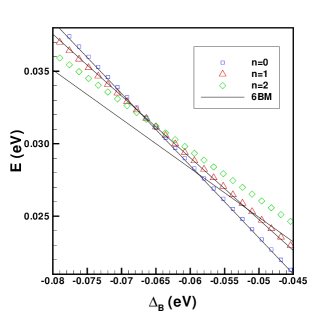
Figure 8: (Color online) Dispersion of the three Landau levels $n=0,1,2$ in $M=0$ with bias in trilayer graphene at $B=30$ T showing the multiple crossings in the 6BM (black lines). The symbols are for the 2BM without $\gamma_{2},\gamma_{3}.$

III.5 Effect of the hopping terms on the Landau level spectrum

It is interesting to see the change in the Landau level spectrum as the different hopping terms are successively turned on at zero bias in TLG. This is shown in Fig. 9. At the top of each figure, we indicate what hopping terms are non zero. In the minimal model with $\gamma_{0},\gamma_{1}\neq 0$ only showing that levels $n=0,1,2$ in $M=0$ are degenerate. With $\delta_{0}\neq 0$ the spectrum is very slightly shifted downwards since $\delta_{0}<0$ and the degeneracy of the $n=0,1,2$ levels is lifted. The energy of levels $n=1,2$ now depends linearly on the magnetic field (see Eqs. (24-II.2)). With $\gamma_{4}\neq 0$ the downward shift is maintained and the slope of the $n=0,1,2$ levels with magnetic field is increased. With the addition of $\gamma_{2},$ the spectrum is shifted upwards and crossings occur between the $n=0,1,2$ levels at small magnetic field (not visible in this figure but noticeable in Fig. 5 (d)). The dispersion of the higher energy levels with magnetic field changes from a $\sqrt{B}$ behavior at small $B$ to a $B^{3/2}$ behavior at larger magnetic field. This occurs at energies $\delta_{0}-\gamma_{2}/2=0.007$ eV and $\delta_{0}+\gamma_{2}/2=-0.01$ eV. Groups of three levels become degenerate at very small magnetic field. (See also Refs. Koshino2009, ; Morimoto2012, where a similar band spectrum is presented.) Finally, the addition of $\gamma_{3}$ (see Fig. 5 (d)) leads to a small downward shift of the spectrum in Fig. 9 (d) but does not introduce other significant qualitative changes.

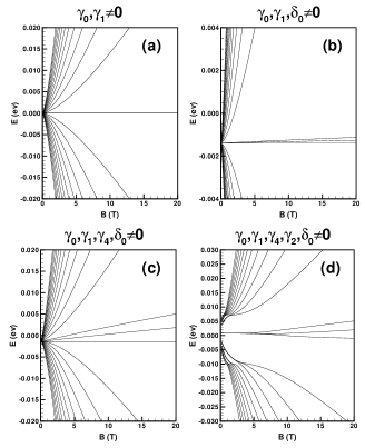
Figure 9: Dispersion of the Landau levels with magnetic field at zero bias in the six-band model of trilayer graphene: (a) minimal model; (b) with the addition of $\delta_{0};$(c) with the further addition of $\delta_{0}$ and $\gamma_{4}$ and (d) with the further addition of $\delta_{0},\gamma_{4}$ and $\gamma_{2}.$

III.6 Eigenstates in the two- and six-band model

In BLG, the eigenspinors given by Eqs. (3) are coupled together by the hopping term $\gamma_{3}.$ In order to diagonalize the full Hamiltonian $H_{\xi},$ we used in Sec. II the basis $\left\{\Psi_{N=0,1}^{\left(0\right)},\Psi_{N=1,1}^{\left(0\right)},\Psi_{N=1,2}^{\left(0\right)},\Psi_{N=1,3}^{\left(0\right)},\Psi_{N>1,k}^{\left(0\right)},...\right\}$ (with $k=1,...,4$) of the eigenstates of $H_{\xi}^{\left(0\right)}$ where the spinors $\Psi_{N,k}^{\left(0\right)}$ for a given $N$ are ordered is ascending order of their energy $E_{N,k}^{\left(0\right)}.$ The eigenstates $\Phi^{\left(j\right)}$ of $H_{\xi}$ can be written as linear combinations of the basis spinors i.e.

$$\Phi^{\left(j\right)}=\sum_{J\left(N,k\right)}b_{J\left(N,k\right)}^{\left(j\right)}\Psi_{N,k}^{\left(0\right)},$$ (29)

where the coefficients $b_{k}^{\left(j\right)}$ are obtained by numerically diagonalizing the full matrix $H_{\xi}.$ If $n_{vec}$ eigenspinors are kept, then $j,J=1,...,n_{vec}$ with the super-index $J\left(N,k\right)$ defined by

$$J\left(0,1\right) = 1,$$ (30)

$$J\left(1,1\right) = 2,$$ (31)

$$J\left(1,2\right) = 3,$$ (32)

$$J\left(1,3\right) = 4,$$ (33)

$$J\left(N>1,k\right) = 4\left(N-1\right)+k.$$ (34)

In this section, we are interested in comparing the eigenstates of Landau level $M=0$ in the 4BM or 6BM and 2BM. We start by considering BLG and later generalize the approach to TLG.

For BLG, the two eigenstates are the $n=0,1$ states that disperse linearly with bias in Fig. 6. In the 4BM, we denote these eigenstates by $\Phi^{\left(j_{0}\right)}$ and $\Phi^{\left(j_{1}\right)}$. In the absence of coupling due to the warping term,

$$\Phi^{\left(j_{0}\right)} = \Psi_{N=0,1}^{\left(0\right)}\Longrightarrow b_{1}^{\left(j_{0}\right)}=1,$$ (35)

$$\Phi^{\left(j_{1}\right)} = \Psi_{N=1,2}^{\left(0\right)}\Longrightarrow b_{3}^{\left(j_{1}\right)}=1,$$ (36)

and so the importance of the coupling can be measured by computing the probabilities

$$P_{0} = \left|b_{1}^{\left(j_{0}\right)}\right|^{2},$$ (37)

$$P_{1} = \left|b_{3}^{\left(j_{1}\right)}\right|^{2}.$$ (38)

The smaller the value of $P_{0},P_{1}$, the more important is the coupling.

In the 2BM, an electron in the $j_{0}$ or $j_{1}$ Landau level is assumed to reside mostly on site $A_{2}$ (for valley $K_{+}$) and to be described by the wave function $h_{0,X}\left(\mathbf{r}\right)$ for $j_{0}$ and $h_{1,X}\left(\mathbf{r}\right)$ for $j_{1}.$ According to Eq. (A) in Appendix A, the occupation of the other sites are of order $2$ in the small quantities defined in this Appendix. In the 4BM, however, the eigenstate is given by the spinor of Eq. (3) and for level $j_{1},$ there may be some electronic amplitude on two other sites of the unit cell i.e. $B_{2}$ and $A_{1}.$ To measure how well the 2BM describes the 4BM eigenstate in levels $j_{0},j_{1},$ we define the probabilities

$$\Lambda_{0} = P_{0}\left|c_{N=0,1,2}\right|^{2},$$ (39)

$$\Lambda_{1} = P_{1}\left|c_{N=1,3,2}\right|^{2}.$$ (40)

(Note that $\left|c_{N=0,1,2}\right|^{2}=1$ so that $P_{0}=\Lambda_{0}.$)

We repeat the above procedure for the TLG system, defining in a similar way the probabilities $P_{n}$ and $\Lambda_{n}$ for $n=0,1,2$. Our numerical results are shown in Fig. 10 for BLG and Fig. 11 for TLG.

Figure 10 shows the probabilities $P_{n}$ and $\Lambda_{n}$ as well as the dispersion of the $n=0,1$ levels with bias in BLG at magnetic field of (a) $10$ T and (b) $30$ T. The range of bias is $\Delta_{B}\in\left[-0.1,0.1\right]$ eV for $B=10$ T and $\Delta_{B}\in\left[-0.22,0.18\right]$ eV for $B=30$ T corresponding to the domain of validity for the 2BM established in Sec. III (C). In this figure, $P_{0},P_{1}\gtrsim 0.98$ at both magnetic fields and the warping term has very little effect on the eigenstate. The eigenvectors $\Psi_{N=0,1}^{\left(0\right)}$ and $\Psi_{N=1,2}^{\left(0\right)}$ are only slightly coupled to the other eigenstates of $H_{\xi}^{\left(0\right)}.$ The coupling decreases with increasing magnetic field as noted before. The probability $\Lambda_{0}\approx 0.98$ for $B=10$ T and $\Lambda_{0}\approx 0.99$ for $B=30$ T so that the $n=0$ 2BM eigenvector is a good approximation of the 4BM eigenvector in this case. For $n=1,\Lambda_{1}\approx 0.90$ for $B=10$ T and $\Lambda_{1}\approx 0.78$ for $B=30$ T so that the 2BM eigenvector for $n=1$ is not as good an approximation as the 2BM eigenvector for $n=0.$

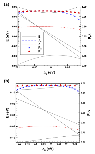
Figure 10: (Color online) Low-energy eigenstates of the four-band model and the probabilities $P$ and $\Lambda$ as a function of bias for the $M=0;n=0,1$ levels of bilayer graphene at (a) $B=10$ T and (b) $B=30$ T.

Figure 11 shows the probabilities $P_{n}$ and $\Lambda_{n}$ as well as the dispersion of the $n=0,1,2$ levels with bias in TLG at magnetic field of (a) $10$ T and (b) $30$ T. The domain of validity of the 2BM is $\Delta_{B}\in\left[-0.032,0.005\right]$ eV for $B=10$ T and $\Delta_{B}\in\left[-0.14,0.10\right]$ eV for $B=30.$ In this figure, $P_{0},P_{1},P_{2}\gtrsim 0.96$ at $B=30$ T and so both magnetic fields and the warping term has very little effect in this case. At the lower $B=10$ T field, however, the coupling is noticeable for level $n=0$. This is what causes the $n=0$ Landau level to increase in energy for $B\lesssim 10$ T in Fig. 5 (d). As in BLG, the probabilities $\Lambda_{n}$ decrease with magnetic field and so the amplitude of the wave function on sites other than those prescribed by the 2BM are not negligible for $B=30$ T and $n=1,2.$ In the region of the multiple crossings (in the range $\Delta_{B}\in\left[-0.07,-0.05\right]$), the levels $n=0,1,2$ cross each other but do not become coupled. In consequence, each level keeps its orbital character in the sense that the amplitude of the wave function for level $n$ is maximal in the orbital $h_{n}\left(\mathbf{r}\right).$

The fact that the electronic amplitude is not small on the high-energy sites at large magnetic field means that the physical quantities such as electric current and electromagnetic absorption are not correctly estimated in the 2BM.

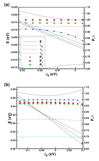
Figure 11: (Color online) Low-energy eigenstates of the six-band model and the probabilities $P$ and $\Lambda$ as a function of bias for the $M=0;n=0,1,2$ levels of trilayer graphene at (a) $B=10$ T and (b) $B=30$ T.

IV CONCLUSION

The two-band model is a useful approximation to study the transport and optical properties of the chiral two-dimensional electron gas in bilayer and trilayer graphene but it is important to know its range of applicability. In this paper, we have compared the Landau level spectrum of the full 6BM (TLG) and 4BM (BLG) as a function of magnetic field and bias with the predictions of the 2BM. We can summarize our main conclusions as follows: (a) the 2BM is generally a better approximation in BLG than in TLG; (b) it describes satisfactorily the $M=0$ Landau levels but differences with the 4BM or 6BM spectrum increase rapidly with increasing Landau level index $\left|M\right|$ and magnetic field; (c) the coupling terms $\gamma_{3}$ in BLG and $\gamma_{2},\gamma_{3}$ in TLG have little effect on the Landau level spectrum at magnetic field $B\gtrsim 1$ T in BLG and $B\gtrsim 10$ T in TLG; (d) at fixed magnetic field and varying bias, the range of validity of the 2BM increases with magnetic field but is much smaller in TLG than in BLG; (e) for TLG, the multiple crossings between the $M=0$ levels that occur within a small range of bias in the 6BM are not captured by the 2BM and so the 2BM may miss some interesting ground states of the C2DEG when Coulomb interaction is added to the non-interacting Hamiltonian; (f) the amplitude of the electronic wave function on sites other than those prescribed by the 2BM for the $M=0$ eigenstates increases with magnetic field and is not negligible at large field; (g) the 2BM consistently overestimates the Landau level energies.

Appendix A DERIVATION OF THE TWO-BAND MODEL

Combining the approaches found in Refs. McCannRevue2013, ; Zhang2010, , we introduce the two-band model in the following way. The eigenvalue equation to be solved can be written in the form

$$\left(\begin{array}[]{cc}H_{1,1}&H_{1,2}\\ H_{2,1}&H_{2,2}\end{array}\right)\left(\begin{array}[]{c}\left|\Psi_{1}\right\rangle\\ \left|\Psi_{2}\right\rangle\end{array}\right)=\varepsilon\left(\begin{array}[]{c}\left|\Psi_{1}\right\rangle\\ \left|\Psi_{2}\right\rangle\end{array}\right),$$ (41)

with the normalization condition

$$\left\langle\Psi_{1}|\Psi_{1}\right\rangle+\left\langle\Psi_{2}|\Psi_{2}\right\rangle=1,$$ (42)

where $H_{1,1}$ is the Hamiltonian for the low-energy sector, $H_{2,2}$ the Hamiltonian of the high-energy sector and $H_{1,2},H_{2,1}$ the coupling terms. In BLG, $H_{i,j}$ are $2\times 2$ matrices and $\Psi_{1},\Psi_{2}$ have $2$ elements. In TLG, $H_{1,1}$ is a $2\times 2$ matrix, $H_{2,2}$ a $4\times 4$ matrix and $H_{1,2},H_{2,1}$ are $2\times 4$ and $4\times 2$ matrices respectively and $\Psi_{1}$ has $2$ elements and $\Psi_{2}$ has $4.$ We want to derive an equation for the low-energy part $\Psi_{1}$ of the eigenspinor.

The eigenvalue equation is rewritten as

$$\left(H_{11}-\varepsilon I\right)\left|\Psi_{1}\right\rangle+H_{12}\left|\Psi_{2}\right\rangle = 0,$$ (43)

$$H_{21}\left|\Psi_{1}\right\rangle+\left(H_{22}-\varepsilon I\right)\left|\Psi_{2}\right\rangle = 0.$$ (44)

where $I$ is the unit matrix. Solving for $|\Psi_{2}\rangle$ gives

$$\left|\Psi_{2}\right\rangle=-\left(H_{22}-\varepsilon I\right)^{-1}H_{21}\left|\Psi_{1}\right\rangle$$ (45)

so that

$$\left[\left(H_{11}-\varepsilon I\right)-H_{12}\left(H_{22}-\varepsilon I\right)^{-1}H_{21}\right]|\Psi_{1}\rangle=0.$$ (46)

This is an exact equation.

Now, $H_{22}$ can be diagonalized by the transformation

$$H_{22}=UD_{22}U^{-1}$$ (47)

where $D_{22}$ is the diagonal matrix containing the eigenvalues of $H_{22}$. It follows that

$$\left(H_{22}-\varepsilon I\right)^{-1} = \left(U\left(D_{22}-\varepsilon I\right)U^{-1}\right)^{-1}$$

$$= U\left(D_{22}-\varepsilon I\right)^{-1}U^{-1}.$$

For the low energy excitations, all eigenvalues of $D_{22}>>\varepsilon$ so that

$$\frac{1}{d_{22}-\varepsilon}\approx\frac{1}{d_{22}}\left(1+\frac{\varepsilon}{d_{22}}\right).$$ (49)

Hence,

$$\left(D_{22}-\varepsilon I\right)^{-1}\approx D_{22}^{-1}\left(I+\varepsilon D_{22}^{-1}\right),$$ (50)

and so

$$\left(H_{22}-\varepsilon I\right)^{-1}\approx H_{22}^{-1}\left(I+\varepsilon H_{22}^{-1}\right)$$ (51)

to first order in $\varepsilon.$

The Schrödinger equation now becomes

$$H_{eff}\left|\Psi_{1}\right\rangle=\varepsilon\left|\Psi_{1}\right\rangle,$$ (52)

where

$$H_{eff}=\left(I+H_{12}H_{22}^{-2}H_{21}\right)^{-1}\left(H_{11}-H_{12}H_{22}^{-1}H_{21}\right).$$ (53)

We have also,

$$\left|\Psi_{2}\right\rangle = -\left(H_{22}-\varepsilon I\right)^{-1}H_{21}\left|\Psi_{1}\right\rangle$$

$$\approx -H_{22}^{-1}\left(I+\varepsilon H_{22}^{-1}\right)H_{21}\left|\Psi_{1}\right\rangle.$$

In order to satisfy the normalization condition of the original model, we define

$$S=I+H_{12}H_{22}^{-2}H_{21}$$ (55)

and make the transformation

$$\left|\widetilde{\Psi}_{1}\right\rangle=S^{1/2}\left|\Psi_{1}\right\rangle.$$ (56)

The new eigenvalue equation is

$$\widetilde{H}_{eff}\left|\widetilde{\Psi}_{1}\right\rangle=\varepsilon\left|\widetilde{\Psi}_{1}\right\rangle$$ (57)

with

$$\widetilde{H}_{eff} = S^{1/2}H_{eff}S^{-1/2}$$

$$= S^{-1/2}\left(H_{11}-H_{12}H_{22}^{-1}H_{21}\right)S^{-1/2}.$$

Note that using Eq. (A), we can further approximate

$$\left|\Psi_{2}\right\rangle\approx-H_{22}^{-1}H_{21}\left|\Psi_{1}\right\rangle,$$ (59)

so that it is easy to show that

$$\left\langle\widetilde{\Psi}_{1}|\widetilde{\Psi}_{1}\right\rangle\approx\left\langle\Psi_{1}|\Psi_{1}\right\rangle+\left\langle\Psi_{2}|\Psi_{2}\right\rangle=1.$$ (60)

The Hamiltonians $H_{eff}$ and $\widetilde{H}_{eff}$ have the same eigenvalues but $\widetilde{H}_{eff}$ is Hermitian while $H_{eff}$ is not necessarily Hermitian.

The intralayer hopping $\gamma_{0},\gamma_{1}\,$are much larger than the small quantities $\left|\varepsilon\right|,\left|\gamma_{2}\right|,\left|\gamma_{3}\right|,\left|\gamma_{4}\right|,\left|\delta_{0}\right|,\left|\Delta_{B}\right|$. Keeping only the terms that are linear in the small quantities and quadratic (BLG) or cubic (TLG) in the operators $a,a^{{\dagger}}$ leads to the Hamiltonian for BLG and TLG given in the text. Within this approximation, $\widetilde{H}_{eff}$ and $H_{eff}$ are identical and the normalization condition reduces to $\left\langle\Psi_{1}|\Psi_{1}\right\rangle=1$ meaning that there is no amplitude of the wave function on the high-energy sites. (From Eq. (A), the probability to be on a high-energy site is quadratic in the small quantities.)

References

• (1) Edward McCann and Vladimir I. Fal’ko, Phys. Rev. Lett. 96, 086805 (2006).
• (2) For a review of the C2DEG, see: Yafis Barlas, Kun Yang, and A. H. MacDonald, Nanotechnology 23, 052001 (2012).
• (3) Hongki Min and A. H. MacDonald, Phys. Rev. B 77, 155416 (2008).
• (4) A. H. Castro Neto, F. Guinea, N. M. R. Peres, K. S. Novoselov and A. K. Geim, Rev. Mod. Phys. 81, 109 (2009).
• (5) D. S. L. Abergel, V. Apalkov, J. Berashevich, K. Ziegler and Tapash Chakraborty, Advances in Physics 59, 261 (2010).
• (6) M. O. Goerbig, Rev. Mod. Phys. 83, 1193 (2011).
• (7) Edward McCann and Mikito Koshino, Rep. Prog. Phys. 76, 056503 (2013).
• (8) J. Lambert and R. Côté, Phys. Rev. B 87, 115415 (2013).
• (9) Yafis Barlas, R. Côté, and Maxime Rondeau, Phys. Rev. Lett. 109, 126804 (2012).
• (10) R. Côté, Maxime Rondeau, Anne-Marie Gagnon, and Yafis Barlas, Phys. Rev. B 86, 125422 (2012).
• (11) Mikito Koshino and Edward McCann, Phys. Rev. B 80, 165409 (2009).
• (12) Fan Zhang, Bhagawan Sahu, Hongki Min, and A. H. MacDonald, Phys. Rev. B 82, 035409 (2010).
• (13) See for example: Rahul Nandkishore and Leonid Levitov, Phys. Scr. T 146, 015011 (2012); E. V. Gorbar, V. P. Gusynin, and V. A. Miransky, Phys. Rev. B 81, 155451 (2010); JETP Lett. 91, 314 (2010) [Pis’ma v ZhETF 91, 334 (2010)]; E. V. Gorbar, V. P. Gusynin, V. A. Miransky, and I. A. Shovkovy, Phys. Rev. B 85, 235460 (2012); E. V. Gorbar, V. P. Gusynin, Junji Jia, and V. A. Miransky, Phys. Rev. B 84, 235449 (2011); E. V. Gorbar, V. P. Gusynin, A. B. Kuzmenko, and S. G. Sharapov, Phys. Rev. B 86, 075414 (2012); K. Shizuya, Phys. Rev. B 79, 165402 (2009); T. Misumi and K. Shizuya, Phys. Rev. B 77, 195423 (2008).
• (14) Fan Zhang, Dagim Tilahun, and A. H. MacDonald, Phys. Rev. B 85, 165139 (2012).
• (15) F. Guinea, A. H. Castro Neto, and N. M. R. Peres, Phys. Rev. B 73, 245426 (2006).
• (16) Shengjun Yuan, Rafael Roldán, and Mikhail I. Katsnelson, Phys. Rev. B 84, 125455 (2011).
• (17) J. Milton Pereira, Jr., F. M. Peeters, and P. Vasilopoulos, Phys. Rev. B 76, 115419 (2007).
• (18) Eduardo V Castro, K. S. Novoselov, S. V. Morozov, N. M. R. Peres, J. M. B. Lopes dos Santos, Johan Nilsson, F. Guinea, A. K. Geim and A. H. Castro Neto, J. PHys.: Condens. Matter 22, 175503 (2010).
• (19) B. Partoens and F. M. Peeters, Phys. Rev. B 74, 075404 (2006).
• (20) Johan Nilsson, A. H. Castro Neto, F. Guinea, and N. M. R. Peres, Phys. Rev. B 78, 045405 (2008).
• (21) A. Grüneis, C. Attaccalite, L. Wirtz, H. Shiozawa, R. Saito, T. Pichler, and A. Rubio, Phys. Rev. B 78, 205425 (2008).
• (22) R. T. Weitz, M. T. Allen, B. E. Feldman, J. Martin, and A. Yacoby, Science 330, 812 (2010); Seyoung Kim, Kayoung Lee, and E. Tutuc, Phys. Rev. Lett. 107, 016803 (2011).
• (23) K. Shizuya, Phys. Rev. B 79, 165402 (2009).
• (24) Takahiro Morimoto, Mikito Koshino, and Hideo Aoki, Phys. Rev. B 86, 155426 (2012).