Digraphs and cycle polynomials for free-by-cyclic groups.

Abstract.

Let $\phi\in\operatorname{Out}(F_{n})$ be a free group outer automorphism that can be represented by an expanding, irreducible train-track map. The automorphism $\phi$ determines a free-by-cyclic group $\Gamma=F_{n}\rtimes_{\phi}\mathbb{Z},$ and a homomorphism $\alpha\in H^{1}(\Gamma;\mathbb{Z})$. By work of Neumann, Bieri-Neumann-Strebel and Dowdall-Kapovich-Leininger, $\alpha$ has an open cone neighborhood $\mathcal{A}$ in $H^{1}(\Gamma;\mathbb{R})$ whose integral points correspond to other fibrations of $\Gamma$ whose associated outer automorphisms are themselves representable by expanding irreducible train-track maps. In this paper, we define an analog of McMullen’s Teichmüller polynomial that computes the dilatations of all outer automorphism in $\mathcal{A}$.

1. Introduction

There is continually growing evidence of a powerful analogy between the mapping class group $\operatorname{Mod}(S)$ of a closed oriented surfaces $S$ of finite type, and the group of outer automorphisms $\operatorname{Out}(F_{n})$ of free groups $F_{n}$. A recent advance in this direction can be found in work of Dowdall-Kapovich-Leininger [DKL13.1] who developed an analog of the fibered face theory of surface homeomorphisms due to Thurston [Thu86] and Fried [Fri82]. In this paper we develop the analogy further by defining a version of McMullen’s Teichmüller polynomial for surface automorphisms defined in [McM00] in the setting of outer automorphisms.

Fibered face theory for free-by-cyclic groups.

A free-by-cyclic group

$$\Gamma=F_{n}\rtimes_{\phi}\mathbb{Z},$$

is a semi-direct product defined by an element $\phi\in\operatorname{Out}(F_{n})$. If $x_{1},\dots,x_{n}$ are generators of $F_{n}$, and $\phi_{\circ}\in\operatorname{Aut}(F_{n})$ is a representative automorphism in the class $\phi$, then $\Gamma$ has a finite presentation

$$\langle x_{1},\dots,x_{n},s\mid sx_{i}s^{-1}=\phi_{\circ}(x_{i})\quad i=1,\dots,n\rangle.$$

There is a distinguished homomorphism $\alpha_{\phi}\colon\thinspace\Gamma\rightarrow\mathbb{Z}$ induced by projection to the second coordinate. That is, $\alpha_{\phi}$ is an element of $H^{1}(\Gamma;\mathbb{Z})$ and $F_{n}$ is the kernel of $\alpha_{\phi}$.

The deformation theory of free-by-cyclic groups started with the work of Neumann [Neu79] and Bieri-Neumann-Strebel [BNS], where they showed there is an open cone in $H^{1}(\Gamma;\mathbb{R})$ containing all primitive integral element in $H^{1}(\Gamma;\mathbb{R})$ that have finitely generated kernels. In [DKL13.1] Dowdall-Kapovich-Leininger showed that this deformation can be understood geometrically in a possibly smaller cone.

More precisely, assume $\phi\in\operatorname{Out}(F_{n})$ is representable by an expanding irreducible train-track map (see [Kap13] [DKL13.1], and Section 4.1 for definitions). The outer automorphism $\phi\in\operatorname{Out}(F_{n})$ may admit many train-track representatives $f$ and every train-track representative can be decomposed into a sequence of folds ${\sf f}$ [Sta83] which is also non-unique. Dowdall, Kapovich and Leininger showed (see [DKL13.1], Theorems A):

Theorem 1.1 (Dowdall-Kapovich-Leininger).

For $\phi\in\operatorname{Out}(F_{n})$ that is representable by an expanding irreducible train-track map and an associated folding sequence ${\sf f}$, there is an open cone neighborhood $\mathcal{A}_{\sf f}$ of $\alpha_{\phi}$ in $\textup{Hom}(\Gamma;\mathbb{R})$, such that, all primitive integral elements $\alpha\in\mathcal{A}$, are associated to a free-by-cyclic decomposition

$$\Gamma=F_{n_{\alpha}}\rtimes_{\phi_{\alpha}}\mathbb{Z}$$

where $\alpha=\alpha_{\phi_{\alpha}}$ and $\phi_{\alpha}\in\operatorname{Out}(F_{n_{\alpha}})$ is also representable by an expanding irreducible train-track map.

We call $\mathcal{A}_{\sf f}$ a DKL-cone associated to $\phi$.

Main Result

Our main theorem is an analog of results in [McM00] in the setting of the outer automorphism groups (see below for more on the motivation behind the result). For a given $\phi$, there are many DKL cones associated to $\phi$ since $A_{\sf f}$ depends on the choice of the train-track representative $f$ and folding sequence ${\sf f}$. We show that there is a more unified picture. Namely, there is a cone $\mathcal{T}_{\phi}$ depending only on $\phi$ that contains every cone $\mathcal{A}_{\sf f}$. The cone $\mathcal{T}_{\phi}$ is the support of a convex, real analytic, homogenous function $L$ of degree $-1$ whose restriction to every cone $\mathcal{A}_{\sf f}$ is the logarithm of dilatation function. Moreover, this function can be computed via specialization of a single polynomial $\Theta$ that also depends only on $\phi$.

Our approach is combinatorial. We associate a labeled digraph to the splitting sequence ${\sf f}$. This gives a combinatorial description of ${\sf f}$ and in turn defines a cycle polynomial $\theta$ and the cone $\mathcal{T}_{\phi}$. We analyze the effect of certain elementary moves on digraphs and show that their associated cycle polynomial and cone remain unchanged under these elementary moves. We show that as we pass to different fibrations of $\Gamma$ corresponding to other integral points of $\mathcal{A}_{\sf f}$, the digraph changes by elementary moves, as do the digraphs associated to different splitting sequences $f$. This establishes the independence of $\theta$ and $\mathcal{T}_{\phi}$ from the choice of splitting sequence ${\sf f}$. The polynomial $\Theta$ is a factor of the cycle polynomial $\theta$ determined by the log dilatation factor and does not depend on the choice of train track map.

We establish some terminology before stating the main theorem more precisely. For $\phi\in\operatorname{Out}(F_{n})$ that is representable by an expanding irreducible train-track map and a nontrivial $\gamma\in F_{n}$, the growth rate of cyclically reduced word-lengths of $\phi^{k}(\gamma)$ is exponential, with a base $\lambda(\phi)>1$ that is independent of $\gamma$. The constant $\lambda(\phi)$ is called the dilatation (or expansion factor) of $\phi$.

Let $G$ be a finitely generated free abelian group of rank $k$, and let

$$\theta=\sum_{g\in G}a_{g}g,\qquad a_{g}\in\mathbb{Z}$$

be an element of the group ring $\mathbb{Z}G$. For $\alpha\in\textup{Hom}(G;\mathbb{Z})$, the specialization of $\theta$ at $\alpha$ is the single variable integer polynomial

$$\theta^{(\alpha)}(x)=\sum_{g\in G}a_{g}x^{\alpha(g)}\in\mathbb{Z}[x].$$

The house of a $\theta^{(\alpha)}(x)$ is given by

$$\left|\theta^{(\alpha)}\right|=\max\Big{\{}|\mu|\ \mathbin{\Big{|}}\mu\in\mathbb{C},\ \theta^{(\alpha)}(\mu)=0\Big{\}}.$$

Theorem A.

Let $\phi\in\operatorname{Out}(F_{n})$ be an outer automorphism that is representable by an expanding irreducible train-track map, $\Gamma=F_{n}\rtimes_{\phi}\mathbb{Z}$ and let $G=\Gamma^{\mbox{ab}}/{\mbox{Torsion}}$. Then there exists an element $\Theta\in\mathbb{Z}G$ (well-defined up to an automorphism of $\mathbb{Z}G$) with the following properties.

1. There is an open cone $\mathcal{T}_{\phi}\subset\textup{Hom}(G;\mathbb{R})$ dual to a vertex of the Newton polygon of $\Theta$ so that, for any expanding irreducible train-track representative $f\colon\thinspace\tau\rightarrow\tau$ and any folding decomposition ${\sf f}$ of $f$, we have

   $$\mathcal{A}_{\sf f}\subset\mathcal{T}_{\phi}.$$

2. For any integral $\alpha\in\mathcal{A}_{\sf f}$, we have

   $$\big{|}\Theta^{(\alpha)}\big{|}=\lambda(\phi_{\alpha}).$$

3. The function

   $$L(\alpha)=\log\big{|}\Theta^{(\alpha)}\big{|},$$

   which is defined on the primitive integral points of $\mathcal{A}_{\sf f}$, extends to a real analytic, convex function on $\mathcal{T}_{\phi}$ that is homogeneous of degree $-1$ and goes to infinity toward the boundary of any affine planar section of $\mathcal{T}_{\phi}$.

4. The element $\Theta$ is minimal with respect to property (2), that is, if $\theta\in\mathbb{Z}G$ satisfies

   $$\big{|}\theta^{(\alpha)}\big{|}=\lambda(\phi_{\alpha})$$

   on the integral elements of some open sub-cone of $\mathcal{T}_{\phi}$ then $\Theta$ divides $\theta$.

Remark B.

In their original paper [DKL13.1] Dowdall, Kapovich, and Leininger also show that $\log(\lambda(\phi_{\alpha}))$ is convex and has degree $-1$ and in the subsequent paper [DKL13.2], using a different approach from ours, they give an independent definition of an element $\Theta_{\textup{\tiny DKL}}\in\mathbb{Z}G$ with the property that $\lambda(\phi_{\alpha})=\big{|}\Theta_{\mbox{\tiny DKL}}^{(\alpha)}\big{|}$ for $\alpha\in A_{\sf f}$. Property (3) of Theorem A implies that $\Theta$ divides $\Theta_{\mbox{\tiny DKL}}$.

Remark C.

Thinking of $G$ as an abelian group generated by $t_{1},\dots,t_{k}$, we can identify the elements of $G$ with monomials in the symbols $t_{1},\dots,t_{k}$, and hence $\mathbb{Z}G$ with Laurent polynomials in $\mathbb{Z}(t_{1},\dots,t_{k})$. Thus, we can associate to $\theta\in\mathbb{Z}G$ a polynomial $\theta(t_{1},\dots,t_{k})\in\mathbb{Z}(t_{1},\dots,t_{k})$. Identifying $\textup{Hom}(G;\mathbb{Z})$ with $\mathbb{Z}^{k}$, each element $\alpha=(a_{1},\dots,a_{k})$ defines a specialization of $\theta=\theta(t_{1},\dots,t_{k})$ by

$$\theta^{(\alpha)}(x)=\theta(x^{a_{1}},\dots,x^{a_{k}}).$$

For ease of notation, we mainly use the group ring notation through most of this paper.

Motivation from pseudo-Anosov mapping classes on surfaces.

Let $S$ be a closed oriented surface of negative finite Euler characteristic. A mapping class $\phi=[\phi_{\circ}]$ is an isotopy class of homeomorphisms

$$\phi_{\circ}\colon\thinspace S\rightarrow S.$$

The mapping torus $X_{(S,\phi)}$ of the pair $(S,\phi)$ is the quotient space

$$X_{(S,\phi)}=S\times[0,1]/{(x,1)\sim(\phi_{\circ}(x),0)}.$$

Its homeomorphism type is independent of the choice of representative $\phi_{\circ}$ for $\phi$. The mapping torus $X_{(S,\phi)}$ has a distinguished fibration $\rho_{\phi}\colon\thinspace X_{(S,\phi)}\rightarrow S^{1}$ defined by projecting $S\times[0,1]$ to its second component and identifying endpoints. Conversely, any fibration $\rho\colon\thinspace X\rightarrow S^{1}$ of a 3-manifold $X$ over a circle can be written as the mapping torus of a unique mapping class $(S,\phi)$, with $\rho=\rho_{\phi}$. The mapping class $(S,\phi)$ is called the monodromy of $\rho$.

Thurston’s fibered face theory [Thu86] gives a parameterization of the fibrations of a $3$–manifold $X$ over the circle with connected fibers by the primitive integer points on a finite union of disjoint convex cones in $H^{1}(X;\mathbb{R})$, called fibered cones. The dilatation of $\phi$ and is denoted by $\lambda(\phi)$. Thurston showed that the mapping torus of any pseudo-Anosov mapping class is hyperbolic, and the monodromy of any fibered hyperbolic 3-manifold is pseudo-Anosov. It follows that the set of all pseudo-Anosov mapping classes partitions into subsets corresponding to integral points on fibered cones of hyperbolic 3-manifolds.

By results of Fried [Fri82] (cf. [M87] [McM00]) the function $\log\lambda(\phi)$ defined on integral points of a fibered cone $\mathcal{T}$ extends to a continuous convex function

$$\mathcal{Y}\colon\thinspace\mathcal{T}\rightarrow\mathbb{R},$$

that is a homogeneous of degree $-1$, and goes to infinity toward the boundary of any affine planar section of $\mathcal{T}$. The Teichmüller polynomial of a fibered cone $\mathcal{T}$ defined in [McM00] is an element $\Theta_{\mbox{\tiny{Teich}}}$ in the group ring $\mathbb{Z}G$ where $G=H_{1}(X;\mathbb{Z})/{\mbox{Torsion}}$. The group ring $\mathbb{Z}G$ can be thought of as a ring of Laurent polynomials in the generators of $G$ considered as a multiplicative group, and in this way, we can think of $\Theta_{\mbox{\tiny{Teich}}}$ as a polynomial. The Teichmüller polynomial $\Theta_{\mbox{\tiny{Teich}}}$ has the property that the dilatation $\lambda(\phi_{\alpha})$ of every mapping class $\phi_{\alpha}$ associated to an integral point $\alpha\in\mathcal{T}$, $\lambda(\phi_{\alpha})$ can be obtained from $\Theta_{\text{\tiny{Teich}}}$ by taking the house of the specialization. Furthermore, the cone $\mathcal{T}$ and the function $\mathcal{Y}$ are determined by $\Theta_{\text{\tiny{Teich}}}$. Our work is a step towards reproducing this picture in the setting of $\operatorname{Out}(F_{n})$.

Organization of paper

In Section 2 we establish some preliminaries about Perron-Frobenius digraphs $D$ with edges labeled by a free abelian group $G$. Each digraph $D$ determines a cycle complex $C_{D}$ and cycle polynomial $\theta_{D}$ in the group ring $\mathbb{Z}G$. Under certain extra conditions, we define a cone $\mathcal{T}$, which we call the McMullen cone, and show that

$$L(\alpha)=\log|\theta_{D}^{(\alpha)}|$$

defined for integral elements of $\mathcal{T}$ extends to a homogeneous function of degree -1 that is real analytic and convex on $\mathcal{T}$ and goes to infinity toward the boundary of affine planar sections of $\mathcal{T}$. Furthermore, we show the existence of a distinguished factor $\Theta_{D}$ of $\theta_{D}$ with the property that

$$|\Theta_{D}^{(\alpha)}|=|\theta_{D}^{(\alpha)}|,$$

and $\Theta_{D}$ is minimal with this property. Our proof uses a key result of McMullen (see [McM00], Appendix A).

In Section 3 we define branched surfaces $(X,\mathfrak{C},\psi)$, where $X$ is $2$-complex with a semiflow $\psi$, and cellular structure $\mathfrak{C}$ satisfying compatibility conditions with respect to $\psi$. To a branched surface we associate a dual digraph $D$ and a $G$-labeled cycle complex $C_{D}$, where $G=H_{1}(X;\mathbb{Z})/{\mbox{torsion}}$, and a cycle function $\theta_{D}\in\mathbb{Z}G$. We show that $\theta_{D}$ is invariant under certain allowable cellular subdivisions and homotopic modifications of $(X,\mathfrak{C},\psi)$.

In Sections 4 and 5 we study the branched surfaces associated to the train-track map $f$ and folding sequence ${\sf f}$ defined in [DKL13.1], called respectively the mapping torus, and folded mapping torus. We use the invariance under allowable cellular subdivisions and modifications established in Section 2 and Section 3 to show that the cycle functions for these branched surfaces are equal. The results of Section 2 applied to the mapping torus for $f$ imply the existence of $\Theta_{\phi}$ and $\mathcal{T}_{\phi}$ in Theorem A. Applying an argument in [DKL13.1], we show that further subdivisions with the folded mapping torus give rise to mapping tori for train-track maps corresponding to $\phi_{\alpha}$, and use this to show that for $\alpha\in\mathcal{A}_{\sf f}$, we have $\lambda(\phi_{\alpha})=|\Theta_{\phi}^{(\alpha)}|$. We further compare the definition of the DKL cone $\mathcal{A}_{\sf f}$ and $\mathcal{T}_{\phi}$ to show inclusion $\mathcal{A}_{\sf f}\subset\mathcal{T}_{\phi}$, and thus complete the proof of Theorem A.

We conclude in Section 6 with an example where $A_{\sf f}$ is a proper subcone of $\mathcal{T}_{\phi}$.

Acknowledgements.

The authors would like to thank J. Birman, S. Dowdall, N. Dunfield, A. Hadari , C. Leininger, C. McMullen, and K. Vogtman for helpful discussions.

2. Digraphs, their cycle complexes and eigenvalues of $G$-matrices

This section contains basic definitions and properties of digraphs, and a key result of McMullen that will be useful in our proof of Theorem A.

2.1. Digraphs, cycle complexes and their cycle polynomials

We recall basic results concerning digraphs (see, for example, [Gan59] and [CR90] for more details).

Definition 2.1.

A digraph $D$ is a finite directed graph with at least two vertices. Given an ordering $v_{1},\dots,v_{m}$ of the vertices of $D$, the adjacency matrix of $D$ is the matrix

$$M_{D}=[a_{i,j}],$$

where $a_{i,j}=m$ if there are $m$ directed edges from $v_{i}$ to $v_{j}$. The characteristic polynomial $P_{D}$ is the characteristic polynomial of $M_{D}$ and the dilatation $\lambda(D)$ of $D$ is the spectral radius of $M_{D}$

$$\lambda(D)=\max\Big{\{}|e|\,\Big{|}\,\mbox{$e$ is an eigenvalue of $M_{D}$}\Big{\}}.$$

Conversely, any square $m\times m$ matrix $M=[a_{i,j}]$ with non-negative integer entries determines a digraph $D$ with $M_{D}=M$. The digraph $D$ has $m$ vertices and $a_{i,j}$ vertices from the $i$th to the $j$th vertex.

Definition 2.2.

For a matrix $M$, let $a_{ij}^{m}$ be the $ij^{\,\text{th}}$ entry of $M^{m}$. A non-negative matrix $M$ with real entries is called expanding if

$$\limsup_{m\to\infty}a_{ij}^{m}=\infty.$$

A digraph $D$ is expanding if its directed adjacency matrix $M_{D}$ is expanding. Note that an expanding digraph is strongly connected.

An eigenvalue of $M$ is simple if its algebraic multiplicity is 1. Note that several simple eigenvalues may have the same norm. The following theorem is well-known (see, for example, [Gan59]).

Theorem 2.3.

Let $M$ be a matrix and $\lambda(M)$ the maximum of the norm of any eigenvalue of $M$. If $M$ is expanding, then it has a simple eigenvalue with norm equal to $\lambda(M)$ and it has an associated eigenvector that is strictly positive. In addition, for every $i$ and $j$, we have

$$\limsup_{m\to\infty}(a_{ij}^{m})^{\frac{1}{m}}=\lambda(M).$$

Definition 2.4.

A simple cycle $\alpha$ on a digraph $D$ is an isotopy class of embeddings of the circle $S^{1}$ to $D$ oriented compatibly with the directed edges of $D$. A cycle is a disjoint union of simple cycles. The cycle complex $C_{D}$ of a digraph $D$ is the collection of cycles on $D$ thought of as a simplicial complex, whose vertices are the simple cycles.

The cycle complex $C_{D}$ has a measure which assigns to each cycle its length in $D$, that is, if $\gamma$ is a cycle on $C_{D}$, then its length $\ell(\gamma)$ is the number of vertices (or equivalently the number of edges) of $D$ on $\gamma$, and, if $\sigma=\{\gamma_{1},\dots,\gamma_{s}\}$, then

$$\ell(\sigma)=\sum_{i=1}^{s}\ell(\gamma_{i}).$$

Let $|\sigma|=s$ be the size of $\sigma$. The cycle polynomial of a digraph $D$ is given by

$$\theta_{D}(x)=1+\sum_{\sigma\in C_{D}}(-1)^{|\sigma|}x^{-\ell(\sigma)}.$$

Theorem 2.5 (Coefficient Theorem for Digraphs [CR90]).

Let $D$ be a digraph with $m$ vertices, and $P_{D}$ the characteristic polynomial of the directed adjacency matrix $M_{D}$ for $D$. Then

$$P_{D}(x)~{}=~{}x^{m}\theta_{D}(x)$$

Proof.

Let $\mbox{M}_{D}=[a_{i,j}]$ be the adjacency matrix for $D$. Then

$$P_{D}(x) = \mbox{det}(xI-\mbox{M}_{D}).$$

Let $S_{{\sf V}}$ be the group of permutations of the vertices ${\sf V}$ of $D$. For $\pi\in S_{V}$, let $\mbox{fix}(\pi)\subseteq{{\sf V}}$ be the set of vertices fixed by $\pi$, and let $\textup{sign}(\pi)$ be -1 if $\pi$ is an odd permutation and $1$ if $\pi$ is even. Then

$$P_{D}(x) = \sum_{\pi\in S_{{\sf V}}}\textup{sign}(\pi)A_{\pi}$$

where

(1) $$A_{\pi} = \prod_{v\notin\mbox{fix}(\pi)}(-a_{v,\pi(v)})\prod_{v\in\mbox{fix}(\pi)}(x-a_{v,v})$$

There is a natural map $\Sigma:C_{D}\to S_{{\sf V}}$ from the cycle complex $C_{D}$ to the permutation group $S_{{\sf V}}$ on the set ${\sf V}$ defined as follows. For each simple cycle $\gamma$ in $D$ passing through the vertices ${\sf V}_{\gamma}\subset{\sf V}$, there is a corresponding cyclic permutation $\Sigma(\gamma)$ of ${\sf V}_{\gamma}$. That is, if ${\sf V}_{\gamma}=\{v_{1},\dots,v_{\ell}\}$ contains more than one vertex and is ordered according to their appearance in the cycle, then then $\Sigma(\gamma)(v_{i})=v_{i+1(\mbox{\small mod}\ell)}$. If ${\sf V}_{\gamma}$ contains one vertex, we say $\gamma$ is a self-edge. For self-edges $\gamma$, $\Sigma(\gamma)$ is the identity permutation. Let $\sigma=\{\gamma_{1},\dots,\gamma_{s}\}$ be a cycle on $D$. Then we define $\Sigma(\sigma)$ to be the product of disjoint cycles

$$\Sigma(\sigma)=\Sigma(\gamma_{1})\circ\cdots\circ\Sigma(\gamma_{\ell}).$$

The polynomial $A_{\pi}$ in Equation (1) can be rewritten in terms of the cycles $\sigma$ of $C_{D}$ with $\Sigma(\sigma)=\pi$. First we rewrite $A_{\pi}$ as

(2) $$A_{\pi}=\sum_{\nu\subset\mbox{fix}(\pi)}x^{|\mbox{fix}(\pi)-\nu|}\prod_{v\notin\mbox{fix}(\pi)}(-a_{v,\pi(v)})\prod_{v\in\nu}(-a_{v,v}).$$

Let $\pi\in S_{{\sf V}}$ be in the image of $\Sigma$. For a cycle $\sigma\in C_{D}$, let $\nu(\sigma)\subset{\sf V}$ be the subset vertices at which $\sigma$ has a self-edge.

For $\nu\subset\mbox{fix}(\pi)$ let

$$P_{\pi,\nu}=\{\sigma\in C_{D}\ |\ \mbox{$\Sigma(\sigma)=\pi$ and $\nu(\sigma)=\nu$}\}.$$

The we claim that the number of elements in $P_{\pi_{\nu}}$ is

(3) $$\prod_{v\notin\mbox{fix}(\pi)}a_{v,\pi(v)}\prod_{v\in\nu}a_{v,v}.$$

Let $\sigma\in C_{D}$ be such that $\Sigma(\sigma)=\pi$. Then for each $v\in{\sf V}{\smallsetminus}\mbox{fix}(\pi)$, there is a choice of $a_{v,\pi(v)}$ edges from $v$ to $\pi(v)$, and for each $v\in\mbox{fix}(\pi)$ $\sigma$ either contains no self-edge, or one of $a_{v,v}$ possible self-edges at $v$. This proves (3).

For each $\sigma\in C_{D}$, we have

$$\ell(\sigma)=m-|\mbox{fix}(\Sigma(\sigma))|+|\nu(\sigma)|.$$

Thus, the summand in (2) associated to $\pi\in S_{{\sf V}}{\smallsetminus}\mbox{id}$, and $\nu\subset\mbox{fix}(\pi)$ is given by

$$x^{|\mbox{fix}(\pi)|-|\nu|}\prod_{v\notin\mbox{fix}(\pi)}(-a_{v,\pi(v)})\prod_{v\in\nu}(-a_{v,v}) = (-1)^{m-|\mbox{fix}(\pi)|+|\nu|}\sum_{\sigma\in P_{\pi,\nu}}x^{m-\ell(\sigma)}$$

$$= \sum_{\sigma\in P_{\pi,\nu}}(-1)^{\ell(\sigma)}x^{m-\ell(\sigma)},$$

and similarly for $\pi=\mbox{id}$ we have

$$A_{\pi} = \prod_{v\in{\sf V}}(x-a_{v,v})$$

$$= x^{m}+\sum_{\sigma\in P_{\pi,\nu}}(-1)^{\ell(\sigma)}x^{m-\ell(\sigma)}.$$

For each $\sigma\in C_{D}$, $\textup{sign}(\Sigma(\sigma))=(-1)^{\ell(\sigma)-|\sigma|}$. Putting this together, we have

$$P_{D}(x) =\sum_{\pi\in S_{\sf V}}\textup{sign}(\pi)A_{\pi}$$

$$=x^{m}+\sum_{\pi\in S_{\sf V}}\sum_{\sigma\in C_{D}\colon\thinspace\ \Sigma(\sigma)=\pi}(-1)^{\ell(\sigma)-|\sigma|}(-1)^{\ell(\sigma)}x^{m-\ell(\sigma)}$$

$$=x^{m}+\sum_{\sigma\in C_{D}}(-1)^{|\sigma|}x^{m-\ell(\sigma)}.\qed$$

2.2. McMullen Cones

Each group ring element partitions $\textup{Hom}(G;\mathbb{R})$ into a union of cones defined below.

Definition 2.6.

(cf. [McM02]) Let $G$ be a finitely generated free abelian group. Given an element $\theta=\sum_{g\in G}a_{g}g\in\mathbb{Z}G$, the support of $\theta$ is the set

$$\mbox{Supp}(\theta)=\{g\in G\ |\ a_{g}\neq 0\}.$$

Let $\theta\in\mathbb{Z}G$ and $g_{0}\in\mbox{Supp}(\theta)$ the McMullen cone of $\theta$ for $g_{0}$ is the set

$$\mathcal{T}_{\theta}(g_{0})=\{\alpha\in\textup{Hom}(G;\mathbb{R})\mid\alpha(g_{0})>\alpha(g)\ \mbox{for all $g\in\mbox{Supp}(\theta){\smallsetminus}\{g_{0}\}$}\}.$$

Remark 2.7.

The elements of $G$ can be identified with a subset of the dual space

$$\widehat{\textup{Hom}(G;\mathbb{R})}=\textup{Hom}(\textup{Hom}(G;\mathbb{R}),\mathbb{R})$$

to $\textup{Hom}(G;\mathbb{R})$. Let $\theta\in\mathbb{Z}G$ be any element. The convex hull of $\mbox{Supp}(\theta)$ in $\widehat{\textup{Hom}(G;\mathbb{R})}$ is called the Newton polyhedron $\mathcal{N}$ of $\theta$. Let $\widehat{\mathcal{N}}$ be the dual of $\mathcal{N}$ in $\textup{Hom}(G;\mathbb{R})$. That is, each top-dimensional face of $\widehat{\mathcal{N}}$ corresponds to a vertex $g\in\mathcal{N}$, and each $\alpha$ in the cone over this face has the property that $\alpha(g)>\alpha(g^{\prime})$ where $g^{\prime}$ is any vertex of $\mathcal{N}$ with $g\neq g^{\prime}$. Thus, the McMullen cones $\mathcal{T}_{\theta}(g_{0})$, for $g_{0}\in\mbox{Supp}(\theta)$ are the cones over the top dimensional faces of the dual to the Newton polyhedron of $\theta$.

2.3. A coefficient theorem for $H$-labeled digraphs

Throughout this section let $H$ be the free abelian group with $k$ generators and let $\mathbb{Z}H$ be its group ring. Let $G=H\times\langle s\rangle$, where $s$ is an extra free variable. Then the Laurent polynomial ring $\mathbb{Z}H(u)$ is canonically isomorphic to $\mathbb{Z}G$, by an isomorphism that sends $s$ to $u$.

We generalize the results of Section 2.1 to the setting of $H$–labeled digraphs.

Definition 2.8.

Let $C$ be a simplicial complex. An $H$–labeling of $C$ is a map

$$h\colon\thinspace C\rightarrow H$$

compatible with the simplicial complex structure of $H$, i.e.,

$$h(\sigma)=\sum_{i=1}^{\ell}h(v_{i})$$

for $\sigma=\{v_{1},\dots,v_{\ell}\}$. An $H$-complex $\mathcal{C}^{H}$ is an abstract simplicial complex together with a $H$-labeling.

Definition 2.9.

The cycle function of an $H$–labeled complex $\mathcal{C}^{H}$ is the element of $\mathbb{Z}H$ defined by

$$\theta_{\mathcal{C}^{H}}=1+\sum_{\sigma\in\mathcal{C}^{H}}(-1)^{|\sigma|}h(\sigma)^{-1}.$$

Definition 2.10.

An $H$-digraph $\mathcal{D}^{H}$ is a digraph $D$, along with a map

$$h\colon\thinspace\mathcal{E}_{D}\to H,$$

where $\mathcal{E}_{D}$ is the set of edge of $D$. The digraph $D$ is the underlying digraph of $\mathcal{D}^{H}$.

An $H$-labeling on a digraph induces an $H$-labeling on its cycle complex. Let $\gamma$ be a simple cycle on $D$. Then up to isotopy, $\gamma$ can be written as

$$\gamma=e_{0}\cdots e_{k-1},$$

for some collection of edge $e_{0},\dots,e_{k-1}$ cyclically joined end to end on $D$. Let

$$h(\gamma)=h(e_{0})+\ldots+h(e_{k-1}),$$

and for $\sigma=\{\gamma_{1},\dots,\gamma_{\ell}\}$, let

$$h(\sigma)=\sum_{i=1}^{\ell}h(\gamma_{i}).$$

Denote the labeled cycle complex by $\mathcal{C}_{\mathcal{D}}^{H}$.The cycle polynomial $\theta_{\mathcal{D}^{H}}$ of $\mathcal{D}^{H}$ is given by

$$\theta_{\mathcal{D}^{H}}(u)=1+\sum_{\sigma\in\mathcal{C}_{\mathcal{D}}^{H}}(-1)^{|\sigma|}h(\sigma)^{-1}u^{-\ell(\sigma)}\in\mathbb{Z}H[u]=\mathbb{Z}G.$$

The cycle polynomial of $\theta_{\mathcal{D}^{H}}(u)$ contains both the information about the associated labeled complex $\mathcal{C}_{\mathcal{D}}^{H}$ and the length functions on cycles on $D$. One observes the following by comparing Definition 2.9 and Definition 2.10.

Lemma 2.11.

The cycle polynomial of the $H$–labeled digraph $\mathcal{D}^{H}$, and the cycle function of the labeled cycle complex $\mathcal{C}_{\mathcal{D}}^{H}$ are related by

$$\theta_{\mathcal{C}_{\mathcal{D}}^{H}}=\theta_{\mathcal{D}^{H}}(1).$$

Definition 2.12.

An element $\theta\in\mathbb{Z}H$ is positive, denoted $\theta>0$, if

$$\theta=\sum_{h\in H}a_{h}h,$$

where $a_{h}\geq 0$ for all $h\in H$, and $a_{h}>0$ for at least one $h\in H$. If $\theta$ is positive or $0$ we say that it is non-negative and write $\theta\geq 0$.

A matrix $M^{H}$ with entries in $\mathbb{Z}H$ is called an $H$–matrix. If all entries are non-negative, we write $M^{H}\geq 0$ and if all entries are positive we write $M^{H}>0$.

Lemma 2.13.

There is a bijective correspondence between $H$–digraphs $\mathcal{D}^{H}$ and non-negative $H$–matrices $M_{\mathcal{D}}^{H}$, so that $M_{\mathcal{D}}^{H}$ is the directed incidence matrix for $\mathcal{D}^{H}$.

Proof.

Given a labeled digraph $\mathcal{D}^{H}$, let $E_{ij}$ be the set of edges from the $i^{\,\text{th}}$ vertex to the $j^{\,\text{th}}$ vertex. We form a matrix $M_{\mathcal{D}}^{H}$ with entries in $\mathbb{Z}H$ by setting

$$a_{ij}=\sum_{e\in E_{ij}}h(e),$$

where $h(e)$ is the $H$-label of the edge $e$.

Conversely, given an $n\times n$ matrix $M^{H}$ with entries in $\mathbb{Z}H$, let $\mathcal{D}^{H}$ be the $H$-digraph with $n$ vertices $v_{1},\dots,v_{n}$ and, for each $i,j$ with $m_{i,j}=\sum_{h\in H}a_{g}g\geq 0$, it has $a_{h}$ directed edges from $v_{i}$ to $v_{j}$ labeled by $h$. The directed incidence matrix $M^{H}_{\mathcal{D}}$ equals $M$ as desired. ∎

The proof of the next theorem is similar to that of the Theorem 2.5 and is left to the reader.

Theorem 2.14 (The Coefficients Theorem for $H$–labeled digraphs).

Let $\mathcal{D}^{H}$ be an $H$–labeled digraph with $m$ vertices, and $P_{\mathcal{D}}(u)\in\mathbb{Z}H[u]$ be the characteristic polynomial of its incidence matrix. Then,

$$P_{\mathcal{D}}(u)=u^{m}\theta_{\mathcal{D}^{H}}(u).$$

Note that $P_{\mathcal{D}}(u)$ is an element of $\mathbb{Z}G$.

2.4. Expanding $H$–matrices

In this section we recall a key theorem of McMullen on leading eigenvalues of specializations of expanding $H$–matrices (see [McM00], Appendix A). Although McMullen’s theorem is stated for Perron-Frobenius matrices, the proof only uses only that the matrix is expanding.

Definition 2.15.

A labeled digraph $\mathcal{D}^{H}$ is called expanding if the underlying digraph $\mathcal{D}$ is expanding. The $H$–matrix $M_{\mathcal{D}}^{H}$ is defined to be expanding if the associated labeled digraph $\mathcal{D}^{H}$ is expanding.

For the rest of this section, we fix an expanding $H$–labeled digraph $\mathcal{D}^{H}$. Consider an element ${\sf t}\in\textup{Hom}(H,\mathbb{R}_{+})$. Define $M_{\mathcal{D}}^{H}({\sf t})$ to be the real valued matrix obtained by applying ${\sf t}$ to the entries of $M_{\mathcal{D}}^{H}$ (where ${\sf t}$ is extended linearly to $\mathbb{Z}H$). Alternatively, identify $H$ with space of monomials in $k$ variables $t_{1},\ldots,t_{k}$. This gives a natural identification of $\textup{Hom}(H,\mathbb{R}_{+})$ with $\mathbb{R}_{+}^{k}$ where the $i^{\,\text{th}}$ coordinate in $\mathbb{R}_{+}^{k}$ is associated to the variable $t_{i}$. Then $M_{\mathcal{D}}^{H}({\sf t})$ is be the matrix obtained by replacing $t_{i}$ with $i^{\,\text{th}}$ coordinate of ${\sf t}\in\mathbb{R}_{+}^{k}=\textup{Hom}(H,\mathbb{R}_{+})$.

Note that, since $\mathcal{D}^{H}$ is expanding, for every ${\sf t}\in\mathbb{R}_{+}^{k}$, the real valued matrix $M_{\mathcal{D}}^{H}({\sf t})$ is also expanding. Define a function

$$E\colon\thinspace\mathbb{R}_{+}^{k}\to\mathbb{R}_{+},\qquad\text{by}\qquad E({\sf t})=\lambda\big{(}M_{\mathcal{D}}^{H}({\sf t})\big{)}.$$

Identifying the ring $\textup{Hom}(H,\mathbb{R})$ with $\mathbb{R}^{k}$, there is a natural map

$$\exp\colon\thinspace\textup{Hom}(H,\mathbb{R})\to\textup{Hom}(H,\mathbb{R}_{+}),$$

where, for ${\sf w}=(w_{1},\ldots,w_{k})\in\mathbb{R}^{k}$,

$$\exp({\sf w})=(e^{w_{1}},\ldots,e^{w}_{k}).$$

Define

$$\delta\colon\thinspace\mathbb{R}^{k}\to\mathbb{R},\qquad\text{by}\quad\delta({\sf w})=\log E(e^{\sf w}).$$

Note that the graph of the function $\delta$ lives in $\mathbb{R}^{k}\times\mathbb{R}$ which can be naturally identified with $\textup{Hom}(G;\mathbb{R})$.

Theorem 2.16 (McMullen [McM00], Theorem A.1).

For an expanding $H$–labeled digraph $\mathcal{D}^{H}$, we have the following.

1. The function $\delta$ is real analytic and convex.

2. The graph of $\delta$ meets every ray through the origin of $\mathbb{R}^{k}\times\mathbb{R}$ at most once.

3. For $Q(u)$ any factor of $P_{\mathcal{D}}(u)$, where $Q(E({\sf t}))=0$ for all ${\sf t}\in\mathbb{R}_{+}^{k}$, and for $d=\deg(Q)$, the set of rays passing through the graph of $\delta$ in $\mathbb{R}^{k}\times\mathbb{R}$ coincides with the McMullen cone $\mathcal{T}_{Q}(u^{d})$.

Definition 2.17.

For any expanding $H$–labeled digraph $\mathcal{D}^{H}$, let $d=\deg(P_{\mathcal{D}})$. We refer to the cone $\mathcal{T}=\mathcal{T}_{P_{\mathcal{D}}}(u^{d})$ as the McMullen cone for the element $P_{\mathcal{D}}\in\mathbb{Z}G$. Alternatively we refer to it as the McMullen cone for the $H$–matrix $M_{\mathcal{D}}^{H}$.

Theorem 2.18 (McMullen [McM00]).

For any expanding $H$–labeled digraph $\mathcal{D}^{H}$ the map

$$L\colon\thinspace\textup{Hom}(G;\mathbb{Z})\rightarrow\mathbb{R}$$

defined by

$$L(\alpha)=\log|P_{\mathcal{D}}^{(\alpha)}|,$$

extends to a homogeneous of degree $-1$, real analytic, convex function on the McMullen cone $\mathcal{T}$ for the element $P_{\mathcal{D}}$. It goes to infinity toward the boundary of affine planar sections of $\mathcal{T}$.

Theorem 2.18 summarizes results taken from [McM00] given in the context of mapping classes on surfaces. For the convenience of the reader, we give a proof here.

Proof.

The function $L$ is real analytic since the house of a polynomial is an algebraic function in its coefficients. Homogeneity of $L(z)$ follows from the following observation: $\rho$ is a root of $Q(x^{{\sf w}},x^{s})$ if and only if $\rho^{1/c}$ is a root of $Q(x^{c{\sf w}},x^{cs})$. Thus

$$L(cz)=\log|Q(x^{c{\sf w}},x^{cs})|=c^{-1}\log|Q(x^{\sf w},x^{s})|=c^{-1}L(z).$$

By homogeneity of $L$, the values of $L$ are determined by the values at any level set, one of which is the graph of $\delta({\sf w})$. To prove convexity of $L$, we show that level sets of $L$ are convex i.e. the line connecting two points on a level set lies above the level set. Let $\Gamma=\{z=({\sf w},s)\mid L(z)=1\}$ and $\Gamma^{\prime}=\{z=({\sf w},s)\mid s=\delta({\sf w})\}$. We show that $\Gamma=\Gamma^{\prime}$. It then follows that, since $\Gamma^{\prime}$ is a graph of a convex function by Theorem 2.16, $\Gamma$ is convex.

We begin by showing that $\Gamma^{\prime}\subset\Gamma$ (cf. [McM00], proof Theorem 5.3). If $\beta=({\sf a},b)\in\Gamma^{\prime}$ then $\delta({\sf a})=b$, hence $Q(e^{\sf a},e^{b})=0$ and $|Q(e^{\sf a},e^{b})|\geq e$. Let $r=L(\beta)=\log|Q(e^{\sf a},e^{b})|$. Since $b=\delta({\sf a})$, by the convexity of the function $\delta$, we have $rb\geq\delta(r{\sf a})$. On the other hand, $Q(e^{r{\sf a}},e^{rb})=0$ hence $e^{rb}$ is an eigenvalue of $M(e^{r{\sf a}})$ so $rb\leq\log E(e^{r{\sf a}})=\delta(r{\sf a})$. We get that $rb=\delta(r{\sf a})$. The points $({\sf a},b),(r{\sf a},rb)$ both lie on the same line through the origin so by Theorem 2.16 part (2), they are equal. Thus $r=1=L(\beta)$, and hence $\beta\in\Gamma$.

To show that $\Gamma\subset\Gamma^{\prime}$ in $\mathcal{T}$, note that every ray in $\mathcal{T}$ initiating from the origin intersects $\Gamma$ because it intersects $\Gamma^{\prime}$ by part (3) of Theorem 2.16. Because $L$ is homogeneous, level sets of $L$ intersect every ray from the origin at most once. Therefore, in $\mathcal{T}$, $\Gamma=\Gamma^{\prime}$ and the latter is the graph of a convex function.

We now show that if $L$ is a homogeneous function of degree -1, and has convex level sets then $L$ is convex (cf. [McM00] Corollary 5.4). This is equivalent to showing that $1/L(z)$ is concave on $\mathcal{T}$. Let $z_{1},z_{2}\in T$ lie on distinct rays through the origin, and let

$$z_{3}=sz_{1}+(1-s)z_{2}.$$

Let $c_{i}$, $i=1,2,3$, be constants so that $z_{i}^{\prime}=c_{i}^{-1}z_{i}$ is in the level set $L(c_{i}^{-1}z_{i})=1$. Let $p$ lie on the line $[z_{1}^{\prime},z_{2}^{\prime}]$ and on the ray through $z_{3}$. Then $p$ has the form

$$p=rz_{1}^{\prime}+(1-r)z_{2}^{\prime}$$

for $0<r<1$. If

$$r=\frac{sc_{1}}{sc_{1}+(1-s)c_{2}}$$

then we have

$$p=\frac{z_{3}}{sc_{1}^{\prime}+(1-s)c_{2}^{\prime}}.$$

Since the level set for $L(z)=1$ is convex, $p$ is equal to or above $z_{3}/c_{3}$, and we have

(4) $$1/(sc_{1}+(1-s)c_{2})\geq 1/c_{3}.$$

Thus

(5) $$1/L(z_{3})=c_{3}\geq sc_{1}+(1-s)c_{2}=s/L(z_{2})+(1-s)/L(z_{3}).$$

Thus $1/L(z)$ is concave, and hence $L(z)$ is convex.

Let $z_{n}$ be a sequence of points on an affine planar section of $\mathcal{T}$ approaching the boundary of $\mathcal{T}$. Let $c_{n}$ be such that $c_{n}^{-1}z_{n}$ is in the level set $L(z)=1$. Then $L(z_{n})=c_{n}^{-1}$ for all $n$. But $z_{n}$ is bounded, while the level set $L(z)=1$ is asymptotic to the boundary of $\mathcal{T}$. Therefore, $1/L(z_{n})$ goes to 0 as $n$ goes to infinity. ∎

Remark 2.19.

If the level set $L(z)=1$ is strictly convex, then $L(z)$ is strictly convex. Indeed, if $L(z)=1$ is strictly convex, then the inequality in (4) is strict, and hence the same holds for (5).

2.5. Distinguished factor of the characteristic polynomial

We define a distinguished factor of the characteristic polynomial of a Perron-Frobenius $G$-matrix.

Proposition 2.20.

Let $P$ be the characteristic polynomial of a Perron-Frobenius $G$-matrix. Then $P$ has a factor $Q$ with the properties:

1. for all integral elements $\alpha$ in the McMullen cone $\mathcal{T}$,

   $$|P^{(\alpha)}|=|Q^{(\alpha)}|,$$

2. minimality: if $Q_{1}\in\mathbb{Z}G[u]$ satisfies $|Q^{(\alpha)}|=|Q_{1}^{(\alpha)}|$ for all $\alpha$ ranging among the integer points of an open subcone of $\mathcal{T}$, then $Q$ divides $Q_{1}$, and

3. if $r$ is the degree of $Q$ the cones $\mathcal{T}_{P}(u^{d})$ and $\mathcal{T}_{Q}(u^{r})$ are equal, where $d$ is the degree of $P$ and $r$ is the degree of $Q$ as elements of $\mathbb{Z}G[u]$.

Definition 2.21.

Given a Perron-Frobenius $G$-matrix $M^{G}$, the polynomial $Q$ is called the distinguished factor of the characteristic polynomial of $M^{G}$.

Lemma 2.22.

Let $F({\sf t})\colon\thinspace\mathbb{R}^{k}\to\mathbb{R}$ be a function, consider the ideal

$$I_{F}=\{\theta\in\mathbb{Z}({\sf t})[u]\mid\theta({\sf t},F({\sf t}))=0\text{ for all }{\sf t}\in\mathbb{R}^{k}\}$$

$I_{F}$ is a principal ideal.

Proof.

Let $\overline{\mathbb{Z}({\sf t})}[u]$ be the ring of polynomials in the variable $u$ over the quotient field of $\mathbb{Z}({\sf t})$. Since $\overline{\mathbb{Z}}({\sf t})[u]$ is a principal ideal domain, $I_{F}$ generates a principal ideal $\overline{I}_{F}$ in $\overline{\mathbb{Z}({\sf t})}[u]$.

Let $\overline{\theta}_{1}$ be a generator of $\overline{I}_{F}$, then $\overline{\theta_{1}}=\frac{\theta_{1}({\sf t},u)}{\sigma({\sf t})}$ with $\theta_{1}\in I_{F}$. Thus $\overline{\theta}_{1}({\sf t},F({\sf t}))=0$ for all ${\sf t}$. If $I_{F}$ is the zero ideal then there is nothing to prove, therefore we suppose it is not. Let $\overline{\theta}_{1}({\sf t},u)=\frac{\nu({\sf t},u)}{\delta({\sf t})},$ where $\nu$ and $\delta$ are relatively prime in $\overline{\mathbb{Z}({\sf t})}[u]$, a unique factorization domain. Since $\theta_{1}({\sf t},F({\sf t}))=0$ for all ${\sf t}$ then $\nu({\sf t},F({\sf t}))=0$ for all ${\sf t}$ and $\nu\in I_{F}$.

Since $I_{F}$ is not the zero ideal then $\overline{I}_{F}$ is not the zero ideal, hence $\bar{\theta}_{1}\neq 0$ which implies that $\nu\neq 0$. Let $\theta\in I_{F}$ be any polynomial. Since $\overline{\theta}_{1}$ divides $\theta$, then $\nu$ divides $\theta\delta({\sf t})$ but since $\nu$ and $\delta$ are relatively prime, $\nu$ divides $\theta$. Therefore, $\nu$ is a generator of $I_{E}$. ∎

Proof of Proposition 2.20.

The proposition follows from Lemma 2.22 by declaring $Q$ to be the generator of $I_{L}$ for $L\colon\thinspace\mathcal{T}\to\mathbb{R}$ defined in Theorem 2.18. ∎

3. Branched surfaces with semiflows

In this section we associate a digraph and an element $\theta_{X,\mathfrak{C},\psi}\in\mathbb{Z}G$ to a branched surface $(X,\mathfrak{C},\psi)$. We show that this element is invariant under certain kinds of subdivisions of $\mathfrak{C}$.

3.1. The cycle polynomial of a branched surface with a semiflow

Definition 3.1.

Given a 2-dimensional CW-complex $X$, a semiflow on $X$ is a continuous map $\psi\colon\thinspace X\times\mathbb{R}_{+}\to X$ satisfying

1. $\psi(\cdot,0)\colon\thinspace X\to X$ is the identity,

2. $\psi(\cdot,t)\colon\thinspace X\to X$ is a homotopy equivalence for every $t\geq 0$, and

3. $\psi(\psi(x,t_{0}),t_{1})=\psi(x,t_{0}+t_{1})$ for all $t_{0},t_{1}\geq 0$.

A cell-decomposition $\mathfrak{C}$ of $X$ is $\psi$-compatible if the following hold.

1. Each $1$–cell is either contained in a flow line (vertical), or transversal to the semiflow at every point (transversal).

2. For every vertex $p\in\mathfrak{C}^{(0)}$, the image of the forward flow of $p$,

   $$\{\psi(p,t)\ |\ t\in\mathbb{R}_{>0}\},$$

   is contained in $\mathfrak{C}^{(1)}$.

A branched surface is a triple $(X,\mathfrak{C},\psi)$, where $X$ is a 2-complex with semi-flow $\psi$ and a $\psi$-compatible cellular structure $\mathfrak{C}$.

Remark 3.2.

We think of branched surfaces as flowing downwards. From this point of view, Property (2) implies that every $2$–cell $c\in\mathfrak{C}^{(2)}$ has a unique top $1$–cell, that is, a $1$–cell $e$ such that each point in $c$ can be realized as the forward orbit of a point on $e$.

Definition 3.3.

Let $e$ be a $1$–cell on a branched surface $(X,\mathfrak{C},\psi)$ that is transverse to the flow at every point. A hinge containing $e$ is an equivalence class of homeomorphisms $\kappa\colon\thinspace[0,1]\times[-1,1]\hookrightarrow X$ so that:

1. the half segment $\Delta=\{(x,0)\mid x\in I\}$ is mapped onto $e$,

2. the image of the interior of the $\Delta$ intersects $\mathfrak{C}^{(1)}$ only in $e$, and

3. the vertical line segments $\{x\}\times[-1,1]$ are mapped into flow lines on $X$.

Two hinges $\kappa_{1},\kappa_{2}$ are equivalent if there is an isotopy rel $\Delta$ between them. The $2$–cell on $(X,\mathfrak{C},\psi)$ containing $\kappa([0,1]\times[0,1])$ is called the initial cell of $\kappa$ and the $2$–cell containing the point $\kappa([0,1]\times[-1,0])$ is called the terminal cell of $\kappa$.

An example of a hinge is illustrated in Figure 1.

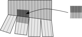
Figure 1. A hinge on a branched surface.

Definition 3.4.

Let $(X,\mathfrak{C},\psi)$ be a branched surface. The dual digraph $D$ of $(X,\mathfrak{C},\psi)$ is the digraph with a vertex for every $2$–cell and an edge for every hinge $\kappa$ from the vertex corresponding to its initial $2$–cell to the vertex corresponding to its terminal $2$–cell. The dual digraph $D$ for $(X,\mathfrak{C},\psi)$ embeds into $X$

$$D\hookrightarrow X$$

so that each vertex is mapped into the interior of the corresponding $2$–cell, and each directed edge is mapped into the union of the two-cells corresponding to its initial and end vertices, and intersects the common boundary of the $2$–cells at a single point. The embedding is well defined up to homotopies of $X$ to itself.

An example of an embedded dual digraph is shown in Figure 2. In this example, there are three edges emanating from $v$ with endpoints at $w_{1},w_{2}$ and $w_{3}$. It is possible that $w_{i}=w_{j}$ for some $i\neq j$, of that $w_{i}=v$ for some $i$. These cases can be visualized using Figure 2, where we identify the corresponding $2$–cells.

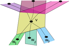
Figure 2. A section of an embedded dual digraph.

Let $G=H_{1}(X;\mathbb{Z})/{\mbox{torsion}}$, thought of as the integer lattice in $H_{1}(X,\mathbb{R})$. The embedding of $D$ in $X$ determines a $G$-labeled cycle complex $\mathcal{C}_{D}^{G}$ where for each $\sigma\in\mathcal{C}_{D}^{G}$ and $g(\sigma)$ is the homology class of the cycle $\sigma$ considered as a 1-cycle on $X$.

Definition 3.5.

Given a branched surface $(X,\mathfrak{C},\psi)$, the cycle function of $(X,\mathfrak{C},\psi)$ is the group ring element

$$\theta_{X,\mathfrak{C},\psi}=1+\sum_{\sigma\in\mathcal{C}_{D}^{G}}(-1)^{|\sigma|}g(\sigma)^{-1}\in\mathbb{Z}G.$$

Then we have

$$\theta_{X,\mathfrak{C},\psi}=\theta_{\mathcal{C}_{D}^{G}}(1)$$

where $\theta_{\mathcal{C}_{D}^{G}}(u)$ is the cycle polynomial of $\mathcal{C}_{D}^{G}$.

3.2. Subdivision

We show that the cycle function of $(X,\mathfrak{C},\psi)$ is not invariant under certain kinds of cellular subdivisions.

Definition 3.6.

Let $p\in\mathfrak{C}^{(1)}$ be a point in the interior of a transversal edge in $\mathfrak{C}^{(1)}$. Let $x_{0}=p$ and inductively define $x_{i}=\psi(x_{i-1},s_{i})$, for $i=1,\dots,r$, so that

$$s_{i}=\min\{s\ |\ \mbox{$\psi(x_{i-1},s)$ has endpoint in $\mathfrak{C}^{(1)}$}\}.$$

The vertical subdivision of $X$ along the forward orbit of $p$ is the cellular subdivision $\mathfrak{C}^{\prime}$ of $\mathfrak{C}$ obtained by adding the edges $\psi(x_{i-1},[0,s_{i}])$, for $i=1,\dots,r$, and subdividing the corresponding $2$–cells. If $x_{r}$ is a vertex in the original skeleton $\mathfrak{C}^{(0)}$ of $X$, then we say the vertical subdivision is allowable.

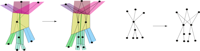
Figure 3. An allowable vertical subdivision, and effect on the directed dual digraph.

Figure 1 illustrates an allowable vertical subdivision with $r=2$.

Proposition 3.7.

Let $(X,\mathfrak{C}^{\prime},\psi)$ be obtained from $(X,\mathfrak{C},\psi)$ by allowable vertical subdivision. Then the cycle function $\theta_{X,\mathfrak{C},\psi}$ and $\theta_{X,\mathfrak{C}^{\prime},\psi}$ are equal.

We establish a few lemmas before proving Proposition 3.7.

Lemma 3.8.

Let $(X,\mathfrak{C}^{\prime},\psi)$ be obtained from $(X,\mathfrak{C},\psi)$ by allowable vertical subdivision. Let $D^{\prime}$ and $D$ be the dual digraphs for $(X,\mathfrak{C}^{\prime},\psi)$ and $(X,\mathfrak{C},\psi)$. There is a quotient map $q\colon\thinspace D^{\prime}\rightarrow D$ that is induced by a continuous map from $X$ to itself that is homotopic to the identity, and in particular the diagram

commutes.

Proof.

Working backwards from the last vertically subdivided cell to the first, each allowable vertical subdivision decomposes into a sequence of allowable vertical subdivisions that involve only one $2$–cell. An illustration is shown in Figure 4.

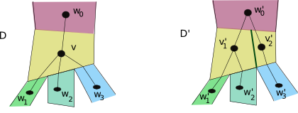
Figure 4. Vertical subdivision of one cell.

Let $v$ be the vertex of $D$ corresponding to the cell $c$ of $X$ that contains the new edge. The digraph $D^{\prime}$ is constructed from $D$ by the following steps:

1. Each vertex $u\neq v$ in $D$ lifts to a well-defined vertex $u^{\prime}$ in $D^{\prime}$. The vertex $v\in D$ lifts to two vertices $v_{1}^{\prime},v_{2}^{\prime}$ in $D^{\prime}$.

2. For each edge $\varepsilon$ of $D$ neither of whose endpoints $u$ and $w$ equal $v$, the quotient map is 1-1 over $\varepsilon$, and hence there is only one possible lift $\epsilon^{\prime}$ from $u^{\prime}$ to $w^{\prime}$.

3. For each edge $\varepsilon$ from $w\neq v$ to $v$ there are two edges $\varepsilon^{\prime}_{1},\varepsilon^{\prime}_{2}$ where $\varepsilon^{\prime}_{i}$ begins at $w^{\prime}$ and ends at $v_{i}^{\prime}$.

4. For each outgoing edge $\varepsilon$ from $v$ to $w$ (where $v$ and $w$ are possibly equal), there is a representative $\kappa$ of the hinge corresponding to $\varepsilon$ that is contained in the union of two $2$–cells in the $\mathfrak{C}^{\prime}$. This determines a unique edge $\varepsilon^{\prime}$ on $D^{\prime}$ that lifts $\varepsilon$.

There is a continuous map homotopic to the identity from $X$ to itself that restricts to the identity on every cell other than $c$ or $c_{w}$, where $c_{w}$ corresponds to a vertex $w$ with an edge from $w$ to $v$ in $D$. On $c\cup c_{w}$ the map merges the edges $\varepsilon^{\prime}_{1},\varepsilon^{\prime}_{2}$ so that their endpoints $v_{i}^{\prime}$ merge to the one vertex $v$. ∎

Lemma 3.9.

The quotient map $q:D\rightarrow D^{\prime}$ induces an inclusion

$$q^{*}:C_{D}\hookrightarrow C_{D^{\prime}},$$

which preserves lengths, sizes, and labels, so that for $\sigma\in C_{D}$, $q(q^{*}(\sigma))=\sigma$.

Proof.

Again we may assume that the subdivision involves a vertical subdivision of one $2$–cell $c$ corresponding to the vertex $v\in D$ and then use induction. It is enough to define lifts of simple cycles on $D$ to a simple cycle in $D^{\prime}$. All edges in $D$ from $u$ to $w$ with $w\neq v$ have a unique lift in $D^{\prime}$. Thus, if $\gamma$ does not contain $v$ then there is a unique $\gamma^{\prime}$ in $D^{\prime}$ such that $q(\gamma^{\prime})=\gamma$. Assume that $\gamma$ contains $v$. If $\gamma$ consists of a single edge $\varepsilon$, then $\varepsilon$ is a self-edge from $v$ to itself, and $\varepsilon$ has two lifts: a self-edge from $v_{1}^{\prime}$ to $v_{1}^{\prime}$ and an edge from $v_{1}^{\prime}$ to $v_{2}^{\prime}$, where $v_{1}^{\prime}$ is the vertex corresponding to the initial cell of the hinge containing $\varepsilon$. Thus, there is a well-defined self-edge $\gamma^{\prime}$ lifting $\gamma$ (see Figure 5).

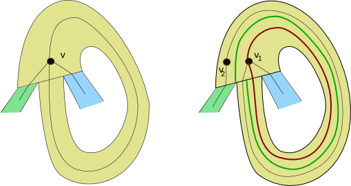
Figure 5. Vertical subdivision when digraph has a self edge.

Now suppose $\gamma$ is not a self-edge and contains $v$. Let $w_{1},\dots,w_{\ell-1}$ be the vertices in $\gamma$ other than $v$ in their induced sequential order. Let $\varepsilon_{i}$ be the edge from $w_{i-1}$ to $w_{i}$ for $i=2,\dots,\ell-1$. Then since none of the $\varepsilon_{i}$ have initial or endpoint $v$, they have unique lifts $\varepsilon_{i}^{\prime}$ in $D^{\prime}$. Since the vertical subdivision is allowable, there is one vertex, say $v_{1}^{\prime}$, above $v$ with an edge $\varepsilon_{1}^{\prime}$ from $v_{1}^{\prime}$ to $w_{2}^{\prime}$. Let $\varepsilon_{\ell}^{\prime}$ be the edge from $w_{\ell-1}^{\prime}$ to $v_{1}^{\prime}$ (cf. Figure 4). Let $\gamma^{\prime}$ be the simple cycle with edges $\varepsilon_{1}^{\prime},\dots,\varepsilon_{\ell}^{\prime}$.

Since the lift of a simple cycle is simple, the lifting map determines a well-defined map $q^{*}:C_{D}\rightarrow C_{D^{\prime}}$ that satisfies $q\circ q^{*}=\mbox{id}$ and preserves size. The commutative diagram in Lemma 3.8 implies that the images of $\sigma$ and $q^{*}(\sigma)$ in $G$ are the same, and hence their labels are the same. ∎

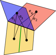
Figure 6. A switching locus.

Lemma 3.10.

Let $D^{\prime}$ be obtained from $D$ by an allowable vertical subdivision on a single $2$–cell. The set of edges of each $\sigma\in C_{D^{\prime}}{\smallsetminus}q^{*}(C_{D})$ contains exactly one matched pair.

Proof.

Since $\sigma^{\prime}\notin q^{*}(C_{D})$, the quotient map $q$ is not injective on $\sigma^{\prime}$. Thus $q(\sigma^{\prime})$ must contain two distinct edges $\varepsilon_{1},\varepsilon_{2}$ with endpoint $v$, and these have lifts $\varepsilon_{1}^{\prime}$ and $\varepsilon_{2}^{\prime}$ on $\sigma^{\prime}$. Since $\sigma^{\prime}$ is a cycle, $\varepsilon_{1}^{\prime}$ and $\varepsilon_{2}^{\prime}$ must have distinct endpoints, hence one is $v_{1}^{\prime}$ and one is $v_{2}^{\prime}$. There cannot be more than one matched pair on $\sigma^{\prime}$, since $\sigma^{\prime}$ can pass through each $v_{i}^{\prime}$ only once. ∎

Definition 3.11.

Let $D^{\prime}$ be obtained from $D$ by an allowable vertical subdivision on a single $2$–cell. Let $v$ be the vertex corresponding to the subdivided cell, and let $v_{1}^{\prime}$ and $v_{2}^{\prime}$ be its lifts to $D^{\prime}$.

For any pair of edges $\varepsilon_{1}^{\prime},\varepsilon_{2}^{\prime}$ with endpoints at $v_{1}^{\prime}$ and $v_{2}^{\prime}$ and distinct initial points $w_{1}^{\prime}$ and $w_{2}^{\prime}$, there is a corresponding pair of edges $\eta_{1}^{\prime},\eta_{2}^{\prime}$ from $w_{1}^{\prime}$ to $v_{2}^{\prime}$ and from $w_{2}^{\prime}$ to $v_{1}^{\prime}$. Write

$$\mbox{op}\{\varepsilon_{1}^{\prime},\varepsilon_{2}^{\prime}\}=\{\eta_{1}^{\prime},\eta_{2}^{\prime}\}.$$

We call the pair $\{\varepsilon_{1}^{\prime},\varepsilon_{2}^{\prime}\}$ a matched pair, and $\{\eta_{1}^{\prime},\eta_{2}^{\prime}\}$ its opposite. (See Figure 6).

Lemma 3.12.

If $\sigma^{\prime}\in C_{D^{\prime}}$ contains a matched pair, the edge-path obtained from $\sigma^{\prime}$ by exchanging the matched pair with its opposite is a cycle.

Proof.

It is enough to observe that the set of endpoints and initial points of a matched pair and its opposite are the same. ∎

Define a map $\mathfrak{r}:C_{D^{\prime}}\rightarrow C_{D^{\prime}}$ be the map that sends each $\sigma\in C_{D^{\prime}}$ to the cycle obtained by exchanging each appearance of a matched pair on $\sigma^{\prime}\in C_{D^{\prime}}$ with its opposite.

Lemma 3.13.

The map $\mathfrak{r}$ is a simplicial map of order two that preserves length and labels. It also fixes the elements of $q^{*}(C_{D})$, and changes the parity of the size of elements in $C_{D^{\prime}}{\smallsetminus}q^{*}(C_{D})$.

Proof.

The map $\mathfrak{r}$ sends cycles to cycles, and hence simplicies to simplicies. Since op has order 2, it follows that $\mathfrak{r}$ has order 2. The total number of vertices does not change under the operation op. It remains to check that the homology class of $\sigma^{\prime}$ and $\mathfrak{r}(\sigma^{\prime})$ as embedded cycles in $X$ are the same, and that the size switches parity.

There are two cases. Either the matched edges lie on a single simple cycle $\gamma^{\prime}$ or on different simple cycles $\gamma_{1}^{\prime},\gamma_{2}^{\prime}$ on $\sigma^{\prime}$.

In the first case, $\mathfrak{r}(\{\gamma^{\prime}\})$ is a cycle with 2 components $\{\gamma_{1}^{\prime},\gamma_{2}^{\prime}\}$. As one-chains we have

(6) $$\beta = \mathfrak{r}(\sigma^{\prime})-\sigma^{\prime}=\gamma_{1}^{\prime}+\gamma_{2}^{\prime}-\gamma^{\prime}=\eta_{1}^{\prime}+\eta_{2}^{\prime}-\varepsilon_{1}^{\prime}-\varepsilon_{2}^{\prime}.$$

In $X$, $\beta$ bounds a disc (see Figure 6), thus $g(\gamma^{\prime})=g(\gamma_{1}^{\prime})+g(\gamma_{2}^{\prime})$, and hence

(7) $$g(\sigma^{\prime}) = g(\mathfrak{r}(\sigma^{\prime})).$$

The one component cycle $\gamma^{\prime}$ is replaced by two simple cycles $\gamma_{1}^{\prime}$ and $\gamma_{2}^{\prime}$, and hence the size of $\sigma^{\prime}$ and $\mathfrak{r}(\sigma^{\prime})$ differ by one.

Now suppose $\sigma^{\prime}$ contains two cycles $\gamma_{1}^{\prime}$ and $\gamma_{2}^{\prime}$, one passing through $v_{1}^{\prime}$ and the other passing through $v_{2}^{\prime}$. Then $\mathfrak{r}(\sigma^{\prime})$ contains a simple cycle $\gamma^{\prime}$ in place of $\gamma_{1}^{\prime}+\gamma_{2}^{\prime}$, so the size decreases by one. By (6) we have (7) for $\sigma^{\prime}$ of this type. ∎

Proof of Proposition 3.7.

By Lemma 3.9, the quotient map $q:D^{\prime}\rightarrow D$ induces an injection of $q^{*}:C_{D}\hookrightarrow C_{D^{\prime}}$ defined by the lifting map, and this map preserves labels. We thus have

$$\theta_{X,\mathfrak{C},\psi}=1+\sum_{\sigma\in C_{D}}(-1)^{|\sigma|}g(\sigma)^{-1}=1+\sum_{\sigma^{\prime}\in q^{*}(C_{D})}(-1)^{|\sigma^{\prime}|}g(\sigma^{\prime})^{-1}.$$

The cycles in $C_{D^{\prime}}{\smallsetminus}q^{*}(C_{D})$ partition into $\sigma^{\prime},\mathfrak{r}(\sigma^{\prime})$, and by Lemma 3.13 the contributions of these pairs in $\theta_{X,\mathfrak{C}^{\prime},\psi}$ cancel with each other. Thus, we have

$$\theta_{X,\mathfrak{C}^{\prime},\psi}=1+\sum_{\sigma^{\prime}\in C_{D^{\prime}}}(-1)^{|\sigma^{\prime}|}g(\sigma^{\prime})^{-1}=1+\sum_{\sigma^{\prime}\in q^{*}(C_{D})}(-1)^{|\sigma^{\prime}|}g(\sigma^{\prime})^{-1}=\theta_{X,\mathfrak{C},\psi}.$$

∎

Definition 3.14.

Let $(X,\mathfrak{C},\psi)$ be a branched surface and $c$ a $2$–cell. Let $p,q$ be two points on the boundary $1$-chain $\partial c$ of $c$ that do not lie on the same $1$–cell of $\mathfrak{C}$. Assume that $p$ and $q$ each have the property that

1. it lies on a vertical edge, or

2. its forward flow under $\psi$ eventually lies on a vertical $1$–cell of $(X,\mathfrak{C})$.

The transversal subdivision of $(X,\mathfrak{C},\psi)$ at $(c;p,q)$ is the new branched surface $(X,\mathfrak{C}^{\prime},\psi)$ obtained from $\mathfrak{C}$ by doing the (allowable) vertical subdivisions of $\mathfrak{C}$ defined by $p$ and $q$, and doing the additional subdivision induced by adding a $1$–cell from $p$ to $q$.

Lemma 3.15.

Let $(X,\mathfrak{C},\psi)$ be a branched surface, and let $(X,\mathfrak{C}^{\prime},\psi)$ be a transversal subdivision. Then the corresponding cycle functions are the same.

Proof.

By first vertically subdividing $\mathfrak{C}$ along the forward orbits of $p$ and $q$ if necessary, we may assume that $p$ and $q$ lie on different vertical $1$–cells on the boundary of $c$. Let $v$ be the vertex of $D$ corresponding to $c$. Then $D^{\prime}$ is obtained from $D$ by substituting the vertex $v$ by a pair $v_{1}^{\prime},v_{2}^{\prime}$ that are connected by a single edge. Each edge $\varepsilon$ from $w\neq v$ to $v$ is replaced by an edge $\varepsilon^{\prime}$ from $w^{\prime}$ to $v_{1}^{\prime}$ and edge $\varepsilon$ from $v$ to $u\neq v$ is replaced by an edge from $v_{2}^{\prime}$ to $u^{\prime}$. Each edge from $v$ to itself is substituted by an edge from $v_{2}$ to $v_{1}$. The cycle complexes of $D$ and $D^{\prime}$ are the same, and their labelings are identical. Thus the cycle function is preserved. ∎

3.3. Folding

Let $(X,\mathfrak{C},\psi)$ be a branched surface with a flow. Let $c_{1}$ and $c_{2}$ be two cells with the property that their boundaries $\partial c_{1}$ and $\partial c_{2}$ both contain the segment $e_{1}e_{2}$, where $e_{1}$ is a vertical $1$–cell and $e_{2}$ is a transversal $1$–cell of $\mathfrak{C}$. Let $p$ be the initial point of $e_{1}$ and $q$ the end point of $e_{2}$. Then $p$ and $q$ both lie on vertical $1$–cells, and hence $(c_{1};p,q)$ and $(c_{2};p,q)$ define a composition of transversal subdivisions $\mathfrak{C}_{1}$ of $\mathfrak{C}$. For $i=1,2$, let $e_{3}^{i}$, be the new $1$–cell on $c_{i}$, and let $\Delta(e_{1},e_{2},e_{3}^{i})$ be the triangle $c_{i}$ bounded by the $1$–cells $e_{1},e_{2}$ and $e_{3}^{i}$.

Definition 3.16.

The quotient map $F:X\rightarrow X^{\prime}$ that identifies $\Delta(e_{1},e_{2},e_{3}^{1})$ and $\Delta(e_{1},e_{2},e_{3}^{2})$ (see Figure 7) is called the folding map of $X$. The quotient $X^{\prime}$ is endowed with the structure of a branched surface $(X^{\prime},\mathfrak{C}^{\prime},\psi^{\prime})$ induced by $(X,\mathfrak{C}_{1},\psi)$.

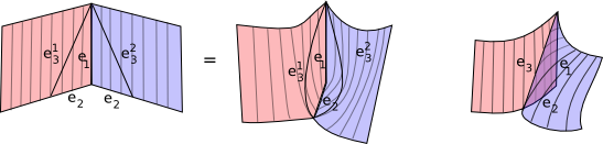
Figure 7. The left and middle diagrams depict the two $2$–cells sharing the edges $e_{1}$ and $e_{2}$; the right diagram is the result of folding.

The following Proposition is easily verified (see Figure 7).

Proposition 3.17.

The quotient map $F$ associated to a folding is a homotopy equivalence, and the semi-flow $\psi:X\times\mathbb{R}_{+}\to X$ induces a semi-flow $\psi^{\prime}:X\times\mathbb{R}_{+}\to X$.

Definition 3.18.

Given a folding map $F:X\rightarrow X^{\prime}$, there is an induced branched surface structure $(X^{\prime},\mathfrak{C}^{\prime},\psi^{\prime})$ on $X$ given by taking the minimal cellular structure on $X^{\prime}$ for which the map $F$ is a cellular map and deleting the image of $e_{2}$ if there are only two hinges containing $e_{2}$ on $X$.

Remark 3.19.

In the case that $c_{1},c_{2}$ are the only cells above $e_{2}$, then folding preserves the dual digraph $D$.

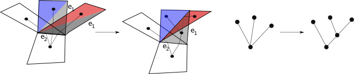
Figure 8. Effect of folding on the digraph.

Lemma 3.20.

Let $F:X\rightarrow X^{\prime}$ be a folding map, and let $(X^{\prime},\mathfrak{C}^{\prime},\psi^{\prime})$ be the induced branch surface structure of the quotient. Then

$$\theta_{X,\mathfrak{C},\psi}=\theta_{X^{\prime},\mathfrak{C}^{\prime},\psi^{\prime}}.$$

Proof.

Let $D$ be the dual digraph of $(X,\mathfrak{C},\psi)$ and $D^{\prime}$ the dual digraph of $(X^{\prime},\mathfrak{C}^{\prime},\psi^{\prime})$. Assume that there are at least three hinges containing $e_{2}$. Then $D^{\prime}$ is obtained from $D$ by gluing two adjacent half edges (see Figure 8), a homotopy equivalence. Thus, $\mathcal{C}_{\mathcal{D}}^{G}=\mathcal{C}_{\mathcal{D}^{\prime}}^{G}$, and the cycle polynomials are equal. ∎

4. Branched surfaces associated to a free group automorphism

Throughout this section, let $\phi\in\operatorname{Out}(F_{n})$ be an element that can be represented by an expanding irreducible train-track map $f:\tau\rightarrow\tau$. Let $\Gamma=F_{n}\rtimes_{\phi}\mathbb{Z}$, and $G=\Gamma^{\text{ab}}/\text{torsion}$. We shall define the mapping torus $(Y_{f},\mathfrak{C},\psi)$ associated $f$, and prove that its cycle polynomial $\theta_{Y_{f},\mathfrak{C},\psi}$ has a distinguished factor $\Theta$ with a distinguished McMullen cone $\mathcal{T}$. We show that the logarithm of the house of $\Theta$ specialized at integral elements in the cone extends to a homogeneous of degree -1, real analytic concave function $L$ on an open cone in $\textup{Hom}(G,\mathbb{R})$, and satisfies a universality property.

4.1. Free group automorphisms and train-tracks maps

In this section we give some background definitions for free group automorphisms, and their associated train-tracks following [DKL13.1]. We also recall some sufficient conditions for a free group automorphism to have an expanding irreducible train-track map due to work of Bestvina-Handel [BH92].

Definition 4.1.

A topological graph is a finite 1-dimensional cellular complex. For each edge $e$, an orientation on $e$ determines an initial and terminal point of $e$. Given an oriented edge $e$, we denote by $\overline{e}$, the edge $e$ with opposite orientation. Thus the initial and terminal points of $e$ are respectively the terminal and initial points of $\overline{e}$. An edge path on a graph is an ordered sequence of edges $e_{1}\cdots e_{\ell}$, where the endpoint of $e_{i}$ is the initial point of $e_{i+1}$, for $i=1,\dots,\ell-1$. The edge path has back-tracking if $e_{i}=\overline{e_{i+1}}$ for some $i$. The length of an edge path $e_{1}\cdots e_{\ell}$ is $\ell$.

Definition 4.2.

A graph map $f:\tau\to\tau$ is a continuous map from a graph $\tau$ to itself that sends vertices to vertices, and is a local embedding on edges. A graph map assigns to each edge $e\in\tau$ an edge path $f(e)=e_{1}\cdots e_{\ell}$ with no back tracks. Identify the fundamental group $\pi_{1}(\tau)$ with a free group $F_{n}$. A graph map $f$ represents an element $\phi\in\operatorname{Out}(F_{n})$ if $\phi$ is conjugate to $f_{*}$ as an element of $\operatorname{Out}(F_{n})$.

Remark 4.3.

In many definitions of graph map one is also allowed to collapse an edge, but for this exposition, graph maps send edges to non-constant edge-paths.

Definition 4.4.

A graph map $f\colon\thinspace\tau\rightarrow\tau$ is a train-track map if

1. $f$ is a homotopy equivalence, and

2. $f^{k}$ has no back-tracking for all $k\geq 1$, that is, for any $k\geq 1$, and edge $e$, $f^{k}(e)$ is an edge path with no back-tracking.

Definition 4.5.

Given a train-track map $f\colon\thinspace\tau\to\tau$, let $\{e_{1},\dots,e_{k}\}$ be an ordering of the edges of $\tau$, and let $D_{f}$ be the digraph whose vertices $v_{e}$ correspond to the undirected edges $e$ of $\tau$, and whose edges from $e_{i}$ to $e_{j}$ correspond to each appearance of $e_{j}$ and $\overline{e_{j}}$ in the edgepath $f(e_{i})$. The transition matrix $M_{f}$ of $D_{f}$ is the directed adjacency matrix

$$M_{f}=[a_{i,j}],$$

where $a_{i,j}$ is equal to the number of edges from $v_{e_{i}}$ to $v_{e_{j}}$.

Definition 4.6.

If $f:\tau\rightarrow\tau$ be a train-track map, the dilatation of $f$ is given by the spectral radius of $M_{f}$

$$\lambda(f)=\max\{|\mu|\ |\ \mbox{$\mu$ is an eigenvalue of $M_{f}$}\}.$$

Definition 4.7.

A train-track map $f:\tau\rightarrow\tau$ is irreducible if its transition matrix $M_{f}$ is irreducible, it is expanding if the lengths of edges of $\tau$ under iterations of $f$ are unbounded.

Remark 4.8.

A Perron-Frobenius matrix is irreducible and expanding, but the converse is not necessarily true.

Example 4.9.

Let $\tau$ be the rose with four petals $a,b,c$ and $d$. Let $f:\tau\rightarrow\tau$ be the train-track map associated to the free group automorphism

(8) $$\begin{array}[]{rcl}a&\mapsto&cdc\\ b&\mapsto&cd\\ c&\mapsto&aba\\ d&\mapsto&ab\end{array}$$

The train-track map $f$ has transition matrix

$$M_{f}=\left[\begin{array}[]{cccc}0&0&2&1\\ 0&0&1&1\\ 2&1&0&0\\ 1&1&0&0\\ \end{array}\right],$$

which is an irreducible matrix, and hence $f$ is irreducible. The train-track map is expanding, since its square is block diagonal, where each block is a $2\times 2$ Perron-Frobenius matrix. On the other hand, $f$ is clearly not PF, since no power of $M_{f}$ is positive.

Definition 4.10.

Fix a generating set $\Omega=\{\omega_{1},\dots,\omega_{n}\}$ of $F_{n}$. Then each $\gamma\in F_{n}$ can be written as a word in $\Omega$,

(9) $$\gamma=\omega_{i_{1}}^{r_{1}}\cdots\omega_{i_{\ell}}^{r_{\ell}}$$

where $\omega_{i_{1}},\dots,\omega_{i_{\ell}}\in\Omega$ and $r_{j}\in\{1,-1\}$. This representation is reduced if there are no cancelations, that is $\omega_{i_{j}}^{r_{j}}\neq\omega_{i_{j+1}}^{-r_{j+1}}$ for $j=1,\dots,\ell-1$. The word length $\ell_{\Omega}(\gamma)$ is the length $\ell$ of a reduced word representing $\gamma$ in $F_{n}$. The cyclically reduced word length $\ell_{\Omega,\mbox{\tiny cyc}}(\gamma)$ of $\gamma$ represented by the word in (9) is the minimum word length of the elements

$$\gamma_{j}=\omega_{i_{j}}^{r_{j}}\omega_{i_{j+1}}^{r_{j+1}}\cdots\omega_{i_{\ell}}^{r_{\ell}}\omega_{i_{1}}^{r_{1}}\cdots\omega_{i_{j-1}}^{r_{j-1}},$$

for $j=1,\dots,\ell-1$.

Proposition 4.11.

Let $\phi\in\operatorname{Out}(F_{n})$ be represented by an expanding irreducible train-track map $f$, and let $\gamma\in F_{n}$ be a nontrivial element. Then either $\phi$ acts periodically on the conjugacy class of $\gamma$ in $F_{n}$, or the growth rate satisfies

$$\lambda_{\Omega,\mbox{\tiny cyc}}(\gamma)=\lim_{k}\ell_{\Omega,\mbox{\tiny cyc}}(\phi^{k}(\gamma))^{\frac{1}{k}}=\lambda(f),$$

and in particular, it is independent of the choice of generators, and of $\gamma$.

Proof.

See, for example, Remark 1.8 in [BH92]. ∎

In light of Proposition 4.11, we make the following definition.

Definition 4.12.

Let $\phi\in\operatorname{Out}(F_{n})$ be an element that is represented by an expanding irreducible train-track map $f$. Then we define the dilatation of $\phi$ to be

$$\lambda(\phi)=\lambda(f).$$

Remark 4.13.

An element $\phi\in\operatorname{Out}(F_{n})$ is hyperbolic if $F_{n}\rtimes_{\phi}\mathbb{Z}$ is word-hyperbolic. It is atoroidal if there are no periodic conjugacy classes of elements of $F_{n}$ under iterations of $\phi$. By a result of Brinkmann [Br00] (see also [BF92]), $\phi$ is hyperbolic if and only if $\phi$ is atoroidal.

Definition 4.14.

An automorphism $\phi\in\operatorname{Out}(F_{n})$ is reducible if $\phi$ leaves the conjugacy class of a proper free factor in $F_{n}$ fixed. If $\phi$ is not reducible it is called irreducible. If $\phi^{k}$ is irreducible for all $k\geq 1$, then $\phi$ is fully irreducible.

Theorem 4.15 (Bestvina-Handel [BH92]).

If $\phi\in\operatorname{Out}(F_{n})$ is irreducible, then $\phi$ can be represented by an irreducible train track map, and if $\phi$ is fully irreducible, then it can be represented by a PF train track map.

Remark 4.16.

Theorem A deals with an automorphism $\phi$ that can be represented by an irreducible and expanding train-track map. It does not follow that for such an automorphism every train-track representative is expanding and irreducible. For example, consider the automorphism $\phi$ from Example 4.9. Let $\tau^{\prime}$ be a graph constructed from an edge $e$ with two distinct endpoints $v$ and $w$ by attaching at $v$ two loops labeled $a$ and $b$ and attaching at $w$ two loops $c$ and $d$. The map $f^{\prime}\colon\thinspace\tau^{\prime}\to\tau^{\prime}$ defined by equation 8 and $e\mapsto\bar{e}$ represents the same automorphism $\phi$ as in Example 4.9. However, since $e$ is invariant, the map is not irreducible and not expanding.
If we assume that $\phi$ is fully irreducible, then all train-track representatives are expanding. Indeed, let $f^{\prime}\colon\thinspace\tau^{\prime}\to\tau^{\prime}$ be a train-track representative of $\phi$. Then $f^{\prime}$ is irreducible because an invariant subgraph will produce a $\phi$-invariant free factor. It is now enough to show that some edge is expanding. Let $\alpha$ be an embedded loop in $\tau^{\prime}$. We can think of $\alpha$ as a conjugacy class in $F_{n}$. Then by proposition 4.11 either $\alpha$ is periodic or $\alpha$ grows exponentially. However, $\alpha$ cannot be periodic since $\alpha$ represents a free factor of $F_{n}$. Therefore, $\alpha$ grows exponentially, hence some edge grows exponentially and because $f^{\prime}$ is irreducible, all edges grow exponentially.

4.2. The mapping torus of a train-track map.

In this section we define the branched surface $(X_{f},\mathfrak{C}_{f},\psi_{f})$ associated to an irreducible expanding train-track map $f$.

Definition 4.17.

The mapping torus $(Y_{f},\psi_{f})$ associated to $f:\tau\rightarrow\tau$ is the branched surface where $Y_{f}$ is the quotient of $\tau\times[0,1]$ by the identification $(t,1)\sim(f(t),0)$, and $\psi_{f}$ is the semi-flow induced by the product structure of $\tau\times[0,1]$. Write

$$q:\tau\times[0,1]\rightarrow Y_{f}$$

for the quotient map. The map to the circle induced by projecting $\tau\times[0,1]$ to the second coordinate induces a map $\rho:Y_{f}\rightarrow S^{1}$.

Definition 4.18.

The $\psi_{f}$-compatible cellular decomposition $\mathfrak{C}_{f}$ for $Y_{f}$ is defined as follows. For each edge $e$, let $v_{e}$ be the initial vertex of $e$ (the edges $e$ are oriented by the orientation on $\tau$). The $0$–cells of $\mathfrak{C}_{f}$ are $q(v_{e}\times\{0\})$, the $1$–cells are of the form $s_{e}=q(v_{e}\times[0,1])$ or $t_{e}=q(e\times\{0\})$, and the $2$–cells are $c_{e}=q(e\times[0,1])$, where $e$ ranges over the oriented edges of $\tau$. For this cellular decomposition of $Y_{f}$, the collection $\mathcal{V}$ of $s_{e}$ is the set of vertical $1$–cells and the collection $\mathcal{E}$ of $1$–cells $t_{e}$ is the set of horizontal $1$–cells.

By this definition $(Y_{f},\mathfrak{C}_{f},\psi_{f})$ is a branched surface. Let $\theta_{Y_{f},\mathfrak{C}_{f},\psi_{f}}$ be the associated cycle function (Definition 3.5).

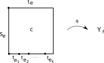
Figure 9. A cell of the mapping torus of a train-track map.

Proposition 4.19.

The digraph $D_{f}$ for the train-track map $f$ and the dual digraph of $(Y_{f},\mathfrak{C}_{f},\psi_{f})$ are the same, and we have

$$\lambda(\phi)=|\theta_{Y_{f},\mathfrak{C}_{f},\psi_{f}}^{(\alpha)}|,$$

where $\alpha:\Gamma\rightarrow\mathbb{Z}$ is the projection associated to $\phi$.

Proof.

Each $2$–cell $c$ of $(Y_{f},\mathfrak{C}_{f},\psi_{f})$ is the quotient of one drawn as in Figure 9, and hence there is a one-to-one correspondence between $2$–cells and edges of $\tau$. One can check that for each time $f(e)$ passes over the edge $e_{i}$, there is a corresponding hinge between the cell $q(e\times[0,1])$ and the cell $q(e_{i}\times[0,1])$. This gives a one-to-one correspondence between the directed edges of $D_{f}$ and the edges of the dual digraph.

Recall that $\lambda(\phi)=\lambda(f)$ is the spectral radius of $M_{f}$ (Definition 4.12). By Theorem 2.5, the characteristic polynomial of $D_{f}$ satisfies

$$P_{D_{f}}(x)=x^{m}\theta_{D_{f}}(x).$$

Each edge of $D_{f}$ has length one with respect to the map $\alpha$, and hence for each cycle $\sigma\in C_{D_{f}}$, the number of edges in $\sigma$ equals $\ell_{\alpha}(\sigma)$. It follows that $\theta_{D_{f}}(x)$ is the specialization by $\alpha$ of the cycle function $\theta_{Y_{f},\mathfrak{C}_{f},\psi_{f}}$, and we have

$$\lambda_{\mbox{PF}}(D_{f})=|P_{D_{f}}|=|\theta_{D_{f}}|=|\theta_{Y_{f},\mathfrak{C}_{f},\psi_{f}}^{(\alpha)}|.\qed$$

In the following sections, we study the behavior of $|\theta_{Y_{f},\mathfrak{C}_{f},\psi_{f}}^{(\alpha)}|$ as we let $\alpha$ vary.

4.3. Application of McMullen’s theorem to cycle polynomials

Fix a train-track map $f:\tau\rightarrow\tau$. Recall that $\theta_{f}=\theta_{Y_{f},\mathfrak{C}_{f},\pi_{f}}=1+\sum_{\sigma\in\mathcal{C}_{D_{f}}^{G}}(-1)^{|\sigma|}g(\sigma)^{-1}$. Thus the McMullen cone $\mathcal{T}_{\theta_{f}}(1)$ is given by

$$\mathcal{T}_{\theta_{f}}(1) = \{\alpha\in\textup{Hom}(G;\mathbb{R})\ |\ \alpha(g)>0,\ \mbox{for all $g\in\mbox{Supp}(\theta)$}\}$$

$$= \{\alpha\in\textup{Hom}(G;\mathbb{R})\ |\ \alpha(g)>0,\ \mbox{for all $g\in G$ such that $a_{g}\neq 0$}\}.$$

(see Definition 2.6). We write $\mathcal{T}_{f}=\mathcal{T}_{\theta_{f}}(1)$ for simplicity when the choice of cone associated to $\theta_{f}$ is understood.

Proposition 4.20.

Let $\mathcal{T}_{f}$ be the McMullen cone for $\theta_{f}$. The map

$$\delta:\textup{Hom}(G;\mathbb{R})\rightarrow\mathbb{R}$$

defined by

$$\delta(\alpha)=\log|\Theta^{(\alpha)}|,$$

extends to a homogeneous of degree $-1$, real analytic, convex function on $\mathcal{T}_{f}$ that goes to infinity toward the boundary of affine planar sections of $\mathcal{T}_{f}$. Furthermore, $\theta_{f}$ has a factor $\Theta$ with the properties:

1. for all $\alpha\in\mathcal{T}_{f}$,

   $$|\theta_{f}^{(\alpha)}|=|\Theta^{(\alpha)}|,$$

   and

2. minimality: if $\theta\in\mathbb{Z}G$ satisfies $|\theta^{(\alpha)}|=|\theta_{f}^{(\alpha)}|$ for all $\alpha$ ranging among the integer points of an open subcone of $\mathcal{T}_{f}$, then $\Theta$ divides $\theta$.

To prove Proposition 4.20 we write $G=H\times\langle s\rangle$ and identify $\theta_{f}$ with the characteristic polynomial $P_{f}$ of an expanding $H$-matrix $M_{f}$. Then Proposition 4.20 follows from Theorem 2.18.

Let

$$G=H_{1}(Y_{f};\mathbb{Z})/\mbox{torsion}=\Gamma^{\mbox{ab}}/{\mbox{torsion}},$$

and let $H$ be the image of $\pi_{1}(\tau)$ in $G$ induced by the composition

$$\tau\rightarrow\tau\times\{0\}\hookrightarrow\tau\times[0,1]\overset{q}{\rightarrow}Y_{f}.$$

Let $\rho_{*}:G\rightarrow\mathbb{Z}$ be the map corresponding to $\rho:Y_{f}\rightarrow S^{1}$.

Lemma 4.21.

The group $G$ has decomposition as $G=H\times\langle s\rangle$, where $\rho_{*}(s)=1$.

Proof.

The map $\rho_{*}$ is onto $\mathbb{Z}$ and its kernel equals $H$. Take any $s\in\rho_{*}^{-1}(1)$. Then since $s\notin H$, and $G/H$ is torsion free, we have $G=H\times\langle s\rangle$. ∎

We call $s$ a vertical generator of $G$ with respect to $\rho$, and identify $\mathbb{Z}G$ with the ring of Laurent polynomials $\mathbb{Z}H(u)$ in the variable $u$ with coefficients in $\mathbb{Z}H$, by the map $\mathbb{Z}G\rightarrow\mathbb{Z}H(u)$ determined by sending $s\in\mathbb{Z}G$ to $u\in\mathbb{Z}H(u)$.

Definition 4.22.

Given $\theta\in\mathbb{Z}G$, the associated polynomial $P_{\theta}(u)$ of $\theta$ is the image of $\theta$ in $\mathbb{Z}H(u)$ defined by the identification $\mathbb{Z}G=\mathbb{Z}H(u)$.

The definition of support for an associated polynomial $P_{\theta}$ is analogous to the one for $\theta$.

Definition 4.23.

The support of an element $P_{\theta}\in\mathbb{Z}H(u)$ is given by

$$\mbox{Supp}(P_{\theta})=\{hu^{r}\ |\ \mbox{$h$,$r$ are such that $(h,s^{r})\in\mbox{Supp}(\theta)$}\}.$$

Let $P_{\theta_{f}}\in ZH(u)$ be the polynomial associated to $\theta_{f}$. Instead of realizing $P_{\theta_{f}}$ directly as a characteristic polynomial of an $H$-labeled digraph, we start with a more natural labeling of the digraph $D_{f}$.

Let $C_{1}=\mathbb{Z}^{\mathcal{V}\cup\mathcal{E}}$ be the free abelian group generated by the positively oriented edges of $Y_{f}$, which we can also think of as 1-chains in $\mathfrak{C}^{(1)}$ (see Definition 4.18). Let $Z_{1}\subseteq C_{1}$ be the subgroup corresponding to closed 1-chains. The map $\rho$ induces a homomorphism $\rho_{*}:C_{1}\rightarrow\mathbb{Z}$.

Let $\nu:Z_{1}\rightarrow G$ be the quotient map. The map $\nu$ determines a ring homomorphism

$$\nu_{*}:\mathbb{Z}Z_{1} \rightarrow \mathbb{Z}G$$

$$\sum_{g\in Z_{1}}a_{g}g \mapsto \sum_{g\in J}a_{g}\nu(g).$$

This extends to a map from $\mathbb{Z}Z_{1}[u]$ to $\mathbb{Z}G[u]$.

Let $K_{1}\subseteq Z_{1}$ be the kernel of $\rho_{*}|_{Z_{1}}:Z_{1}\rightarrow\mathbb{Z}$. Then $H$ is the subgroup of $G$ generated by $\nu(K_{1})$. Let $\nu^{H}$ be the restriction of $\nu$ to $K_{1}$. Then $\nu^{H}$ similarly defines

$$\nu^{H}_{*}:\mathbb{Z}K_{1}\rightarrow\mathbb{Z}H,$$

the restriction of $\nu_{*}$ to $\mathbb{Z}K_{1}$, and this extends to

$$\nu^{H}_{*}:\mathbb{Z}K_{1}[u]\rightarrow\mathbb{Z}H[u].$$

Proposition 4.24.

There is a Perron-Frobenius $K_{1}$-matrix $M^{K_{1}}_{f}$, whose characteristic polynomial $P^{K_{1}}_{f}(u)\in\mathbb{Z}K_{1}[u]$ satisfies

$$P_{\theta_{f}}(u)=u^{-m}\nu^{H}_{*}P^{K_{1}}_{f}(u).$$

To construct $M^{K_{1}}_{f}$, we define a $K_{1}$-labeled digraph with underlying digraph $D_{f}$. Let $s$ be a vertical generator relative to $\rho_{*}$. Choose any element $s^{\prime}\in Z_{1}$ mapping to the vertical generator $s\in G$. Write each $s_{e}\in\mathcal{V}$ as $s_{e}=s^{\prime}k_{e}$, where $k_{e}\in K_{1}$. Label edges of the digraph $D_{f}$ by elements of $C_{1}$ as follows. Let $f(e)=e_{1}\cdots e_{r}$. Then for each $i=1,\dots,r$, there is a corresponding hinge $\kappa_{i}$ whose initial cell corresponds to $e$ and whose terminal cell corresponds to $e_{i}$. Take any edge $\eta$ on $D_{f}$ emanating from $v_{e}$. Then $\eta$ corresponds to one of the hinges $\kappa_{i}$, and has initial vertex $v_{e}$ and terminal vertex $v_{e_{i}}$. For such an $\eta$, define

$$g(\eta) = s_{e}t_{e_{1}}\cdots t_{e_{i-1}}$$

$$= s^{\prime}k_{e}t_{e_{1}}\cdots t_{e_{i-1}}$$

$$= s^{\prime}k(\eta)$$

where $k(\eta)\in K_{1}$. This defines a map from the edges $D_{f}$ to $C_{1}$ giving a labeling $\mathcal{D}_{f}^{C_{1}}$. It also defines a map from edges of $D_{f}$ to $K_{1}$ by $\eta\mapsto k(\eta)$. Denote this labeling of $D_{f}$ by $D_{f}^{K_{1}}$.

Definition 4.25.

Given a labeled digraph $\mathcal{D}^{G}$, with edge labels $g(\varepsilon)$ for each edge $\varepsilon$ of the underlying digraph $D$, the conjugate digraph $\widehat{\mathcal{D}}^{G}$ of $\mathcal{D}^{G}$ is the digraph with same underlying graph $D$, and edge labels $g(\varepsilon)^{-1}$ for each edge $\varepsilon$ of $D$.

Let $\widehat{\mathcal{D}}_{f}^{K_{1}}$ be the conjugate digraph of $\mathcal{D}_{f}^{K_{1}}$, and let $\widehat{M}^{K_{1}}_{f}$ be the directed adjacency matrix for $\widehat{\mathcal{D}}_{f}^{K_{1}}$.

Lemma 4.26.

The cycle function $\theta_{f}\in\mathbb{Z}G$ and the characteristic polynomial $\widehat{P}_{f}(u)\in\mathbb{Z}K_{1}[u]$ of $\widehat{M}^{K_{1}}$ satisfy

$$\nu_{*}^{H}(\widehat{P}_{f}(u))=u^{m}P_{\theta_{f}}(u).$$

Proof.

By the coefficient theorem for labeled digraphs (Theorem 2.14) we have

$$\widehat{P}_{f}(u)=u^{m}\theta_{\mathcal{D}_{f}^{K_{1}}}=u^{m}(1+\sum_{\sigma\in C_{D_{f}}}(-1)^{|\sigma|}k(\sigma)^{-1}u^{-\ell(\sigma)}).$$

Since $g(\sigma)=k(\sigma)s^{\ell(\sigma)}$, a comparison of $\widehat{P}_{f}$ with $\theta_{f}$ gives the desired result. ∎

Proof of Proposition 4.20.

Let $M_{f}$ be the matrix with entries in $\mathbb{Z}H$ given by taking $\widehat{M}^{K_{1}}$ and applying $\nu^{H}$ to its entries. Then the characteristic polynomial $P_{f}$ of $M_{f}$ is related to the characteristic polynomial $\widehat{P}_{f}$ of $\widehat{M}^{K_{1}}$ by

$$P_{f}(u)=\nu_{*}^{H}(\widehat{P}_{f}(u)).$$

Thus, Lemma 4.26 implies

$$P_{f}(u)=u^{m}P_{\theta_{f}}(u),$$

and hence the properties of Theorem 2.16 applied to $\widehat{P}_{f}$ also hold for $\theta_{f}$. ∎

5. The folded mapping torus and its DKL-cone

We start this section by defining a folded mapping torus and stating some results of Dowdall-Kapovich-Leininger on deformations of free group automorphisms. We then proceed to finish the proof of the main theorem.

5.1. Folding maps

In [Sta83] Stallings introduced the notion of a folding decomposition of a train-track map.

Definition 5.1 (Stallings [Sta83]).

Let $\tau$ be a topological graph, and $v$ a vertex on $\tau$. Let $e_{1},e_{2}$ be two distinct edges of $\tau$ meeting at $v$, and let $q_{1}$ and $q_{2}$ be their other endpoints. Assume that $q_{1}$ and $q_{2}$ are distinct vertices of $\tau$. The fold of $\tau$ at $v$, is the image $\tau_{1}$ of a quotient map ${\sf f}_{(e_{1},e_{2}:v)}:\tau\rightarrow\tau_{1}$ where $q_{1}$ and $q_{2}$ are identified as a single vertex in $\tau_{1}$ and the two edges $e_{1}$ and $e_{2}$ are identified as a single edge in $\tau_{1}$. The map ${\sf f}_{(e_{1},e_{2}:v)}$ is called a folding map

It is not hard to check the following.

Lemma 5.2.

Folding maps on train-tracks are homotopy equivalences.

Definition 5.3.

A folding decomposition of a graph map $f\colon\thinspace\tau\rightarrow\tau$ is a decomposition

$$f=hf_{k}\cdots f_{1}$$

where $\tau_{0}$ is the graph $\tau$ with a finite number of subdivisions on the edges, $f_{i}\colon\thinspace\tau_{i-1}\rightarrow\tau_{i}$ for $i=1,\dots,k$ are folding maps, and $h\colon\thinspace\tau_{k}\rightarrow\tau_{k}$ is a homeomorphism. We denote the folding decomposition by $(f_{1},\dots,f_{k};h)$.

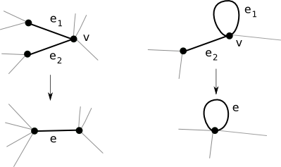
Figure 10. Two examples of folding maps.

Lemma 5.4 (Stallings [Sta83]).

Every homotopy equivalence of a graph to itself has a (non-unique) folding decomposition. Moreover, the homeomorphism at the end of the decomposition is uniquely determined.

Decompositions of a train-track map into a composition of folding maps gives rise to a branched surface that is homotopy equivalent to $Y_{f}$.

Let $f:\tau\rightarrow\tau$ be a train-track map with a folding decomposition ${\sf f}=(f_{1},\dots,f_{k};h)$, where $f_{i}:\tau_{i-1}\rightarrow\tau_{i}$ is a folding map, for $i=1,\dots,k$, $\tau=\tau_{0}=\tau_{k}$, and $h:\tau\rightarrow\tau$ is a homeomorphism.

For each $i=0,\dots,k$, define a 2-complex $X_{i}$ and semiflow $\psi_{i}$ as follows. Say $f_{i}$ is the folding map on $\tau$ folding $e_{1}$ onto $e_{2}$ at their common endpoint $v$. Let $q$ be the initial vertex of both $e_{1}$ and $e_{2}$, and $q_{i}$ the terminal vertex of $e_{i}$. Let $X_{i}$ be the quotient of $\tau_{i-1}\times[0,1]$ obtained by identifying the triangles

$$\big{[}(q,0),(q,1),(q_{1},1)\big{]}\quad\text{on}\quad e_{1}\times[0,1]$$

with

$$\big{[}(q,0),(q,1),(q_{2},1)\big{]}\quad\text{on}\quad e_{2}\times[0,1].$$

The semi-flow $\psi_{i}$ is defined by the second coordinate of $\tau_{i-1}\times[0,1]$. By the definitions, the image of $\tau_{i-1}\times\{1\}$ in $X_{i}$ under the quotient map is $\tau_{i}$.

Let $X_{\sf f}$ be the union of pieces $X_{0}\cup\cdots\cup X_{k}$ so that the image of $\tau_{i-1}\times\{1\}$ in $X_{i-1}$ is attached to the image of $\tau_{i}\times\{0\}$ in $X_{i}$ by their identifications with $\tau_{i}$, and the image of $\tau_{k}\times\{1\}$ in $X_{k}$ is attached to the image of $\tau_{0}\times\{0\}$ in $X_{0}$ by $h$.

Each $X_{i}$ has a semiflow induced by its structure as the quotient of $\tau_{i}\times[0,1]$. This induces a semiflow $\psi_{\sf f}$ on $X_{\sf f}$. The cellular structure on $X_{\sf f}$ is defined so that the $0$–cells correspond to the images in $X_{i}$ of $(q,0),(q,1),(q_{1},1)$ and $(q_{2},1)$. The transversal $1$–cells of $\mathfrak{C}_{\sf f}$ correspond to the images in $X_{i}$ of edges $[(q,0),(q_{i},1)]$, for $i=1,2$. The vertical $1$–cells of $\mathfrak{C}_{\sf f}$ are the forward flows of all the vertices of $X_{\sf f}$. The vertical and transversal $1$–cells form the boundaries of the $2$–cells of $\mathfrak{C}_{\sf f}$.

Definition 5.5 (cf. [DKL13.1]).

A folded mapping torus associated to a folding decomposition ${\sf f}$ of a train-track is the branched surface $(X_{\sf f},\mathfrak{C}_{\sf f},\psi_{\sf f})$ defined above.

Lemma 5.6.

If $(X_{\sf f},\mathfrak{C}_{{\sf f}},\psi_{{\sf f}})$ is a folded mapping torus, then there is a cellular decomposition of $X_{\sf f}$ so that the following holds:

1. The $1$–skeleton $\mathfrak{C}_{\sf f}^{(1)}$ is a union of oriented $1$–cells meeting only at their endpoints.

2. Each $1$–cell has a distinguished orientation so that the corresponding tangent directions are either tangent to the flow (vertical case) or positive but skew to the flow (diagonal case).

3. The endpoint of any vertical $1$–cell is the starting point of another vertical $1$–cell.

Proof.

The cellular decomposition of $X_{\sf f}$ has transversal $1$–cells corresponding to the folds, and vertical $1$–cells corresponding to the flow suspensions of the endpoints of the diagonal $1$–cells. ∎

5.2. Simple example

We give a simple example of a train-track map, a folding decomposition and their associated branched surfaces.

Consider the train-track in Figure 11, and the train-track map corresponding to the free group automorphism $\phi\in\operatorname{Out}(F_{2})$ defined by

$$a \mapsto ba$$

$$b \mapsto bab$$

Figure 11. Two petal rose.

Then the corresponding train-track map $f\colon\thinspace\tau\rightarrow\tau$ sends the edge $a$ over $b$ and $a$, and the edge $b$ over $b$ then $a$ then $b$. The corresponding mapping torus is shown on the left of Figure 12.

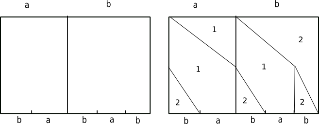
Figure 12. Mapping torus and folded mapping torus.

A folding decomposition is obtained from $f$ by subdividing the edge $a$ twice and the edge $b$ three times. The first fold identifies the entire edge $a$ with two segments of the edge $b$. This yields a train-track that is homeomorphic to the original. The second fold identifies the edge $b$ to one segment of the edge $a$. The resulting folded mapping torus is shown on the right of Figure 12. Here cells labeled with the same number are identified.

5.3. Dowdall-Kapovich-Leininger’s theorem

Recall that elements $\alpha\in H^{1}(X_{\sf f};\mathbb{R})$ can be represented by cocycle classes $z\colon\thinspace H_{1}(X_{f};\mathbb{R})\rightarrow\mathbb{R}$.

Definition 5.7.

Given a branched surface ${\sf X}=(X_{\sf f},\mathfrak{C}_{\sf f},\psi_{\sf f})$, orient the edges of $\mathfrak{C}_{\sf f}$ positively with respect to the semi-flow $\psi_{\sf f}$. The associated positive cone for ${\sf X}$ in $H^{1}(X;\mathbb{R})$, denoted $\mathcal{A}_{\sf f}$, is given by

$$\mathcal{A}_{\sf f}=\big{\{}\alpha\in H^{1}(X_{\sf f};\mathbb{R})\ \big{|}\ \mbox{there is a $z\in\alpha$ so that $z(e)>0$ for all $e\in\mathfrak{C}_{\sf f}^{(1)}$}\big{\}}.$$

Theorem 5.8 (Dowdall-Kapovich-Leininger [DKL13.1]).

Let $f$ be an expanding irreducible train-track map, ${\sf f}$ a folding decomposition of $f$ and $(X_{\sf f},\mathfrak{C}_{{\sf f}},\psi_{\sf f})$ the folded mapping torus associated to ${\sf f}$. For every integral $\alpha\in A_{\sf f}$ there is a continuous map $\eta_{\alpha}\colon\thinspace X_{\sf f}\to S^{1}$ with the following properties.

1. Identifying $\pi_{1}(X_{\sf f})$ with $\Gamma$ and $\pi_{1}(S^{1})$ with $\mathbb{Z}$, $(\eta_{\alpha})_{*}=\alpha$,

2. The restriction of $\eta_{\alpha}$ to a semiflow line is a local diffeomorphism. The restriction of $\eta_{\alpha}$ to a flow line in a $2$–cell is a non-constant affine map.

3. For all simple cycles $c$ in $X_{\sf f}$ oriented positively with respect to the flow, $\ell(\eta_{\alpha}(c))=\alpha([c])$ where $[c]$ is the image of $c$ in $G$.

4. Suppose $x_{0}\in S^{1}$ is not the image of any vertex, denote $\tau_{\alpha}:=\eta_{\alpha}^{-1}(x_{0})$. If $\alpha$ is primitive $\tau_{\alpha}$ is connected, and $\pi_{1}(\tau_{\alpha})\cong\ker(\alpha)$.

5. For every $p\in\tau_{\alpha}\cap(\mathfrak{C}_{{\sf f}})^{(1)}$, there is an $s\geq 0$ so that $\psi(p,s)\in(\mathfrak{C}_{{\sf f}})^{(0)}$.

6. The flow induces a map of first return $f_{\alpha}\colon\thinspace\tau_{\alpha}\to\tau_{\alpha}$, which is an expanding irreducible train-track map.

7. The assignment that associtates to a primitive integral $\alpha\in A_{\sf f}$ the logarithm of the dilatation of $f_{\alpha}$ can be extended to a continuous and convex function on $A_{\sf f}$.

Proof.

This is a compilation of results of [DKL13.1]. ∎

5.4. The proof of main theorem

In this section, we prove Theorem A. A crucial step to our proof is that the mapping torus ${\sf Y}=(Y_{f},\mathfrak{C}_{f},\psi_{f})$ and the folded mapping torus ${\sf X}=(X_{\sf f},\mathfrak{C}_{\sf f},\psi_{\sf f})$ both have the same cycle polynomial.

Proposition 5.9.

The cycle functions $\theta_{{\sf Y}}$ of $(Y_{f},\mathfrak{C}_{f},\psi_{f})$ and $\theta_{{\sf X}}$ of $(X_{\sf f},\mathfrak{C}_{\sf f},\psi_{\sf f})$ coincide.

Proof.

We observe that $(X_{\sf f},\mathfrak{C}_{\sf f},\psi_{\sf f})$ can be obtained from the mapping torus of the train-track map $(Y_{f},\mathfrak{C}_{f},\psi_{f})$ by a sequence of folds, vertical subdivisions and transversal subdivision, as defined in Sections 3.2 and 3.3. The reverse of these folds is shown in Figure 13.

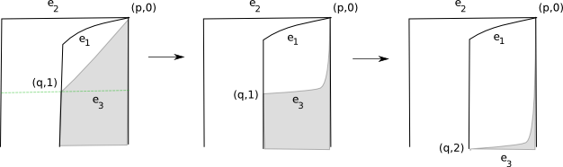
Figure 13. Vertical unfolding.

The proposition now follows from Proposition 3.7, Lemma 3.15 and Lemma 3.20, ∎

We also need to check that our theorems apply for vectors in the DLK-cone $\mathcal{A}_{\sf f}$.

Proposition 5.10.

Let $\theta_{\sf f}$ be the cycle polynomial of the DKL mapping torus. Then

$$\mathcal{A}_{\sf f}\subseteq\mathcal{T}_{\theta_{\sf f}}(1).$$

Proof.

We need to show that, for every $\sigma\in\mathcal{C}_{X_{\sf f}}$ with $|\sigma|=1$, we have $\alpha(g(\sigma))>0$. Then for all nontrivial $g\in\mbox{Supp}(\theta_{\sf f})$, we have $\alpha(g)>0$, and hence $\alpha\in\mathcal{T}_{\theta_{\sf f}}(1)=\mathcal{T}$. Let $c$ be a closed loop in $D$. The embedding of $D$ in $X_{\sf f}$ described in Def. 3.4 induces an orientation on the edges of $D$ that is compatible with the flow $\psi$. For each edge $\mu$ of $c$, item (2) in Theorem 5.8 implies $\ell(\eta_{\alpha}(\mu))>0$ and tem (3) in Theorem 5.8 implies $\alpha([c])=\ell(\eta_{\alpha}(c))=\sum_{\mu\in c}\ell(\eta_{\alpha}(\mu))>0$. ∎

Proposition 5.11.

Let $(X_{\sf f},\mathfrak{C}_{{\sf f}},\psi_{\sf f})$ be the folded mapping torus, $\theta_{\sf f}$ its cycle polynomial and $\mathcal{A}_{\sf f}$ the DKL-cone. For all primitive integral $\alpha\in A_{\sf f}$, we have

$$\lambda(\phi_{\alpha})=|\theta_{\sf f}^{(\alpha)}|$$

Proof.

Embed $\tau_{\alpha}$ in $X_{\sf f}$ transversally as in Theorem 5.8(4), and perform a vertical subdivision so that the intersections of $\tau_{\alpha}$ with $(X_{\sf f})^{(1)}$ are contained in the $0$–skeleton (we can do this by Theorem 5.8(5)). Perform transversal subdivisions to add the edges of $\tau_{\alpha}$ to the 1-skeleton. Then perform a sequence of foldings and unfoldings to move the branching of the complex into $\tau_{\alpha}$, and remove the extra edges. Denote the new branched surface by $X_{\sf f}^{(\alpha)}=(X_{\sf f},\mathfrak{C}_{{\sf f}}^{(\alpha)},\psi_{\sf f})$. These operations preserve the cycle polynomials of the respective 2-complexes, therefore we denote all of these polynomials by $\theta$ (in particular $\theta_{\sf f}=\theta$).

Let $f_{\alpha}\colon\thinspace\tau_{\alpha}\rightarrow\tau_{\alpha}$ be the map induced by the first return map, and $D_{\alpha}$ its digraph. Then $f_{\alpha}$ defines a train-track map representing $\phi_{\alpha}$, and $\lambda(\phi_{\alpha})=\lambda(D_{\alpha})$.

The (unlabeled) digraph $D_{\sf f}^{(\alpha)}$ of the new branched surface $(X_{\sf f},\mathfrak{C}_{{\sf f}}^{(\alpha)},\psi_{\sf f})$ is identical to $D_{\alpha}$. For every cycle $c$ in $D_{\alpha}$,

$$\begin{array}[]{ll}\ell(c)&=\#\text{edges in }c=\#\tau_{\alpha}\cap(X_{\sf f}^{(\alpha)})^{(1)}\\[2.84544pt] &=\ell(\eta_{\alpha}(c))=\alpha([c]).\end{array}$$

The equalities in the second line follow from Theorem 5.8(4) and (3) respectively. Thus $\ell(\sigma)=\alpha(g(\sigma))$ for every $\sigma\in C_{D_{\alpha}}$. Let $P_{\alpha}(x)$ be the characteristic polynomial of the incidence matrix associated to $D_{\alpha}$. By the coefficients theorem for digraphs (Theorem 2.5) we have:

$$P_{\alpha}(x) =x^{m}+\sum_{\sigma\in C_{D}}(-1)^{|\sigma|}x^{m-\ell(\sigma)}$$

$$=x^{m}\left(1+\sum_{\sigma\in C_{D_{\alpha}}}(-1)^{|\sigma|}x^{\alpha(g(\sigma))}\right)$$

$$=x^{m}\theta^{(\alpha)}$$

Therefore,

$$\lambda(\phi_{\alpha})=|P_{\alpha}|=|\theta^{(\alpha)}|\qed$$

We are now ready to prove our main result.

Proof of Theorem A.

Choose an expanding train-track representative $f$ of $\phi$, and a folding decomposition ${\sf f}$ of $f$. As before, let ${\sf Y}=(Y_{f},\mathfrak{C}_{f},\psi_{f})$ be the mapping torus of $f$, and ${\sf X}=(X_{{\sf f}},\mathfrak{C}_{{\sf f}},\psi_{\sf f})$ the folded mapping torus. By Proposition 5.9 their cycle function $\theta_{{\sf Y}},\theta_{{\sf X}}$ are equal, and we will call them $\theta$.

Let $\Theta$ be the minimal factor of $\theta$ defined in Proposition 4.20, and let $\mathcal{T}=\mathcal{T}_{\Theta}(1)$ be the McMullen cone. By Proposition 5.10, $A_{\sf f}\subseteq\mathcal{T}$, and by Proposition 5.11, $\lambda(\phi_{\alpha})=|\Theta^{(\alpha)}|$. By Proposition 4.20, $|\Theta_{\phi}^{(\alpha)}|=|\Theta^{(\alpha)}|$ in $\mathcal{T}$ so we have $\lambda(\alpha)=|\Theta_{\phi}^{(\alpha)}|$ for all $\alpha\in A_{\sf f}$. Item (2) of Proposition 4.20 implies part (2) of Theorem A. If ${\sf f}^{\prime}$ is another folding decomposition of another expanding irreducible train-track representative $f^{\prime}$ of $\phi$, we get another distinguished factor $\Theta_{f^{\prime}}$. Since the cones $\mathcal{T}_{\sf f}$ and $\mathcal{T}_{{\sf f}^{\prime}}$ must intersect, it follows by the minimality properties of $\Theta_{\sf f}$ and $\Theta_{f^{\prime}}$ in Proposition 4.20 that they are equal. Item (3) of Proposition 4.20 completes the proof. ∎

6. Example

In this section, we compute the cycle polynomial for an explicit example, and compare the DKL and McMullen cones.

Consider the rose with four directed edges $a,b,c,d$ and the map:

$$f=\left\{\begin{array}[]{lll}a\to&B\to&adb\\ c\to&D\to&cbd.\end{array}\right.$$

Capital letters indicate the relavent edge in the opposite orientation to the chosen one. It is well known (e.g. Proposition 2.6 in [AR]) that if $f\colon\thinspace\tau\to\tau$ is a graph map, and $\tau$ is a graph with $2m$ directed edges, and for every edge $e$ of $\tau$, the path $f^{2m}(e)$ does not have back-tracking (see Definition 4.1), then $f$ is a train-track map. One can verify that $f$ is a train-track map.

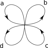
Figure 14. Four petal rose with directed edges.

The train-track transition matrix is given by

$$M_{f}=\left[\begin{array}[]{cccc}0&1&0&0\\ 1&1&0&1\\ 0&0&0&1\\ 0&1&1&1\end{array}\right].$$

The associated digraph is shown in figure 15.

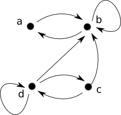
Figure 15. Digraph associated to the train-track map $f$.

The matrix $M_{f}$ is non-negative and $M_{f}^{3}$ is positive. Thus $M_{f}$ is a Perron-Frobenius matrix and $f$ is a PF train-track map, hence an expanding irreducible train-track map (see Section 4.1 for definitions). By Theorem 1.1, $\alpha_{\phi}$ has an open cone neighborhood, the DKL cone $\mathcal{A}_{\sf f}\subset\textup{Hom}(\Gamma;\mathbb{R})$ such that the primitive integral elements of $\mathcal{A}_{\sf f}$ correspond to free group automorphisms that can be represented by expanding irreducible train-track maps.

Remark 6.1.

The outer automorphism $\phi$ represented by $f$ is reducible. Consider the free factor $\langle bA,ad,ac\rangle$ then

$$f(bA)=BDAb,\quad f(ad)=BDBC=aBDAaBCA,\quad f(ac)=BD=bAad.$$

Therefore this factor is invariant up to conjugacy. Thus $\phi$ is reducible, but $f$ is a PF train-track map, and hence it is expanding and irreducible. Thus we can apply both Theorem 5.8 and Theorem A.

Identifying the fundamental group of the rose with $F_{4}$ we choose the basis $a,b,c,d$ of $F_{4}$. The free-by-cyclic group corresponding to $[f_{*}]$ has the presentation:

$$\Gamma=\langle a,b,c,d,s^{\prime}\mid a^{s^{\prime}}=B,b^{s^{\prime}}=BDA,c^{s^{\prime}}=D,d^{s^{\prime}}=DBC\rangle.$$

Let $G=\Gamma^{\text{ab}}$ and for $w\in\Gamma$ we denote by $[w]$ its image in $G$. Then

$$[a]=-[b]=[d]=-[c].$$

Thus $G=\mathbb{Z}^{2}=\langle t,s\rangle$ where $t=[a]$ and $s=[s^{\prime}]$. We decompose $f$ into four folds

$$\tau=\tau_{0}\xrightarrow{f_{1}}\tau_{1}\xrightarrow{f_{2}}\tau_{2}\xrightarrow{f_{3}}\tau_{3}\xrightarrow{f_{4}}\tau_{4}\cong\tau,$$

where all the graphs $\tau_{i}$ are roses with four petals. $f_{1}$ folds all of $a$ with the first third of $b$, to the edge $a_{1}$ of $\tau_{1}$, the other edges will be denoted $b_{1}$, $c_{1}$, $d_{1}$. $f_{1}$ folds the edge $c_{1}$ with the first third of the edge $d_{1}$. With the same notation scheme, $f_{2}$ folds the edge $c_{2}$ with half of the edge $b_{2}$ and $f_{3}$ folds the edge $a_{3}$ with half of the edge $d_{3}$. Figure 16 shows the folded mapping torus $X_{\sf f}$ for this folding sequence.

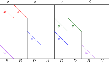
Figure 16. The complex $X$

The cell structure $\mathfrak{C}_{\sf f}$ has 4 vertices, 8 edges: $s_{1},s_{2},s_{3},s_{4},x,y,z,w$, and four 2-cells: $c_{x},c_{y},c_{z},c_{w}$. The 2-cells are sketched in Figure 17.

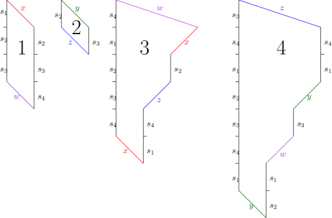
Figure 17. The discs in $X$

Let $C_{1}$ be the free abelian group generated by the edges of $X_{\sf f}$, and let $F$ be the maximal tree consisting of the edges $s_{1},s_{2},s_{3}$, then $Z_{1}\subset C_{1}$ is generated by $x,y,z,w$ and $s_{1}+s_{2}+s_{3}+s_{4}$. The quotient homomorphism $\nu\colon\thinspace Z_{1}\to G$ is given by collapsing the maximal tree and considering the relations given by the two cells. The map is given by $\nu(s_{1}+s_{2}+s_{3}+s_{4})=s$ and

$$\nu(x)=t\quad\nu(y)=\nu(z)=-t\quad\nu(w)=t+s.$$

Figure 18. The vertical diagraph is on the left and the labeled cycle complex on the right.

The dual digraph $D$ to $X$ is shown on the left of Figure 18. There are five cycles: $\omega_{13}$ and $\omega_{13}^{\prime}$ the two distinct cycles containing $1$ and $3$, $\omega_{24}$ and $\omega_{24}^{\prime}$ the two distinct cycles containing $2$ and $4$, and $\omega_{34}$ is the cycle containing $3$ and $4$. The cycle complex is shown on the right of Figure 18.

$$\begin{array}[]{ll}\theta_{f}&=1-(s^{-2}+s^{-1}t^{-1}+s^{-2}+s^{-1}t+s^{-2})+(s^{-3}t+s^{-2}+s^{-3}t^{-1}+s^{-4})\\[5.69046pt] &=1+s^{-4}-2s^{-2}-s^{-1}t^{-1}-s^{-1}t+s^{-3}t+s^{-3}t^{-1}\end{array}$$

Note that $\Theta_{\phi}$ might be a proper factor of this polynomial. However, for the sake of computing the support cone (and the dilatations of $\phi_{\alpha}$ for different $\alpha\in\mathcal{A}_{\sf f}$) we may use $\theta_{f}$.

Computing the McMullen cone: In order to simplify notation, for $\alpha\in\textup{Hom}(G,\mathbb{R})$ and $g\in G$ we denote $g^{\alpha}=\alpha(g)$. The cone $\mathcal{T}_{\phi}$ in $H^{1}(G,\mathbb{R})$ is given by

$$\begin{array}[]{ll}\mathcal{T}_{\phi}&=\{\alpha\in\textup{Hom}(G,\mathbb{R})\mid g^{\alpha}<0^{\alpha}\text{ for all }g\in\text{Supp}(\theta_{f})\}\\[5.69046pt] &=\left\{\alpha\in\textup{Hom}(G,\mathbb{R})\left|\begin{array}[]{l}(-4s)^{\alpha},(-2s)^{\alpha},(-s-t)^{\alpha}<0\\ (-s+t)^{\alpha},(-3s+t)^{\alpha},(-3s-t)^{\alpha}<0\end{array}\right\}.\right.\end{array}.$$

Therefore, the McMullen cone is

(10) $$\mathcal{T}_{\phi}=\{\alpha\in\textup{Hom}(G,\mathbb{R})\mid s^{\alpha}>0\quad\text{and}\quad|t^{\alpha}|<s^{\alpha}\}.$$

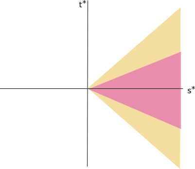
Figure 19. The McMullen cone $\mathcal{T}$ (outer) and DKL cone $\mathcal{A}_{\sf f}$ (inner).

Computing the DKL cone: We now compute the DKL cone $\mathcal{A}_{\sf f}$. A cocycle $\sf a$ represents an element in $\alpha\in\mathcal{A}_{\sf f}$ if it evaluates positively on all edges in $X_{\sf f}$. We use the notation: ${\sf a}(e)=e^{\sf a}$. Thus for ${\sf a}$ a positive cocycle: we have

$$s_{1}^{\sf a},s_{2}^{\sf a},s_{3}^{\sf a}>0$$

and

$$s_{4}^{\sf a}>0\implies s^{\sf a}-s_{1}^{\sf a}+s_{2}^{\sf a}+s_{3}^{\sf a}>0\implies s^{\sf a}>s_{1}^{\sf a}+s_{2}^{\sf a}+s_{3}^{\sf a}>0.$$

Now by considering the cell structure given by all edges in Figure 19 and recalling that $[a]=[d]=t$ and $[b]=[c]=-t$ we have:

$$x=t+s_{1}\quad w=t+s_{4}\quad y=s_{2}-t\quad z=s_{3}-t.$$

The diagonal edges $x,w$ give us:

$$0<x^{\sf a}=t^{\sf a}+s_{1}^{\sf a}\text{ and }0<w^{\sf a}=t^{\sf a}+s_{4}^{\sf a},$$

so

$$t^{\alpha}>-\frac{s_{1}^{\sf a}+s_{4}^{\sf a}}{2}>-\frac{s^{\alpha}}{2}.$$

The other diagonal edges give us

$$0<z^{\sf a}=s_{3}^{\sf a}-t^{\sf a}\text{ and }0<y^{\sf a}=s_{2}^{\sf a}-t^{\sf a},$$

hence

$$t^{\alpha}<\frac{s_{2}^{\sf a}+s_{3}^{\sf a}}{2}<\frac{s^{\alpha}}{2}.$$

We obtain the cone:

(11) $$\left\{s^{\alpha}>0~{}\text{ and }~{}|t^{\alpha}|<\frac{s^{\alpha}}{2}\right\}.$$

It is not hard to see that if $\alpha$ is in this cone we may find a positive cocycle ${\sf a}$ representing $\alpha$. Therefore $\mathcal{A}_{\sf f}$ is equal to the cone in (11) and is strictly contained in the cone $\mathcal{T}_{\phi}$ (see (10) and Figure 19).

References

- [AR] Y. Algom-Kfir and K. Rafi. Mapping tori of small dilatation irreducible train-track maps arxiv arXiv:1209.5635 [math.GT].
- [BF92] M. Bestvina and M. Feighn. A combination theorem for negatively curved groups J. Differential Geom., 35(1):85–101, 1992.
- [BNS] R. Bieri, W.D. Neumann and R. Strebel. A geometric invariant of discrete groups Inventiones Mathematicae, 90(3): 451–477, 1987.
- [BL07] S. V. Buyalo and N. D. Lebedeva. Dimensions of locally and asymptotically self-similar spaces. Algebra i Analiz, 19(1):60–92, 2007.
- [BM91] M. Bestvina and G. Mess. The boundary of negatively curved groups. J. Amer. Math. Soc., 4(3):469–481, 1991.
- [BH92] M. Bestvina and M. Handel. Train tracks and automorphisms of free groups. Ann. of Math. (2), 135(1): 1–51, 1992.
- [Br00] P. Brinkmann. Hyperbolic automorphisms of free groups. Geom. Funct. Anal., 10(5):1071–1089, 2000.
- [CR90] D. Cvetković and P. Rowlinson, The largest eigenvalue of a graph: a survey in Linear and Multilinear Algebra, 28(1-2):p.3–33,1990.
- [DKL13.1] S. Dowdall, I. Kapovich, and C. J. Leininger. Dynamics on free-by-cyclic groups. ArXiv e-prints, January 2013.
- [DKL13.2] S. Dowdall, I. Kapovich, and C. J. Leininger. McMullen polynomials and Lipschitz flows for free-by-cyclic groups. ArXiv e-prints, October 2013.
- [FLP91] A. Fathi, F. Laudenbach and V. Poénaru. Travaux de Thurston sur les surfaces. Société Mathématique de France, Paris, 1991. Séminaire Orsay, Reprint of ıt Travaux de Thurston sur les surfaces, Soc. Math. France, Paris, 1979 [ MR0568308 (82m:57003)], Astérisque No. 66-67 (1991).
- [Fri82] D. Fried. Flow equivalence, hyperbolic systems and a new zeta function for flows. Comment. Math. Helv., 57(2):237–259, 1982.
- [Gan59] F. Gantmacher. The Theory of Matrices vol. 1, Chelsea Publishing Co., 1959
- [Ger96] S. M. Gersten. Subgroups of word hyperbolic groups in dimension . J. London Math. Soc. (2), 54(2):261–283, 1996.
- [Kap13] I. Kapovich. Algorithmic detectability of iwip automorphisms, Bulletin of the London Math. Soc. to appear, arXiv:1209.3732v7 [math.GR], 2013.
- [Kit98] B. Kitchens. Symbolic dynamics: one-sided, two-sided and countable state Markov shifts, Springer, 1988
- [KLS] K. H. Ko and J. E. Los and W. T. Song. Entropies of Braids J. of Knot Theory and its Ramifications, 11(4):647–666, 2002.
- [M87] S. Matsumoto. Topological entropy and Thurston’s norm of atoroidal surface bundles over the circle J. Fac. Sci. Univ. Tokyo Sect. IA Math., 34(3):763–778, 1987.
- [McM00] C. T. McMullen. Polynomial invariants for fibered 3-manifolds and Teichmüller geodesics for foliations. Ann. Sci. École Norm. Sup. (4), 33(4):519–560, 2000.
- [McM02] C. T. McMullen. The Alexander polynomial of a 3-manifold and the Thurston norm on cohomology Ann. Sci. École Norm. Sup. (4), 35(2):153–171, 2002.
- [Neu79] W. D. Neumann. Normal subgroups with infinite cyclic quotient. Math. Sci., 4(2):143–148, 1979.
- [Oer98] U. Oertel. Affine laminations and their stretch factors. Pacific J. Math., 182(2):303–328, 1998.
- [Sta62] J. R. Stallings. On fibering certain -manifolds. In Topology of 3-manifolds and related topics (Proc. The Univ. of Georgia Institute, 1961), pages 95–100. Prentice-Hall, Englewood Cliffs, N.J., 1962.
- [Sta83] J. R. Stallings. Topology of finite graphs. Invent. Math., 71 (3): 551–565, 1983.
- [Sta68] J. R. Stallings. On torsion-free groups with infinitely many ends. Ann. of Math. (2), 88:312–334, 1968.
- [Thu86] W. P. Thurston. A norm for the homology of -manifolds. Mem. Amer. Math. Soc., 59(339):i–vi and 99–130, 1986.