Nuclear three-body problem in the complex energy plane: Complex-Scaling-Slater method

Abstract

Background: The physics of open quantum systems is an interdisciplinary area of research. The nuclear “openness” manifests itself through the presence of the many-body continuum representing various decay, scattering, and reaction channels. As the radioactive nuclear beam experimentation extends the known nuclear landscape towards the particle drip lines, the coupling to the continuum space becomes exceedingly more important. Of particular interest are weakly bound and unbound nuclear states appearing around particle thresholds. Theories of such nuclei must take into account their open quantum nature.

Purpose: To describe open quantum systems, we introduce a Complex Scaling (CS) approach in the Slater basis. We benchmark it with the complex-energy Gamow Shell Model (GSM) by studying energies and wave functions of the bound and unbound states of the two-neutron halo nucleus ⁶He viewed as an $\alpha+n+n$ cluster system.

Methods: Both CS and GSM are applied to a translationally-invariant Hamiltonian with the two-body interaction approximated by the finite-range central Minnesota force. In the CS approach, we use the Slater basis, which exhibits the correct asymptotic behavior at large distances. To extract particle densities from the back-rotated CS solutions, we apply the Tikhonov regularization procedure, which minimizes the ultraviolet numerical noise.

Results: We show that the CS-Slater method is both accurate and efficient. Its equivalence with GSM has been demonstrated numerically for both energies and wave functions of ⁶He. One important technical aspect of our calculation was to fully retrieve the correct asymptotic behavior of a resonance state from the complex-scaled (square-integrable) wave function. While standard applications of the inverse complex transformation to the complex-rotated solution provide unstable results, the stabilization method fully reproduces the GSM benchmark. We also propose a method to determine the smoothing parameter of the Tikhonov regularization.

Conclusions: The combined suite of CS-Slater and GSM techniques has many attractive features when applied to nuclear problems involving weakly-bound and unbound states. While both methods can describe energies, total widths, and wave functions of nuclear states, the CS-Slater method – if it can be applied – can provide an additional information about partial energy widths associated with individual thresholds.

I Introduction

The physics of open quantum systems spans many areas of research, ranging from optical physics to nano science, to atomic, and to nuclear physics. Of particular interest are long-lived metastable states and broad resonances: they carry rich information about localized nucleonic states confined to the nuclear interior, about the multi-channel environment of scattering and decaying states, and about the coupling between these two spaces. With exciting advances in radioactive beam experimentation worldwide, many weakly-bound isotopes inhabiting the outskirts of the nuclear landscape can now be reached; they provide a fertile territory where to study generic properties of open quantum systems Michel et al. (2010a).

To develop a microscopic theoretical framework that would unify structural and reaction-theoretical aspects of the nuclear many-body system remains a challenge. A step in this direction is the unification of bound states and resonant phenomena, often enabled by high-performance computing, and there has been an excellent progress in this area Kruppa and Nazarewicz (2004); Thompson and Nunes (2009); Deltuva et al. (2008); Baroni et al. (2013); *Navratil2; *Navratil3; Nollett et al. (2007); Hagen and Michel (2012); Papadimitriou et al. (2013); Hagen et al. (2012a); *gaute_ca48.

One possible strategy in this area is to relate the resonance parameters directly to the complex-energy eigenvalues of the effective Hamiltonian. To this end, one can solve the many-body eigenproblem with the hermitian Hamiltonian by imposing specific boundary conditions Michel et al. (2009), or one can construct a manifestly a non-hermitian effective Hamiltonian Feshbach (1962); Okołowicz et al. (2003); Volya and Zelevinsky (2006). In both cases, the eigenstates that appear below the particle threshold are bound, and the complex-energy states above the threshold represent the many-body continuum.

The GSM Michel et al. (2009) and CS Ho (1983); Moiseyev (1998); Aoyama et al. (2006) methods deal with effective non-hermitian Hamiltonians. In the GSM, one starts with a hermitian Hamiltonian and by imposing outgoing boundary conditions one ends up with a complex-symmetric Hamiltonian matrix. In the CS method, a non-Hermitian Hamiltonian appears as a result of a complex rotation of coordinates. The corresponding non-unitary transformation is characterized by a real parameter $\vartheta$. The transformed eigenstates are square integrable; this is a very attractive feature from the computational point of view. Unfortunately, since the eigenvectors depend on $\vartheta$, they cannot be directly compared with the eigenfunctions of the original Hamiltonian. To obtain the wave functions from the CS solutions, the so called-back rotation must be employed. Since in most cases the eigenproblem is solved numerically, the back-rotation constitutes an ill-posed inverse problem and a high-frequency ultraviolet noise appears Lefebvre (1988); Csótó et al. (1990). We are aware of at least two attempts Lefebvre (1992); Buchleitner et al. (1994) to overcome this problem. When the original wave function is reconstructed by means of the Padé approximation Lefebvre (1992), several calculations with different $\vartheta$ values can be carried out to perform the analytical continuation. In Ref. Buchleitner et al. (1994), special properties of the applied basis set were utilized to cure the errors of the back rotated wave function. In this work, we will present a new approach to the problem of back-rotation. Our procedure does not depend on the type of basis set used, and it is based on sound mathematical foundations.

The CS method has been successfully applied in quantum chemistry to solve many-body problems with an extremely high accuracy Bardsley (1978); Moiseyev and Corcoran (1979); Ho (1983); Moiseyev (1998); Varga et al. (2008) and also in nuclear physics, in calculations of resonance parameters Kruppa et al. (1988); Kruppa and Katō (1990) and cluster systems Aoyama et al. (2006, 1995a); *Aoyama95a; Myo et al. (2001); Kikuchi et al. (2011). In the nuclear three body calculations, mainly Jacobi coordinates have been employed. In the cluster orbital shell model Aoyama et al. (2006), besides the “V” type coordinate, also a “T” type Jacobi coordinate has been used in order to incorporate correlations. In the field of quantum chemistry, on the other hand, mainly Hylleraas-type functions Hylleraas (1929); Ruiz (2004) are used, and the achieved accuracy for the helium atom is spectacular Drake (1999); Drake et al. (2002); Korobov (2000).

In our CS calculations, we employ the Slater basis set Slater (1930), which is an approximation to the Hylleraas-type basis. The Slater wave functions have a correct asymptotic behavior, making them a perfect choice for the description of weakly-bound systems. A basis set of similar type, the Coulomb-Sturmian functions, has been recently introduced into the no-core shell model framework Caprio et al. (2012). Those functions are in fact linear superpositions of Slater orbits.

In this work, the precision of the new CS-Slater method is tested against the results of the GSM calculations. For the sake of benchmarking, we consider the energies and wave functions of the $0^{+}_{1}$ and $2^{+}_{1}$ states of ⁶He. The paper is organized as follows. Section II describes the Hamiltonian used, many-body methods, and configuration spaces employed. In Sec. III we discuss the difficulties related to the back-rotation of the CS wave function and introduce the necessary regularization scheme. Section IV presents the results for ⁶He and the details of the CS-GSM benchmarking. Finally, conclusions and future plans are contained in Sec. V.

II Models and methods

II.1 Three body Hamiltonian

For the description of the ground and excited state of ⁶He we assume a cluster ($\alpha+n+n$) picture of the nucleus. Consequently, we consider a system of three particles with masses $m_{i}$ and single particle coordinates $\bm{r}_{i}$, where $i=1,2$ for neutrons and $i=3$ for the $\alpha$-core. We introduce the relative coordinates $\bm{r}_{ij}=\bm{r}_{i}-\bm{r}_{j}$ and $r_{ij}=|\bm{r}_{ij}|$. The system Hamiltonian in the centre-of-mass frame reads:

$$H = -\frac{\hbar^{2}}{2\mu_{1}}\triangle_{\bm{r}_{13}}-\frac{\hbar^{2}}{2\mu_{2}}\triangle_{\bm{r}_{23}}-\frac{\hbar^{2}}{m_{3}}\nabla_{\bm{r}_{13}}\nabla_{\bm{r}_{23}}$$ (1)

$$+ V_{12}(\bm{r}_{12})+V_{13}(\bm{r}_{13})+V_{23}(\bm{r}_{23}),$$

where the reduced masses are:

$$\mu_{1}=\frac{m_{1}m_{3}}{m_{1}+m_{3}},~{}~{}~{}\mu_{2}=\frac{m_{2}m_{3}}{m_{2}+m_{3}}.$$ (2)

It is worth noting that the Hamiltonian (1) represents the intrinsic properties of the system, i.e., it is free from the spurious centre-of-mass motion. After introducing the single-neutron Hamiltonian,

$$H_{i3}(\bm{r})=-\frac{\hbar^{2}}{2\mu_{i}}\triangle_{\bm{r}}+V_{i3}(\bm{r})~{}~{}~{}(i=1,2),$$ (3)

the Hamiltonian (1) can be written as:

$$H=H_{13}(\bm{r}_{13})+H_{23}(\bm{r}_{23})+V_{12}(\bm{r}_{12})-\frac{\hbar^{2}}{m_{3}}\nabla_{\bm{r}_{13}}\nabla_{\bm{r}_{23}},$$ (4)

where the last term represents a two-body recoil term, which originates from the transformation to the relative coordinate frame.

II.2 Complex Scaling Method

The key element of the CS method is the complex-scaling operator $U(\vartheta)$, which transforms an arbitrary function $\chi(\bm{r}_{13},\bm{r}_{23})$ according to:

$$U(\vartheta)\chi(\bm{r}_{13},\bm{r}_{23})=e^{i3\vartheta}\chi(e^{i\vartheta}\bm{r}_{13},e^{i\vartheta}\bm{r}_{23}).$$ (5)

The transformed Shrödinger equation becomes:

$$H_{\vartheta}\Psi_{\vartheta}=E\Psi_{\vartheta},$$ (6)

where

$$H_{\vartheta}=U(\vartheta)HU(\vartheta)^{-1}$$ (7)

is a complex-scaled Hamiltonian:

$$H_{\vartheta}\ = e^{-2i\vartheta}\left(-\frac{\hbar^{2}}{2\mu_{1}}\triangle_{\bm{r}_{13}}-\frac{\hbar^{2}}{2\mu_{2}}\triangle_{\bm{r}_{23}}-\frac{\hbar^{2}}{m_{3}}\nabla_{\bm{r}_{13}}\nabla_{\bm{r}_{23}}\right)$$ (8)

$$+ V_{12}(e^{i\vartheta}\bm{r}_{12})+V_{13}(e^{i\vartheta}\bm{r}_{13})+V_{23}(e^{i\vartheta}\bm{r}_{23}).$$

The exact eigenfunctions $\Psi(\bm{r}_{13},\bm{r}_{23})$ and $\Psi_{\vartheta}(\bm{r}_{13},\bm{r}_{23})$ of the Hamiltonians (1) and (8) satisfy the following relation:

$$\Psi_{\vartheta}(\bm{r}_{13},\bm{r}_{23})=e^{i3\vartheta}\Psi(e^{i\vartheta}\bm{r}_{13},e^{i\vartheta}\bm{r}_{23})$$ (9)

or the so-called back rotation relation:

$$\Psi(\bm{r}_{13},\bm{r}_{23})=e^{-i3\vartheta}\Psi_{\vartheta}(e^{-i\vartheta}\bm{r}_{13},e^{-i\vartheta}\bm{r}_{23}).$$ (10)

According to the Aguilar-Balslev-Combes theorem Aguilar and Combes (1971); Balslev and Combes (1971), the resonant solutions of Eq. (6) are square integrable. This feature makes it possible to use bound-state methods to solve (6), including configuration interaction Ho (1983); Moiseyev (1998), Faddeev and Faddeev-Yakubovsky Lazauskas and Carbonell (2011); Lazauskas (2012), and Coupled Cluster method Bravaya et al. (2013). As illustrated in Fig. 1, the spectrum of the rotated Hamiltonian (7) consists of bound and unbound states.

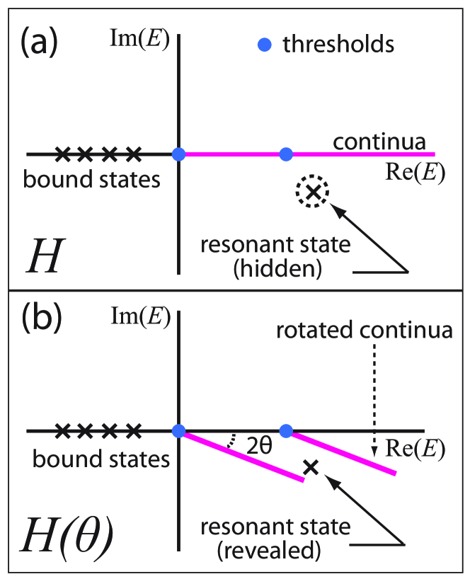
Figure 1: (Color online) Illustration of the complex scaling transformation of a many-body Hamiltonian. Bound states and many-body thresholds are invariant. Resonant eigenvalues correspond to poles of the resolvent or the $S$-matrix, are “hidden” on a sheet with $\vartheta$ = 0 (a), but are exposed if the cuts associated with many-body continua are rotated (b) Reinhardt (1982).

The continuum part of the spectrum is represented by cuts in the complex energy plane at an angle $2\vartheta$ with the real-energy axis, originating at many-body thresholds. The resonant spectrum consists of bound states lying on the negative real energy axis and positive-energy resonances. One attractive feature of the CS method is that one does not need to apply directly any boundary condition to obtain the resonant states. Through the CS transformation $U(\vartheta)$, all resonant wave functions have decaying asymptotic behavior. Even though the solution of the complex-rotated Hamiltonian $H_{\vartheta}$ is square integrable, the back-rotated wave function is an outgoing solution of the Schrödinger equation with the original Hamiltonian $H$. The back-rotation transformation, or analytical continuation, will be investigated in the following.

While the rotated non-resonant continuum states depend on the rotation angle, resonant states should be independent of $\vartheta$. In practical applications, however, Eq. (6) cannot be solved exactly and usually a truncated basis set is adopted. As a consequence, the positions of resonant states move slightly with $\vartheta$ and/or the size of the (truncated) basis. Since the dependence on $\vartheta$ is radically different for the continuum spectrum and the resonant states, there exist practical techniques to identify the resonance solutions. One of them is the so-called $\vartheta$-trajectory method: using the generalization of the virial theorem to complex energies, one finds that the resonant solution must change little with $\vartheta$ around certain value of $\vartheta=\vartheta_{\rm opt}$. In this work, we checked carefully the dependence of resonant states on both $\vartheta$ and basis parameters.

II.2.1 Slater-basis expansion

To solve the CS problem, we use a finite Slater-type basis set Slater (1930). Namely, the eigenstate of the original Hamiltonian is assumed to be

$$\Psi^{JM}(\bm{x}_{13},\bm{x}_{23})=\sum_{\{lj\}}\sum_{A}C_{A}^{\{lj\}}\chi_{A}^{\{lj\}}(r_{13},r_{23})$$

$$\times{\cal Y}_{\{lj\}}^{JMTT_{z}}(\bm{x}_{13},\bm{x}_{23}),$$ (11)

where the linear expansion coefficients $C_{A}^{\{lj\}}$ are determined by the Rayleigh-Ritz variational principle. Here $\bm{x}_{13}$, $\bm{x}_{23}$ denote the spatial and spin-isospin coordinates of first and second particle, respectively. For brevity we introduce the compact notation $\{lj\}=l_{13},j_{13},l_{23},j_{23}$. Furthermore we introduce the spin-isospin part:

$${\cal Y}_{\{lj\}}^{JMTT_{z}}(\bm{x}_{13},\bm{x}_{23})=\chi_{TT_{z}}(1,2)\times$$

$$\left[\left[{\cal Y}_{l_{13}}(\bm{r}_{13})\otimes\chi_{1/2}(1)\right]^{j_{13}}\otimes\left[{\cal Y}_{l_{23}}(\bm{r}_{23})\otimes\chi_{1/2}(2)\right]^{j_{23}}\right]^{JM},$$

where the solid spherical harmonics are ${\cal Y}_{lm}(\bm{r})=r^{l}Y_{lm}(\hat{\bm{r}})$. The symbol $[\otimes]^{JM}$ denotes the angular momentum coupling and $\hat{\bm{r}}_{ij}$ stands for the angular coordinates of $\bm{r}_{ij}$. The total isospin and single-nucleon spin functions are, respectively, denoted by $\chi_{T,T_{z}}(1,2)$ and $\chi_{1/2}(i)\ i=1,2$.

For the radial part of the wave function we use the product of Slater-type functions:

$$\chi_{A}^{\{lj\}}(r_{13},r_{23})=r_{13}^{n}e^{-\alpha r_{13}}\ r_{23}^{m}e^{-\beta r_{23}},$$ (12)

where the non-linear parameters of the basis may depend on the quantum numbers $\{lj\}$ and they are denoted by $A=\{\alpha,n,\beta,m\}$. At this point, we neglect the inter-nucleon distance $r_{12}$ in the radial part in order to span the same subspace of the Hilbert space as the GSM. (When the three-body wave function does not depend on the inter-particle distance $r_{12}$ one refers to the resulting set as the Slater basis. If all three coordinates are considered, the basis set is called Hylleraas basis.) It has been found in quantum chemistry studies Ruiz (2004) that by neglecting $r_{12}$ and by using 20-30 Slater orbits, the total energy is extremely close to the results of full Configuration Interaction calculations.

In the LS coupling, the wave function (II.2.1) can be written in the form:

$$\Psi^{JM}(\bm{x}_{13},\bm{x}_{23})=\sum_{\{lj\}}\sum_{LS}\sum_{A}C_{A}^{\{lj\}}\chi_{A}^{\{lj\}}(r_{13},r_{23})$$

$$\times\gamma_{LS}(\{lj\})\left[{\cal Y}^{L}_{l_{13}l_{23}}(\bm{r}_{13},\bm{r}_{23})\otimes\chi_{S}(1,2)\right]^{JM}$$

$$\times\chi_{TT_{z}}(1,2),$$ (13)

where

$${\cal Y}^{LM}_{l_{1}l_{2}}(\bm{r}_{1},\bm{r}_{2})=~{}~{}~{}~{}~{}~{}~{}~{}~{}~{}~{}~{}~{}$$

$$\sum_{m_{1},m_{2}}\langle l_{1}m_{1},l_{2}m_{2}|LM\rangle{\cal Y}_{l_{1},m_{1}}(\bm{r}_{1}){\cal Y}_{l_{2},m_{2}}(\bm{r}_{2})$$ (14)

are the bipolar harmonics, $\chi_{SS_{z}}(1,2)$ are coupled total spin functions, and $\gamma_{LS}(\{lj\})$ are recoupling coefficients Lawson (1980). In the case of a many-body system, the trial wave function is expanded in a many-body antisymmetric basis in a coupled or uncoupled scheme. In our formalism, we use the fully antisymmetrized wave functions expressed in both LS- and JJ-coupling schemes. The trial wave function of the CS Hamiltonian has the same form as Eq. (II.2.1):

$$\Psi_{\vartheta}^{JM}(\bm{x}_{13},\bm{x}_{23})=\sum_{\{lj\}}\sum_{A}C_{A}^{\{lj\}}(\vartheta)\chi_{A}^{\{lj\}}(r_{13},r_{23})$$

$$\times{\cal Y}_{\{lj\}}^{JMTT_{z}}(\bm{x}_{13},\bm{x}_{23}),$$

but the expansion coefficients $C_{A}^{\{lj\}}(\vartheta)$ now depend on $\vartheta$ and they are determined using the generalized variational principle.

II.2.2 Two-body matrix elements in CS

Since the CS wave function is of Slater type, one needs to develop a technique to compute two-body matrix elements (TBMEs). In the following, we shortly review a method developed in the context of atomic physics applications Éfros (1973, 1986); Drake (1978).

Since we employ the LS coupling scheme, for TBMEs we need to consider integrals of the type:

$$\langle A^{\prime}\{l^{\prime}j^{\prime}\}|V_{12}|A\{lj\}\rangle=\int d\tau\chi_{A^{\prime}}^{\{l^{\prime}j^{\prime}\}}(r_{13},r_{23}){\cal Y}^{L}_{l_{13}^{\prime}l_{23}^{\prime}}(\hat{\bm{r}}_{13},\hat{\bm{r}}_{23})^{*}$$

$$\times V_{12}(r_{12})\chi_{A}^{\{lj\}}(r_{13},r_{23}){\cal Y}^{L}_{l_{13}l_{23}}(\hat{\bm{r}}_{13},\hat{\bm{r}}_{23}).$$ (16)

To compute (II.2.2), we make a coordinate transformation to the three scalar relative coordinates $r_{12},r_{13},r_{23}$ and three Euler angles ($\Omega$) corresponding to a triangle formed by three particles. The volume element $d\tau=d\bm{r}_{13}d\bm{r}_{13}$ can be then written as $d\tau_{r}d\Omega$, where the radial volume element is given by $d\tau_{r}=dr_{12}dr_{13}dr_{23}\,r_{12}r_{13}r_{23}$, and $d\Omega$ corresponds to angular volume element involving the Euler angles. The angular integral

$$W_{l^{\prime}_{1}l^{\prime}_{2},l_{1}l_{2}}^{L}(r_{12},r_{13},r_{23})=$$

$$\int d\Omega\ {\cal Y}^{L}_{l^{\prime}_{1}l^{\prime}_{2}}(\bm{r}_{13},\bm{r}_{23})^{*}{\cal Y}^{L}_{l_{1}l_{2}}(\bm{r}_{13},\bm{r}_{23})$$ (17)

can be calculated analytically Drake (1978), and the result is:

$$W^{L}_{l^{\prime}_{1},l^{\prime}_{2},l_{1},l_{2}}(r_{12},r_{13},r_{23})=r_{13}^{l_{1}+l_{1}^{\prime}}r_{23}^{l_{2}+l_{2}^{\prime}}\times$$

$$\sum_{\lambda}A(l^{\prime}_{1},l^{\prime}_{2},l_{1},l_{2},L,\lambda)P_{\lambda}\left(\frac{r_{13}^{2}+r_{23}^{2}-r_{12}^{2}}{2r_{13}\,r_{23}}\right),$$ (18)

where

$$A(l^{\prime}_{1},l^{\prime}_{2},l_{1},l_{2},L,\lambda)=\frac{1}{2}(-1)^{L}\hat{l_{1}}\hat{l_{2}}\hat{l^{\prime}_{1}}\hat{l^{\prime}_{2}}(-1)^{\lambda}(2\lambda+1)$$

$$\times\left(\begin{array}[]{ccc}l^{\prime}_{1}&l_{1}&\lambda\\ 0&0&0\end{array}\right)\left(\begin{array}[]{ccc}l^{\prime}_{2}&l_{2}&\lambda\\ 0&0&0\end{array}\right)\left\{\begin{array}[]{ccc}l_{1}&l_{2}&L\\ l^{\prime}_{2}&l^{\prime}_{1}&\lambda\end{array}\right\},$$ (25)

with $\hat{j}\equiv\sqrt{2j+1}$. The presence of the Legendre polynomial $P_{\lambda}$ in (II.2.2) shows that the function $W^{L}_{l_{1},l_{2},l^{\prime}_{1},l^{\prime}_{2}}(r_{12},r_{13},r_{23})$ is a multinomial in the variables $r_{12},r_{13}$ and $r_{23}$. The interaction matrix element (II.2.2), can now be written in a compact form:

$$\langle A^{\prime}\{l^{\prime}j^{\prime}\}|V_{12}|A\{lj\}\rangle=$$ (26)

$$=\int_{0}^{\infty}dr_{13}\,r_{13}\int_{0}^{\infty}dr_{23}\,r_{23}\int_{|r_{13}-r_{23}|}^{r_{13}+r_{23}}dr_{12}\,r_{12}$$

$$\times\chi_{A^{\prime}}^{\{l^{\prime}j^{\prime}\}}(r_{13},r_{23})\chi_{A}^{\{lj\}}(r_{13},r_{23})$$

$$\times\,V_{12}(r_{12})W^{L}_{l^{\prime}_{13},l^{\prime}_{23},l_{13},l_{23}}(r_{12},r_{13},r_{23}).$$

Finally we determine the radial integrals. Using the functional form of the basis (12) and the dependence of the function $W^{L}_{l_{1},l_{2},l^{\prime}_{1},l^{\prime}_{2}}(r_{12},r_{13},r_{23})$ on the integration variables, it follows that the building block of the calculation is the integral:

$$I^{(\lambda)}(n_{13},n_{23})=\int_{0}^{\infty}dr_{13}\int_{0}^{\infty}dr_{23}\int_{|r_{13}-r_{23}|}^{r_{13}+r_{23}}dr_{12}\ r_{12}r_{13}^{n_{13}}r_{23}^{n_{23}}$$

$$\times V_{12}(r_{12})P_{\lambda}\left(\frac{r_{13}^{2}+r_{23}^{2}-r_{12}^{2}}{2r_{13}r_{23}}\right)\exp(-a_{13}r_{13}-a_{23}r_{23}),$$ (27)

where

$$a_{13}=\alpha^{\prime}+\alpha,~{}~{}~{}a_{23}=\beta^{\prime}+\beta,$$ (28)

and

$$n_{13}=n^{\prime}+l^{\prime}_{13}+n+l_{13}+1,~{}n_{23}=m^{\prime}+l^{\prime}_{23}+m+l_{23}+1.$$ (29)

The integral (II.2.2) can be easily calculated if the form factor of the interaction is exponential, Yukawa-like, or Coulomb Frolov and Smith (1996). For a Gaussian form factor (e.g., Minnesota force), the integral (II.2.2) is more involved and the relevant expressions are given in Appendix A.

II.3 Gamow Shell Model

The Gamow Shell Model is a complex-energy configuration interaction method Michel et al. (2009), where the many-body Hamiltonian is diagonalized in a one-body Berggren ensemble Berggren (1968) that contains both resonant and non-resonant states. The total GSM wave function is expanded in a set of basis states similar to Eq. (II.2.1). The basis functions $\psi^{(\alpha)}_{lj}(r)$ can here be represented by the eigenfunctions of a single-particle (s.p.) Hamiltonian (3) with a finite-depth potential $V(r)$:

$$\left(-\frac{\hbar^{2}}{2\mu}\triangle_{\bm{r}}+V(r)\right)\psi^{(\alpha)}_{lj}(r)\left[Y_{l}(\hat{\bm{r}})\otimes\chi_{1/2}(1))\right]^{jm}$$

$$=\epsilon_{\alpha}\psi^{(\alpha)}_{lj}(r)\left[Y_{l}({\hat{\bm{r}}})\otimes\chi_{1/2}(1))\right]^{jm}.$$ (30)

The resonant eigenstates (bound states and resonances), which correspond to the poles of the scattering $S$-matrix, are obtained by a numerical integration of the radial part of Eq. (II.3) assuming the outgoing boundary conditions:

$$\psi(r)\stackrel{{\scriptstyle r\to 0}}{{=}}r^{l+1},~{}~{}~{}~{}\psi(r)\stackrel{{\scriptstyle r\to\infty}}{{=}}H^{+}_{l}(kr),$$ (31)

where $H_{l}(kr)$ is a Hankel function (or Coulomb function for protons). The resulting s.p. energies $\epsilon_{\alpha}$ and the associated linear momenta ($k_{\alpha}=\sqrt{2me_{\alpha}}/\hbar$) are in general complex. As illustrated in Fig. 2, bound states are located on the imaginary momentum axis in the complex $k$-plane whereas the resonances are located in its forth quadrant.

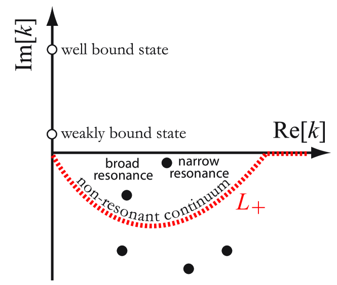
Figure 2: (Color online) Berggren ensemble in the complex-$k$ plane used to generate the s.p. basis of the GSM.

The s.p. Hamiltonian also generates non-resonant states, which are solutions obeying scattering boundary conditions. The resonant and non-resonant states form a complete set (Berggren ensemble) Berggren (1968); Lind (1993); *Lind1:

$$\sum_{b,r}|\psi_{b,r}^{\alpha}\rangle\langle\psi_{b,r}^{\alpha}|+\int_{L_{+}}dk|\psi_{k}^{\alpha}\rangle\langle\psi_{k}^{\alpha}|=1,$$ (32)

which is a s.p. basis of the GSM. In Eq. (32) $b$ (=bound) and $r$ (=resonance) are the resonant states, and the non-resonant states are distributed along a complex contour $L_{+}$. In our implementations, the continuum integral is discretized using a Gauss-Legendre quadrature. The shape of the contour is arbitrary. The practical condition is that the contour should enclose narrow resonances for a particular partial wave. Additionally, the contour is extended up to a certain momentum cut-off $k_{\rm max}$. Then convergence of results is checked with respect to both the number of shells and the s.p. cut-off. For a sufficient number of points (shells), the basis (32) satisfies the completeness relation to a very high accuracy.

The total wave function is expanded in the complete set of the Berggren’s ensemble:

$$\Psi^{JM}(\bm{x}_{13},\bm{x}_{23})=\sum_{\{lj\}}\sum_{n}\sum_{m}C_{\{lj\}}^{(n,m)}\psi^{(n)}_{l_{13}j_{13}}(r_{13})\psi^{(m)}_{l_{23}j_{23}}(r_{23})$$

$$\times{\cal Y}_{\{lj\}}^{JMTT_{z}}(\bm{x}_{13},\bm{x}_{23}).$$ (33)

Comparing Eqs. (II.3) and (II.2.1), we notice that the GSM and CS-Slater wave functions differ by their radial parts. The expansion coefficients $C^{(n)}_{lj}$’s are determined variationally from the eigenvalue problem:

$$\sum_{\alpha_{1}^{\prime}\,\alpha_{2}^{\prime}}\left(H_{\alpha_{1}\alpha_{2}\alpha_{1}^{\prime}\alpha_{2}^{\prime}}-EC_{\alpha_{1}^{\prime}\,\alpha_{2}^{\prime}}\right)=0,$$ (34)

where, $\alpha$ indices represent the s.p. $nlj$ quantum numbers. Since the basis is in general complex, $H_{\alpha_{1}\alpha_{2}\alpha_{1}^{\prime}\alpha_{2}^{\prime}}$ is a non-Hermitian complex symmetric matrix. The Berggren ensemble involves functions which are not $L^{2}$-integrable. Consequently, normalization integrals and matrix elements of operators are calculated via the “external” complex scaling technique Gyarmati and Vertse (1971).

The GSM Hamiltonian is given by Eq. (4). The s.p. potential $V(r)=V_{13}(r)=V_{23}(r)$ represents the interaction between the $\alpha$-core and the neutron, and $\mu=\mu_{1}=\mu_{2}$. The same interaction $V(r)$ is also used to generate the s.p. basis (II.3).

II.3.1 Two-body matrix elements in GSM

Once the basis is generated one needs to calculate TBMEs in the Berggren basis. Since the Berggren basis is obtained numerically, the standard Brody-Moshinsky bracket technology Moshinsky (1959); *Mosh3; *Mosh2, developed in the context of the harmonic oscillator (HO) s.p. basis, cannot be employed. To overcome this difficulty, we expand the NN interaction in a truncated HO basis Hagen et al. (2006):

$$V_{NN}=\sum_{\alpha\beta\gamma\delta}^{N_{\rm max}}|\alpha\beta\rangle\langle\alpha\beta|V_{NN}|\gamma\delta\rangle\langle\gamma\delta|.$$ (35)

The TBMEs in the Berggren ensemble are given by:

$$\langle\widetilde{ab}|V_{NN}|cd\rangle=\sum_{\alpha\beta\gamma\delta}^{n_{\rm max}}\langle\widetilde{ab}|\alpha\beta\rangle\langle\alpha\beta|V_{NN}|\gamma\delta\rangle\langle\gamma\delta|cd\rangle,$$ (36)

where the Latin letters denote Berggren s.p. wave functions and Greek letters – HO states. Due to the Gaussian fall-off of HO states, no external complex scaling is needed for the calculation of the overlaps $\langle\alpha\beta|ab\rangle$. Moreover, matrix elements $\langle\alpha\beta|V_{NN}|\gamma\delta\rangle$ of the NN interaction in the HO basis can be conveniently calculated using the Brody-Moshinsky technique Moshinsky (1959); *Mosh3; *Mosh2. This method of treating the TBMEs of the interaction is similar to the technique based on a separable expansion of the potential Gyarmati and Kruppa (1986). The HO basis depends on the oscillator length $b$, which is an additional parameter. However, as it was demonstrated in Refs. Hagen et al. (2006); Michel et al. (2010b), GSM eigenvalues and eigenfunctions converge for a sufficient number of $n_{\rm max}$, and the dependence of the results on $b$ is negligible. We shall return to this point in Sec. IV.1 below.

II.3.2 Model space of GSM

The CS and GSM calculations for the 0⁺ g.s. of ⁶He have been performed in a model space of four partial waves: $p_{3/2}$, $p_{1/2}$, $s_{1/2}$, and $d_{5/2}$. The Berggren basis consists of the 0$p_{3/2}$ resonant state, which is found at an energy of $0.737-i0.292$ MeV, and the $p_{3/2}$ complex contour in order to satisfy the Berggren’s completeness relation. The remaining partial waves $p_{1/2}$, $s_{1/2}$, and $d_{5/2}$ are taken along the real axis. Each contour is discretized with sixty points; hence, our one-body space consists of 241 neutron shells total. Within such a basis, results are independent on the contour extension in the $k$-space. For the present calculation we used a $k_{\rm max}=3.5$ fm^-1. The finite range Minnesota interaction was expanded in a set of HO states. For the g.s., when a relatively large set of HO quanta is used, the dependence of the results on the HO parameter $b$ is negligible. We took $b=2$ fm and we used all HO states with up to $n_{\rm max}=18$ radial nodes. Since the $s$ wave enters the Berggren ensemble, in order to satisfy the Pauli principle between core and valence particles we project out the Pauli forbidden $0s_{1/2}$ state ($b=1.4$ fm) using the Saito orthogonality-condition model Saito (1969).

For the excited unbound 2⁺ state of ⁶He we limit ourselves to a $p_{3/2}$ model space. As concluded in Ref. Papadimitriou et al. (2011), the structure of this state is dominated by a $(p_{3/2})^{2}$ parentage. Moreover, in this truncated space the neutron radial density becomes less localized since the 2⁺ becomes less bound when the model space is increased. The width of this state increases from $\sim$250 keV in the ($p_{3/2}$, $p_{1/2}$, $s_{1/2}$, $d_{5/2}$) space to $\sim$580 keV in the truncated space of $p_{3/2}$ waves. Dealing with a broader resonance facilitates benchmarking with CS back-rotation results and helps pinning down dependence on HO parameters in GSM calculations. The $p_{3/2}$ continuum was discretized with a maximum of 60 points. This ensures fully converged results with respect to the Berggren basis (both the number of discretization points and $k_{\rm max}$).

III Back rotation: from Complex Scaling to Gamow states

Even if the energies of resonant states in CS and GSM are the same, the wave functions are different (see Eqs. (9) and (10)). This implies that the respective expectation values of an observable $\hat{O}$ in states $\Psi(\bm{r}_{13},\bm{r}_{23})$ and $\Psi_{\vartheta}(\bm{r}_{13},\bm{r}_{23})$ cannot be compared directly. Moreover, when the wave function $\Psi_{\vartheta}(\bm{r}_{13},\bm{r}_{23})$ is used, one has to deal with the transformed operator:

$$\hat{O}_{\vartheta}=U(\vartheta)\hat{O}U(\vartheta)^{-1}.$$ (37)

In some cases, it is straightforward to derive the transformed operator. For instance, in the calculation of the root-mean-square radius, the transformed operator is $e^{2i\vartheta}\bm{r}_{13}^{2}+e^{2i\vartheta}\bm{r}_{23}^{2}$. The transformed recoil operator is given by $-e^{-2i\vartheta}\frac{\hbar^{2}}{m_{3}}\nabla_{\bm{r}_{13}}\nabla_{\bm{r}_{23}}$, and the angular correlation function is the mean value of the operator $\delta(\theta_{12}-\theta)$, where $\theta_{12}$ is the angle between the vectors $\bm{r}_{13}$ and $\bm{r}_{23}$. For the radial density, the situation is not that simple and we shall discuss this point in the following.

In order to retrieve the Gamow wave function of the original Schrödinger equation, it is tempting to carry out a direct back-rotation of the CS wave function (II.2.1):

$$e^{-i3\vartheta}\sum_{\{lj\}}\sum_{A}C_{A}^{\{lj\}}(\vartheta)\chi_{A}^{\{lj\}}(e^{-i\vartheta}r_{13},e^{-i\vartheta}r_{23})$$

$$\times{\cal Y}_{\{lj\}}^{JMTT_{z}}(\bm{x}_{13},\bm{x}_{23}).$$ (38)

It turns out, however, that this method is numerically unstable. Even for one particle moving in a potential well, the direct back-rotation leads to unphysical large oscillations in the wave function Csótó et al. (1990); Lefebvre (1988). To prevent this, a proper regularization procedure needs to be applied Fu et al. (2008, 2009).

The radial density is defined as the mean value of the operator:

$$\frac{1}{2}\left[\delta(r_{13}-r)+\delta(r_{23}-r)\right].$$ (39)

Using the CS wave function (III) and the Slater-type radial basis functions (12), the density can be casted into the form:

$$\rho_{\vartheta}(r)=r^{2}\sum_{j}C_{j}(\vartheta)r^{n_{j}}\exp(-a_{j}r),$$ (40)

where C${}_{j}(\vartheta)$ are related to the linear expansion parameters (II.2.1), obtained from the diagonalization of the complex scaled Hamiltonian (6). If we consider the direct back-rotated wave function, the radial density is given by:

$$\rho^{\rm back}_{\vartheta}(r)=e^{-i\vartheta}\tilde{\rho}_{\vartheta}(e^{-i\vartheta}r),$$ (41)

where

$$\tilde{\rho}_{\vartheta}(r)=r^{2}\sum_{j}C_{j}(\vartheta)r^{n_{j}}\exp(-a_{j}r).$$ (42)

The factor $r^{2}$ comes from the volume element when the Dirac-delta function in (39) is integrated. We shall see that the density calculated in this way leads to extremely inaccurate results. In the following, we briefly show how to calculate the density of the original Gamow state using the CS wave function. Illustrative numerical examples will be presented in Sec. IV.2.

We may consider Eq. (42) as a definition of a function defined along the non negative real axis and $\tilde{\rho}_{\vartheta}(e^{-i\vartheta}r)$ can be viewed as an attempt to extend (42) into the complex plane. However, since the coefficients $C_{i}(\vartheta)$ obtained numerically are not accurate enough, and moreover the Slater expansion is always truncated, the analytical continuation of $\tilde{\rho}_{\vartheta}$ is not a simple task. To find a stable solution, we apply a method based on the theory of Fourier transformations. We first extend $\tilde{\rho}_{\vartheta}(r)$ from $(0,\infty)$ to $(-\infty,\infty)$ by means of the mapping:

$$f_{\vartheta}(x)=\tilde{\rho}_{\vartheta}(r_{0}e^{-x}).$$ (43)

The Fourier transform of (43) is:

$$\hat{f}_{\vartheta}(\xi)=\frac{1}{\sqrt{2\pi}}\int_{-\infty}^{\infty}e^{-ix\xi}f_{\vartheta}(x)\,dx=$$

$$=\frac{1}{\sqrt{2\pi}}\sum_{j}C_{j}(\vartheta)r_{0}^{n_{j}+2}\frac{\Gamma(n_{j}+2+i\xi)}{(r_{0}a_{j})^{n_{j}+2+i\xi}},$$ (44)

where $\xi$ and $x$ are dimensionless variables.

Usually, $\hat{f}_{\vartheta}$ is determined with an error, which results in the appearance of high-frequency oscillations in $f_{\vartheta}$. Now we shall apply the Tikhonov smoothing Tikhonov (1963) to $f_{\vartheta}(x+iy)$. To this end, we perform the analytical continuation of $f_{\vartheta}(x)$ to the complex plane $x+iy$ Fu et al. (2008):

$$f_{\vartheta}(x+iy)=\frac{1}{\sqrt{2\pi}}\int_{-\infty}^{\infty}d\xi\,e^{-i(x+iy)\xi}\hat{f}_{\vartheta}(\xi).$$ (45)

The Tikhonov regularization Fu et al. (2009) removes the ultraviolet noise in (45) by introducing a smoothing function:

$$f^{reg}_{\vartheta}(x+iy) = \frac{1}{\sqrt{2\pi}}\int_{-\infty}^{\infty}e^{-i(x+iy)\xi}$$ (46)

$$\times \frac{\hat{f}_{\vartheta}(\xi)}{1+\kappa e^{-2y\xi}}d\xi,$$

where $\kappa$ is the Tikhonov smoothing parameter. In the actual calculation we take $x=-\ln(r/r_{0})$, $y=\vartheta$, and $r_{0}=1$ fm.

IV Results

For the neutron-core interaction we employ the KKNN potential Kanada et al. (1979) and the interaction between the valence neutrons is approximated by the Minnesota force Thompson et al. (1977). We study the convergence properties of the CS-Slater method not only for energies of $0^{+}_{1}$ and $2^{+}_{1}$ of ⁶He and individual energy components, but also for radial properties and spatial correlations.

IV.1 Energies

According to (4) the total Hamiltonian of ⁶He is the sum of one-body terms $H_{13}(\bm{r}_{13})+H_{23}(\bm{r}_{23})$ and two-body terms $-\frac{\hbar^{2}}{m_{3}}\nabla_{\bm{r}_{13}}\nabla_{\bm{r}_{23}}+V_{12}(\bm{r}_{12})$.

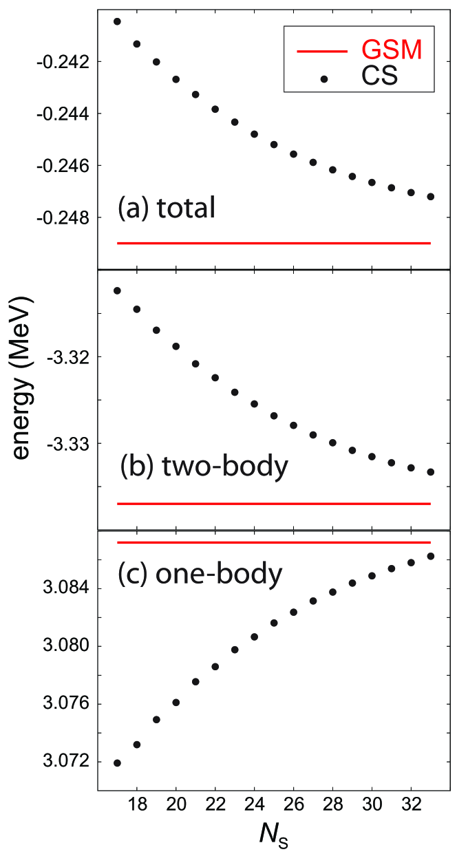
Figure 3: (Color online) Convergence of the ⁶He total g.s. energy, two-body, and one-body terms, with respect to the number of Slater orbitals $N_{\rm S}$ for $\alpha=\beta=0.8$.

Figure 3 illustrates the convergence of the CS energies with respect to the basis size $N_{\rm S}\geq n+m$ (see Eq. (12) for notation). A similar type of restriction was used in Refs. Drake (1999); Drake et al. (2002) in order to avoid the linear dependence of the basis functions. For the non-linear parameters of the Slater basis we assumed the value $\alpha=\beta=0.8$. The dependence on the Slater basis parameter $\alpha$ is shown in Fig.4 for $N_{\rm S}=27$.

In Figs. 3 and 4, horizontal solid lines correspond to GSM results. The maximum difference between CS and GSM energies is of the order of 2 keV for the total energy, two-body, and one-body terms. As can be seen in Fig. 4, two-body and one-body terms have no minima with respect to $\alpha$. This is expected as it is the total energy that that is supposed to exhibit a variational minimum, not its individual contributions.

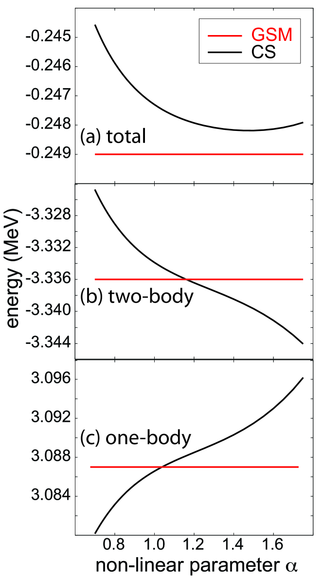
Figure 4: (Color online) Similar as in Fig. 3 but versus the non-linear Slater basis parameter $\alpha=\beta$ for $N_{\rm S}=27$.

The two and one body terms coincide with the GSM result for a slightly different variational parameter ($\alpha\sim 1.1$) than the one that corresponds to the minimum of the total energy ($\alpha=1.5$). Nevertheless, the difference at the minimum is very small, of the order of 2 keV.

Table 1 displays the energy budget for the bound g.s. configuration of ⁶He in GSM and CS methods. Even though it is not necessary to use CS for a bound state, we also show values for $\vartheta$ = 0.2, for the reasons that will be explained later in Sec. IV.2. In this case, the expectation value of the transformed operator $\hat{O}_{\vartheta}=U(\vartheta)\hat{O}U(\vartheta)^{-1}$ was computed. It is seen that the excellent agreement is obtained between GSM and both CS variants not only for the total energy but also for all Hamiltonian terms.

Table 1: Energy decomposition of ⁶He g.s. Values are in MeV.

$\langle\hat{O}\rangle$	GSM	CS ($\vartheta=0$)	CS ($\vartheta=0.2$)
$\langle\,\hat{H}\rangle$	$-$0.249	$-$0.247	$-0.24{\color[rgb]{0,0,1}7}+i1.1\times 10^{-3}$
$\langle\,\hat{T}\rangle$	24.729	24.731	$24.7{\color[rgb]{0,0,1}33}-i7.27\times 10^{-3}$
$\langle\,V_{c-n}\rangle$	$-$21.642	$-$21.645	$-21.64{\color[rgb]{0,0,1}7}+i4.76\times 10^{-3}$
$\langle\,V_{nn}\rangle$	$-$2.711	$-$2.710	$-2.71{\color[rgb]{0,0,1}0}+i3.11\times 10^{-3}$
$\langle\,\frac{\vec{p_{1}}\cdot\vec{p_{2}}}{m_{3}}\rangle$	$-$0.625	$-$0.623	$-0.62{\color[rgb]{0,0,1}3}+i5.04\times 10^{-3}$

We now move on to the 2⁺ unbound excited state of ⁶He. To assess the accuracy of computing this state in GSM, we test the sensitivity of calculations to the HO expansion (36). It is worth noting that in the GSM only the two-body interaction and recoil term are treated within the HO expansion. The kinetic term is calculated in the full Berggren basis; hence, the system maintains the correct asymptotic behavior. Moreover, for the $2^{+}$ state in the $p_{3/2}$ model space, the recoil term vanishes.

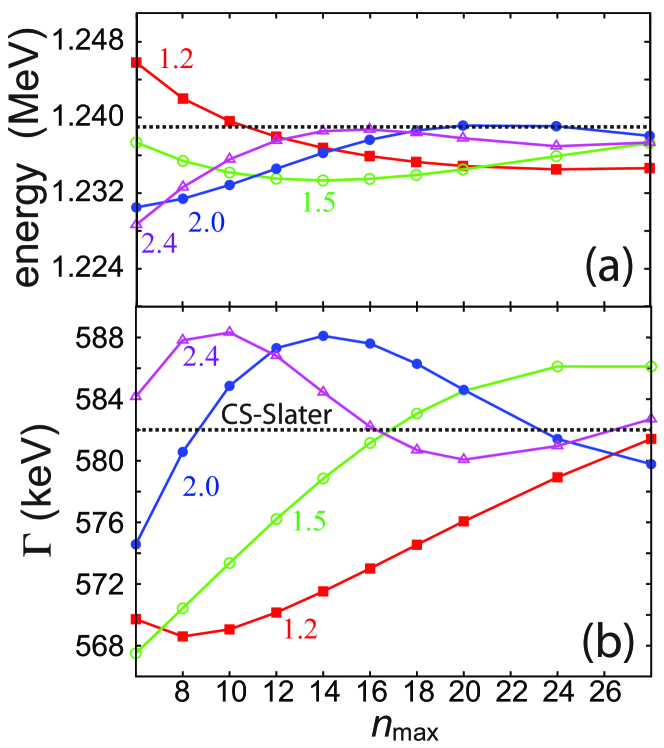
Figure 5: (Color online) Dependence of the energy (a) and width (b) of the unbound 2${}^{+}_{1}$ state in ⁶He calculated with GSM on the HO expansion parameters $n_{\rm max}$ and $b$ (=1.2, 1.5, 2.0, and 2.4 fm) in Eq. (36). The CS-Slater result is marked by a dotted line.

The resonance position in the CS-Slater method is determined with the $\vartheta$-trajectory method. Figure 5 displays the result of our tests. Overall, we see a weak dependence of the energy and width of the 2⁺ state predicted in GSM on the HO expansion parameters $n_{\rm max}$ and $b$. The increase of $n_{\rm max}$ from 6 to 28 results in energy (width) change of $\sim$20 keV ($\sim$10 keV). With increasing $n_{\rm max}$, the results become less dependent on the oscillator length $b$. For the real part of the energy, there appears some stabilization at large values of $n_{\rm max}$. but the pattern is different for different values of $b$. The most stable results are obtained with $b=2$ fm, where we find a broad plateau for both the energy and the energy modulus Moiseyev et al. (1978); Moiseyev (1998); Rotureau et al. (2009) for $n_{\rm max}>16$. We adopt the value of $b_{\rm opt}=2$ fm for the purpose of further benchmarking.

The pattern for the width is similar, with no clear plateau but very small differences at large $n_{\rm max}$. Such a behavior is not unexpected. While the variational arguments do not apply to the interaction but to the trial wave function Moiseyev et al. (1978); Moiseyev (1998); Rotureau et al. (2009), one can demonstrate Hagen et al. (2006); Michel et al. (2010b) that while the matrix elements exhibit weak converge with $n_{\rm max}$, eigenvectors and energies show strong convergence. However, the actual convergence is very slow for broad resonant states.

Based on our tests presented in Fig. 5 we conclude that the numerical error of GSM, due to HO expansion, on the energy and width of the $2^{+}_{1}$ resonance in ⁶He is $\sim 2$ keV. This accuracy is more than needed to carry out the CS-GSM benchmarking.

Table 2 displays the energy budget for the unbound 2${}^{+}_{1}$ state of ⁶He.

Table 2: Similar to Table 1 but for the 2${}^{+}_{1}$ resonance. In GSM calculations, we used $b_{\rm opt}=2$ fm and $n_{\rm max}=20$ (GSM_I) and $n_{\rm max}=24$ (GSM_II). The optimal scaling angle $\vartheta_{\rm{\rm opt}}=0.43$ was obtained with the $\vartheta$-trajectory method.

$\langle\hat{O}\rangle$	CS ($\vartheta$ = $\vartheta_{\rm{\rm opt}}$)	GSMI	GSMII
$\langle\,\hat{H}\rangle$	$1.239-i0.291$	$1.239-i0.29{\color[rgb]{0,0,1}2}$	$1.239-i0.29{\color[rgb]{0,0,1}0}$
$\langle\,\hat{T}\rangle$	$17.340-i7.949$	$17.3{\color[rgb]{0,0,1}11}-i7.{\color[rgb]{0,0,1}825}$	$17.{\color[rgb]{0,0,1}221}-i7.{\color[rgb]{0,0,1}766}$
$\langle\,V_{c-n}\rangle$	$-15.831+i7.408$	$-15.8{\color[rgb]{0,0,1}05}+i7.{\color[rgb]{0,0,1}288}$	$-15.{\color[rgb]{0,0,1}717}+i7.{\color[rgb]{0,0,1}231}$
$\langle\,V_{nn}\rangle$	$-0.270+i0.250$	$-0.2{\color[rgb]{0,0,1}67}+i0.2{\color[rgb]{0,0,1}44}$	$-0.2{\color[rgb]{0,0,1}65}+i0.2{\color[rgb]{0,0,1}44}$

We show two variants of GSM calculations in which the interaction was expanded in a HO basis with $b_{\rm opt}=2$ fm and $n_{\rm max}$ = 20 (GSM_I) and 24 (GSM_II). The real parts of the total energy are identical in both methods up to the third digit, and the imaginary parts up to second digit. For the other parts of the Hamiltonian, results are not as precise as for the g.s. calculations in Table 1; nevertheless, we obtain an overall satisfactory agreement. It is encouraging, however, that for the total complex energy the agreement is excellent. The benchmarking results presented in this section demonstrate the equivalence of GSM and CS-Slater methods for energies of bound and unbound resonance states. In the following, we shall see that this equivalence also holds for the many-body wave functions.

IV.2 One-body densities

To assess the quality of wave functions calculated with GSM and CS-Slater, we first calculate the radial one-neutron density of the g.s. of ⁶He. Figure 6 shows that both methods are consistent with each other and they correctly predict exponential fall-off at large distances. We also display the one-neutron density obtained with the radial part of the wave function (II.2.1) spanned by the radial HO basis states with $b=2$ fm and $n_{\rm max}=18$. As expected, the HO result falls off too quickly at very large distances due to the incorrect asymptotic behavior.

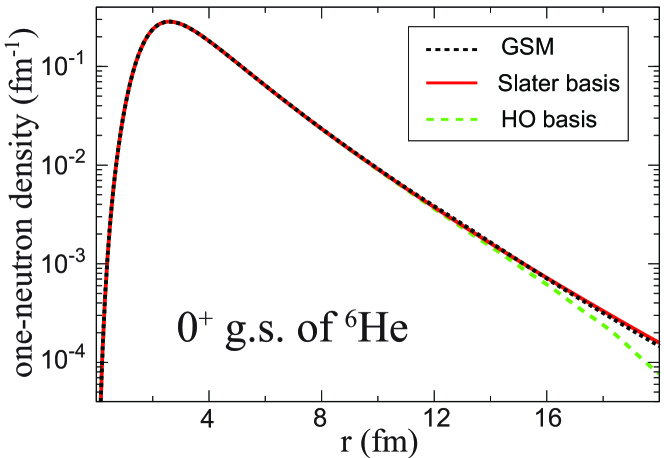
Figure 6: (Color online) Ground-state one-neutron radial density in ⁶He predicted with GSM, CS-Slater, and HO basis sets.

The g.s. of ⁶He is a bound state; hence, its description does not require a complex rotation of the Hamiltonian. Nevertheless, it is instructive to study the effect of CS on its radial properties.

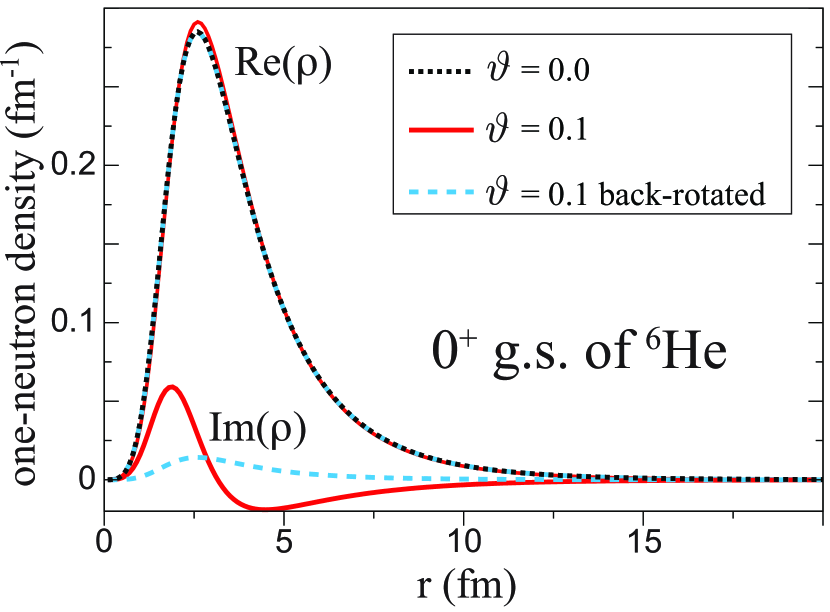
Figure 7: (Color online) Ground-state one-neutron radial density in ⁶He predicted in CS-Slater using $\vartheta=0$ (dotted line) and 0.1 (solid line). The back-rotated $\vartheta=0.1$ result is marked by a dashed line.

Figure 7 shows the g.s. one-neutron density obtained in CS-Slater using $\vartheta=0.1$. For comparison we also display the unscaled ($\vartheta=0$) density of Fig. 6. We see that the one-particle density is $\vartheta$-dependent and for $\vartheta>0$ it acquires an imaginary part. Since the integral of the density is normalized to 1, the integral of the imaginary part should be zero. This was checked numerically to be indeed the case. Since the back-rotated density should be equivalent to the unscaled or GSM one, its imaginary part should vanish. However, as seen in Fig. 7, the back-rotated density at $\vartheta=0.1$ is nonzero. This is indicative of serious problems with back-rotation in CS, if this method is applied directly Lefebvre (1988); Csótó et al. (1990).

In order to investigate back-rotation in more detail, we consider the $2^{+}_{1}$ resonance in ⁶He. As in Sec. IV.1, we limit ourselves to a $p_{3/2}$ model space to better see the effect of back-rotation; by adding more partial waves, the $2^{+}$ state becomes more localized and the CS density resembles the GSM result.

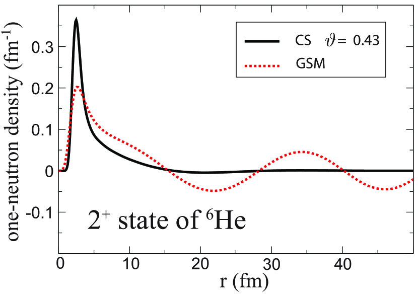
Figure 8: (Color online) Real part of one-neutron radial density for the unbound 2⁺ state in ⁶He obtained in GSM (solid line) and CS-Slater ($\vartheta_{\rm{\rm opt}}=0.43$).

The one-body density derived from the rotated CS solution is very different from the GSM density, see Fig. 8. As the theory implies, the CS density is localized, and the degree of localization increases with $\vartheta$ Lefebvre (1988). To compare with the GSM density, which has outgoing asymptotics, we need to back-rotate the CS radial density.

The comparison of the back-rotated CS-Slater and GSM 2⁺-state densities is presented in Figs. 9 and 10. Here the problem with the back-rotated CS density is far more pronounced than for the g.s. case shown in Fig. 7: at $r>2$ fm, the real part of the back-rotated density exhibits unphysical oscillations. The magnitude of those oscillations grows with $\vartheta$, even if the basis size is increased. The situation is even worse for the imaginary part of the density, which does not resemble the GSM density at $r>1$ fm.

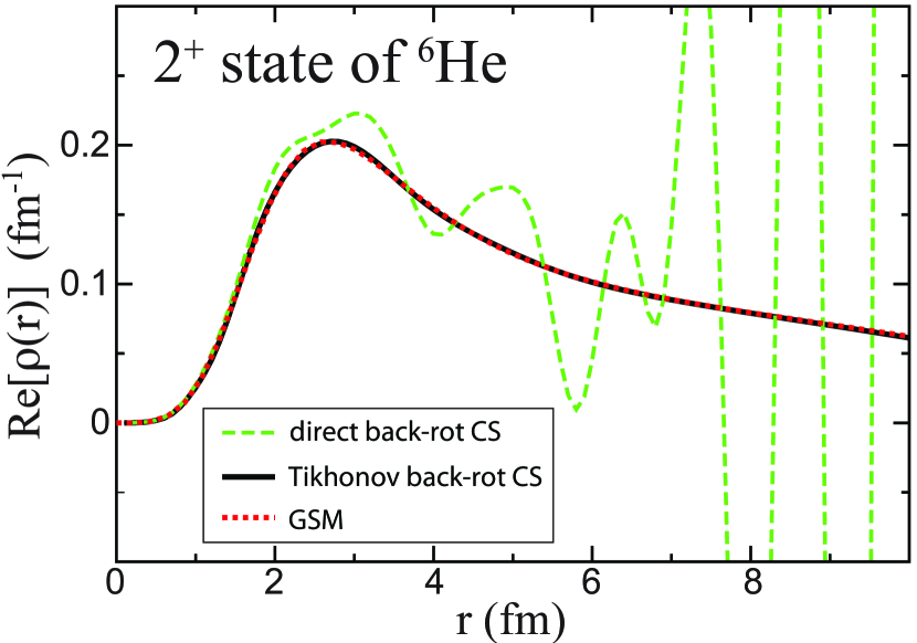
Figure 9: (Color online) Real part of one-neutron radial density for the unbound 2⁺ state in ⁶He obtained in the back-rotated (dashed line) and Tikhonov-regularized-back-rotated (solid) CS-Slater method at $\vartheta_{\rm{\rm opt}}$. The GSM density is marked by a dotted line.

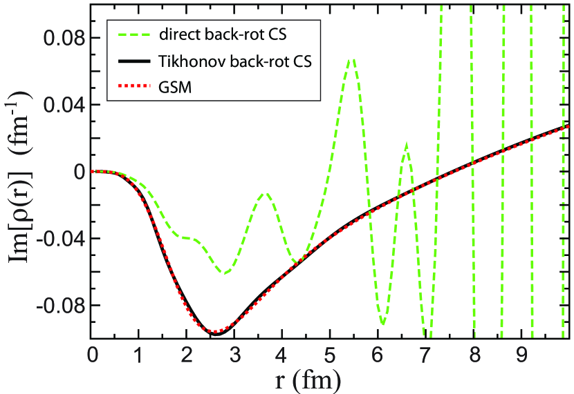
Figure 10: (Color online) Similar to Fig. 9 but for the imaginary part of the density.

The numerical instability of the back-rotated CS wave functions is an example of an ill-posed inverse problem Tikhonov and Goncharsky (1987). The amplitudes of the wave function (42) are determined numerically, and the associated errors are amplified during the back-rotation (41) causing instabilities seen in Figs. 9 and 10. Consequently, one needs a regularization method to minimize the errors that propagate from the coefficients to the solution. In this paper, we apply the Fourier analytical continuation and Tikhonov regularization procedure Tikhonov (1963); Fu et al. (2009) described in Sec. III.

We first investigate the Fourier transform (45), which provides us with an analytical continuation of the density. It is understood that if one performs the integral in the full interval $(-\infty,\infty)$, the analytically-continued density would also exhibit unwanted oscillations. Indeed, at large negative values of $\xi$ in (45), the exponent may become very large amplifying numerical errors of the Fourier transform $\hat{f}_{\vartheta}(\xi)$ and causing numerical instabilities. For this reason we cut the lower range of $\xi$ in (45) to obtain the expression for the Fourier-regularized function:

$$f_{\vartheta}(x+iy)=\frac{1}{\sqrt{2\pi}}\int_{\Lambda_{\xi}}^{\infty}e^{i(x+iy)\xi}\hat{f}_{\vartheta}(\xi)d\xi.$$ (47)

Figure 11 compares the GSM density of the 2⁺ resonance in ⁶He with back-rotated CS-Slater densities using the Fourier-regularized analytical continuation.

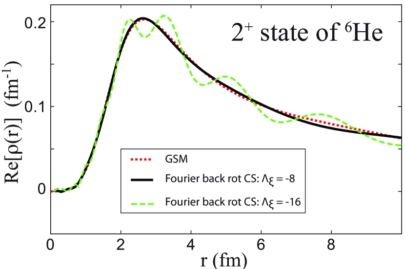
Figure 11: (Color online) Real part of one-neutron radial density for the 2⁺ resonance in ⁶He obtained in back-rotated CS-Slater using the Fourier-regularized analytical continuation with $\Lambda_{\xi}=-8$ (solid line) and $\Lambda_{\xi}=-16$ (dashed line). The GSM density is marked by a dotted line.

By taking the cutoff parameter $\Lambda_{\xi}=-8$ we obtain a density that is almost identical to that of the GSM. With $\Lambda_{\xi}=-16$, the analytically-continued density starts to oscillate around the GSM result, and with even larger negative values of cutoff used, the high-frequency components become amplified and eventually one recoups the highly-fluctuating direct back-rotation result of Fig. 9.

In the Tikhonov method, the sharp cutoff $\Lambda_{\xi}$ is replaced by a smooth cutoff (or filter) characterized by a smoothing parameter $\kappa$. In Eq. (46) this has been achieved by means of the damping function (regulator) $[1+\kappa\exp(-2y\xi)]^{-1}$ that attenuates large negative values of $\xi$, with the parameter $\kappa$ controlling the degree of regularization. The functional form of the regulator is not unique; it depends on the nature of the problem. In the applications presented in this study, the analytically-continued density coincides with the $\vartheta$-independent result for $\kappa$ = 4$\times$10^-4, which also corresponds to the original resonant GSM solution. The results presented in Figs. 9 and 10 demonstrate that both real and imaginary parts of the resonance’s density obtained in the Tikhonov-regularized CS-Slater method are in excellent agreement with the GSM result.

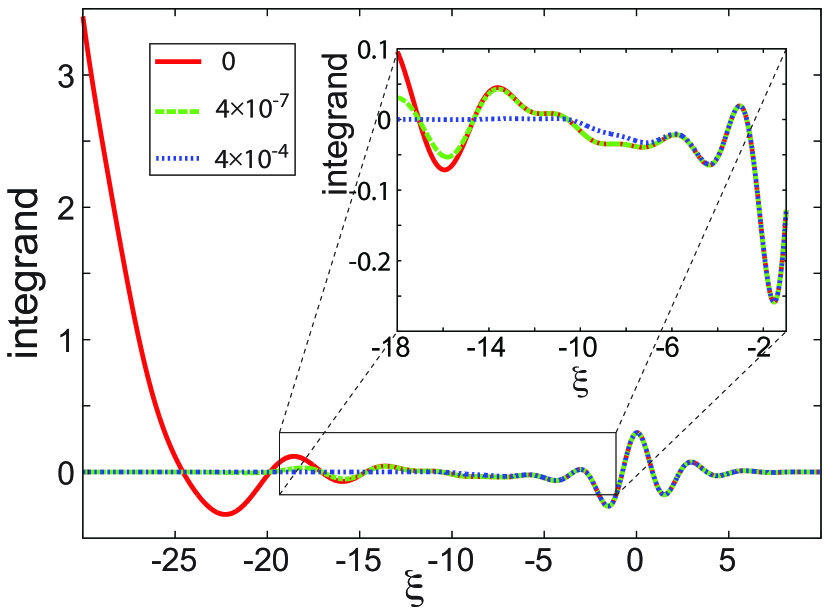
Figure 12: (Color online) The real part of the integrand in Eq. (46), calculated at $r=20$ fm, $\vartheta_{\rm opt}=0.43$, and $\kappa$=0, 4$\times$10^-7, and 4$\times$10^-4. To see the detailed behavior at small negative values of $\xi$, the region of $-18\leq$ $\xi$ $\leq-1$ is shown in the inset.

To understand in more detail the mechanism behind the Tikhonov regularization, in Fig.12 we display the real part of the integrand in (45) at $r=20$ fm, $\vartheta_{\rm opt}=0.43$, and $\kappa=0$ (no regularization), $\kappa=4\times$$10^{-7}$ and 4$\times$10^-4. In the absence of regulator, at $\xi<-10$ the integrand exhibits oscillations with increasing amplitude. Below $\xi=-8$, all three variants of calculations are very close; this explains the excellent agreement between GSM and back-rotated CS result in Fig. 11 with $\Lambda_{\xi}=-8$. In short, with the Tikhonov method, large values of the integrand at large negative values of $\xi$ are suppressed, thus enabling us to obtain an excellent reproduction of the resonant density in GSM.

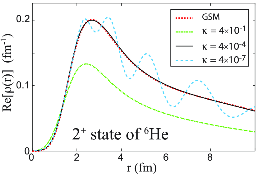
Figure 13: (Color online) Real part of one-neutron radial density for the 2⁺ resonance in ⁶He obtained in back-rotated CS-Slater method using the Tikhonov regularization with several values of smoothing parameter $\kappa$.

It is instructive to study the behavior of the analytically continued back-rotated CS density for different Tikhonov regularization parameters $\kappa$. As mentioned earlier, the value $\kappa$ = 4$\times$10^-4 was found to be optimal, i.e., it produces the CS-Slater densities that are closest to those of GSM. As seen in Fig. 13, for smaller values of $\kappa$, the damping function is too small to eliminate the oscillations at large negative $\xi$ values. This is also depicted in Fig. 12, where for $\kappa$ = 4$\times$10^-7 unwanted oscillations of the integrand appear around $\xi\sim 16$. For larger values of $\kappa$, the integral is over-regulated and produces a suppressed density profile. Similar patterns of $\kappa$-dependence have been found in other studies Hansen (1992); O’Leary (2001); Golub et al. (1979, 1999).

Figure 14: (Color online) Real (a) and imaginary (b) parts of one-neutron radial density at $r=3$ and 6  fm for the $2^{+}$ resonance in ⁶He, as a function of the Tikhonov regularization parameter $\kappa$. In an intermediate region of $\kappa$ values (grey shading), plateaus appear that coincide with the GSM results.

The behavior seen in Fig. 13 suggests a way to determine the optimal value of the smoothing parameter $\kappa$, regardless of the availability of the GSM result. The idea behind our method is presented in Fig. 14 that shows the values of $\rho(r)$ at two chosen large distances $r_{\kappa}$ (here $r_{\kappa}=3$ and 6 fm) versus $\kappa$ in a fairly broad range. As expected, at large and small values of $\kappa$, $\rho(r_{\kappa})$ shows strong variations with the Tikhonov smoothing parameter. However, at intermediate values, plateau in $\rho(r_{\kappa})$ appears that nicely coincides with the GSM results. Our optimal choice, $\kappa_{\rm opt}=4\times 10^{-4}$, belongs to this plateau.

IV.3 Two-body angular densities

The two-body density contains information about two-neutron correlations. It is defined as Viollier and Walecka (1977); *cor_def2; *cor_def3:

$$\rho(\bm{r},\bm{r^{\prime}})=\langle\Psi|\delta(\bm{r}-\bm{r}_{1})\delta(\bm{r^{\prime}}-\bm{r}_{2})|\Psi\rangle.$$ (48)

In spherical coordinates, it is convenient to introduce Papadimitriou et al. (2011)

$$\rho(r,r^{\prime},\theta)=\langle\Psi|\delta(r_{1}-r)\delta(r_{2}-r^{\prime})\delta(\theta_{12}-\theta)|\Psi\rangle,$$ (49)

with $r_{1}$ ($r_{2}$) being the distance between the core and the first (second) neutron and $\theta_{12}$ - the opening angle between the two neutrons. The density $\rho(r,r^{\prime},\theta)$ differs from the two-particle density (48) by the absence of the Jacobian $8\pi^{2}r^{2}r^{\prime 2}\sin\theta$. Consequently, the two-body density is normalized according to

$$\int\rho(r,r^{\prime},\theta)drdr^{\prime}d\theta=1.$$ (50)

In practical applications, (49) is calculated and plotted for $r=r^{\prime}$.

By parametrizing the wave function in terms of the distance $r$ from the core nucleus and the angle $\theta$ between the valence particles, one is able to investigate the particle correlations in the halo nucleus. Such calculations were performed recently Papadimitriou et al. (2011) to explain the observed charge radii differences in helium halo nuclei Lu et al. (2013).

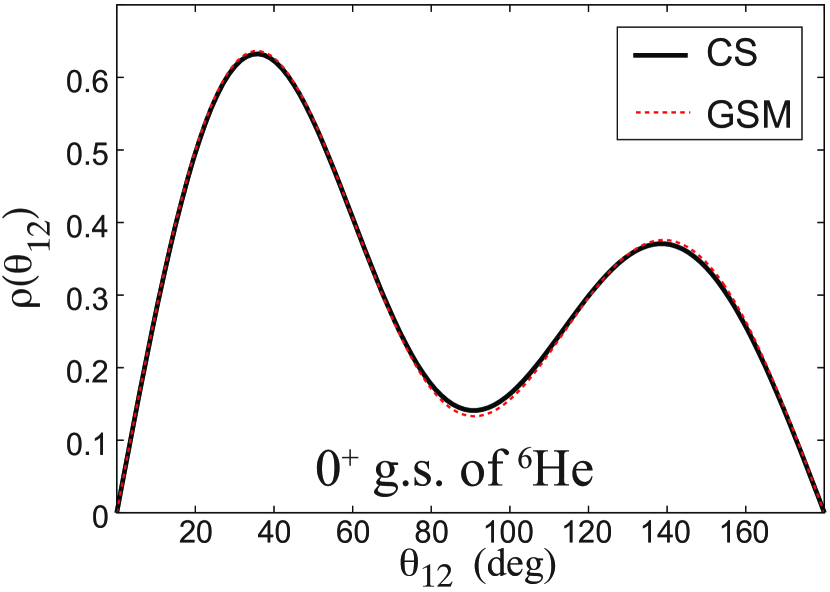
Figure 15: (Color online) Angular two-neutron density for the ⁶He g.s. predicted in GSM and CS-Slater.

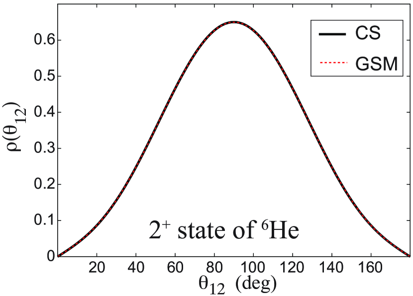
Figure 16: (Color online) Similar as in Fig.15 but for the 2⁺ resonance.

To study angular correlations between valence particles, we introduce the angular density:

$$\rho(\theta_{12})=\int\,dr\int\,dr^{\prime}\rho(r,r^{\prime},\theta_{12}).$$ (51)

Figures 15 and 16 display $\rho(\theta_{12})$ for the g.s. and $2^{+}_{1}$ resonance, respectively. The agreement between GSM and CS-Slater is excellent. It is worth noting that the calculation of the angular density in the CS-Slater framework does not require back-rotation. Indeed, since the CS operator (5) acts only on the radial coordinates, once they are integrated out one obtains the unscaled result.

V Conclusions

In this work, we introduce the new efficient CS method in a Slater basis to treat open many-body systems. We apply the new technique to the two-neutron halo nucleus ⁶He considered as a three body problem. The interaction between valence neutrons is modelled by a finite-range Minnesota force.

To benchmark the new method, we computed the weakly bound g.s. and $2^{+}_{1}$ resonance in ⁶He in both CS-Slater and GSM. We carefully studied the numerical accuracy of both methods and found it more than sufficient for the purpose of benchmarking. Based on our tests, we find both approaches equivalent for all the quantities studied. In a parallel development Masui et al. (2008, 2013), the CS method in a Gaussian basis Hiyama et al. (2003) has been compared with GSM for ⁶He and ⁶Be and a good overall agreement has been found.

An important aspect of our study was the application of the Tikhonov regularization technique to CS-Slater back-rotated wave functions in order to minimize the ultraviolet numerical noise at finite scaling angles $\vartheta$. We traced back the origin of high-frequency oscillations to the high-frequency part of the Fourier transform associated with the analytic continuation of the CS wave function and found the practical way to determine the smoothing parameter defining the Tikhonov regularization. The applied stabilization method allows to reconstruct the correct radial asymptotic behavior by using localized complex-scaled wave functions. This can be of importance when calculating observables that are directly related to the asymptotic behavior of the system, such as cross sections or decay widths. The proposed method is valid not only for narrow resonances (as for example Ref. Lefebvre (1992)), but also for broad resonant states, such as the excited 2⁺ state of ⁶He.

In the near future, we intend to include the inter-nucleon distance $r_{12}$ in Eq. (12) to obtain the full Hylleraas basis that promises somehow improved numerical convergence and higher accuracy. This will enable us to formulate the reaction theory directly in Hylleraas coordinates. The near-term application could include the $\alpha+d$ elastic scattering and the radiative capture reactions as in Kikuchi et al. (2011), and atomic applications such as electron-hydrogen scattering.

*

Appendix A Radial integrals

To simplify the radial integral (II.2.2) we use the explicit form of the Legendre polynomial $P_{\lambda}(x)=\sum_{n=0}^{\lambda}\eta_{\lambda,n}x^{n}$ and the binomial theorem to get:

$$I^{(\lambda)}(n_{13},n_{23})=\sum_{n=0}^{\lambda}{\eta_{\lambda,n}}{2^{-n}}\sum_{k=0}^{n}{{n}\choose{k}}\sum_{m=0}^{k}(-1)^{k}{{k}\choose{m}}$$

$$\times\int_{0}^{\infty}dr_{13}\,r_{13}^{n_{13}+n-2k+1}e^{-a_{13}r_{13}}\int_{0}^{\infty}dr_{23}\,r_{23}^{n_{23}+2k-2m-n+1}e^{-a_{23}r_{23}}\int_{|r_{13}-r_{23}|}^{r_{13}+r_{23}}dr_{12}\ r_{12}^{2m+1}V_{12}(r_{12}).$$ (52)

Now we make a variable transformation from the relative coordinates $r_{12},r_{13}$ and $r_{23}$ to the Hylleraas coordinates $s,t,u$ defined by the equations $s=r_{13}+r_{23}$, $t=r_{13}-r_{23}$, and $u=r_{12}$. Expressed in $s,t$, and $u$, the radial volume element becomes $d\tau_{r}=\frac{1}{8}(s^{2}-t^{2})ds\,du\,dt$, and (A) can be written as:

$$I^{(\lambda)}(n_{13},n_{23})=\sum_{n=0}^{\lambda}\eta_{\lambda,n}{2^{-n}}\sum_{k=0}^{n}{{n}\choose{k}}\sum_{m=0}^{k}(-1)^{k}{{k}\choose{m}}\sum_{k_{13}=0}^{N_{13}+1}\sum_{k_{23}=0}^{N_{23}+1}2^{-3-N_{13}-N_{23}}$$

$$\times{{N_{13}+1}\choose{k_{13}}}{{N_{23}+1}\choose{k_{23}}}(-1)^{k_{23}}\int_{0}^{\infty}ds\,e^{-as}s^{N_{13}+N_{23}+2-k_{13}-k_{23}}\int_{0}^{s}du\,u^{N_{12}}V_{12}(u)\int_{0}^{u}dt\,t^{k_{13}+k_{23}}e^{-bt},$$ (53)

where $a=\frac{1}{2}(a_{13}+a_{23})$, $b=\frac{1}{2}(a_{13}-a_{23})$, $N_{12}=2m+1$, $N_{13}=n_{13}+n-2k$, and $N_{23}=n_{23}+2k-2m-n$. With the help of the integral

$$I(n_{s},n_{t},n_{u},a,b)=\int_{0}^{\infty}ds\,s^{n_{s}}e^{-as}\int_{0}^{s}du\,u^{n_{u}}V_{12}(u)\int_{0}^{u}dt\,t^{n_{t}}e^{-bt}$$ (54)

we can write:

$$I^{(\lambda)}(n_{13},n_{23})=\sum_{n=0}^{\lambda}{\eta_{\lambda,n}}{2^{-n}}\sum_{k=0}^{n}{{n}\choose{k}}\sum_{m=0}^{k}(-1)^{k}{{k}\choose{m}}\sum_{k_{13}=0}^{N_{13}+1}\sum_{k_{23}=0}^{N_{23}+1}{{N_{13}+1}\choose{k_{13}}}{{N_{23}+1}\choose{k_{23}}}$$

$$\times{(-1)^{k_{23}}}{2^{-3-N_{13}-N_{23}}}I(N_{13}+N_{23}+2-k_{13}-k_{23},k_{13}+k_{23},N_{12},a,b).$$ (55)

As the integral over $t$ in (54) can be carried out analytically and the integral over $u$ can be computed by using

$$\frac{d}{ds}\left(-\frac{1}{a^{n_{s}+1}}\Gamma(n_{s}+1,as)\right)=e^{-as}s^{n_{s}},$$ (56)

one gets:

$$I(n_{s},n_{t},n_{u},a,b)=\frac{1}{(n_{t}+1)a^{n_{s}+1}}\int_{0}^{\infty}ds\Gamma(n_{s}+1,as)$$

$$\times s^{n_{u}+n_{t}+1}V_{12}(s){\rm M}(n_{t}+1,n_{t}+2,-bs),$$ (57)

where ${\rm M}(n_{t}+1,n_{t}+2,-bs)$ is the regular confluent hypergeometric function and $\Gamma(n_{s}+1,as)$ is the incomplete Gamma function Abramowitz and Stegun (1965). Expressing these two special functions as finite sums of elementery functions one finally arrives at the compact general expression

$$I(n_{s},n_{t},n_{u},a,b)=\frac{n_{s}!n_{t}!}{a^{n_{s}+1}b^{n_{t}+1}}\times$$ (58)

$$\sum_{k=0}^{n_{s}}\frac{a^{k}}{k!}\int_{0}^{\infty}ds\,e^{-as}s^{n_{u}+k}V(s)\left[1-e^{-bs}\sum_{n=0}^{n_{t}}\frac{(bs)^{n}}{n!}\right],$$

which is valid for any form factor $V(r)$. It is immediately seen that for $b=0$ (58) simplifies to

$$I(n_{s},n_{t},n_{u},a,0)=\frac{n_{s}!}{a^{n_{s}+1}(n_{t}+1)}\sum_{k=0}^{n_{s}}\frac{a^{k}}{k!}$$

$$\times\int_{0}^{\infty}dse^{-as}V(s)s^{n_{u}+n_{t}+k+1}.$$ (59)

To compute (58) with a Gaussian form factor $V(s)=\exp(-fs^{2})$, we use

$$\int_{0}^{\infty}ds\exp(-as-fs^{2})s^{n}=(-1)^{n}K^{(n)}(a),$$ (60)

where $K^{(n)}(z)=\frac{d^{n}}{dz^{n}}K(z)$ with

$$K(z)=\frac{1}{2}\sqrt{\frac{\pi}{f}}\exp\left(\frac{z^{2}}{4f}\right){\rm Erfc}\left(\frac{z}{2\sqrt{f}}\right).$$ (61)

Expressed in terms of the parabolic cylinder function $D_{-n-1}(z)$ Segura and Gil (1998), $K^{(n)}(z)$ is:

$$K^{(n)}(z)=\frac{1}{2}\sqrt{\frac{\pi}{f}}\left(\frac{1}{2\sqrt{f}}\right)^{n}\frac{(-1)^{n}n!2^{(n+1)/2}}{\sqrt{\pi}}$$

$$\exp(z^{2}/(8f))D_{-n-1}(z/\sqrt{2f}).$$ (62)