Analysis of interior penalty discontinuous Galerkin methods for the Allen-Cahn equation and the mean curvature flow

Abstract

This paper develops and analyzes two fully discrete interior penalty discontinuous Galerkin (IP-DG) methods for the Allen-Cahn equation, which is a nonlinear singular perturbation of the heat equation and originally arises from phase transition of binary alloys in materials science, and its sharp interface limit (the mean curvature flow) as the perturbation parameter tends to zero. Both fully implicit and energy-splitting time-stepping schemes are proposed. The primary goal of the paper is to derive sharp error bounds which depend on the reciprocal of the perturbation parameter $\epsilon$ (also called “interaction length”) only in some lower polynomial order, instead of exponential order, for the proposed IP-DG methods. The derivation is based on a refinement of the nonstandard error analysis technique first introduced in [12]. The centerpiece of this new technique is to establish a spectrum estimate result in totally discontinuous DG finite element spaces with a help of a similar spectrum estimate result in the conforming finite element spaces which was established in [12]. As a nontrivial application of the sharp error estimates, they are used to establish convergence and the rates of convergence of the zero-level sets of the fully discrete IP-DG solutions to the classical and generalized mean curvature flow. Numerical experiment results are also presented to gauge the theoretical results and the performance of the proposed fully discrete IP-DG methods.

1 Introduction

The singular perturbation of the heat equation to be considered in this paper has the form

(1) $$u_{t}-\Delta u+\frac{1}{\epsilon^{2}}f(u)=0\qquad\mbox{in }\Omega_{T}:=\Omega\times(0,T),$$

where $\Omega\subseteq\mathbf{R}^{d}\,(d=2,3)$ is a bounded domain and $f=F^{\prime}$ for some double well potential density function $F$. In this paper we focus on the following widely used quartic density function:

(2) $$F(u)=\frac{1}{4}(u^{2}-1)^{2}.$$

Equation (1), which is known as the Allen-Cahn equation in the literature, was originally introduced by Allen and Cahn in [2] as a model to describe the phase separation process of a binary alloy at a fixed temperature. In the equation $u$ denotes the concentration of one of the two species of the alloy, and $\epsilon$ represents the interaction length. We remark that equation (1) differs from the original Allen-Cahn equation in the scaling of the time, $t$ here represents $\frac{t}{\epsilon^{2}}$ in the original formulation, hence, it is a fast time. To completely describe the physical (and mathematical) problem, equation (1) must be complemented with appropriate initial and boundary conditions. The following boundary and initial conditions will be considered in this paper:

(3) $$\frac{\partial u}{\partial n} =0 \qquad\mbox{in }\partial\Omega_{T}:=\partial\Omega\times(0,T),$$

(4) $$u =u_{0} \qquad\mbox{in }\Omega\times\{t=0\}.$$

In addition to the important role it plays in materials phase transition, the Allen-Cahn equation has also been well-known and intensively studied in the past thirty years due to its connection to the celebrated curvature driven geometric flow known as the mean curvature flow  or the motion by mean curvature (cf. [10, 14] and the references therein). It was proved that [10] the zero-level set $\Gamma_{t}^{\epsilon}:=\{x\in\Omega;u(x,t)=0\}$ of the solution $u$ to the problem (1)–(4) converges to the mean curvature flow which refers to the evolution of a curve/surface governed by the geometric law $V_{n}=\kappa$, where $V_{n}$ and $\kappa$ respectively stand for the (inward) normal velocity and the mean curvature of the curve/surface. In fact, the Allen-Cahn equation (and the related Cahn-Hilliard equation) has emerged as a fundamental equation as well as a building block in the phase field methodology or the diffuse interface methodology for moving interface and free boundary problems arising from various applications such as fluid dynamics, materials science, image processing and biology (cf [11, 17] and the references therein). The diffuse interface method provides a convenient mathematical formalism for numerically approximating the moving interface problems because there is no need to explicitly compute the interface in the diffuse interface formulation. The biggest advantage of the diffuse interface method is its ability to handle with ease singularities of the interfaces. Computationally, like many singular perturbation problems, the main issue is to resolve the (small) scale introduced by the parameter $\epsilon$ in the equation. The problem could become intractable, especially in three-dimensional case if uniform meshes are used. This difficulty is often overcome by exploiting the predictable (at least for small $\epsilon$) PDE solution profile and by using adaptive mesh techniques (cf. [16, 13]) so fine meshes are only used in a small neighborhood of the phase front.

Numerical approximations of the Allen-Cahn equation have been extensively investigated in the past thirty years (cf. [3, 8, 12] and the references therein). However, most of these works were carried out for a fixed parameter $\epsilon$. The error estimates, which are obtained using the standard Gronwall inequality technique, show an exponential dependence on $\frac{1}{\epsilon}$. Such an estimate is clearly not useful for small $\epsilon$, in particular, in addressing the issue whether the flow of the computed numerical interfaces converge to the original sharp interface model: the mean curvature flow. Better error estimates should only depend on $\frac{1}{\epsilon}$ in some (low) polynomial orders because they can be used to provide an answer to the above convergence issue. In fact, such an estimate is the best result (in terms of $\epsilon$) one can expect. The first such polynomial order in $\frac{1}{\epsilon}$ a priori estimate was obtained by Feng and Prohl in [12] for standard finite element approximations of the Allen-Cahn problem (1)–(4). Extensions of the results of [12], in particular, the sensitivity of the eigenvalue to the topology was later considered, and some numerical tests were also given by Bartels et al. in [3]. In addition, polynomial order in $\frac{1}{\epsilon}$ a posteriori error estimates were obtained in [16, 13, 3]. One of the key ideas employed in all these works is to use a nonstandard error estimate technique which is based on establishing a discrete spectrum estimate (using its continuous counterpart) for the linearized Allen-Cahn operator. An immediate application of the polynomial order in $\frac{1}{\epsilon}$ a priori and a posteriori error estimates is to prove the convergence of the numerical interfaces of the underlying finite element approximations to the mean curvature flow as $\epsilon$ and mesh sizes $h$ and $\tau$ all tend to zero, and to establish rates of convergence (in powers of $\epsilon$) for the numerical interfaces before the onset of singularities of the mean curvature flow.

The primary objectives of this paper are twofold: First, we want to develop some interior penalty discontinuous Galerkin (IP-DG) methods and to establish polynomial order in $\frac{1}{\epsilon}$ a priori error estimates as well as to prove convergence and rates of convergence for the IP-DG numerical interfaces. This goal is motivated by the advantages of DG methods in regard to designing adaptive mesh methods and algorithms, which is an indispensable strategy with the diffuse interface methodology. Second, we use the Allen-Cahn equation as a prototype to develop new analysis techniques for analyzing convergence of numerical interfaces to the sharp interface for DG (and nonconforming finite element) discretizations of phase field models. To the best of our knowledge, no such convergence result and analysis technique is available in the literature. The main obstacle for adapting the techniques of [12] is that the DG (and nonconforming finite element) spaces are not subspaces of $H^{1}(\Omega)$. As a result, whether the desired discrete spectrum estimate holds becomes a key question to answer.

The remainder of this paper is organized as follows. In section 2 we first recall some facts about the Allen-Cahn equation. In particular, we cite the spectrum estimate for the linearized Allen-Cahn operator from [6] and a nonlinear discrete Gronwall inequality from [19]. In section 3 we present two fully nonlinear IP-DG methods for problem (1)–(4) with the implicit Euler time stepping for the linear terms. The two methods differ in how the nonlinear term is discretized in time. The first is fully implicit and the second uses a well-known energy splitting idea due to Ere [9]. The rest of section 3 devotes to the convergence analysis of the proposed IP-DG methods. The highlights of analysis include establishing a discrete spectrum estimate for the linearized Allen-Cahn operator in DG spaces and deriving optimal order (in $h$ and $\tau$) and polynomial order in $\frac{1}{\epsilon}$ a priori error estimates for the proposed IP-DG methods. In section 4, using the error estimates of section 3 we prove the convergence and rates of convergence for the numerical interfaces of the IP-DG solutions to the sharp interface of the mean curvature flow. Finally, we present some numerical experiment results in section 5 to gauge the performance of the proposed fully discrete IP-DG methods.

2 Preliminaries

In this section, we first recall a few facts about the solution of the problem (1)–(4) which can be found in [12, 6]. These facts will be used in the analysis of section 3 and 4. We then cite a lemma which provides an upper bound for discrete sequences that satisfy a Bernoulli-type inequality, and this lemma is crucially used in our error analysis in section 3. Standard function and space notations are adopted in this paper. $(\cdot,\cdot)_{\Omega}$ denotes the standard inner product on $L^{2}(\Omega)$, $C$ and $c$ denote generic positive constants which is independent of $\epsilon$, space and time step sizes $h$ and $\tau$. We begin by recalling a well-known fact [10, 14] that the Allen-Cahn equation (1) can be interpreted as the $L^{2}$-gradient flow for the following Cahn-Hilliard energy functional

(5) $$J_{\epsilon}(v):=\int_{\Omega}\Bigl{(}\frac{1}{2}|\nabla v|^{2}+\frac{1}{\epsilon^{2}}F(v)\Bigr{)}\,dx$$

In order to derive a priori solution estimates, as in [12] we make the following assumptions on the initial datum $u_{0}$.

General Assumption (GA)

• There exists a nonnegative constant $\sigma_{1}$ such that

  (6) $$J_{\epsilon}(u_{0})\leq C\epsilon^{-2\sigma_{1}}.$$

• There exists a nonnegative constant $\sigma_{2}$ such that

  (7) $$\|\Delta u_{0}-\epsilon^{-2}f(u_{0})\|_{L^{2}(\Omega)}\leq C\epsilon^{-\sigma_{2}}.$$

• There exists nonnegative constant $\sigma_{3}$ such that

  (8) $$\lim_{s\rightarrow 0^{+}}\|\nabla u_{t}(s)\|_{L^{2}(\Omega)}\leq C\epsilon^{-\sigma_{3}}.$$

The following solution estimates can be found in [12].

Proposition 1.

Suppose that (6) and (7) hold. Then the solution $u$ of problem (1)–(4) satisfies the following estimates:

(9) $$\underset{t\in[0,\infty)}{\mbox{\rm ess sup }}\|u(t)\|_{L^{\infty}(\Omega)}\leq\|u_{0}\|_{L^{\infty}(\Omega)},$$

(10) $$\underset{t\in[0,\infty)}{\mbox{\rm ess sup }}\,J_{\epsilon}(u)+\int_{0}^{\infty}\|u_{t}(s)\|_{L^{2}(\Omega)}^{2}\,ds\leq C\epsilon^{-2\sigma_{1}},$$

(11) $$\int_{0}^{T}\|\Delta u(s)\|^{2}\,ds\leq C\epsilon^{-2(\sigma_{1}+1)},$$

(12) $$\underset{t\in[0,\infty)}{\mbox{\rm ess sup }}\Bigl{(}\|u_{t}\|_{L^{2}(\Omega)}^{2}+\|u\|_{H^{2}(\Omega)}^{2}\Bigr{)}+\int_{0}^{\infty}\|\nabla u_{t}(s)\|_{L^{2}(\Omega)}^{2}\,ds\leq C\epsilon^{-2\max\{\sigma_{1}+1,\sigma_{2}\}},$$

(13) $$\int_{0}^{\infty}\Bigl{(}\|u_{tt}(s)\|_{H^{-1}(\Omega)}^{2}+\|\Delta u_{t}(s)\|_{H^{-1}(\Omega)}^{2}\Bigr{)}\,ds\leq C\epsilon^{-2\max\{\sigma_{1}+1,\sigma_{2}\}}.$$

In addition to (6) and (7), suppose that (8) holds, then $u$ also satisfies

(14) $$\underset{t\in[0,\infty)}{\mbox{\rm ess sup }}\|\nabla u_{t}\|_{L^{2}(\Omega)}^{2}+\int_{0}^{\infty}\|u_{tt}(s)\|_{L^{2}}^{2}\,ds\leq C\epsilon^{-2\max\{\sigma_{1}+2,\sigma_{3}\}},$$

(15) $$\int_{0}^{\infty}\|\Delta u_{t}(s)\|_{L^{2}(\Omega)}^{2}\,ds\leq C\epsilon^{-2\max\{\sigma_{1}+2,\sigma_{3}\}}.$$

Next, we quote a lower bound estimate for the principal eigenvalue of the following linearized Allen-Cahn operator:

(16) $$\mathcal{L}_{\mbox{\tiny AC}}:=-\Delta+f^{\prime}(u)I,$$

where $I$ stands for the identity operator.

Proposition 2.

Suppose that (6) and (7) hold, and $u_{0}$ satisfies some profile as described in [6]. Let $u$ denote the solution of problem (1)–(4). Then there exists a positive $\epsilon$-independent constant $C_{0}$ such that the principle eigenvalue of the linearized Allen-Cahn operator ${\mathcal{L}}_{\mbox{\tiny AC}}$ satisfies for $0<\epsilon<<1$

(17) $$\lambda_{\mbox{\tiny AC}}\equiv\inf_{\psi\in H^{1}(\Omega)\atop\psi\neq 0}\frac{\|\nabla\psi\|_{L^{2}(\Omega)}^{2}+\epsilon^{-2}\,\bigl{(}f^{\prime}(u)\psi,\psi\bigr{)}}{\|\psi\|_{L^{2}(\Omega)}^{2}}\geq-C_{0}.$$

Remark 1.

(a) A proof of Proposition 2 can be found in [6]. A discrete generalization of (17) on $C^{0}$ finite element spaces was proved in [12]. It plays a pivotal role in the nonstandard convergence analysis of [12]. In the next section, we shall prove another discrete generalization of (17) on DG finite element spaces.

(b) The restriction on the initial function $u_{0}$ is needed to guarantee that the solution $u(t)$ satisfies certain profile at later time $t>0$ which is required in the proof of [6]. One example of admissible initial functions is $u_{0}=tanh(\frac{d_{0}(x)}{\epsilon})$, where $d_{0}(x)$ stands for the signed distance function to the initial interface $\Gamma_{0}$.

The classical Gronwall lemma derives an estimate for any function which satisfies a first order linear differential inequality. It is a main technique for deriving error estimates for continuous-in-time semi-discrete discretizations of many initial-boundary value PDE problems. Similarly, the discrete counterpart of Gronwall lemma is a main technical tool for deriving error estimates for fully discrete schemes. However, for many nonlinear PDE problems, the classical Gronwall lemma does not apply because of nonlinearity, instead, some nonlinear generalization must be used. In case of the power (or Bernoulli-type) nonlinearity, a generalized Gronwall lemma was proved in [13]. In the following we state a discrete counterpart of the lemma in [13], and the proof of a similar lemma can be found in [19]. This lemma will be utilized crucially in the next section.

Lemma 3.

Let $\{S_{\ell}\}_{\ell\geq 1}$ be a positive nondecreasing sequence and $\{b_{\ell}\}_{\ell\geq 1}$ and $\{k_{\ell}\}_{\ell\geq 1}$ be nonnegative sequences, and $p>1$ be a constant. If

(18) $$S_{\ell+1}-S_{\ell}\leq b_{\ell}S_{\ell}+k_{\ell}S^{p}_{\ell}\qquad\mbox{for }\ell\geq 1,$$

(19) $$S^{1-p}_{1}+(1-p)\mathop{\sum}\limits_{s=1}^{\ell-1}k_{s}a^{1-p}_{s+1}>0\qquad\mbox{for }\ell\geq 2,$$

then

(20) $$S_{\ell}\leq\frac{1}{a_{\ell}}\Bigg{\{}S^{1-p}_{1}+(1-p)\sum_{s=1}^{\ell-1}k_{s}a^{1-p}_{s+1}\Bigg{\}}^{\frac{1}{1-p}}\qquad\text{for}\ \ell\geq 2,$$

where

(21) $$a_{\ell}:=\prod_{s=1}^{\ell-1}\frac{1}{1+b_{s}}\qquad\mbox{for }\ell\geq 2.$$

3 Fully discrete IP-DG approximations

3.1 Formulations

Let $\mathcal{T}_{h}$ be a quasi-uniform “triangulation” of $\Omega$ such that $\overline{\Omega}=\bigcup_{K\in\mathcal{T}_{h}}\overline{K}$. Let $h_{K}$ denote the diameter of $K\in\mathcal{T}_{h}$ and $h:=\mbox{max}\{h_{K};K\in\mathcal{T}_{h}\}$. We recall that the standard broken Sobolev space $H^{s}(\mathcal{T}_{h})$ and DG finite element space $V_{h}$ are defined as

$$H^{s}(\mathcal{T}_{h}):=\prod_{K\in\mathcal{T}_{h}}H^{s}(K),\qquad V_{h}:=\prod_{K\in\mathcal{T}_{h}}P_{r}(K),$$

where $P_{r}(K)$ denotes the set of all polynomials whose degrees do not exceed a given positive integer $r$. Let $\mathcal{E}_{h}^{I}$ denote the set of all interior faces/edges of $\mathcal{T}_{h}$, $\mathcal{E}_{h}^{B}$ denote the set of all boundary faces/edges of $\mathcal{T}_{h}$, and $\mathcal{E}_{h}:=\mathcal{E}_{h}^{I}\cup\mathcal{E}_{h}^{B}$. The $L^{2}$-inner product for piecewise functions over the mesh $\mathcal{T}_{h}$ is naturally defined by

$$(v,w)_{\mathcal{T}_{h}}:=\sum_{K\in\mathcal{T}_{h}}\int_{K}vw\,dx,$$

and for any set $\mathcal{S}_{h}\subset\mathcal{E}_{h}$, the $L^{2}$-inner product over $\mathcal{S}_{h}$ is defined by

$$\big{\langle}v,w\big{\rangle}_{\mathcal{S}_{h}}:=\sum_{e\in\mathcal{S}_{h}}\int_{e}vw\,ds.$$

Let $K,K^{\prime}\in\mathcal{T}_{h}$ and $e=\partial K\cap\partial K^{\prime}$ and assume global labeling number of $K$ is smaller than that of $K^{\prime}$. We choose $n_{e}:=n_{K}|_{e}=-n_{K^{\prime}}|_{e}$ as the unit normal on $e$ and define the following standard jump and average notations across the face/edge $e$:

$$[v] :=v|_{K}-v|_{K^{\prime}}\quad \mbox{on }e\in\mathcal{E}_{h}^{I},\qquad [v]:=v\quad \mbox{on }e\in\mathcal{E}_{h}^{B},$$

$$\{v\} :=\frac{1}{2}\bigl{(}v|_{K}+v|_{K^{\prime}}\bigr{)}\quad \mbox{on }e\in\mathcal{E}_{h}^{I},\qquad \{v\}:=v\quad \mbox{on }e\in\mathcal{E}_{h}^{B}$$

for $v\in V_{h}$.

Let $M$ be a (large) positive integer. Define $\tau:=T/M$ and $t_{m}:=m\tau$ for $m=0,1,2,\cdots,M$ be a uniform partition of $[0,T]$. For a sequence of functions $\{v^{m}\}_{m=0}^{M}$, we define the (backward) difference operator

$$d_{t}v^{m}:=\frac{v^{m}-v^{m-1}}{k},\qquad m=1,2,\cdots,M.$$

We are now ready to introduce our fully discrete DG finite element methods for problem (1)–(4). They are defined by seeking $u_{h}^{m}\in V_{h}$ for $m=0,1,2,\cdots,M$ such that

(22) $$\bigl{(}d_{t}u_{h}^{m+1},v_{h}\bigr{)}_{\mathcal{T}_{h}}+a_{h}(u_{h}^{m+1},v_{h})+\frac{1}{\epsilon^{2}}\bigl{(}f^{m+1},v_{h}\bigr{)}_{\mathcal{T}_{h}} =0 \quad\forall v_{h}\in V_{h},$$

where

(23) $$a_{h}(w_{h},v_{h}) :=\bigl{(}\nabla w_{h},\nabla v_{h}\bigr{)}_{\mathcal{T}_{h}}-\bigl{\langle}\{\partial_{n}w_{h}\},[v_{h}]\bigr{\rangle}_{\mathcal{E}_{h}^{I}}$$

$$\hskip 79.49744pt+\lambda\bigl{\langle}[w_{h}],\{\partial_{n}v_{h}\}\bigr{\rangle}_{\mathcal{E}_{h}^{I}}+j_{h}(w_{h},v_{h}),$$

(24) $$j_{h}(w_{h},v_{h}) :=\sum_{e\in\mathcal{E}_{h}^{I}}\frac{\sigma_{e}}{h_{e}}\big{\langle}[w_{h}],[v_{h}]\big{\rangle}_{e},$$

(25) $$f^{m+1} :=(u_{h}^{m+1})^{3}-u_{h}^{m}\quad\mbox{or}\quad f^{m+1}:=(u_{h}^{m+1})^{3}-u_{h}^{m+1},$$

where $\lambda=0,\pm 1$ and $\sigma_{e}$ is a positive piecewise constant function on $\mathcal{E}_{h}^{I}$, which will be chosen later (see Lemma 5). In addition, we need to supply $u_{h}^{0}$ to start the time-stepping, whose choice will be clear (and will be specified) later when we derive the error estimates in section 3.4.

We conclude this subsection with a few remarks to explain the above IP-DG methods.

Remark 2.

(a) The mesh-dependent bilinear form $a_{h}(\cdot,\cdot)$ is a well-known IP-DG discretization of the negative Laplace operator $-\Delta$, see [20].

(b) Different choices of $\lambda$ give different schemes. In this paper we only focus on the symmetric case with $\lambda=-1$. Also, $\sigma_{e}$ is called the penalty constant.

(c) The time discretization is the simple backward Euler method for the linear terms. However, we shall prove in section 3.2 that the treatment of the nonlinear term results in two implicit schemes which have different stability properties with respect to $\epsilon$. We also note that only fully implicit scheme (i.e., $f^{m+1}=(u_{h}^{m+1})^{3}-u_{h}^{m+1}$) was considered in [12], and the resulted finite element method was proved only conditionally stable there.

3.2 Discrete energy laws and well-posedness

As a gradient flow, problem (1)–(4) enjoys an energy law which leads to the estimate (10) and then the subsequent estimates given in Proposition 1. One simple criterion for building a numerical method for problem (1)–(4) is whether the method satisfies a discrete energy law which mimics the continuous energy law [12, 11]. The goal of this subsection is to show that the IP-DG methods proposed in the previous subsection are either unconditionally energy stable when $f^{m+1}=(u_{h}^{m+1})^{3}-u_{h}^{m}$ or conditionally energy stable when $f^{m+1}=(u_{h}^{m+1})^{3}-u_{h}^{m+1}$.

First, we introduce three mesh-dependent energy functionals which can be regarded as DG counterparts of the continuous Cahn-Hilliard energy $J_{\epsilon}$ defined in (5).

(26) $$\Phi^{h}(v) :=\frac{1}{2}\|\nabla v\|_{L^{2}(\mathcal{T}_{h})}^{2}-\bigl{\langle}\{\partial_{n}v\},[v]\bigr{\rangle}_{\mathcal{E}_{h}^{I}}+\frac{1}{2}j_{h}(v,v)\qquad\forall v\in H^{2}(\mathcal{T}_{h}),$$

(27) $$J_{\epsilon}^{h}(v) :=\Phi^{h}(v)+\frac{1}{\epsilon^{2}}\bigl{(}F(v),1\bigr{)}_{\mathcal{T}_{h}}\qquad\forall v\in H^{2}(\mathcal{T}_{h}),$$

(28) $$I_{\epsilon}^{h}(v) :=\Phi^{h}(v)+\frac{1}{\epsilon^{2}}\bigl{(}F_{c}^{+}(v),1\bigr{)}_{\mathcal{T}_{h}}\qquad\forall v\in H^{2}(\mathcal{T}_{h}),$$

where $F(v)=\frac{1}{4}(v^{2}-1)^{2}$ and $F_{c}^{+}(v):=\frac{1}{4}(v^{4}+1)$.

If we define $F_{c}^{-}(v):=\frac{1}{2}v^{2}$, then there holds the convex decomposition $F(v)=F_{c}^{+}(v)-F_{c}^{-}(v)$. It is easy to check that $\Phi^{h}$ and $I_{\epsilon}^{h}$ are convex functionals but $J_{\epsilon}^{h}$ is not because $F$ is not convex. Moreover, we have

Lemma 4.

Let $\lambda=-1$ in (23), then there holds for all $v_{h},w_{h}\in V_{h}$

(29) $$\Bigl{(}\frac{\delta\Phi^{h}(v_{h})}{\delta v_{h}},w_{h}\Bigr{)}_{\mathcal{T}_{h}} :=\lim_{s\to 0}\frac{\Phi^{h}(v_{h}+sw_{h})-\Phi^{h}(v_{h})}{s}=a_{h}(v_{h},w_{h}),$$

(30) $$\Bigl{(}\frac{\delta J_{\epsilon}^{h}(v_{h})}{\delta v_{h}},w_{h}\Bigr{)}_{\mathcal{T}_{h}}: =\lim_{s\to 0}\frac{J_{\epsilon}^{h}(v_{h}+sw_{h})-J_{\epsilon}^{h}(v_{h})}{s}$$

$$=a_{h}(v_{h},w_{h})+\frac{1}{\epsilon^{2}}\bigl{(}F^{\prime}(v_{h}),w_{h}\bigr{)}_{\mathcal{T}_{h}},$$

(31) $$\Bigl{(}\frac{\delta I_{\epsilon}^{h}(v_{h})}{\delta v_{h}},w_{h}\Bigr{)}_{\mathcal{T}_{h}}: =\lim_{s\to 0}\frac{I_{\epsilon}^{h}(v_{h}+sw_{h})-I_{\epsilon}^{h}(v_{h})}{s}$$

$$=a_{h}(v_{h},w_{h})+\frac{1}{\epsilon^{2}}\bigl{(}(F_{c}^{+})^{\prime}(v_{h}),w_{h}\bigr{)}_{\mathcal{T}_{h}}.$$

Since the proof is straightforward, we omit it to save space.

Remark 3.

We remark that (29)–(31) provide respectively the representations of the Fréchet derivatives of the energy functionals $\Phi^{h},J_{\epsilon}^{h}$ and $I_{\epsilon}^{h}$ in $V^{h}$. This simple observation is very helpful, it allows us to recast our DG formulations in (22)–(25) as a minimization/variation problem at each time step. It is also a deeper reason why the proposed DG methods satisfy some discrete energy laws to be proved below.

Lemma 5.

There exist constants $\sigma_{0},\alpha>0$ such that for $\sigma_{e}>\sigma_{0}$ for all $e\in\mathcal{E}_{h}$ there holds

(32) $$\Phi^{h}(v_{h})\geq\alpha\|v_{h}\|_{1,\mbox{\tiny DG}}^{2}\qquad\forall v_{h}\in V_{h},$$

where

(33) $$\|v_{h}\|_{1,\mbox{\tiny DG}}^{2}:=\|\nabla v_{h}\|_{L^{2}(\mathcal{T}_{h})}^{2}+j_{h}(v_{h},v_{h}).$$

Proof.

Inequality (32) follows immediately from the following observation

(34) $$2\Phi^{h}(v_{h})=a_{h}(v_{h},v_{h})\qquad\forall v_{h}\in V_{h},$$

and the well-known coercivity property of the DG bilinear form $a_{h}(\cdot,\cdot)$ (cf. [20]). ∎

We now are ready to state our discrete energy/stability estimates.

Theorem 6.

Let $\{u_{h}^{m}\}$ be a solution of scheme (22)–(25). Then there exists $\sigma_{0}^{\prime}>0$ such that for $\sigma_{e}>\sigma_{0}^{\prime},\forall e\in\mathcal{E}_{h}$

(35) $$J^{h}_{\epsilon}(u_{h}^{\ell})+k\sum_{m=0}^{\ell}R^{m}_{\epsilon,h}\leq J^{h}_{\epsilon}(u_{h}^{0})\qquad\mbox{for }0\leq\ell\leq M,$$

where

(36) $$R^{m}_{\epsilon,h} :=\Bigl{(}1\pm\frac{k}{2\epsilon^{2}}\Bigr{)}\|d_{t}u_{h}^{m+1}\|_{L^{2}(\mathcal{T}_{h})}^{2}+\frac{k}{4}\|\nabla d_{t}u_{h}^{m+1}\|_{L^{2}(\mathcal{T}_{h})}^{2}$$

$$\qquad+\frac{k}{4}j_{h}\bigl{(}d_{t}u_{h}^{m+1},d_{t}u_{h}^{m+1}\bigr{)}+\frac{k}{4\epsilon^{2}}\|d_{t}(|u_{h}^{m+1}|^{2}-1)\|_{L^{2}(\mathcal{T}_{h})}^{2},$$

and the “+” sign in the first term is taken when $f^{m+1}=(u_{h}^{m+1})^{3}-u_{h}^{m}$ and “-” sign is taken when $f^{m+1}=(u_{h}^{m+1})^{3}-u_{h}^{m+1}$.

Proof.

Setting $v=d_{t}u_{h}^{m+1}$ in (22) we get

(37) $$\|d_{t}u_{h}^{m+1}\|_{L^{2}(\mathcal{T}_{h})}^{2}+a_{h}(u_{h}^{m+1},d_{t}u_{h}^{m+1})+\frac{1}{\epsilon^{2}}\bigl{(}f^{m+1},d_{t}u_{h}^{m+1}\bigr{)}_{\mathcal{T}_{h}}=0.$$

By the algebraic identity $a(a-b)=\frac{1}{2}(a^{2}-b^{2})+\frac{1}{2}(a-b)^{2}$ we have

(38) $$a_{h}(u_{h}^{m+1},\nabla d_{t}u_{h}^{m+1})=\frac{1}{2}d_{t}a_{h}(u_{h}^{m+1},u_{h}^{m+1})+\frac{k}{2}\Bigl{(}\|\nabla d_{t}u_{h}^{m+1}\|_{L^{2}(\mathcal{T}_{h})}^{2}$$

$$\hskip 93.95122pt+2\bigl{\langle}\{d_{t}\partial_{n}u_{h}^{m+1}\},[d_{t}u_{h}^{m+1}]\bigr{\rangle}_{\mathcal{E}_{h}^{I}}+j_{h}\bigl{(}d_{t}u_{h}^{m+1},d_{t}u_{h}^{m+1}\bigr{)}\Bigl{)}.$$

It follows from the trace and Schwarz inequalities that

(39) $$2\bigl{\langle}\{d_{t}\partial_{n}u_{h}^{m+1}\},[d_{t}u_{h}^{m+1}]\bigr{\rangle}_{\mathcal{E}_{h}^{I}}\geq-2\|\{d_{t}\partial_{n}u_{h}^{m+1}\}\|_{L^{2}(\mathcal{E}_{h}^{I})}\|[d_{t}u_{h}^{m+1}]\|_{L^{2}(\mathcal{E}_{h}^{I})}$$

$$\hskip 115.63243pt\geq-Ch^{-\frac{1}{2}}\|d_{t}\nabla u_{h}^{m+1}\|_{L^{2}(\mathcal{T}_{h})}\|[d_{t}u_{h}^{m+1}]\|_{L^{2}(\mathcal{E}_{h}^{I})}$$

$$\hskip 115.63243pt\geq-\frac{1}{2}\|d_{t}\nabla u_{h}^{m+1}\|_{L^{2}(\mathcal{T}_{h})}^{2}-Ch^{-1}\|[d_{t}u_{h}^{m+1}]\|_{L^{2}(\mathcal{E}_{h}^{I})}^{2}.$$

Then there exists $\sigma_{1}>0$ such that for $\sigma_{e}>\sigma_{1}$

(40) $$a_{h}(u_{h}^{m+1},\nabla d_{t}u_{h}^{m+1}) \geq\frac{1}{2}d_{t}a_{h}(u_{h}^{m+1},u_{h}^{m+1})$$

$$\qquad+\frac{k}{4}\Bigl{(}\|\nabla d_{t}u_{h}^{m+1}\|_{L^{2}(\mathcal{T}_{h})}^{2}+j_{h}\bigl{(}d_{t}u_{h}^{m+1},d_{t}u_{h}^{m+1}\bigr{)}\Bigl{)}.$$

We now bound the third term on the left-hand side of (37) from below. We first consider the case $f^{m+1}=(u_{h}^{m+1})^{3}-u_{h}^{m}$. To the end, we write

$$f^{m+1} =u_{h}^{m+1}\bigl{(}|u_{h}^{m+1}|^{2}-1\bigr{)}+kd_{t}u_{h}^{m+1}$$

$$=\frac{1}{2}\bigl{(}(u_{h}^{m+1}+u_{h}^{m})+kd_{t}u_{h}^{m+1}\bigr{)}\bigl{(}|u_{h}^{m+1}|^{2}-1\bigr{)}+kd_{t}u_{h}^{m+1}.$$

A direct calculation then yields

(41) $$\frac{1}{\epsilon^{2}}\bigl{(}f^{m+1},d_{t}u_{h}^{m+1}\bigr{)}_{\mathcal{T}_{h}} \geq\frac{1}{4\epsilon^{2}}d_{t}\||u_{h}^{m+1}|^{2}-1\|_{L^{2}(\mathcal{T}_{h})}^{2}$$

$$\quad+\frac{k}{4\epsilon^{2}}\|d_{t}(|u_{h}^{m+1}|^{2}-1)\|_{L^{2}(\mathcal{T}_{h})}^{2}+\frac{k}{2\epsilon^{2}}\|d_{t}u_{h}^{m+1}\|_{L^{2}(\mathcal{T}_{h})}^{2}.$$

On the other hand, when $f^{m+1}=f(u_{h}^{m+1})=(u_{h}^{m+1})^{3}-u_{h}^{m+1}$, we have (cf. [12])

(42) $$\frac{1}{\epsilon^{2}}\bigl{(}f^{m+1},d_{t}u_{h}^{m+1}\bigr{)}_{\mathcal{T}_{h}} \geq\frac{1}{4\epsilon^{2}}d_{t}\||u_{h}^{m+1}|^{2}-1\|_{L^{2}(\mathcal{T}_{h})}^{2}$$

$$\quad+\frac{k}{4\epsilon^{2}}\|d_{t}(|u_{h}^{m+1}|^{2}-1)\|_{L^{2}(\mathcal{T}_{h})}^{2}-\frac{k}{2\epsilon^{2}}\|d_{t}u_{h}^{m+1}\|_{L^{2}(\mathcal{T}_{h})}^{2}.$$

It follows from (37), (40), (34) and (41) (resp. (42)) that

$$\Bigl{(}1\pm\frac{k}{2\epsilon^{2}}\Bigr{)}\|d_{t}u_{h}^{m+1}\|_{L^{2}(\mathcal{T}_{h})}^{2}+d_{t}\Bigl{(}\Phi^{h}(u_{h}^{m+1})+\frac{1}{4\epsilon^{2}}\||u_{h}^{m+1}|^{2}-1\|_{L^{2}(\mathcal{T}_{h})}^{2}\Bigr{)}$$

$$+\frac{k}{4}\Bigl{(}\|\nabla d_{t}u_{h}^{m+1}\|_{L^{2}(\mathcal{T}_{h})}^{2}+j_{h}\bigl{(}d_{t}u_{h}^{m+1},d_{t}u_{h}^{m+1}\bigr{)}+\frac{1}{\epsilon^{2}}\|d_{t}(|u_{h}^{m+1}|^{2}-1)\|_{L^{2}(\mathcal{T}_{h})}^{2}\Bigr{)}\leq 0.$$

Finally, applying the summation operator $k\sum_{m=0}^{M-1}$ and using the definition of $J_{\epsilon}^{h}$ we obtain the desired estimate (35). The proof is complete. ∎

The above theorem immediately infers the following corollary.

Corollary 7.

The scheme (22)–(25) is stable for all $h,k>0$ when $f^{m+1}=(u_{h}^{m+1})^{3}-u_{h}^{m}$ and is stable for $h>0,2\epsilon^{2}>k>0$ when $f^{m+1}=(u_{h}^{m+1})^{3}-u_{h}^{m+1}$, provided that $\sigma_{e}>\max\{\sigma_{0},\sigma_{0}^{\prime}\}$ for every $e\in\mathcal{E}_{h}$.

Theorem 8.

Suppose that $\sigma_{e}>\max\{\sigma_{0},\sigma_{1}\}$ for every $e\in\mathcal{E}_{h}$. Then there exists a unique solution $u_{h}^{m+1}$ to the scheme (22)–(25) at every time step $t_{m+1}$ for $h,k>0$ in the case $f^{m+1}=(u_{h}^{m+1})^{3}-u_{h}^{m}$. The conclusion still holds provided that $h>0,2\epsilon^{2}>k>0$ in the case $f^{m+1}=(u_{h}^{m+1})^{3}-u_{h}^{m+1}$.

Proof.

Define the following functionals

$$G(v) :=k\Phi^{h}(v)+\frac{k}{\epsilon^{2}}\bigl{(}F(v),1\bigr{)}_{\mathcal{T}_{h}}+\frac{1}{2}\|v\|_{L^{2}(\mathcal{T}_{h})}^{2}-\bigl{(}u_{h}^{m},v\bigr{)}_{\mathcal{T}_{h}},$$

$$H(v) :=k\Phi^{h}(v)+\frac{k}{\epsilon^{2}}\bigl{(}F_{c}^{+}(v),1\bigr{)}_{\mathcal{T}_{h}}+\frac{1}{2}\|v\|_{L^{2}(\mathcal{T}_{h})}^{2}-\Bigl{(}\frac{k}{\epsilon^{2}}+1\Bigr{)}\bigl{(}u_{h}^{m},v\bigr{)}_{\mathcal{T}_{h}}.$$

Clearly, $H$ is strictly convex for all $h,k>0$. $G$ is not always convex, however, it becomes strictly convex when $k<2\epsilon^{2}$. To see this, we write $F(v)=F_{c}^{+}(v)-F_{c}^{-}(v)$ in the definition of $G(v)$ and notice that

$$-\frac{k}{\epsilon^{2}}\bigl{(}F_{c}^{-}(v),1\bigr{)}_{\mathcal{T}_{h}}+\frac{1}{2}\|v\|_{L^{2}(\mathcal{T}_{h})}^{2}=\frac{1}{2}\Bigl{(}1-\frac{k}{\epsilon^{2}}\Bigr{)}\|v\|_{L^{2}(\mathcal{T}_{h})}^{2},$$

which is strictly convex when $k<2\epsilon^{2}$.

Using (29)–(31), it is easy to check that problem (22)–(25) is equivalent to the following minimization/variation problems:

$$u_{h}^{m+1} =\underset{v_{h}\in V_{h}}{\mbox{argmin}}\,G(v_{h}), \qquad\mbox{when }f^{m+1}=(u_{h}^{m+1})^{3}-u_{h}^{m+1},$$

$$u_{h}^{m+1} =\underset{v_{h}\in V_{h}}{\mbox{argmin}}\,H(v_{h}), \qquad\mbox{when }f^{m+1}=(u_{h}^{m+1})^{3}-u_{h}^{m}.$$

Thus, the conclusions of the theorem follow from the standard theory of finite-dimensional convex minimization problems. The proof is complete. ∎

3.3 Discrete DG spectrum estimate

In this subsection, we shall establish a discrete counterpart of the spectrum estimate (17) for the DG approximation. Such an estimate will play a vital role in our error analysis to be given in the next subsection. We recall that the desired spectrum estimate was obtained in [12] for the standard finite element approximation and it plays a vital role in the error analysis of [12]. Compared with the standard finite element approximation, the main additional difficulty for the DG approximation is caused by the nonconformity of the DG finite element space $V_{h}$ and its mesh-dependent bilinear form $a_{h}(\cdot,\cdot)$.

First, we introduce the DG elliptic projection operator $P_{r}^{h}:H^{s}(\mathcal{T}_{h})\to V_{h}$ by

(43) $$a_{h}(v-P_{r}^{h}v,w_{h})+\bigl{(}v-P_{r}^{h}v,w_{h}\bigr{)}_{\mathcal{T}_{h}}=0\quad\forall w_{h}\in V_{h}$$

for any $v\in H^{s}(\mathcal{T}_{h})$.

Next, we quote the following well known error estimate results from [20, 7].

Lemma 9.

Let $v\in W^{s,\infty}(\mathcal{T}_{h})$, then there hold

(44) $$\|v-P_{r}^{h}v\|_{L^{2}(\mathcal{T}_{h})}+h\|\nabla(v-P_{r}^{h}v)\|_{L^{2}(\mathcal{T}_{h})} \leq Ch^{\min\{r+1,s\}}\|u\|_{H^{s}(\mathcal{T}_{h})},$$

(45) $$\frac{1}{|\ln h|^{\overline{r}}}\|v-P_{r}^{h}v\|_{L^{\infty}(\mathcal{T}_{h})}+h\|\nabla(u-P_{r}^{h}u)\|_{L^{\infty}(\mathcal{T}_{h})} \leq Ch^{\min\{r+1,s\}}\|u\|_{W^{s,\infty}(\mathcal{T}_{h})}.$$

where $\overline{r}:=\min\{1,r\}-\min\{1,r-1\}$.

Let

(46) $$C_{1}=\underset{|\xi|\leq 2}{\rm{max}}|f^{\prime\prime}(\xi)|.$$

and $\widehat{P}_{r}^{h}$, corresponding to $P_{r}^{h}$, denote the elliptic projection operator on the finite element space $S_{h}:=V_{h}\cap C^{0}(\overline{\Omega})$, there holds the following estimate [12]:

(47) $$\|u-\widehat{P}_{r}^{h}u\|_{L^{\infty}}\leq Ch^{2-\frac{d}{2}}||u||_{H^{2}}.$$

We now state our discrete spectrum estimate for the DG approximation.

Proposition 10.

Suppose there exists a positive number $\gamma>0$ such that the solution $u$ of problem (1)–(4) satisfies

(48) $$\underset{t\in[0,T]}{\mbox{\rm ess sup}}\,\|u(t)\|_{W^{r+1,\infty}(\Omega)}\leq C\epsilon^{-\gamma}.$$

Then there exists an $\epsilon$-independent and $h$-independent constant $c_{0}>0$ such that for $\epsilon\in(0,1)$ and a.e. $t\in[0,T]$

(49) $$\lambda_{h}^{\mbox{\tiny DG}}(t):=\inf_{\psi_{h}\in V_{h}\atop\psi_{h}\not\equiv 0}\frac{a_{h}(\psi_{h},\psi_{h})+\frac{1}{\epsilon^{2}}\Bigl{(}f^{\prime}\bigl{(}P_{r}^{h}u(t)\bigr{)}\psi_{h},\psi_{h}\Bigr{)}_{\mathcal{T}_{h}}}{\|\psi_{h}\|_{L^{2}(\mathcal{T}_{h})}^{2}}\geq-c_{0},$$

provided that $h$ satisfies the constraint

(50) $$h^{2-\frac{d}{2}} \leq C_{0}(C_{1}C_{2})^{-1}\epsilon^{\max\{\sigma_{1}+3,\sigma_{2}+2\}},$$

(51) $$h^{\min\{r+1,s\}}|\ln h|^{\overline{r}} \leq C_{0}(C_{1}C_{2})^{-1}\epsilon^{\gamma+2},$$

where $C_{2}$ arises from the following inequality:

(52) $$\|u-P^{h}_{r}u\|_{L^{\infty}((0,T);L^{\infty}(\Omega)}\leq C_{2}h^{\min\{r+1,s\}}|\ln h|^{\overline{r}}\epsilon^{-\gamma},$$

(53) $$\|u-\widehat{P}^{h}_{r}u\|_{L^{\infty}((0,T);L^{\infty}(\Omega)}\leq C_{2}h^{2-\frac{d}{2}}\epsilon^{-\max\{\sigma_{1}+1,\sigma_{2}\}}.$$

Proof.

Let $S_{h}:=V_{h}\cap C^{0}(\overline{\Omega})$. For any $\psi_{h}\in V_{h}$, we define its finite element (elliptic) projection $\psi_{h}^{\mbox{\tiny FE}}\in S_{h}$ by

(54) $$\widetilde{a}_{h}(\psi_{h}^{\mbox{\tiny FE}},\varphi_{h})=\widetilde{a}_{h}(\psi_{h},\varphi_{h})\qquad\forall\varphi_{h}\in S_{h},$$

where

$$\widetilde{a}_{h}(\psi,\varphi)=a_{h}(\psi,\varphi)+\beta(\psi,\varphi)_{\mathcal{T}_{h}}\qquad\forall\psi,\varphi\in H^{2}(\mathcal{T}_{h}),$$

and $\beta$ is a positive constant to be specified later.

By Proposition 8 of [12] we have under the mesh constraint (50) that

(55) $$\|f^{\prime}(\widehat{P}_{r}^{h}u)-f^{\prime}(u)\|_{L^{\infty}((0,T);L^{\infty}(\Omega))}\leq C_{0}\epsilon^{2}.$$

Similarly, under the mesh constraint (51) we can show that

(56) $$\|f^{\prime}(P^{h}_{r}u)-f^{\prime}(u)\|_{L^{\infty}((0,t);L^{\infty}(\Omega))}\leq C_{0}\epsilon^{2}.$$

Then

(57) $$\|f^{\prime}(P^{h}_{r}u)-f^{\prime}(\widehat{P}^{h}_{r}u)\|_{L^{\infty}((0,T);L^{\infty}(\Omega))}\leq 2C_{0}\epsilon^{2}.$$

Therefore,

(58) $$f^{\prime}(P_{r}^{h}u)\geq f^{\prime}(\widehat{P}_{r}^{h}u)-2C_{0}\epsilon^{2}.$$

By the definition of $\psi_{h}^{\mbox{\tiny FE}}$ we have

$$a_{h}(\psi_{h},\psi_{h})=a_{h}(\psi_{h}^{\mbox{\tiny FE}},\psi_{h}^{\mbox{\tiny FE}})+a_{h}(\psi_{h}-\psi_{h}^{\mbox{\tiny FE}},\psi_{h}-\psi_{h}^{\mbox{\tiny FE}})-2\beta(\psi_{h}-\psi_{h}^{\mbox{\tiny FE}},\psi_{h}^{\mbox{\tiny FE}})_{\mathcal{T}_{h}}.$$

Using the above inequality and equality we get

(59) $$a_{h}(\psi_{h},\psi_{h})+\frac{1}{\epsilon^{2}}\Bigl{(}f^{\prime}\bigl{(}P_{r}^{h}u(t)\bigr{)}\psi_{h},\psi_{h}\Bigr{)}_{\mathcal{T}_{h}}$$

$$\qquad\geq a_{h}(\psi_{h}^{\mbox{\tiny FE}},\psi_{h}^{\mbox{\tiny FE}})+\frac{1}{\epsilon^{2}}\Bigl{(}f^{\prime}\bigl{(}\widehat{P}_{r}^{h}u(t)\bigr{)},(\psi_{h}^{\mbox{\tiny FE}})^{2}\Bigr{)}_{\mathcal{T}_{h}}$$

$$\qquad\qquad+a_{h}(\psi_{h}-\psi_{h}^{\mbox{\tiny FE}},\psi_{h}-\psi_{h}^{\mbox{\tiny FE}})-2\beta\bigl{(}\psi_{h}-\psi_{h}^{\mbox{\tiny FE}},\psi_{h}^{\mbox{\tiny FE}}\bigr{)}_{\mathcal{T}_{h}}$$

$$\qquad\qquad+\frac{1}{\epsilon^{2}}\Bigl{(}f^{\prime}\bigl{(}\widehat{P}_{r}^{h}u(t)\bigr{)},(\psi_{h})^{2}-(\psi_{h}^{\mbox{\tiny FE}})^{2}\Bigr{)}_{\mathcal{T}_{h}}-2C_{0}\|\psi_{h}\|_{L^{2}(\mathcal{T}_{h})}^{2}.$$

We now bound the fourth and fifth terms on the right-hand side of (59) from below. For the fourth term we have

(60) $$-2\beta\bigl{(}\psi_{h}-\psi_{h}^{\mbox{\tiny FE}},\psi_{h}^{\mbox{\tiny FE}}\bigr{)}_{\mathcal{T}_{h}} \geq 2\beta\|\psi_{h}^{\mbox{\tiny FE}}\|_{L^{2}(\mathcal{T}_{h})}^{2}-2\beta\|\psi_{h}^{\mbox{\tiny FE}}\|_{L^{2}(\mathcal{T}_{h})}\|\psi_{h}\|_{L^{2}(\mathcal{T}_{h})}$$

$$\geq\beta\|\psi_{h}^{\mbox{\tiny FE}}\|_{L^{2}(\mathcal{T}_{h})}^{2}-\beta\|\psi_{h}\|_{L^{2}(\mathcal{T}_{h})}^{2}.$$

To bound the fifth term, by (25) and the $L^{\infty}$-norm estimate for $u(t)-\widehat{P}_{r}^{h}u(t)$ we have that under the mesh constraint (50)

$$\|f^{\prime}(\widehat{P}_{r}^{h}u(t))\|_{L^{\infty}(\Omega)} \leq\|f^{\prime}(u(t))\|_{L^{\infty}(\Omega)}+\|f^{\prime}(u(t))-f^{\prime}(\widehat{P}_{r}^{h}u(t))\|_{L^{\infty}(\Omega)}$$

$$\leq\|f^{\prime}(u(t))\|_{L^{\infty}(\Omega)}+C\|u(t)-\widehat{P}_{r}^{h}u(t)\|_{L^{\infty}(\Omega)}\leq C.$$

Thus, by the algebraic formula $|a^{2}-b^{2}|\leq|a-b|^{2}+2|ab|$, we get for some $C>0$

(61) $$\frac{1}{\epsilon^{2}}\Bigl{(}f^{\prime}\bigl{(}\widehat{P}_{r}^{h}u(t)\bigr{)},(\psi_{h})^{2}-(\psi_{h}^{\mbox{\tiny FE}})^{2}\Bigr{)}_{\mathcal{T}_{h}}\geq-\frac{C}{\epsilon^{2}}\|(\psi_{h})^{2}-(\psi_{h}^{\mbox{\tiny FE}})^{2}\|_{L^{1}(\mathcal{T}_{h})}$$

$$\hskip 57.81621pt\geq-\frac{C}{\epsilon^{2}}\Bigl{(}\|\psi_{h}-\psi_{h}^{\mbox{\tiny FE}}\|_{L^{2}(\mathcal{T}_{h})}^{2}+2\|\psi_{h}-\psi_{h}^{\mbox{\tiny FE}}\|_{L^{2}(\mathcal{T}_{h})}\|\psi_{h}^{\mbox{\tiny FE}}\|_{L^{2}(\mathcal{T}_{h})}\Bigr{)}$$

$$\hskip 57.81621pt\geq-\frac{C}{\epsilon^{2}}\Bigl{(}\bigl{(}1+\epsilon^{-2}\bigr{)}\|\psi_{h}-\psi_{h}^{\mbox{\tiny FE}}\|_{L^{2}(\mathcal{T}_{h})}^{2}+\epsilon^{2}\|\psi_{h}^{\mbox{\tiny FE}}\|_{L^{2}(\mathcal{T}_{h})}^{2}\Bigr{)}.$$

Now it comes to a key idea in bounding $\|\psi_{h}-\psi_{h}^{\mbox{\tiny FE}}\|_{L^{2}(\mathcal{T}_{h})}$, which is to use the duality argument to bound it from above by the energy norm $a_{h}(\psi_{h}-\psi_{h}^{\mbox{\tiny FE}},\psi_{h}-\psi_{h}^{\mbox{\tiny FE}})^{\frac{1}{2}}$ To the end, we consider the following auxiliary problem: find $\phi\in H^{1}(\Omega)\cap H^{2}_{\mbox{\tiny loc}}(\Omega)$ such that

$$\widetilde{a}_{h}(\phi,\chi)=\bigl{(}\psi_{h}-\psi_{h}^{\mbox{\tiny FE}},\chi\bigr{)}_{\mathcal{T}_{h}}\qquad\forall\chi\in H^{1}(\Omega).$$

We assume the above variational problem is $H^{1+\theta}$-regular for some $\theta\in(0,1]$, that is, there exists a unique $\phi\in H^{1+\theta}(\Omega)$ such that

$$\|\phi\|_{H^{1+\theta}(\Omega)}\leq C\|\psi_{h}-\psi_{h}^{\mbox{\tiny FE}}\|_{L^{2}(\Omega)}.$$

It should be noted that $C(>0)$ can be made independent of $\beta$.

By the definition of $\psi_{h}^{\mbox{\tiny FE}}$ in (54), we immediately get the Galerkin orthogonality

$$\widetilde{a}_{h}\bigl{(}\psi_{h}-\psi_{h}^{\mbox{\tiny FE}},\chi_{h}\bigr{)}=0\qquad\forall\chi_{h}\in S_{h}.$$

The above orthogonality allows us easily to obtain by the duality argument (cf. [20] for a general duality argument for DG methods)

(62) $$\|\psi_{h}-\psi_{h}^{\mbox{\tiny FE}}\|_{L^{2}(\mathcal{T}_{h})}^{2}\leq Ch^{2\theta}\,a_{h}(\psi_{h}-\psi_{h}^{\mbox{\tiny FE}},\psi_{h}-\psi_{h}^{\mbox{\tiny FE}})$$

Again, the constant $C$ can be made independent of $\beta$.

By Proposition 8 of [12] we also have the following spectrum estimate in the finite element space $S_{h}$:

(63) $$a_{h}(\psi_{h}^{\mbox{\tiny FE}},\psi_{h}^{\mbox{\tiny FE}})+\frac{1}{\epsilon^{2}}\Bigl{(}f^{\prime}\bigl{(}\widehat{P}_{r}^{h}u(t)\bigr{)},(\psi_{h}^{\mbox{\tiny FE}})^{2}\Bigr{)}_{\mathcal{T}_{h}}\geq-2C_{0}\|\psi_{h}^{\mbox{\tiny FE}}\|_{L^{2}(\mathcal{T}_{h})}^{2}.$$

Finally, combining (59)–(63) we get

(64) $$a_{h}(\psi_{h},\psi_{h}) +\frac{1}{\epsilon^{2}}\Bigl{(}f^{\prime}\bigl{(}P_{r}^{h}u(t)\bigr{)}\psi_{h},\psi_{h}\Bigr{)}_{\mathcal{T}_{h}}$$

$$\geq\bigl{(}1-Ch^{2\theta}\epsilon^{-4}\bigr{)}a_{h}(\psi_{h}-\psi_{h}^{\mbox{\tiny FE}},\psi_{h}-\psi_{h}^{\mbox{\tiny FE}})$$

$$\qquad+\bigl{(}\beta-C-2C_{0}\bigr{)}\|\psi_{h}^{\mbox{\tiny FE}}\|_{L^{2}(\mathcal{T}_{h})}^{2}-\bigl{(}\beta+2C_{0}\bigr{)}\|\psi_{h}\|_{L^{2}(\mathcal{T}_{h})}^{2}$$

$$\geq-\bigl{(}\beta+2C_{0}\bigr{)}\|\psi_{h}\|_{L^{2}(\mathcal{T}_{h})}^{2}\qquad\forall\psi_{h}\in V_{h},$$

provided that $\beta$ is chosen large enough such that $\beta-C-2C_{0}>0$ and $1-Ch^{2\theta}\epsilon^{-4}>0$, under the mesh constraint (51). The proof is complete after setting $c_{0}=\beta+2C_{0}$. ∎

Remark 4.

The proof actually is constructive in finding the $\epsilon$- and $h$-independent constant $c_{0}$. As expected, $c_{0}>2C_{0}$. We also note that inequality (64) is a Gärding-type inequality for the non-coercive elliptic operator $\mathcal{L}_{\mbox{\tiny AC}}$.

3.4 Polynomial order in $\epsilon^{-1}$ error estimates

The goal of this subsection is to derive optimal order error estimates for the global error $u(t_{m})-u_{h}^{m}$ of the fully discrete scheme (22)–(25) under some reasonable mesh constraints on $h,k$ and regularity assumptions on $u_{0}$. This will be achieved by adapting the nonstandard error estimate technique with a help of the generalized Gronwall lemma (Lemma 3) and the discrete spectrum estimate (49).

The main result of this subsection is the following error estimate theorem.

Theorem 11.

suppose $\sigma_{e}>\max\{\sigma_{0},\sigma_{0}^{\prime}\}$. Let $u$ and $\{u_{h}^{m}\}_{m=1}^{M}$ denote respectively the solutions of problems (1)–(4) and (22)–(25). Assume $u\in H^{2}((0,T);$ $L^{2}(\Omega))\cap L^{2}((0,T);W^{s,\infty}(\Omega))$ and suppose (GA) and (48) hold. Then, under the following mesh and initial value constraints:

$$h^{2-\frac{d}{2}} \leq C_{0}(C_{1}C_{2})^{-1}\epsilon^{\max\{\sigma_{1}+3,\sigma_{2}+2\}},$$

$$h^{\min\{r+1,s\}}|\ln h|^{\overline{r}} \leq C_{0}(C_{1}C_{2})^{-1}\epsilon^{\gamma+2},$$

$$k^{2}+h^{2\min\{r+1,s\}} \leq\epsilon^{4+d+2(\sigma_{1}+2)},$$

$$k \leq C\epsilon^{\frac{8+2d+4\sigma_{1}}{4-d}},$$

$$u_{h}^{0}\in S_{h}\mbox{ such that }\quad\|u_{0}-u_{h}^{0}\|_{L^{2}(\mathcal{T}_{h})} \leq Ch^{\min\{r+1,s\}},$$

there hold

(65) $$\max_{0\leq m\leq M}\|u(t_{m})-u_{h}^{m}\|_{L^{2}(\mathcal{T}_{h})} +\Bigl{(}k^{2}\sum_{m=1}^{M}\|d_{t}(u(t_{m})-u_{h}^{m})\|_{L^{2}(\mathcal{T}_{h})}^{2}\Bigr{)}^{\frac{1}{2}}$$

$$\leq C(k+h^{\min\{r+1,s\}})\epsilon^{-(\sigma_{1}+2)}.$$

(66) $$\Bigl{(}k\sum_{m=1}^{M}\|u(t_{m})-u_{h}^{m}\|_{H^{1}(\mathcal{T}_{h})}^{2}\Bigr{)}^{\frac{1}{2}} \leq C(k+h^{\min\{r+1,s\}-1})\epsilon^{-(\sigma_{1}+3)},$$

(67) $$\max_{0\leq m\leq M}\|u(t_{m})-u_{h}^{m}\|_{L^{\infty}(\mathcal{T}_{h})} \leq Ch^{\min\{r+1,s\}}|\ln h|^{\overline{r}}\epsilon^{-\gamma}$$

$$\qquad+Ch^{-\frac{d}{2}}(k+h^{\min\{r+1,s\}})\epsilon^{-(\sigma_{1}+2)}.$$

Proof.

We only give a proof for the case $f^{m+1}=(u_{h}^{m+1})^{3}-u_{h}^{m}$ because its proof is slightly more difficult than that for the case $f^{m+1}=(u_{h}^{m+1})^{3}-u_{h}^{m+1}$. Since the proof is long, we divide it into four steps.

Step 1: We begin with introducing the following error decompositions:

$$u(t_{m})-u_{h}^{m}=\eta^{m}+\xi^{m},\quad\eta^{m}:=u(t_{m})-P_{r}^{h}u(t_{m}),\quad\xi^{m}:=P_{r}^{h}u(t_{m})-u_{h}^{m}.$$

It is easy to check that the exact solution $u$ satisfies

(68) $$\bigl{(}d_{t}u(t_{m+1}),v_{h}\bigr{)}_{\mathcal{T}_{h}}+a_{h}(u(t_{m+1}),v_{h})+\frac{1}{\epsilon^{2}}\bigl{(}f(u(t_{m+1})),v_{h}\bigr{)}_{\mathcal{T}_{h}}=\bigl{(}R_{m+1},v_{h}\bigr{)}_{\mathcal{T}_{h}}$$

for all $v_{h}\in V_{h}$, where

$$R_{m+1}:=-\frac{1}{k}\int_{t_{m}}^{t_{m+1}}(t-t_{m})u_{tt}(t)\,dt.$$

Hence

(69) $$k\sum_{m=0}^{\ell}\|R_{m+1}\|_{L^{2}(\Omega)}^{2} \leq\frac{1}{k}\mathop{\sum}\limits_{m=0}^{\ell}\Bigl{(}\int_{t_{m}}^{t_{m+1}}(s-t_{m})^{2}ds\Bigr{)}\Bigl{(}\int_{t_{m}}^{t_{m+1}}\|u_{tt}\|_{L^{2}(\Omega)}^{2}\,ds\Bigr{)}$$

$$\leq Ck^{2}\epsilon^{-2\max\{\sigma_{1}+2,\sigma_{3}\}}.$$

Subtracting (22) from (68) and using the definitions of $\eta^{m}$ and $\xi^{m}$ we get the following error equation:

(70) $$\bigl{(}d_{t}\xi^{m+1},v_{h}\bigr{)}_{\mathcal{T}_{h}}+a_{h}(\xi^{m+1},v_{h})+\frac{1}{\epsilon^{2}}\bigl{(}f(u(t_{m+1}))-f^{m+1},v_{h}\bigr{)}_{\mathcal{T}_{h}}$$

$$\hskip 36.135pt=\bigl{(}R_{m+1},v_{h}\bigr{)}_{\mathcal{T}_{h}}-\bigl{(}d_{t}\eta^{m+1},v_{h}\bigr{)}_{\mathcal{T}_{h}}-a_{h}(\eta^{m+1},v_{h})$$

$$\hskip 36.135pt=\bigl{(}R_{m+1},v_{h}\bigr{)}_{\mathcal{T}_{h}}-\bigl{(}d_{t}\eta^{m+1},v_{h}\bigr{)}_{\mathcal{T}_{h}}+(\eta^{m+1},v_{h})_{\mathcal{T}_{h}}.$$

Setting $v_{h}=\xi^{m+1}$ and using Schwarz inequality yield

$$\frac{1}{2}\Bigl{(}d_{t}\|\xi^{m+1}\|_{L^{2}(\mathcal{T}_{h})}^{2}+k\|d_{t}\xi^{m+1}\|_{L^{2}(\mathcal{T}_{h})}^{2}\Bigr{)}+a_{h}(\xi^{m+1},\xi^{m+1})$$

$$\hskip 83.11005pt+\frac{1}{\epsilon^{2}}\bigl{(}f(u(t_{m+1}))-f^{m+1},\xi^{m+1}\bigr{)}_{\mathcal{T}_{h}}$$

$$\qquad\leq\Bigl{(}\|R_{m+1}\|_{L^{2}(\mathcal{T}_{h})}+\|d_{t}\eta^{m+1}\|_{L^{2}(\mathcal{T}_{h})}+\|\eta^{m+1}\|_{L^{2}(\mathcal{T}_{h})}\Bigr{)}\|\xi^{m+1}\|_{L^{2}(\mathcal{T}_{h})}.$$

Summing in $m$ (after having lowered the index by $1$) from $1$ to $\ell\,(\leq M)$ and using (44) and (69) we get

(71) $$\|\xi^{\ell}\|_{L^{2}(\mathcal{T}_{h})}^{2}+2k\sum_{m=1}^{\ell}k\|d_{t}\xi^{m}\|_{L^{2}(\mathcal{T}_{h})}^{2}+2k\sum_{m=1}^{\ell}a_{h}(\xi^{m},\xi^{m})$$

$$\hskip 50.58878pt+2k\sum_{m=1}^{\ell}\frac{1}{\epsilon^{2}}\bigl{(}f(u(t_{m}))-f^{m},\xi^{m}\bigr{)}_{\mathcal{T}_{h}}$$

$$\hskip 21.68121pt\leq k\sum_{m=1}^{\ell}\|\xi^{m}\|_{L^{2}(\mathcal{T}_{h})}^{2}+2\|\xi^{0}\|_{L^{2}(\mathcal{T}_{h})}^{2}+C\Bigl{(}k^{2}\epsilon^{-2\max\{\sigma_{1}+2,\sigma_{3}\}}$$

$$\hskip 50.58878pt+h^{2\min\{r+1,s\}}\,\|u\|_{H^{1}((0,T);H^{s}(\Omega))}^{2}\Bigr{)}.$$

Step 2: We now bound the fourth term on the left-hand side of (71). By the definition of $f^{m}$ we have

$$f(u(t_{m}))-f^{m}=f(u(t_{m}))-f\bigl{(}P_{r}^{h}u(t_{m})\bigr{)}+f\bigl{(}P_{r}^{h}u(t_{m})\bigr{)}-f^{m}$$

$$\qquad\geq-\bigl{|}f(u(t_{m}))-f\bigl{(}P_{r}^{h}u(t_{m})\bigr{)}\bigr{|}+\bigl{(}P_{r}^{h}u(t_{m})\bigr{)}^{3}-P_{r}^{h}u(t_{m})-(u_{h}^{m})^{3}+u_{h}^{m-1}$$

$$\qquad\geq-C|\eta^{m}|+\Bigl{(}\bigl{(}P_{r}^{h}u(t_{m})\bigr{)}^{2}+P_{r}^{h}u(t_{m})\,u_{h}^{m}+(u_{h}^{m})^{2}\Bigr{)}\xi^{m}-\xi^{m}-kd_{t}u_{h}^{m}$$

$$\qquad\geq-C|\eta^{m}|+\Bigl{(}3\bigl{(}P_{r}^{h}u(t_{m})\bigr{)}^{2}-1\Bigr{)}\xi^{m}-3P_{r}^{h}u(t_{m})\,(\xi^{m})^{2}+(\xi^{m})^{3}-kd_{t}u_{h}^{m}$$

$$\qquad\geq-C|\eta^{m}|+f^{\prime}\bigl{(}P_{r}^{h}u(t_{m})\bigr{)}\,\xi^{m}-3P_{r}^{h}u(t_{m})\,(\xi^{m})^{2}+(\xi^{m})^{3}-kd_{t}u_{h}^{m}.$$

Hence

$$2k\sum_{m=1}^{\ell}\frac{1}{\epsilon^{2}}\bigl{(}f(u(t_{m}))-f^{m},\xi^{m}\bigr{)}_{\mathcal{T}_{h}}$$

$$\geq-\frac{Ck}{\epsilon^{2}}\sum_{m=1}^{\ell}\||\eta^{m}\|_{L^{2}(\mathcal{T}_{h})}\|\xi^{m}\|_{L^{2}(\mathcal{T}_{h})}+2k\sum_{m=1}^{\ell}\frac{1}{\epsilon^{2}}\Bigl{(}f^{\prime}\bigl{(}P_{r}^{h}u(t_{m})\bigr{)},(\xi^{m})^{2}\Bigr{)}_{\mathcal{T}_{h}}$$

$$\quad-\frac{Ck}{\epsilon^{2}}\sum_{m=1}^{\ell}\|\xi^{m}\|_{L^{3}(\mathcal{T}_{h})}^{3}+\frac{2k}{\epsilon^{2}}\sum_{m=1}^{\ell}\|\xi^{m}\|_{L^{4}(\mathcal{T}_{h})}^{4}-\frac{2k}{\epsilon^{2}}\sum_{m=1}^{\ell}k\|d_{t}u_{h}^{m}\|_{L^{2}(\mathcal{T}_{h})}\,\|\xi^{m}\|_{L^{2}(\mathcal{T}_{h})}$$

$$\geq 2k\sum_{m=1}^{\ell}\frac{1}{\epsilon^{2}}\Bigl{(}f^{\prime}\bigl{(}P_{r}^{h}u(t_{m})\bigr{)},(\xi^{m})^{2}\Bigr{)}_{\mathcal{T}_{h}}+\frac{2k}{\epsilon^{2}}\sum_{m=1}^{\ell}\|\xi^{m}\|_{L^{4}(\mathcal{T}_{h})}^{4}-\frac{Ck}{\epsilon^{2}}\sum_{m=1}^{\ell}\|\xi^{m}\|_{L^{3}(\mathcal{T}_{h})}^{3}$$

$$\quad-k\sum_{m=1}^{\ell}\|\xi^{m}\|_{L^{2}(\mathcal{T}_{h})}^{2}-C\Bigl{(}h^{2\min\{r+1,s\}}\epsilon^{-4}\|u\|_{L^{2}((0,T);H^{s}(\Omega)}^{2}+k^{2}\epsilon^{-4}J_{\epsilon}^{h}(u_{h}^{0})\Bigr{)}.$$

Here we have used the fact that $|P_{r}^{h}u(t_{m})|\leq C$ and (35).

Substituting the above estimate into (71) yields

(72) $$\|\xi^{\ell}\|_{L^{2}(\mathcal{T}_{h})}^{2}+2k\sum_{m=1}^{\ell}k\|d_{t}\xi^{m}\|_{L^{2}(\mathcal{T}_{h})}^{2}+\frac{2}{\epsilon^{2}}k\sum_{m=1}^{\ell}\|\xi^{m}\|_{L^{4}(\mathcal{T}_{h})}^{4}$$

$$\hskip 46.97505pt+2k\sum_{m=1}^{\ell}\left(a_{h}(\xi^{m},\xi^{m})+\frac{1}{\epsilon^{2}}\Bigl{(}f^{\prime}\bigl{(}P_{r}^{h}u(t_{m})\bigr{)},(\xi^{m})^{2}\Bigr{)}_{\mathcal{T}_{h}}\right)$$

$$\hskip 7.22743pt\leq 2k\sum_{m=1}^{\ell}\|\xi^{m}\|_{L^{2}(\mathcal{T}_{h})}^{2}+\frac{Ck}{\epsilon^{2}}\sum_{m=1}^{\ell}\|\xi^{m}\|_{L^{3}(\mathcal{T}_{h})}^{3}$$

$$\hskip 46.97505pt+2\|\xi^{0}\|_{L^{2}(\mathcal{T}_{h})}^{2}+Ck^{2}\Bigl{(}\epsilon^{-2\max\{\sigma_{1}+2,\sigma_{3}\}}+\epsilon^{-4}J_{\epsilon}^{h}(u_{h}^{0})\Bigr{)}$$

$$\hskip 46.97505pt+Ch^{2\min\{r+1,s\}}\Bigl{(}\|u\|_{H^{1}((0,T);H^{s}(\Omega))}^{2}+\epsilon^{-4}\|u\|_{L^{2}((0,T);H^{s}(\Omega)}^{2}\Bigr{)}.$$

Step 3: To control the second term on the right-hand side of (72) we use the following Gagliardo-Nirenberg inequality [1]:

$$\|v\|_{L^{3}(K)}^{3}\leq C\Bigl{(}\|\nabla v\|_{L^{2}(K)}^{\frac{d}{2}}\bigl{\|}v\bigr{\|}_{L^{2}(K)}^{\frac{6-d}{2}}+\|v\|_{L^{2}(K)}^{3}\Bigr{)}\qquad\forall K\in\mathcal{T}_{h}$$

to get

(73) $$\frac{Ck}{\epsilon^{2}}\sum_{m=1}^{\ell}\|\xi^{m}\|_{L^{3}(\mathcal{T}_{h})}^{3} \leq\epsilon^{2}\alpha k\sum_{m=1}^{\ell}\|\nabla\xi^{m}\|_{L^{2}(\mathcal{T}_{h})}^{2}+\epsilon^{2}k\sum_{m=1}^{\ell}\|\xi^{m}\|_{L^{2}(\mathcal{T}_{h})}^{2}$$

$$\qquad+C\epsilon^{-\frac{2(4+d)}{4-d}}k\sum_{m=1}^{\ell}\sum_{K\in\mathcal{T}_{h}}\bigl{\|}\xi^{m}\bigr{\|}_{L^{2}(K)}^{\frac{2(6-d)}{4-d}}$$

$$\leq\epsilon^{2}\alpha k\sum_{m=1}^{\ell}\|\nabla\xi^{m}\|_{L^{2}(\mathcal{T}_{h})}^{2}+\epsilon^{2}k\sum_{m=1}^{\ell}\|\xi^{m}\|_{L^{2}(\mathcal{T}_{h})}^{2}$$

$$\qquad+C\epsilon^{-\frac{2(4+d)}{4-d}}k\sum_{m=1}^{\ell}\bigl{\|}\xi^{m}\bigr{\|}_{L^{2}(\mathcal{T}_{h})}^{\frac{2(6-d)}{4-d}}.$$

Finally, for the fourth term on the left-hand side of (72) we utilize the discrete spectrum estimate (49) to bound it from below as follows:

(74) $$2k\sum_{m=1}^{\ell}\left(a_{h}(\xi^{m},\xi^{m})+\frac{1}{\epsilon^{2}}\Bigl{(}f^{\prime}\bigl{(}P_{r}^{h}u(t_{m})\bigr{)},(\xi^{m})^{2}\Bigr{)}_{\mathcal{T}_{h}}\right)$$

$$=2(1-\epsilon^{2})k\sum_{m=1}^{\ell}\left(a_{h}(\xi^{m},\xi^{m})+\frac{1}{\epsilon^{2}}\Bigl{(}f^{\prime}\bigl{(}P_{r}^{h}u(t_{m})\bigr{)},(\xi^{m})^{2}\Bigr{)}_{\mathcal{T}_{h}}\right)$$

$$\quad\qquad+2\epsilon^{2}k\sum_{m=1}^{\ell}\left(a_{h}(\xi^{m},\xi^{m})+\frac{1}{\epsilon^{2}}\Bigl{(}f^{\prime}\bigl{(}P_{r}^{h}u(t_{m})\bigr{)},(\xi^{m})^{2}\Bigr{)}_{\mathcal{T}_{h}}\right)$$

$$\geq-2(1-\epsilon^{2})c_{0}k\sum_{m=1}^{\ell}\|\xi^{m}\|_{L^{2}(\mathcal{T}_{h})}^{2}+4\epsilon^{2}\alpha k\sum_{m=1}^{\ell}\|\xi\|_{1,\mbox{\tiny DG}}^{2}-Ck\sum_{m=1}^{\ell}\|\xi^{m}\|_{L^{2}(\mathcal{T}_{h})}^{2},$$

where we have used (34) and (32) to get the second term on the right-hand side.

Step 4: Substituting (73) and (74) into (72) we get

(75) $$\|\xi^{\ell}\|_{L^{2}(\mathcal{T}_{h})}^{2}+k\sum_{m=1}^{\ell}\Bigl{(}2k\|d_{t}\xi^{m}\|_{L^{2}(\mathcal{T}_{h})}^{2}+3\epsilon^{2}\alpha\|\xi\|_{1,\mbox{\tiny DG}}^{2}\Bigr{)}$$

$$\hskip 21.68121pt\leq C(1+c_{0})k\sum_{m=1}^{\ell}\|\xi^{m}\|_{L^{2}(\mathcal{T}_{h})}^{2}+C\epsilon^{-\frac{2(4+d)}{4-d}}k\sum_{m=1}^{\ell}\bigl{\|}\xi^{m}\bigr{\|}_{L^{2}(\mathcal{T}_{h})}^{\frac{2(6-d)}{4-d}}$$

$$\hskip 43.36243pt+2\|\xi^{0}\|_{L^{2}(\mathcal{T}_{h})}^{2}+Ck^{2}\Bigl{(}\epsilon^{-2\max\{\sigma_{1}+2,\sigma_{3}\}}+\epsilon^{-4}J_{\epsilon}^{h}(u_{h}^{0})\Bigr{)}$$

$$\hskip 43.36243pt+Ch^{2\min\{r+1,s\}}\Bigl{(}\|u\|_{H^{1}((0,T);H^{s}(\Omega))}^{2}+\epsilon^{-4}\|u\|_{L^{2}((0,T);H^{s}(\Omega)}^{2}\Bigr{)}.$$

At this point, notice that there are two terms on the right-hand side of (75) that involve the approximated initial datum $u_{h}^{0}$. On one hand, we need to choose $u_{h}^{0}$ such that $\|\xi^{0}\|_{L^{2}(\mathcal{T}_{h})}=O(h^{\min\{r+1,s\}})$ to maintain the optimal rate of convergence in $h$. Clearly, both the $L^{2}$ and the elliptic projection of $u_{0}$ will work. In fact, in the latter case, $\xi^{0}=0$. On the other hand, we want $J_{\epsilon}^{h}(u_{h}^{0})$ to be uniformly bounded in $h$. but the jump term in $J_{\epsilon}^{h}(u_{h}^{0})$ always depend on $h$ unless it vanishes. To satisfy this requirement, we ask $u_{h}^{0}\in S_{h}$. Therefore, we are led to choose $u_{h}^{0}$ to be the $L^{2}$ or the elliptic projection of $u_{0}$ into the finite element space $S_{h}$.

It then follows from (10), (12), (15) and (75) that

(76) $$\|\xi^{\ell}\|_{L^{2}(\mathcal{T}_{h})}^{2}+k\sum_{m=1}^{\ell}\Bigl{(}2k\|d_{t}\xi^{m}\|_{L^{2}(\mathcal{T}_{h})}^{2}+3\epsilon^{2}\alpha\|\xi\|_{1,\mbox{\tiny DG}}^{2}\Bigr{)}$$

$$\hskip 21.68121pt\leq C(1+c_{0})k\sum_{m=1}^{\ell}\|\xi^{m}\|_{L^{2}(\mathcal{T}_{h})}^{2}+C\epsilon^{-\frac{2(4+d)}{4-d}}k\sum_{m=1}^{\ell}\bigl{\|}\xi^{m}\bigr{\|}_{L^{2}(\mathcal{T}_{h})}^{\frac{2(6-d)}{4-d}}$$

$$\hskip 43.36243pt+Ck^{2}\epsilon^{-2(\sigma_{1}+2)}+Ch^{2\min\{r+1,s\}}\epsilon^{-2(\sigma_{1}+2)}.$$

On noting that $u_{h}^{\ell}$ can be written as

(77) $$u^{\ell}_{h}=k\mathop{\sum}\limits_{m=1}^{\ell}d_{t}u^{m}_{h}+u^{0}_{h},$$

then by (6) and (35), we get

(78) $$\|u^{\ell}_{h}\|_{L^{2}(\mathcal{T}_{h})}\leq k\mathop{\sum}\limits_{m=1}^{\ell}\|d_{t}u^{m}_{h}\|_{L^{2}(\mathcal{T}_{h})}+\|u^{0}_{h}\|_{L^{2}(\mathcal{T}_{h})}\leq C\epsilon^{-2\sigma_{1}}.$$

By the boundedness of the projection, we have

(79) $$\|\xi^{\ell}\|_{L^{2}(\mathcal{T}_{h})}^{2}\leq C\epsilon^{-2\sigma_{1}}.$$

Then (76) can be reduced to

(80) $$\|\xi^{\ell}\|_{L^{2}(\mathcal{T}_{h})}^{2}+k\sum_{m=1}^{\ell}\Bigl{(}2k\|d_{t}\xi^{m}\|_{L^{2}(\mathcal{T}_{h})}^{2}+3\epsilon^{2}\alpha\|\xi\|_{1,\mbox{\tiny DG}}^{2}\Bigr{)}\leq M_{1}+M_{2},$$

where

(81) $$M_{1}: =C(1+c_{0})k\sum_{m=1}^{\ell-1}\|\xi^{m}\|_{L^{2}(\mathcal{T}_{h})}^{2}+C\epsilon^{-\frac{2(4+d)}{4-d}}k\sum_{m=1}^{\ell-1}\bigl{\|}\xi^{m}\bigr{\|}_{L^{2}(\mathcal{T}_{h})}^{\frac{2(6-d)}{4-d}}$$

$$\qquad\qquad+Ck^{2}\epsilon^{-2(\sigma_{1}+2)}+Ch^{2\min\{r+1,s\}}\epsilon^{-2(\sigma_{1}+2)},$$

(82) $$M_{2}: =C(1+c_{0})k\|\xi^{\ell}\|_{L^{2}(\mathcal{T}_{h})}^{2}+C\epsilon^{-\frac{2(4+d)}{4-d}}k\bigl{\|}\xi^{\ell}\bigr{\|}_{L^{2}(\mathcal{T}_{h})}^{\frac{2(6-d)}{4-d}}.$$

It is easy to check that

(83) $$M_{2}<\frac{1}{2}\|\xi^{\ell}\|_{L^{2}(\mathcal{T}_{h})}^{2}\qquad\mbox{provided that}\quad k<C\epsilon^{\frac{8+2d+4\sigma_{1}}{4-d}}.$$

By (80) we have

(84) $$\|\xi^{\ell}\|_{L^{2}(\mathcal{T}_{h})}^{2}+k\sum_{m=1}^{\ell}\Bigl{(}2k\|d_{t}\xi^{m}\|_{L^{2}(\mathcal{T}_{h})}^{2}+3\epsilon^{2}\alpha\|\xi\|_{1,\mbox{\tiny DG}}^{2}\Bigr{)}\leq 2M_{1}$$

$$\qquad=2C(1+c_{0})k\sum_{m=1}^{\ell-1}\|\xi^{m}\|_{L^{2}(\mathcal{T}_{h})}^{2}+2C\epsilon^{-\frac{2(4+d)}{4-d}}k\sum_{m=1}^{\ell-1}\bigl{\|}\xi^{m}\bigr{\|}_{L^{2}(\mathcal{T}_{h})}^{\frac{2(6-d)}{4-d}}$$

$$\qquad\qquad+2Ck^{2}\epsilon^{-2(\sigma_{1}+2)}+Ch^{2\min\{r+1,s\}}\epsilon^{-2(\sigma_{1}+2)}$$

$$\qquad\leq C(1+c_{0})k\sum_{m=1}^{\ell-1}\|\xi^{m}\|_{L^{2}(\mathcal{T}_{h})}^{2}+C\epsilon^{-\frac{2(4+d)}{4-d}}k\sum_{m=1}^{\ell-1}\bigl{\|}\xi^{m}\bigr{\|}_{L^{2}(\mathcal{T}_{h})}^{\frac{2(6-d)}{4-d}}$$

$$\qquad\qquad+Ck^{2}\epsilon^{-2(\sigma_{1}+2)}+Ch^{2\min\{r+1,s\}}\epsilon^{-2(\sigma_{1}+2)}.$$

Let $d_{\ell}\geq 0$ be the slack variable such that

(85) $$\|\xi^{\ell}\|_{L^{2}(\mathcal{T}_{h})}^{2}+k\sum_{m=1}^{\ell}\Bigl{(}2k\|d_{t}\xi^{m}\|_{L^{2}(\mathcal{T}_{h})}^{2}+3\epsilon^{2}\alpha\|\xi\|_{1,\mbox{\tiny DG}}^{2}\Bigr{)}+d_{\ell}$$

$$\qquad=C(1+c_{0})k\sum_{m=1}^{\ell-1}\|\xi^{m}\|_{L^{2}(\mathcal{T}_{h})}^{2}+C\epsilon^{-\frac{2(4+d)}{4-d}}k\sum_{m=1}^{\ell-1}\bigl{\|}\xi^{m}\bigr{\|}_{L^{2}(\mathcal{T}_{h})}^{\frac{2(6-d)}{4-d}}$$

$$\qquad\qquad+Ck^{2}\epsilon^{-2(\sigma_{1}+2)}+Ch^{2\min\{r+1,s\}}\epsilon^{-2(\sigma_{1}+2)},$$

and define for $\ell\geq 1$

(86) $$S_{\ell+1}: =\|\xi^{\ell}\|_{L^{2}(\mathcal{T}_{h})}^{2}+k\sum_{m=1}^{\ell}\Bigl{(}2k\|d_{t}\xi^{m}\|_{L^{2}(\mathcal{T}_{h})}^{2}+3\epsilon^{2}\alpha\|\xi\|_{1,\mbox{\tiny DG}}^{2}\Bigr{)}+d_{\ell},$$

(87) $$S_{1}: =Ck^{2}\epsilon^{-2(\sigma_{1}+2)}+Ch^{2\min\{r+1,s\}}\epsilon^{-2(\sigma_{1}+2)},$$

then we have

(88) $$S_{\ell+1}-S_{\ell}\leq C(1+c_{0})kS_{\ell}+C\epsilon^{-\frac{2(4+d)}{4-d}}kS_{\ell}^{\frac{6-d}{4-d}}\qquad\text{for}\ \ell\geq 1.$$

Applying Lemma 3 to $\{S_{\ell}\}_{\ell\geq 1}$ defined above, we obtain for $\ell\geq 1$

(89) $$S_{\ell}\leq a^{-1}_{\ell}\Bigg{\{}S^{-\frac{2}{4-d}}_{1}-\frac{2Ck}{4-d}\sum_{s=1}^{\ell-1}\epsilon^{-\frac{2(4+d)}{4-d}}a^{-\frac{2}{4-d}}_{s+1}\Bigg{\}}^{-\frac{4-d}{2}}$$

provided that

(90) $$\frac{1}{2}S^{-\frac{2}{4-d}}_{1}-\frac{2Ck}{4-d}\sum_{s=1}^{\ell-1}\epsilon^{-\frac{2(4+d)}{4-d}}a^{-\frac{2}{4-d}}_{s+1}>0.$$

We note that $a_{s}\,(1\leq s\leq\ell)$ are all bounded as $k\rightarrow 0$, therefore, (90) holds under the mesh constraint stated in the theorem. It follows from (89) and (90) that

(91) $$S_{\ell}\leq 2a_{\ell}^{-1}S_{1}\leq Ck^{2}\epsilon^{-2(\sigma_{1}+2)}+Ch^{2\min\{r+1,s\}}\epsilon^{-2(\sigma_{1}+2)}.$$

Finally, using the above estimate and the properties of the operator $P^{h}_{r}$ we obtain (65) and (66). The estimate (67) follows from (66) and the inverse inequality bounding the $L^{\infty}$-norm by the $L^{2}$-norm and (52). The proof is complete. ∎

4 Convergence of the numerical interface to the mean curvature flow

In this section, we establish the convergence and rate of convergence of the numerical interface $\Gamma_{t}^{\epsilon,h,k}$, which is defined as the zero-level set of the numerical solution $\{u_{h}^{n}\}$ (see the precise definition below), to the sharp interface limit (the mean curvature flow) of the Allen-Cahn equation. The key ingredient of the proof is the $L^{\infty}(J;L^{\infty})$ error estimate obtained in the previous section, which depends on $\epsilon^{-1}$ in a low polynomial order. It is proved that the numerical interface converges with the rate $O(\epsilon^{2}|\ln\,\epsilon|^{2})$ before the singularities appear, and with the rate $O(\epsilon)$ provided the mean curvature flow does not develop an interior. It should be noted that the proof to be given below essentially follows the same lines as in the proof of [12]. For the reader’s convenience, we provide here a self-contained proof. Throughout this section, $u^{\epsilon}$ denotes the solution of the Allen-Cahn problem (1)–(4).

We notice that, unlike in the finite element case, the DG solution $u_{h}^{n}$ is discontinuous in space (and in time). As a result, the zero-level set of $u_{h}^{n}$ may not be well defined. To circumvent this technicality, we introduce the finite element approximation $\widehat{u}_{h}^{m}$ of $u_{h}^{m}$ which is defined using the averaged degrees of freedom of $u_{h}^{n}$ as the degrees of freedom for determining $\widehat{u}_{h}^{m}$ (cf. [15]). The following approximation result was proved in Theorem 2.1 in [15].

Theorem 12.

Let $\mathcal{T}_{h}$ be a conforming mesh consisting of triangles when $d=2$, and tetrahedra when $d=3$. For $v_{h}\in V_{h}$, let $\widehat{v}_{h}$ be the finite element approximation of $v_{h}$ as defined above. Then for any $v_{h}\in V_{h}$ and $i=0,1$ there holds

(92) $$\sum_{K\in\mathcal{T}_{h}}\|v_{h}-\widehat{v}_{h}\|_{H^{i}(K)}^{2}\leq C\sum_{e\in\mathcal{E}_{h}^{I}}h^{1-2i}_{e}\|[v_{h}]\|_{L^{2}(e)}^{2},$$

where $C>0$ is a constant independent of $h$ and $v_{h}$ but may depend on $r$ and the minimal angle $\theta_{0}$ of the triangles in $\mathcal{T}_{h}$.

Using the above approximation result we can show that the error estimates of Theorem 11 also hold for $\widehat{u}_{h}^{n}$.

Theorem 13.

Let $u_{h}^{m}$ denote the solution of the DG scheme (22)–(25) and $\widehat{u}_{h}^{m}$ denote its finite element approximation as defined above. Then under the assumptions of Theorem 11 the error estimates for $u_{h}^{m}$ given in Theorem 11 are still valid for $\widehat{u}_{h}^{m}$, in particular, there holds

(93) $$\max_{0\leq m\leq M}\|u(t_{m})-\widehat{u}_{h}^{m}\|_{L^{\infty}(\mathcal{T}_{h})} \leq Ch^{\min\{r+1,s\}}|\ln h|^{\overline{r}}\epsilon^{-\gamma}$$

$$\qquad+Ch^{-\frac{d}{2}}(k+h^{\min\{r+1,s\}})\epsilon^{-(\sigma_{1}+2)}.$$

Proof.

We only give a proof for (93) because other estimates can be proved likewise. By the triangle inequality we have

(94) $$\|u(t_{m})-\widehat{u}_{h}^{m}\|_{L^{\infty}(\mathcal{T}_{h})}\leq\|u(t_{m})-u_{h}^{m}\|_{L^{\infty}(\mathcal{T}_{h})}+\|u_{h}^{m}-\widehat{u}_{h}^{m}\|_{L^{\infty}(\mathcal{T}_{h})}.$$

Hence, it suffices to show that the second term on the right-hand side is an equal or higher order term compared to the first one.

Let $u^{I}(t)$ denote the finite element interpolation of $u(t)$ into $S_{h}$. It follows from (92) and the trace inequality that

(95) $$\|u_{h}^{m}-\widehat{u}_{h}^{m}\|_{L^{2}(\mathcal{T}_{h})}^{2} \leq C\sum_{e\in\mathcal{E}_{h}^{I}}h_{e}\|[u_{h}^{m}]\|_{L^{2}(e)}^{2}$$

$$=C\sum_{e\in\mathcal{E}_{h}^{I}}h_{e}\|[u_{h}^{m}-u^{I}(t_{m})]\|_{L^{2}(e)}^{2}$$

$$\leq C\sum_{K\in\mathcal{T}_{h}}h_{e}h_{K}^{-1}\|u_{h}^{m}-u^{I}(t_{m})\|_{L^{2}(K)}^{2}$$

$$\leq C\bigl{(}\|u_{h}^{m}-u(t_{m})\|_{L^{2}(\mathcal{T}_{h})}^{2}+\|u(t_{m})-u^{I}(t_{m})\|_{L^{2}(\mathcal{T}_{h})}^{2}\bigr{)}.$$

Substituting (95) into (94) after using the inverse inequality yields

$$\|u(t_{m})-\widehat{u}_{h}^{m}\|_{L^{\infty}(\mathcal{T}_{h})}\leq\|u(t_{m})-u_{h}^{m}\|_{L^{\infty}(\mathcal{T}_{h})}+Ch^{-\frac{d}{2}}\|u_{h}^{m}-\widehat{u}_{h}^{m}\|_{L^{2}(\mathcal{T}_{h})}$$

$$\qquad\quad\leq\|u(t_{m})-u_{h}^{m}\|_{L^{\infty}(\mathcal{T}_{h})}$$

$$\qquad\qquad+Ch^{-\frac{d}{2}}\bigl{(}\|u_{h}^{m}-u(t_{m})\|_{L^{2}(\mathcal{T}_{h})}+\|u(t_{m})-u^{I}(t_{m})\|_{L^{2}(\mathcal{T}_{h})}\bigr{)},$$

which together with (65) implies the desired estimate (93). The proof is complete. ∎

We are now ready to state the main theorem of this section.

Theorem 14.

Let $\{\Gamma_{t}\}$ denote the (generalized) mean curvature flow defined in [10], that is, $\Gamma_{t}$ is the zero-level set of the solution $w$ of the following initial value problem:

(96) $$w_{t} =\Delta w-\frac{D^{2}wDw\cdot Dw}{|Dw|^{2}} \qquad\mbox{in }\mathbf{R}^{d}\times(0,\infty)$$

(97) $$w(\cdot,0) =w_{0}(\cdot) \qquad\mbox{in }\mathbf{R}^{d}.$$

Let $u^{\epsilon,h,k}$ denote the piecewise linear interpolation in time of the numerical solution $\{\widehat{u}_{h}^{m}\}$ defined by

(98) $$u^{\epsilon,h,k}(x,t):=\frac{t-t_{m}}{k}\widehat{u}_{h}^{m+1}(x)+\frac{t_{m+1}-t}{k}\widehat{u}_{h}^{m}(x),\quad t_{m}\leq t\leq t_{m+1}$$

for $0\leq m\leq M-1$. Let $\{\Gamma_{t}^{\epsilon,h,k}\}$ denote the zero-level set of $u^{\epsilon,h,k}$, namely,

(99) $$\Gamma_{t}^{\epsilon,h,k}=\{x\in\Omega;\,u^{\epsilon,h,k}(x,t)=0\}.$$

Suppose $\Gamma_{0}=\{x\in\overline{\Omega};u_{0}(x)=0\}$ is a smooth hypersurface compactly contained in $\Omega$, and $k=O(h^{2})$. Let $t_{*}$ be the first time at which the mean curvature flow develops a singularity, then we have

• suppose $\{\Gamma_{t}\}_{t\geq 0}$ does not develop an interior, then there exists a constant $\epsilon_{1}>0$ such that for all $\epsilon\in(0,\epsilon_{1})$ and $t>0$ there holds

  $$\sup_{x\in\Gamma_{t}^{\epsilon,h,k}}\{\mbox{\rm dist}(x,\Gamma_{t})\}\leq C\epsilon;$$

• there exists a constant $\epsilon_{2}>0$ such that for all $\epsilon\in(0,\epsilon_{2})$ and $0<t<t_{*}$ there holds

  $$\sup_{x\in\Gamma_{t}^{\epsilon,h,k}}\{\mbox{\rm dist}(x,\Gamma_{t})\}\leq C\epsilon^{2}|\ln\,\epsilon|^{2}.$$

Proof.

We note that since $u^{\epsilon,h,k}(x,t)$ is continuous in both $t$ and $x$, then $\Gamma_{t}^{\epsilon,h,k}$ is well defined.

Step 1: Let $I_{t}$ and $O_{t}$ denote the inside and the outside of $\Gamma_{t}$ defined by

(100) $$I_{t}:=\{x\in\mathbf{R}^{d};w(x,t)>0\},\quad O_{t}:=\{x\in\mathbf{R}^{d};w(x,t)<0\}.$$

Let $d(x,t)$ denote the signed distance function to $\Gamma_{t}$ which is positive in $I_{t}$ and negative in $O_{t}$. By Theorem 4.1 of [10], there exist $\widehat{\epsilon}_{1}>0$ and $\widehat{C}_{1}>0$ such that for all $t\geq 0$ and $\epsilon\in(0,\widehat{\epsilon}_{1})$ there hold

(101) $$u^{\epsilon}(x,t) \geq 1-\epsilon \qquad\forall x\in\{x\in\overline{\Omega};\,d(x,t)\geq\widehat{C}_{1}\epsilon\},$$

(102) $$u^{\epsilon}(x,t) \leq-1+\epsilon \qquad\forall x\in\{x\in\overline{\Omega};\,d(x,t)\leq-\widehat{C}_{1}\epsilon\}.$$

Since for any fixed $x\in\Gamma_{t}^{\epsilon,h,k}$, $u^{\epsilon,h,k}(x,t)=0$, by (93) with $k=O(h^{2})$, we have

$$|u^{\epsilon}(x,t)| =|u^{\epsilon}(x,t)-u^{\epsilon,h,k}(x,t)|$$

$$\leq\tilde{C}\Bigl{(}h^{\min\{r+1,s\}}|\ln h|^{\overline{r}}\epsilon^{-\gamma}+h^{-\frac{d}{2}}(k+h^{\min\{r+1,s\}})\epsilon^{-(\sigma_{1}+2)}\Bigr{)}.$$

Then there exists $\widetilde{\epsilon}_{1}>0$ such that for $\epsilon\in(0,\widetilde{\epsilon}_{1})$ there holds

(103) $$|u^{\epsilon}(x,t)|<1-\epsilon.$$

Therefore, the assertion (i) follows from setting $\epsilon_{1}=\min\{\widehat{\epsilon}_{1},\widetilde{\epsilon}_{1}\}$.

Step 2: By Theorem 6.1 of [4], we have

(104) $$u^{\epsilon}(x,t) \geq 1-\epsilon \qquad\forall x\in\{x\in\overline{\Omega};\,d(x,t)\geq\widehat{C}_{0}\epsilon^{2}|\ln\,\epsilon|^{2}\},$$

(105) $$u_{\epsilon}(x,t) \leq-1+\epsilon \qquad\forall x\in\{x\in\overline{\Omega};\,d(x,t)\leq-\widehat{C}_{0}\epsilon^{2}|\ln\,\epsilon|^{2}\}.$$

Repeating the argument of the proof of part (i) with (104) and (105) in place of (101) and (102), respectively, we conclude that there exists $\epsilon_{2}>0$ such that the assertion (ii) holds. The proof is complete. ∎

5 Numerical experiments

In this section, we present a couple two-dimensional numerical tests to gauge the performance of the proposed fully discrete IP-DG method with $r=1$. Both tests are done on the square domain $\Omega=[-1,1]^{2}$. In each numerical test, we first verify the spatial rate of convergence given in (65) and (66), and the decay of the energy $J^{h}_{\epsilon}(u_{h}^{\ell})$ defined in (35) using $\epsilon=0.1$. As expected, the energy decreases monotonically in the whole process of the evolution. We then compute the evolution of the zero-level set of the solution of the Allen-Cahn problem with $\epsilon=0.125,0.025,0.005,0.001$ and at various time instances.

$\mathbf{Test\,1.}$ Consider the Allen-Cahn problem (1)-(4) with the following initial condition:

$$u_{0}(x,y)=\begin{cases}\tanh(\frac{1}{\sqrt{2}\epsilon}(-\sqrt{(x-0.14)^{2}+(y-0.15)^{2}})),&\text{if}\ x>0.14,0\leq y<-\frac{5}{12}(x-0.5),\\ \tanh(\frac{1}{\sqrt{2}\epsilon}(-\sqrt{(x-0.14)^{2}+(y+0.15)^{2}})),&\text{if}\ x>0.14,\frac{5}{12}(x-0.5)<y<0,\\ \tanh(\frac{1}{\sqrt{2}\epsilon}(-\sqrt{(x+0.3)^{2}+(y-0.15)^{2}})),&\text{if}\ x<-0.3,0\leq y<\frac{3}{4}(x+0.5),\\ \tanh(\frac{1}{\sqrt{2}\epsilon}(-\sqrt{(x+0.3)^{2}+(y+0.15)^{2}})),&\text{if}\ x<-0.3,-\frac{3}{4}(x+0.5)<y<0,\\ \tanh(\frac{1}{\sqrt{2}\epsilon}(|y|-0.15)),&\text{if}\ -0.3\leq x\leq 0.14,\\ \tanh(\frac{1}{\sqrt{2}\epsilon}(\sqrt{(x-0.5)^{2}+y^{2}}-0.39)),&\text{if}\ x>0.14,y\geq-\frac{5}{12}(x-0.5)\\ &\ \text{or}\ y\leq\frac{5}{12}(x-0.5),\\ \tanh(\frac{1}{\sqrt{2}\epsilon}(\sqrt{(x+0.5)^{2}+y^{2}}-0.25)),&\text{if}\ x<-0.3,y\geq-\frac{3}{4}(x+0.5)\\ &\ \text{or}\ y\leq-\frac{3}{4}(x+0.5).\\ \end{cases}$$

Here $\tanh(x)=(e^{x}-e^{-x})/(e^{x}+e^{-x}).$ We note that $u_{0}$ can be written as

$$u_{0}=\text{tanh}\Bigl{(}\frac{d_{0}(x)}{\sqrt{2}\epsilon}\Bigr{)}.$$

Hence, $u_{0}$ has the desired form as stated in Proposition 2.

Table 1 shows the spatial $L^{2}$ and $H^{1}$-norm errors and convergence rates, which are consistent with what are proved for the linear element in the convergence theorem.

	$L^{\infty}(L^{2})$ error	$L^{\infty}(L^{2})$ order	$L^{2}(H^{1})$ error	$L^{2}(H^{1})$ order
$h=0.4\sqrt{2}$	0.25861		1.02974
$h=0.2\sqrt{2}$	0.05338	2.2764	0.49734	1.0500
$h=0.1\sqrt{2}$	0.01605	1.7337	0.25296	0.9753
$h=0.05\sqrt{2}$	0.00420	1.9341	0.12693	0.9949
$h=0.025\sqrt{2}$	0.00104	2.0138	0.06347	0.9999

Table 1: Spatial errors and convergence rates of Test 1.

Figure 1 plots the change of the discrete energy $J^{h}_{\epsilon}(u_{h}^{\ell})$ in time, which should decrease according to (35). This graph clearly confirms this decay property.

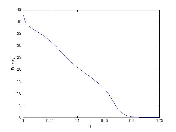
Fig. 1: Decay of the numerical energy $J^{h}_{\epsilon}(u_{h}^{\ell})$ of Test 1.

Figure 2 displays four snapshots at four fixed time points of the zero-level set of the numerical solution $u^{\epsilon,h,k}$ with four different $\epsilon$. They clearly indicate that at each time point the zero-level set converges to the mean curvature flow $\Gamma_{t}$ as $\epsilon$ tends to zero. It also shows that the zero-level set evolves faster in time for larger $\epsilon$.

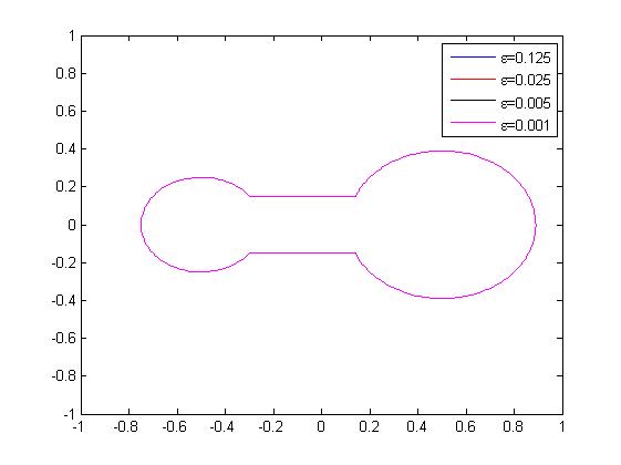
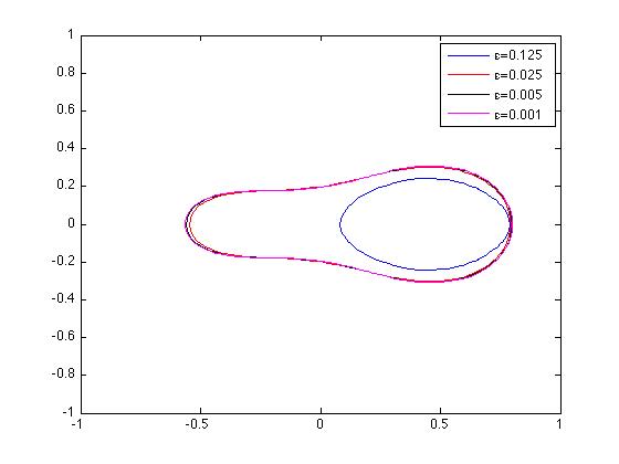
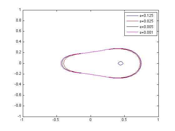
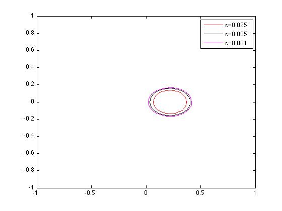
Fig. 2: Test 1: Snapshots of the zero-level set of $u^{\epsilon,h,k}$ at time $t=0,0.06,0.09,0.2$ and $\epsilon=0.125,0.025,0.005,0.001$.

$\mathbf{Test\,2.}$ Consider the Allen-Cahn problem (1)-(4) with the following initial condition:

$$u_{0}(x,y)=\begin{cases}\tanh(\frac{1}{\sqrt{2}\epsilon}(\text{min}\{d_{1},d_{2}\})),&\text{if}\ \frac{x^{2}}{0.04}+\frac{y^{2}}{0.36}\geq 1,\frac{x^{2}}{0.36}+\frac{y^{2}}{0.04}\geq 1,\\ &\ \text{or}\ \frac{x^{2}}{0.04}+\frac{y^{2}}{0.36}\leq 1,\frac{x^{2}}{0.36}+\frac{y^{2}}{0.04}\leq 1,\\ \tanh(\frac{1}{\sqrt{2}\epsilon}(-\text{min}\{d_{1},d_{2}\})),&\text{if}\ \frac{x^{2}}{0.04}+\frac{y^{2}}{0.36}<1,\frac{x^{2}}{0.36}+\frac{y^{2}}{0.04}>1,\\ &\ \text{or}\ \frac{x^{2}}{0.04}+\frac{y^{2}}{0.36}>1,\frac{x^{2}}{0.36}+\frac{y^{2}}{0.04}<1.\\ \end{cases}$$

Here $d_{1}(x)$ and $d_{2}(x)$ stand for, respectively, the distance functions to the two ellipses. We note that the above $u_{0}$ has the desired form as stated in Proposition 2.

Table 2 shows the spatial $L^{2}$ and $H^{1}$-norm errors and convergence rates, which are consistent with what are proved for the linear element in the convergence theorem.

	$L^{\infty}(L^{2})$ error	$L^{\infty}(L^{2})$ order	$L^{2}(H^{1})$ error	$L^{2}(H^{1})$ order
$h=0.4\sqrt{2}$	0.09186		0.29686
$h=0.2\sqrt{2}$	0.03670	1.3237	0.16331	0.8622
$h=0.1\sqrt{2}$	0.00911	2.0103	0.07603	1.1030
$h=0.05\sqrt{2}$	0.00276	1.7228	0.03740	1.0235
$h=0.025\sqrt{2}$	0.00071	1.9588	0.01846	1.0186

Table 2: Spatial errors and convergence rates of Test 2.

Figure 3 plots the change of the discrete energy $J^{h}_{\epsilon}(u_{h}^{\ell})$ in time, which should decrease according to (35). This graph clearly confirms this decay property.

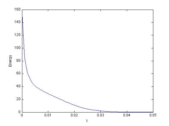
Fig. 3: Decay of the numerical energy $J^{h}_{\epsilon}(u_{h}^{\ell})$ of Test 1.

Like in Figure 2, Figure 4 displays four snapshots at four fixed time points of the zero-level set of the numerical solution $u^{\epsilon,h,k}$ with four different $\epsilon$. Once again, we observe that at each time point the zero-level set converges to the mean curvature flow $\Gamma_{t}$ as $\epsilon$ tends to zero, and the zero-level set evolves faster in time for larger $\epsilon$.

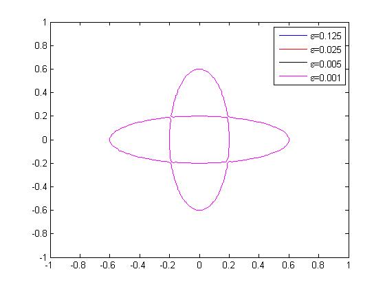
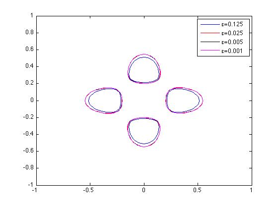
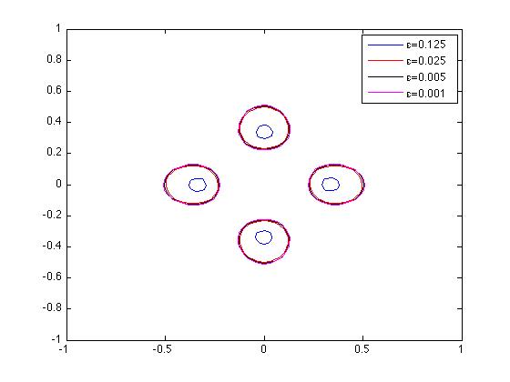
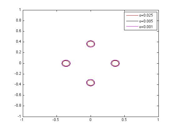
Fig. 4: Test 2: Snapshots of the zero-level set of $u^{\epsilon,h,k}$ at time $t=0,6\times 10^{-3},1.2\times 10^{-2},2\times 10^{-2}$ and $\epsilon=0.125,0.025,0.005,0.001$.

References

• [1] R. A. Adams, Sobolev Spaces, Academic Press, New York, 2003.
• [2] S. Allen and J. W. Cahn, A microscopic theory for antiphase boundary motion and its application to antiphase domain coarsening, Acta Metall., 27, 1084–1095 (1979).
• [3] S. Bartels, R. Múller, and C. Ortner, Robust a priori and a posteriori error analysis for the approximation of Allen-Cahn and Ginzburg-Landau equations past topological changes. submitted.
• [4] G. Bellettini and M. Paolini, Quasi-optimal error estimates for the mean curvature flow with a forcing term, Diff. Integr. Eqns, 8(4), 735–752 (1995).
• [5] Y. G. Chen, Y. Giga, and S. Goto, Uniqueness and existence of viscosity solutions of generalized mean curvature flow equations, Proc. Japan Acad. Ser. A Math. Sci., 65(7), 207–210 (1989).
• [6] X. Chen, Spectrum for the Allen-Cahn, Cahn-Hilliard, and phase-field equations for generic interfaces, Comm. PDEs, 19(7-8), 1371–1395 (1994).
• [7] Z. Chen and H, Chen, Pointwise error estimates of discontinuous Galerkin methods with penalty for second-order elliptic problems, SIAM J.Numer. Anal.,42,1146–1166 (2004).
• [8] C. M. Elliott, Approximation of curvature dependent interface motion, in The State of the Art in Numerical Analysis, pp. 407–440. Oxford University Press, 1997.
• [9] D. J. Eyre, An unconditional stable one-step scheme for gradient systems, unpublished.
• [10] L. C. Evans, H. M. Soner, and P. E. Souganidis, Phase transitions and generalized motion by mean curvature, Comm. Pure Appl. Math., 45(9), 1097–1123(1992).
• [11] X. Feng, Y. He, and C. Liu, Analysis of finite element approximations of a phase field model for two phase fluids, Math. Comp., 76, 539–571 (2007).
• [12] X. Feng and A. Prohl, Numerical analysis of the Allen-Cahn equation and approximation for mean curvature flows, Numer. Math., 94, 33–65 (2003).
• [13] X. Feng and H. Wu, A posteriori error estimates and an adaptive finite element algorithm for the Allen-Cahn equation and the mean curvature flow, J. Sci. Comput., 24(2), 121–146 (2005).
• [14] T. Ilmanen, Convergence of the Allen-Cahn equation to Brakke’s motion by mean curvature, J. Diff. Geom., 38(2), 417–461 (1993).
• [15] O. Karakashian and F. Pascal, Adaptive discontinuous Galerkin approximations of second order elliptic problems, Proceedings of European Congress on Computational Methods in Applied Sciences and Engineering, 2004.
• [16] D. Kessler, R. H. Nochetto, and A. Schmidt, A posteriori error control for the Allen-Cahn problem: circumventing Gronwall’s inequality, Math. Model. Numer. Anal., 38, 129–142 (2004).
• [17] G. B. McFadden, Phase field models of solidification, Contemporary Mathematics, 295, 107–145 (2002).
• [18] R. H. Nochetto and C. Verdi, Convergence past singularities for a fully discrete approximation of curvature-driven interfaces, SIAM J. Numer. Anal.,34(2), 490–512 (1997).
• [19] B. G. Pachpatte, Inequalities for Finite Difference Equations, Chapman & Hall/CRC Pure and Applied Mathematics, vol. 247, CRC Press, 2001.
• [20] B. Rivière, Discontinuous Galerkin Methods for Solving Elliptic and Parabolic Equations, SIAM, 2008.