Parallel Magnetic Resonance Imaging
as Approximation in a Reproducing Kernel Hilbert Space

Abstract

In Magnetic Resonance Imaging (MRI) data samples are collected in the spatial frequency domain (k-space), typically by time-consuming line-by-line scanning on a Cartesian grid. Scans can be accelerated by simultaneous acquisition of data using multiple receivers (parallel imaging), and by using more efficient non-Cartesian sampling schemes. To understand and design k-space sampling patterns, a theoretical framework is needed to analyze how well arbitrary sampling patterns reconstruct unsampled k-space using receive coil information. As shown here, reconstruction from samples at arbitrary locations can be understood as approximation of vector-valued functions from the acquired samples and formulated using a Reproducing Kernel Hilbert Space (RKHS) with a matrix-valued kernel defined by the spatial sensitivities of the receive coils. This establishes a formal connection between approximation theory and parallel imaging. Theoretical tools from approximation theory can then be used to understand reconstruction in k-space and to extend the analysis of the effects of samples selection beyond the traditional image-domain g-factor noise analysis to both noise amplification and approximation errors in k-space. This is demonstrated with numerical examples.

Keywords: Reproducing Kernel Hilbert Space, Magnetic Resonance Imaging, Image Reconstruction, Approximation, Inverse Problems, Non-Cartesian Sampling

1 Introduction

Magnetic Resonance Imaging (MRI) is a non-invasive tomographic imaging technique with many applications in medicine and biomedical research. Because it is based on serial scanning of the spatial frequency domain (known as k-space) by switching of magnetic field gradients, it is rather time consuming and susceptible to motion artifacts. Parallel MRI uses multiple receivers simultaneously to accelerate the measurement process. Different receive coils exhibit different spatial sensitivity profiles. Because receive coils’ different spatial sensitivity profiles provide additional information about the spatial origin of the signal, the signal can be restored from data which has been sampled below the Nyquist limit [1, 2, 3].

Most naturally, image reconstruction can be formulated as an inverse problem as in SENSE, where the image is estimated from the acquired data by solving a linear signal model [4, 2, 5, 6]. The conditioning of this system depends critically on the number and positions of the acquired samples. Although using local approximations in k-space, the earlier SMASH method is based on the same fundamental principles as SENSE. A classical review of parallel imaging methods and a discussion of the relationship between SENSE and SMASH can be found in [7]. The reconstruction from non-Cartesian (scattered) samples can also be formulated as an inverse problem and can be solved exactly in a continuous Hilbert space formulation [8, 9] or more commonly using discretization and efficient gridding techniques [10, 11, 12, 13]. Non-Cartesian sampling can be combined with SENSE [5] and other advanced reconstruction algorithms (see [14, 15, 16, 17] for recent examples).

Because the reconstruction problem is well-posed for sufficiently dense and regular sampling, a different two-step reconstruction strategy is applied in certain k-space methods. Using the acquired samples, a vector-valued function is approximated on a Nyquist-sampled grid in k-space, which is then transformed to the image domain for all coils and only then combined into a final image. This strategy is used in coil-by-coil SMASH [18], GRAPPA, and similar methods, which have first been formulated for sampling on a grid and later extended to non-Cartesian sampling in various ways [19, 20, 21, 22, 23, 24, 25, 26, 15].

Previously, we have shown how both types of reconstruction constrain the data to a subspace spanned by the spatial sensitivity profiles of the receive coils [27]. In this work, we extend this idea by showing that parallel imaging from arbitrary - Cartesian as well as non-Cartesian - samples in k-space can be expressed formally as the approximation problem in a Reproducing Kernel Hilbert Space (RKHS) [28, 29]. A RKHS is a Hilbert space of functions where the point-evaluation functionals are continuous, i.e. they are compatible with the norm of the Hilbert space. This is a natural and intuitive property that means functions close in norm difference are also close at each point and provides the additional structure necessary to describe sampling in a Hilbert space setting. A RKHS is uniquely characterized by its reproducing kernel. In parallel MRI, the reproducing kernel is determined by the coil sensitivities, which can be derived directly from the basic signal equation. While some related ideas can be found in the literature, i.e. GRAPPA has been related to the geostatistical framework of Kriging [30] and the “kernel trick” known from support vector machines has been used to develop a non-linear variant of GRAPPA [31], a full mathematical description has so far not been available. This gap is closed in the present work by formulating parallel imaging in the framework of approximation theory. It does not only provide an optimal interpolation formula as a (theoretical) basis for image reconstruction in parallel MRI, but also enables a much deeper understanding of the reconstruction problem itself. In particular, the power function [32] and Frobenius norm maps, that naturally come out of the RKHS formulation, give local bounds of the approximation error and about noise amplification in multi-coil k-space or - with a small extension - directly for the Fourier transform of the image. Both functions depend on the sample points but not on the data and can be used to study the effect of sample selection on the reconstruction error. This is demonstrated with numerical examples.

2 Theory

2.1 Overview

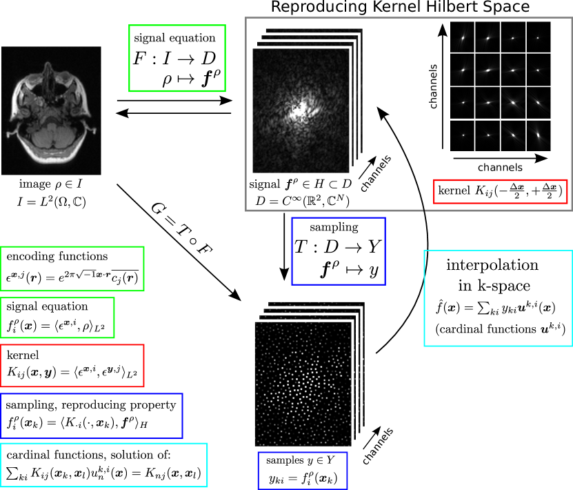
Figure 1: Image reconstruction for parallel MRI as approximation in a reproducing kernel Hilbert space.

An overview of the theory developed in the following is shown in Figure 1. Please refer to Appendix 7.1 for some comments about the notation and to Table 1 for a list of important symbols.

We consider parallel imaging as an inverse problem with a linear forward model $F:I\rightarrow D$, which maps from a Hilbert space of images $I$ to a data space $D$. The range of $F$ is the space of ideal signals $H\subset D$. From the data space a set $y\in Y$ of samples are acquired, which is described by a sampling operator $T$. Then, the general setting is the following:

$$\begin{array}[]{cccc}I&\xrightarrow{F}&H&\subset D\\ &\searrow_{G}&\downarrow_{T}&\\ &&Y&\end{array}$$

Here, $G=T\circ F$. A general formulation of linear inverse problems with discrete data can be found in [8]. The inverse problem can be solved by computing a regularized least-squares solution by minimizing a functional

$$\rho_{\alpha}=G^{\dagger}_{\alpha}y=\operatorname*{argmin}_{\hat{\rho}}\|G\hat{\rho}-y\|_{2}^{2}+\alpha R(\hat{\rho})$$ (1)

with a suitable regularization term $R$. In the limit $\alpha\rightarrow 0$, this yields a minimum-norm least-squares solution (MNLS). In general, the mapping $F$ is injective and has a stable inverse defined on its range $H$. Alternatively to solving the inverse problem directly, one can approximate a function $\boldsymbol{\hat{f}}\in H$ from the data $y\in Y$ and obtain a solution by computing $\hat{\rho}=F^{-1}\hat{\boldsymbol{f}}$.

$\boldsymbol{x},\boldsymbol{y}$	k-space positions
$S$	finite set of sample locations
$\boldsymbol{x}_{k},\boldsymbol{y}_{l}$	indexed sample locations in $S$
$i,j,n$	indices used for vector components (channels)
$H$	Hilbert space of vector-valued k-space functions
$\boldsymbol{K}^{\boldsymbol{x},i}(\boldsymbol{y})$	representer of evaluation of channel $i$ at $\boldsymbol{x}$
$K_{ij}(\boldsymbol{x},\boldsymbol{y})$	matrix-valued kernel
$M_{ki,lj}$	kernel matrix
$\boldsymbol{u}^{k,i}(\boldsymbol{x})$	cardinal functions
$\langle\cdot,\cdot\rangle_{H}$	inner product in $H$
$P_{n}(\boldsymbol{x})$	Power function for channel $n$
$\Omega$	the field of view (FOV)
$L^{2}(\Omega,\mathbb{C})$	square-integrable functions on $\Omega$
$\boldsymbol{r}$	image-domain position
$c_{j}(\boldsymbol{r})$	coil sensitivity map for channel $j$
$\epsilon^{\boldsymbol{x},i}(\boldsymbol{r})$	encoding functions
$\rho(\boldsymbol{r})$	image
$\overline{(\cdot)}$	complex conjugate

Table 1: Important symbols.

2.2 Parallel Magnetic Resonance Imaging

We begin with the standard setup of the parallel imaging problem. For concreteness, we consider two-dimensional imaging. Let the magnetization image $\rho:\mathbb{R}^{2}\rightarrow\mathbb{C}$ belong to the space $L^{2}(\Omega,\mathbb{C})$ of square-integrable functions with compact support $\Omega$ on a subset of the plane called the field of view (FOV). The forward operator $F$ maps magnetization images to smooth signals in k-space:

$$F:L^{2}(\Omega,\mathbb{C}) \rightarrow C^{\infty}(\mathbb{R}^{2},\mathbb{C}^{N})$$ (2)

$$\rho \mapsto\boldsymbol{f}^{\rho}=F\rho$$ (3)

Each vector component, which is the signal of one of $N$ receive coils, is given by the signal equation:

$$f_{j}^{\rho}(\boldsymbol{x})=\int_{\Omega}d\boldsymbol{r}\,\rho(\boldsymbol{r}){c_{j}(\boldsymbol{r})e^{-2\pi\sqrt{-1}\boldsymbol{x}\cdot\boldsymbol{r}}}\quad\quad\quad 1\leq j\leq N$$ (4)

In words, the $j^{\mathrm{th}}$ component of the vector-valued function $\boldsymbol{f}^{\rho}$ is the Fourier transform of coil $j$’s image. The k-space signals are smooth because they are Fourier transforms of compactly supported functions. The coil sensitivities $c_{j}$ are generally smooth, complex-valued functions in image space describing the spatial sensitivity profiles of each receiver coil. In areas where all coil sensitivities vanish simultaneously, no information about the image can be recovered. Without loss of generality, we will simply assume that the definition of $\Omega$ excludes such areas. Using the inner product definition

$$\langle\rho,\sigma\rangle_{L^{2}}=\int_{\Omega}d\boldsymbol{r}\,\overline{\rho(\boldsymbol{r})}\sigma(\boldsymbol{r})$$ (5)

and the encoding functions $\epsilon^{\boldsymbol{x},j}(\boldsymbol{r})=e^{2\pi\sqrt{-1}\boldsymbol{x}\cdot\boldsymbol{r}}\overline{c_{j}(\boldsymbol{r})}$ [2], we can write $f_{j}^{\rho}(\boldsymbol{x})=\langle\epsilon^{\boldsymbol{x},j},\rho\rangle_{L^{2}}$. During the measurement process samples at a finite number of locations $\boldsymbol{x}_{k}\in S\subset\mathbb{R}^{2}$ are collected. Samples can be assumed to be corrupted by i.i.d. complex Gaussian white noise. Although in practice receive channels might have different noise levels and correlations, this can be removed by a prewhitening step and a change-of-variable transformation of the coil sensitivities [5].

2.3 Reproducing Kernel Hilbert Space

The vector-valued functions considered in parallel imaging have the particular structure specified in Equation 4. We now encapsulate this structure within a reproducing kernel Hilbert space $H$ with a matrix-valued kernel [33, 34].

Let $X$ be a set of points, and $H$ a Hilbert space of vector-valued functions on $X$. $H$ is an RKHS if the point-evaluation functionals $L^{\boldsymbol{x}}:H\rightarrow\mathbb{C}^{N}$, $\boldsymbol{f}\mapsto\boldsymbol{f}(\boldsymbol{x})$ are continuous for all $\boldsymbol{x}\in X$. From the Riesz representation theorem, it then follows that there are unique functions $\boldsymbol{K}^{\boldsymbol{x},i}\in H$ for each $\boldsymbol{x}\in X$ and each vector component $1\leq i\leq N$ such that $f_{i}(\boldsymbol{x})=\left\langle\boldsymbol{K}^{\boldsymbol{x},i},\boldsymbol{f}\right\rangle_{H}$. As before, we define the inner product $\langle\cdot,\cdot\rangle_{H}$ in $H$ to be conjugate linear in the first argument. The functions $\boldsymbol{K}^{\boldsymbol{x},i}$ are called representers of evaluation. They span $H$, but do not generally form a basis. If a series of functions $\boldsymbol{f}^{n}$ converges to $\boldsymbol{f}^{\star}$ in the Hilbert space norm, then for any $\boldsymbol{x}\in X$ and vector component $1\leq i\leq N$, we have

$$|f_{i}^{n}(\boldsymbol{x})-f^{\star}_{i}(\boldsymbol{x})| =|\left\langle\boldsymbol{K}^{\boldsymbol{x},i},\boldsymbol{f}^{n}-\boldsymbol{f}^{\star}\right\rangle_{H}|$$

$$\leq\|\boldsymbol{K}^{\boldsymbol{x},i}\|_{H}\|\boldsymbol{f}^{n}-\boldsymbol{f}^{\star}\|_{H}\leavevmode\nobreak\ .$$ (6)

This means that convergence in norm implies point-wise convergence and that local bounds can be obtained using information about the representers.

The structure of the space can then be described by a positive-definite matrix-valued kernel $K:X\times X\rightarrow\mathbb{C}^{N\times N}$ such that an element of the kernel $K_{ij}(\boldsymbol{x},\boldsymbol{y})=\left\langle\boldsymbol{K}^{\boldsymbol{x},i},\boldsymbol{K}^{\boldsymbol{y},j}\right\rangle_{H}$. A RKHS is uniquely characterized by its positive-definite kernel and to every positive-definite kernel there is a unique RKHS. From the definition of the representers of evaluation it follows that $K_{ij}(\boldsymbol{x},\boldsymbol{y})=K_{i}^{\boldsymbol{y},j}(\boldsymbol{x})$, the $i^{\mathrm{th}}$ component of the vector-valued function $\boldsymbol{K}^{\boldsymbol{y},j}$ that evaluates the $j^{\mathrm{th}}$ component of a function at $\boldsymbol{y}$. Thus, the reproducing property holds:

$$f_{j}(\boldsymbol{y}) =\left\langle{K}_{\cdot j}(\cdot,\boldsymbol{y}),\boldsymbol{f}\right\rangle_{H}\qquad\forall\boldsymbol{y}\in X$$ (7)

Applying this framework to parallel MRI, the space $H$ is the range of $F$, i.e. it consists of ideal signals $\boldsymbol{f}$ on $\mathbb{R}^{2}$ given by Equation 4 for all possible images $\rho\in L^{2}(\Omega,\mathbb{C})$. We can assume that at least one of the coil sensitivities $c_{j}$ is non-zero at each point $\boldsymbol{r}\in\Omega$. Then $F$ can be inverted by applying an inverse Fourier transform (practical computation can be done on a Nyquist-sampled grid) and dividing by a non-zero $c_{i}$. This enables the following definition of an inner product in $H$:

$$\left\langle\boldsymbol{f},\boldsymbol{g}\right\rangle_{H}:=\langle F^{-1}\boldsymbol{f},F^{-1}\boldsymbol{g}\rangle_{L^{2}}$$ (8)

With this inner product, we formulate our main result:

Theorem: The space $H$ of ideal multi-channel signals in MRI is a RKHS with kernel:

$$K_{ij}(\boldsymbol{x},\boldsymbol{y}) =\langle\epsilon^{\boldsymbol{x},i},\epsilon^{\boldsymbol{y},j}\rangle_{L^{2}}$$

$$=\int_{\Omega}d\boldsymbol{r}\,e^{-2\pi\sqrt{-1}(\boldsymbol{x}-\boldsymbol{y})\cdot\boldsymbol{r}}c_{i}(\boldsymbol{r})\overline{c_{j}(\boldsymbol{r})}$$ (9)

Proof.

We must show two properties: For each $\boldsymbol{y}\in\mathbb{R}^{2}$ and $1\leq j\leq N$ the $\boldsymbol{K}^{\boldsymbol{y},j}$ must lie in $H$, and $\left\langle\boldsymbol{K}^{\boldsymbol{y},j},\boldsymbol{f}\right\rangle_{H}=f_{j}(\boldsymbol{y})$. We observe that the kernel can be obtained by applying $F$ to the encoding functions $\epsilon^{\boldsymbol{y},j}$:

$$\left(F\epsilon^{\boldsymbol{y},j}\right)_{i}(\boldsymbol{x})=\langle\epsilon^{\boldsymbol{x},i},\epsilon^{\boldsymbol{y},j}\rangle_{L^{2}}=K_{ij}(\boldsymbol{x},\boldsymbol{y})=K^{\boldsymbol{y},j}_{i}(\boldsymbol{x})$$ (10)

Thus, $\boldsymbol{K}^{\boldsymbol{y},j}$ is in the range of $F$ and therefore in $H$. The second property follows directly from the definition of the inner product. For every $\boldsymbol{f}^{\rho}=F\rho$, it follows:

$$\left\langle\boldsymbol{K}^{\boldsymbol{y},j},\boldsymbol{f}^{\rho}\right\rangle_{H}=\left\langle F\epsilon^{\boldsymbol{y},j},F\rho\right\rangle_{H}=\left\langle\epsilon^{\boldsymbol{y},j},\rho\right\rangle_{L^{2}}=f_{j}^{\rho}(\boldsymbol{y})$$ (11)

∎

In words, $K_{ij}(\boldsymbol{x},\boldsymbol{y})$ captures the similarity between encoding functions $\epsilon^{\boldsymbol{x},i}$ and $\epsilon^{\boldsymbol{y},j}$. Note that $K_{ij}(\boldsymbol{x},\boldsymbol{y})=K_{ij}(\boldsymbol{x}+\Delta,\boldsymbol{y}+\Delta)$, and so the kernel is shift invariant. It should be noted that there is some freedom in the choice of the inner product. Using a different inner product will lead to a different kernel. The inner product used here corresponds to the inner product of the Hilbert space of images. As shown later, the final reconstruction will then be optimal with respect to this norm.

Having characterized the multi-channel k-space of ideal signals as an RKHS with the shift-invariant kernel given in Equation 2.3, we can now proceed to describe sampling and reconstruction in this framework.

2.4 Sampling and Reconstruction

Sampling and reconstruction from arbitrary samples can be described in the framework of approximation theory (see [29] as general reference). Because it is usually formulated for the scalar case only, we summarize the main results using our notation.

Samples are collected at a finite number of locations $\boldsymbol{x}_{k}\in S\subset\mathbb{R}^{2}$. Ideal samples of $\boldsymbol{f}\in H$ are then given by the inner product evaluations $\boldsymbol{f}_{i}(\boldsymbol{x}_{k})=\left\langle\boldsymbol{K}^{\boldsymbol{x}_{k},i},\boldsymbol{f}\right\rangle_{H}$ for all $i\in 1,\cdots,N$ and $\boldsymbol{x}_{k}\in S$. Assuming no measurement error, a solution to the reconstruction problem is usually defined as the function $\boldsymbol{\hat{f}}\in H$ of smallest norm which interpolates $\boldsymbol{f}$ at the sample locations, i.e. $\boldsymbol{\hat{f}}(\boldsymbol{x}_{l})=\boldsymbol{f}(\boldsymbol{x}_{l})$. We first define a measurement subspace $H_{S}\subset H$ that is spanned by $\boldsymbol{K}^{\boldsymbol{x}_{k},i}$ for all $\boldsymbol{x}_{k}\in S,\>1\leq i\leq N$. Thus, any function $\boldsymbol{f}\in H_{S}$ can be represented as

$$\boldsymbol{f}=\sum_{k=1}^{|S|}\sum_{i=1}^{N}a_{k,i}\boldsymbol{K}^{\boldsymbol{x}_{k},i}\leavevmode\nobreak\ .$$ (12)

This subspace turns out to be the right space for interpolation: In the absence of errors, all functions in $H_{S}$ can be recovered exactly (see below), while the functions $\boldsymbol{f}^{\perp}\in H_{S}^{\perp}$ are those for which the samples provide no information, i.e. $\boldsymbol{f}^{\perp}(S)=\{0\}$ (by Eq. 7). The minimum-norm interpolant $\boldsymbol{\hat{f}}$ for $\boldsymbol{f}\in H$ for the samples $S$ is the projection $\boldsymbol{f}^{\parallel}$ of $\boldsymbol{f}$ onto $H_{S}$. To compute this projection, we could directly solve for coefficients $a_{k,i}$ such that ${\boldsymbol{\hat{f}}}(\boldsymbol{x}_{k})=\boldsymbol{f}(\boldsymbol{x}_{k})$ for $\boldsymbol{x}_{k}\in S$.

Instead, we formulate a generic solution which only depends on the sample locations and not on the data. The kernel matrix $M\in\mathbb{C}^{|S|N\times|S|N}$ is constructed by evaluating the kernel at all sample positions $\boldsymbol{x}_{k}\in S$, i.e. $M_{ki,lj}=K_{ij}(\boldsymbol{x}_{k},\boldsymbol{x}_{l})$. Here, the pairs of indices $k$, $i$ and $l$, $j$ have each been combined to obtain the two indices of the matrix. For each point $\boldsymbol{x}$, interpolation weights called cardinal functions $\boldsymbol{u}^{k,i}(\boldsymbol{x})$ can then be computed by solving a linear system of equations:

$$\sum_{k=1}^{|S|}\sum_{i=1}^{N}M_{ki,lj}\,\boldsymbol{u}^{k,i}(\boldsymbol{x})=\boldsymbol{K}^{\boldsymbol{x}_{l},j}(\boldsymbol{x})$$ (13)

The cardinal functions are independent from $\boldsymbol{f}$ and interpolate functions from $H$ according to (see Appendix 7.2)

$$\boldsymbol{\hat{f}}(\boldsymbol{x}) =\sum_{k=1}^{|S|}\sum_{i=1}^{N}f_{i}(\boldsymbol{x}_{k})\boldsymbol{u}^{k,i}(\boldsymbol{x})\leavevmode\nobreak\ .$$ (14)

In principle, parallel MRI reconstruction can be performed using this formula: The interpolation formula can be used to compute samples on a Nyquist-sampled grid followed by an FFT algorithm to compute an image for each coil. Evaluation of Equation 13 requires the solution of the linear system of equations of size $|S|N\times|S|N$ for each point of the Nyquist-sampled grid. Although all solutions can be obtained efficiently after computation of the pseudo-inverse (or Cholesky decomposition) of the kernel matrix, this is still too expensive for image reconstruction in clinical applications due to the size of this matrix. Nevertheless, this formula is closely related to more efficient practical algorithms such as GRAPPA, which are based on an approximation.

2.5 Approximation Error and Noise

A useful tool to estimate approximation errors is the power function $\boldsymbol{P}$ [32]. It yields point-wise bounds of the approximation error:

$$|\boldsymbol{f}_{n}(\boldsymbol{x})-\boldsymbol{\hat{f}}_{n}(\boldsymbol{x})|^{2}\leq\|\boldsymbol{f}\|_{H}^{2}\cdot P^{2}_{n}(\boldsymbol{x})$$ (15)

The power function depends only on the sample locations and is independent from the data values. It is given in terms of the kernel and the cardinal functions (see Appendix 7.3). This concept enables us to understand how good our sample set $S$ is for approximating $\boldsymbol{f}$ at unacquired points. A single combined power function can be obtained as the root of sum of squares of the power functions for all coils. A large power function indicates that we should expect a large approximation error at this point. A small value of the power function means that the function is approximated well from the available samples and that a new sample at $\boldsymbol{x}$ would not provide much information.

Another quantity of interest is the Frobenius norm of the local reconstruction operator:

$$n_{n}(\boldsymbol{x})=\sqrt{\sum_{k=1}^{|S|}\sum_{i=1}^{N}\left|\boldsymbol{u}^{k,i}_{n}(\boldsymbol{x})\right|^{2}}$$ (16)

It relates to the stability of the interpolation, describing the local noise amplification in k-space for each individual coil (or for all coils using a combined map). This yields different and complementary information to the g-factor maps in the image domain [2, 35]. While the g-factor map yields information about how noise affects the final reconstructed image, these new noise amplification maps yield useful information about the source of the noise in k-space and can guide the design of optimal sampling patterns. A related quantity is the classical Lebesgue function, which is defined as

$$l_{n}(\boldsymbol{x})=\sum_{k=1}^{|S|}\sum_{i=1}^{N}\left|\boldsymbol{u}^{k,i}_{n}(\boldsymbol{x})\right|\leavevmode\nobreak\ .$$ (17)

Its maximum is the Lebesgue constant, which can be used to bound the interpolation error in the maximum norm when the error of the data is bounded (for example, see [36]).

2.6 Minimum-Norm Reconstruction

Eq. 1 defines the MNLS solution of SENSE in the continuous (not discretized) space of image. It is more precise than a conventional SENSE reconstruction using dirac distributions as voxel functions, which is affected by truncation artifacts [37]. A MNLS reconstruction in the image domain can be computed directly [7] or approximated efficiently by computation on an image-domain grid with higher resolution [38, 39, 40].

With our choice of the inner product, the k-space recovered with Eq. 14 corresponds to this MNLS reconstruction of the image. Solving for the cardinal functions (Eq. 13) using the pseudo-inverse $M^{\dagger}$ of the kernel matrix and inserting into the interpolation formula (Eq. 14) yields:

$$\hat{\boldsymbol{f}}=\sum_{l=1}^{|S|}\sum_{j=1}^{N}\boldsymbol{K}^{\boldsymbol{x}_{l},j}\sum_{k=1}^{|S|}\sum_{i=1}^{N}M^{\dagger}_{lj,ki}f_{i}(\boldsymbol{x}_{k})$$ (18)

Expanding the relations

$$M_{ki,lj} =K_{ij}(\boldsymbol{x}_{k},\boldsymbol{x}_{l})=\langle\epsilon^{\boldsymbol{x}_{k},i},\epsilon^{\boldsymbol{x}_{l},j}\rangle_{L^{2}}$$ (19)

$$\boldsymbol{K}^{\boldsymbol{x}_{l},j} =F\epsilon^{\boldsymbol{x}_{l},j}$$ (20)

and noting that the result can be re-written using the forward operator

$$G:L^{2}(\Omega,\mathbb{C}) \rightarrow\mathbb{C}^{|S|N}$$ (21)

$$\rho \mapsto y_{ki}=\langle\epsilon^{\boldsymbol{x}_{k},i},\rho\rangle_{L^{2}}$$ (22)

and its adjoint $G^{H}$, one obtains $M=GG^{H}$ and further

$$\hat{\boldsymbol{f}} =FG^{H}\left(GG^{H}\right)^{\dagger}y$$ (23)

$$=FG^{\dagger}y\leavevmode\nobreak\ .$$ (24)

From this formulation it is directly evident that the k-space signal interpolated with Eq. 14 is the same as the signal predicted with the operator $F$ from the MNLS solution $G^{\dagger}y$ of the continuous (not discretized in the image domain) SENSE problem. No discretization errors arise, because the kernel matrix $M$, i.e. $GG^{H}$, is a finite-dimensional matrix even for the continuous case. Of course, this is not a unique feature of the proposed formulation: The relation $G^{H}\left(GG^{H}\right)^{\dagger}=G^{\dagger}$ used in the last equation can be applied in reverse to the SENSE problem to directly compute the MNLS solution without discretization errors [7]. The same idea has also been proposed earlier for the reconstruction of non-Cartesian data from a single coil [9].

2.7 Relationship to GRAPPA

Equation 14 is similar to the reconstruction part of the GRAPPA algorithm, with the GRAPPA weights corresponding to the cardinal functions. To make actual computation feasible, GRAPPA uses only samples in a small patch near a given point. If $S_{\boldsymbol{x}}\subset S$ is the set of samples near $\boldsymbol{x}$ which are used for reconstruction, then the GRAPPA reconstruction $\boldsymbol{\hat{f}}_{G}$ is given by:

$$\boldsymbol{\hat{f}}_{G}(\boldsymbol{x})=\sum_{k|\boldsymbol{x}_{k}\in S_{\boldsymbol{x}}}\sum_{i=1}^{N}f_{i}(\boldsymbol{x}_{k})\boldsymbol{w}^{k,i}(\boldsymbol{x})$$ (25)

The weights are determined with a calibration procedure. The calibration (and reconstruction) in the original GRAPPA method is restricted to samples on a Cartesian grid. Using shift invariance, the weights $\boldsymbol{w}^{k,i}(\boldsymbol{x})$ are learned by a least-squares fit at many different grid positions $\boldsymbol{x}_{t}\in C$ in a calibration region where all required samples (on the grid) have been acquired:

$$w_{j}^{k,i}(\boldsymbol{x})=\operatorname*{argmin}_{\hat{w}^{k,i}}\sum_{t=1}^{|C|}\Biggl{|}\sum_{k|\boldsymbol{x}_{k}\in S_{\boldsymbol{x}}}\sum_{i=1}^{N}f_{i}(\boldsymbol{x}_{t}+\underbrace{\boldsymbol{x}_{k}-\boldsymbol{x}}_{\Delta\boldsymbol{x}_{k}})\hat{w}^{k,i}-f_{j}(\boldsymbol{x}_{t})\Biggr{|}^{2}$$ (26)

The distance vectors $\Delta\boldsymbol{x}_{k}$ which appear in the sum for a specific target position $\boldsymbol{x}$ depend on the local sampling pattern. The least-squares problem can be solved explicitly using the normal equations. Because in GRAPPA only neighboring samples are used, it is useful to define a so-called calibration matrix, which is computed by sliding a small window through the calibration area and taking each patch as a row, i.e. $A_{t,ki}=f_{i}(\boldsymbol{x}_{t}+\Delta\boldsymbol{x}_{k})$ for all possible distance vectors $\Delta\boldsymbol{x}_{k}$ in a small patch. Assuming a special index $0$ with $\Delta\boldsymbol{x}_{0}=\bf 0$, i.e. $A_{t,0i}=f_{i}(\boldsymbol{x}_{t})$, the normal equations are given by (with $l$ such that $\Delta\boldsymbol{x}_{l}+\boldsymbol{x}\in S_{\boldsymbol{x}}$ and $j=1\cdots N$)

$$\sum_{k|\Delta\boldsymbol{x}_{k}+\boldsymbol{x}\in S_{\boldsymbol{x}}}\sum_{i=1}^{N}\sum_{t=1}^{|C|}\overline{A_{t,lj}}A_{t,ki}\,w_{h}^{k,i}(\boldsymbol{x}) =\sum_{t=1}^{|C|}\overline{A_{t,lj}}A_{t,0h}\leavevmode\nobreak\ .$$ (27)

Again, this relates to the present framework as this is Equation 13 expressed using relative distances and with a kernel matrix $M_{ki,lj}=\sum_{t}A_{t,ki}\overline{A_{t,lj}}$. This kernel matrix is related to an estimate of a truncated covariance function given by (assuming vanishing mean):

$$Cov_{ij}(\Delta\boldsymbol{x})=\frac{1}{|C|}\sum_{t=1}^{|C|}{f_{i}(\boldsymbol{x}_{t})}\overline{f_{j}(\boldsymbol{x}_{t}+\Delta\boldsymbol{x})}$$ (28)

Note, that due to the kernel’s shift invariance, the GRAPPA weights (or cardinal functions) in a local approximation of the interpolation formula (Eq. 14) are identical at positions in k-space which share the same local sampling pattern. In this way, computation time for (quasi-)periodic sampling can be reduced considerably.

In summary, the GRAPPA algorithm can be re-formulated and understood as function approximation in a RKHS. Instead of the optimal kernel, which has analytically been derived from the coil sensitivities in Equation 2.3, a different kernel (which corresponds to a different RKHS) related to the empirical covariance function is used. Reconstruction differs from the optimal formula by only using local samples for interpolation.

3 Numerical Examples

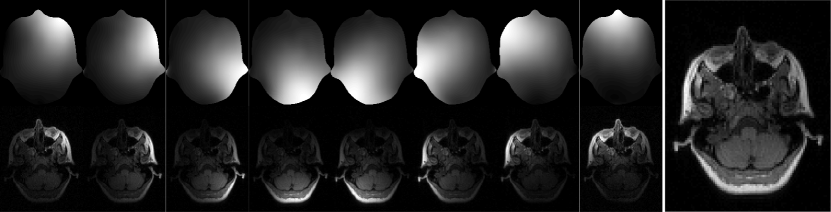
Figure 2: Top row: Spatial sensitivity maps for each channel of the receive coil (limited to the support of the object). Bottom row: Corresponding coil images computed by Fourier transform of each channel of the fully-sampled data. Right: Combined image computed as the pixel-wise root of the sum of absolute squares of all coil images.

3.1 Methods

Numerical experiments have been performed using a 2D slice of size $115\times 90$ extracted from a larger fully-sampled 3D data set of a human head acquired at 1.5 T using an eight-channel head coil (inversion-recovery prepared RF-spoiled 3D-FLASH, TR/TE = 12.2/5.2 ms, TI = 450 ms, FA = 20^∘, BW = 15 KHz). In order to demonstrate k-space interpolation from Cartesian and arbitrary, non-Cartesian samples, sampling patterns were generated on a k-space grid oversampled by $3\times$ in each dimension by zero-padding in the image domain. From this data set samples have been obtained using Cartesian, Poisson-disc, and uniform random sampling. Cartesian sampling used an undersampling of four in one phase-encoding direction ($4\times 1$) and of two in both phase-encoding directions ($2\times 2$). In addition, different CAIPIRINHA [41] patterns have been studied. The Poisson-disc radius used yielded 2494 samples corresponding to an acceleration factor about four relative to the original number of samples, and the uniform random sampling pattern was generated to match this number of samples.

Coil sensitivities have been estimated using ESPIRiT [27], which yields very accurate sensitivities up to point-wise normalization and a mask which defines the area with signal. From these coil sensitivities the kernel has been computed by evaluating Equation 2.3 using a zero-padded Fourier transform. To demonstrate reconstruction errors from interpolation errors only, i.e. excluding errors from noise, a synthetic data set was created: The fully-sampled data was combined into a single image and then data was simulated using the coil sensitivities.

For all sampling patterns, a kernel matrix has been constructed by evaluating the kernel at the sample positions. Especially when some samples are close together as in the random sampling pattern, corresponding rows and columns in the kernel matrix are very similar, and the condition number is large. For this reason, the inversion of the kernel matrix has to be stabilized with Tikhonov regularization in the presence of noise and numerical errors. The maximum eigenvalue as determined by power iteration of the kernel matrix was $51.0062$ for Cartesian $4\times 1$, $31.033$ for Cartesian $2\times 2$, $33.863$ for Poisson-disc, and $116.45$ for random sampling. For the CAIPIRINHA patterns the values were between $30.0936$ and $35.3207$. To avoid a large influence on the solution, Tikhonov regularization (ridge regression) was used with a much smaller parameter of $0.01$ for all experiments.

For each point on an oversampled and extended Cartesian grid, the cardinal and power functions have been computed. To reduce computation time, Equation 13 is solved by forward and backward substitution using a Cholesky decomposition of the kernel matrix. To estimate interpolation error and noise amplification at each position, a combined power function for all coils is computed by root of sum of squares and the cardinal functions are combined in the same way which yields the Frobenius norm of the local interpolation operator. Using the cardinal function, a Nyquist-sampled k-space has then been approximated from the acquired samples for synthetic and noisy data and transformed into coil images using an FFT.

The simulations were performed using Matlab (The MathWorks, Inc., Natick, MA) on a cluster with two quad-core Intel Xeon E5550 CPUs (2.67 GHz) per node. Computing the kernel matrix of size $\sim 20000^{2}$ and calculating the Cholesky decomposition took about two CPU hours. Solving for the cardinal functions for all interpolation points was broken into smaller parallel jobs to reduce runtime and memory use. To interpolate from the samples to the full $115\times 90$ grid took $\sim 350$ CPU hours and to interpolate over the $3\times$ oversampled and extended grid of size $405\times 330$ took about $\sim 4500$ CPU hours. Utilizing about $20$ parallel jobs on the cluster, this took about $6$ hours for the full grid and about $3$ days for the oversampled grid. All computations used double-precision floating-point arithmetic.

3.2 Results

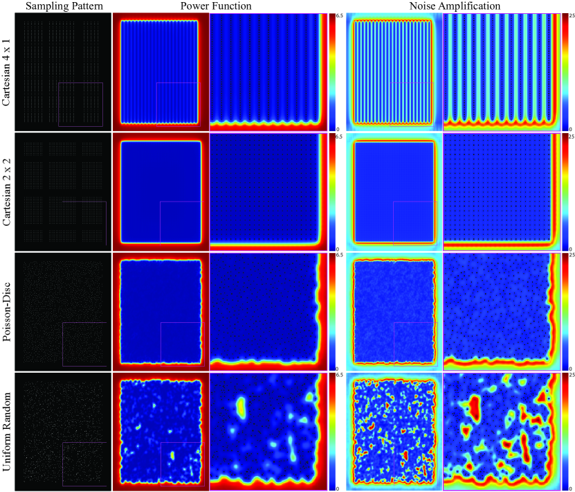
Figure 3: Sampling pattern, combined power function, and local noise amplification for Cartesian, Poisson-disc, and random sampling on an oversampled and extended grid. The maximum possible value for the power function is $6.5530$ in regions where no information is available. In the blown-up region of the lower-right corner sample positions are indicated by black dots.

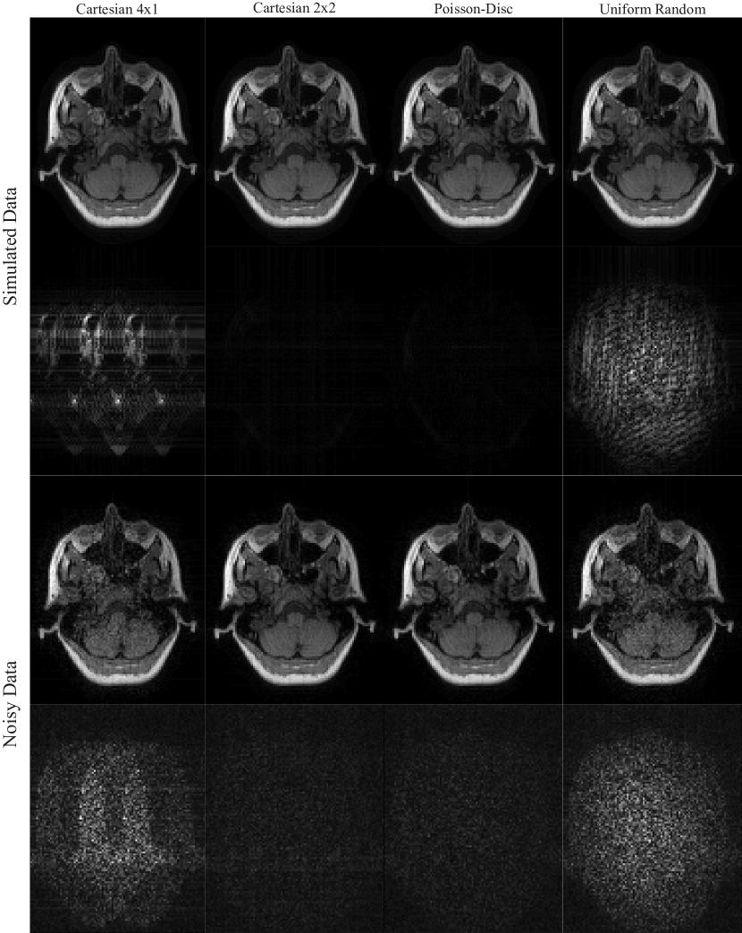
Figure 4: Reconstructed images and corresponding error maps for Cartesian, Poisson-disc, and uniform random sampling for simulated (top) and noisy data (bottom). All sampling schemes used an undersampling factor of 4. Error maps have been scaled by a factor of 40 (simulated) and 4 (noisy) to aid visibility.

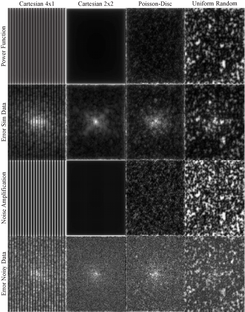
Figure 5: Theoretical power function and noise amplification maps as well as actual reconstruction errors in k-space for simulated and noisy data. Because energy of the error is much higher near the center of k-space, the maps have been raised to a power of $1/3$ for improved visualization of their structure. For this reason, please note that the relative intensity of the different maps is misleading.

Figure 2 shows the coil image and the corresponding sensitivity map for all receive channels as well as the combined image. Figure 3 shows the combined power function and the Frobenius norm of the cardinal functions for different sampling patterns. While for Cartesian $2\times 2$ and Poisson-disc sampling the power function is small everywhere inside the sampled region indicating that interpolation error is small, the situation is different for Cartesian $4\times 1$ and uniform random sampling: Where larger gaps appear in the sampling pattern, the power function has high values. The power functions themselves are bounded by the diagonal elements of the kernel. This bound is approached in regions where the cardinal functions go to zero, i.e. far from acquired samples, and corresponds to a situation where nothing is known about the k-space value. The bound for the combined power functions is $6.5530$ for the kernel used here. Consistent with this upper bound, the maximum values observed near the boundary in the computed maps are $6.4802$ for Cartesian $4\times 1$, $6.3921$ for Cartesian $2\times 2$, $6.3797$ for Poisson-disc, and $6.4277$ for uniform random sampling. Computing the maximum in a smaller inner region of size $305\times 230$ far from the boundary, the maximum values are $0.6154$, $0.05252$, $0.1087$, and $4.3303$, respectively. The last number highlights the fact that high values are attained even inside the sampled area for uniform random sampling. While the error bound for Poisson-disc sampling is twice as large as for the Cartesian $2\times 2$ pattern, it is still very small, i.e. $60\times$ smaller than the maximum which is obtained in unsampled regions. The reconstruction results (Fig. 4) for noise-less data confirm that the interpolation error is lower for Cartesian and Poisson-disc than for uniform random sampling. Cartesian $4\times 1$ performs worse than Cartesian $2\times 2$, confirming the notion that it is usually better to distribute the acceleration along different phase-encoding directions. The structure of the error maps in k-space is predicted well by the power function for all sampling patterns (Fig. 5). It has to be noted that the power function yields only a worst-case bound (scaled by the norm of the data) which depends on the sampling pattern, but not on the actual signal. In contrast, the actual error values in k-space depend on the energy distribution of the signal and are much higher in the k-space center than in the periphery.

In addition to the interpolation error, noise is amplified during the reconstruction. Assuming Gaussian white noise, this effect is described by the Frobenius norm of the cardinal functions. In Nyquist-sampled regions, if all channels contribute equally one would expect a value of $\sqrt{1/N}$ because the data from all channels is averaged. Values can be much higher in case of undersampling, but can also be lower for regions very far from acquired samples. This can be seen in at the boundary of the computed maps shown in Figure 3. In agreement with the higher values of the Frobenius norm for Cartesian $4\times 1$ and uniform random sampling, the respective reconstruction results for the noisy data show much more noise in the reconstructed image. Again, the distribution of noise and errors in k-space has the same structure as the Frobenius norm of the local reconstruction operators and the power function predict (Fig. 5).

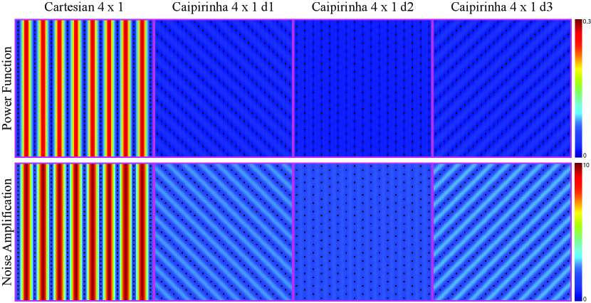
Figure 6: Sampling pattern, combined power function, and local noise amplification for Cartesian $4\times 1$ and three different CAIPIRINHA sampling patterns with different shifts. Only a part of the full grid is shown.

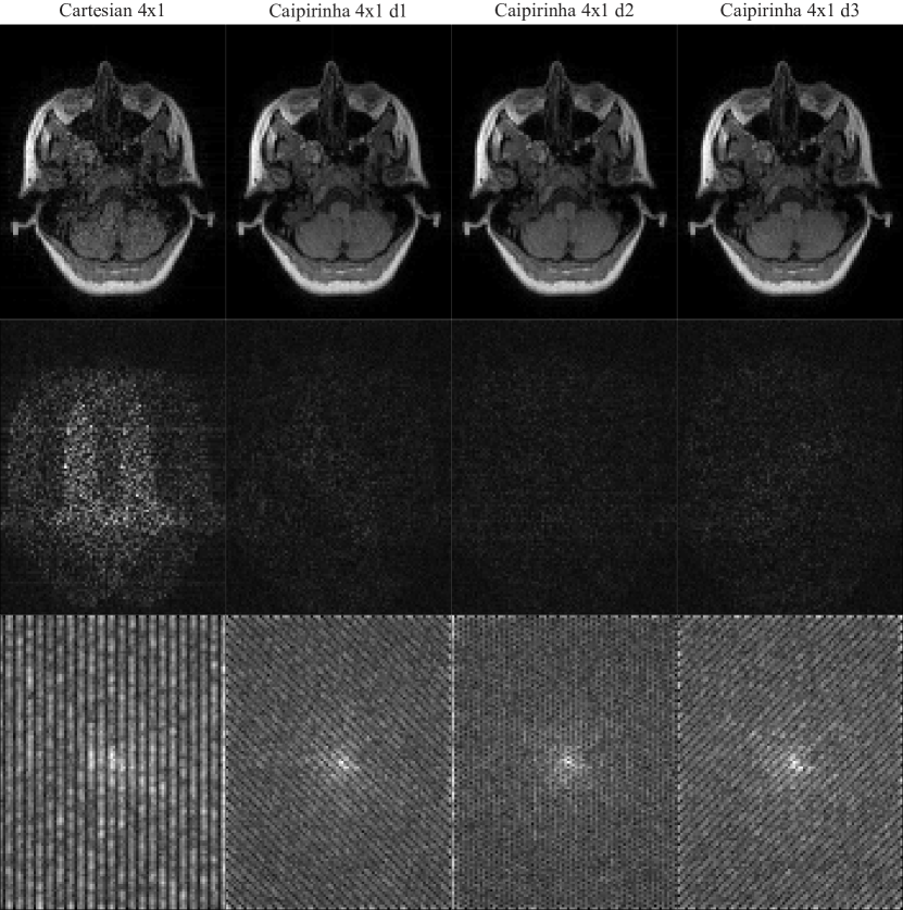
Figure 7: Images reconstructed from noisy data (top) and corresponding error maps in the image domain (middle) and k-space domain (bottom) for Cartesian $4\times 1$ sampling and CAIPIRINHA with different shifts. The k-space maps have been raised to a power of $1/3$ for improved visualization.

The differences between Cartesian $4\times 1$ and the CAIPIRINHA patterns for the power function and Frobenius norm of the cardinal functions are shown in Figure 6. Essentially distributing the undersampling in both phase-encoding dimensions, all CAIPIRINHA patterns show much lower values for both functions than the Cartesian $4\times 1$ pattern. The CAIPIRINHA pattern with a shift of two performs slightly better with respect to noise amplification than the two others. The predictions are confirmed in the reconstructions from noisy data and corresponding error maps in image and k-space domain (Fig. 7).

In summary, the results confirm the intuition that Cartesian $2\times 2$ and Poisson-disc sampling yield better k-space interpolation and less noise amplification and consequently better image reconstruction than uniform random sampling. Poisson-disc sampling is only slightly worse than Cartesian $2\times 2$ sampling. Also as expected, Cartesian $4\times 1$ performs worse than Cartesian $2\times 2$ and all CAIPIRINHA $4\times 1$ sampling patterns. The new proposed metrics can predict local reconstruction errors in k-space for different sampling patterns.

4 Discussion

4.1 Parallel Imaging as Approximation in an RKHS

In this work, it has been shown that the space of ideal multi-channel k-space signals in MRI is an RKHS. As such, it is completely characterized by its kernel, which can be derived from the spatial sensitivity profiles of the receive coils. Based on this result, the connection to approximation theory is fully developed. The interpolation formula (Eq. 14) allows optimal reconstruction from samples at arbitrary locations in k-space, i.e. it provides a solution to the reconstruction problem of Cartesian and non-Cartesian parallel MRI. If samples are acquired on arbitrary positions, the kernel (Eq. 2.3) can be evaluated by non-uniform FFT techniques [10, 11, 13]. It has to be acknowledged that solving Equation 13 is far too expensive for practical applications. In fact, image reconstruction using iterative optimization of Equation 1 still seems to be the best approach due to its efficiency and flexibility. This does not mean that Equation 13 is of purely theoretical interest. While the present study focussed on numerical exactness, practical algorithms such as GRAPPA [3] and PARS [19] can be understood as a local approximation of this formula. Valuable insights can also be expected by analyzing other existing methods in this framework. For example, the calibration-consistency condition $Wx=x$ used in SPIRiT is a discrete local version of the reproducing property (Eq. 7). On the other hand, methods which use a nonlinear model to jointly estimate image content and coil sensitivities [42, 43], or use non-linear regularization terms can not directly be addressed.

4.2 Error Bounds

Previous work in parallel imaging uses g-factor maps to quantify noise behaviour in the image domain. These maps can be calculated analytically for periodic sampling patterns for SENSE [2] and GRAPPA [35]. For arbitrary sampling patterns g-factor maps can be computed using Monte-Carlo methods based on full reconstructions [44]. While the g-factor map is a valuable tool to assess noise in the reconstructed image, it does not offer any direct insights into the source of these errors in k-space.

The present work describes new tools to study approximation error and noise amplification in k-space. The power functions can be used to predict local approximation errors for different sampling patterns, and the noise behaviour can be analyzed using the Frobenius norm of the cardinal functions. This is demonstrated in several experimental examples. CAIPIRINHA patterns have been developed to improve parallel imaging in 3D MRI by shifting samples in each k-space row by a different amount. Using the power function, it was directly confirmed that this leads to smaller errors bounds between samples. In the important combination of compressed sensing and parallel imaging [45, 46, 47], sampling schemes must provide incoherence while optimally exploiting the information from multiple coils. In this context, Poisson-disc sampling has been proposed as a replacement for random sampling based on the idea that the close area around a sample should not be sampled again because it is highly correlated for multiple coils and can be recovered with parallel MRI [48]. This intuitive idea could be confirmed for a specific coil array by comparing the power function for different sampling schemes. It is noteworthy that the lowest values for the power function could be achieved with Cartesian sampling. Although the power function yields useful error bounds in k-space, it is important to keep in mind that the optimal choice of the sampling scheme may depend on other factors such as the structure of the aliasing in the image domain. A limitation of the present work is that only a linear reconstruction is considered, while compressed sensing is a non-linear method. In compressed sensing, random or Poisson-disc sampling is used to produce incoherent aliasing which can then be removed using sparsity constraints to achieve higher acceleration.

4.3 Extensions

In the present study, it was assumed that all channel are always sampled simultaneously. While this is a reasonable assumption for data acquisition in MRI, the mathematical theory does not impose this limitation. In fact, relaxing this condition allows some interesting extensions. For example, by augmenting the RKHS with a uniformly sensitive “coil” that collects no data [49], it is possible to bound point-wise approximation errors of the Fourier transform of the single underlying image, ultimately the quantity of interest. Another possible application is the evaluation of the individual contribution of samples from different coils, which might be useful in the context of coil selection and array compression schemes [50, 51, 52]. An interesting application of the new metrics derived in this work could be the automatic design of optimal sampling patterns. For example, such techniques have previously been developed based on a greedy approach using an analytical formula for the global noise error [53], using simulated annealing using an approximate reconstruction [54], or Bayesian experimental design [55]. In these applications, localized error metrics in k-space could be used to guide the automatic selection of new sample points.

In this work, regularization has been used only at a small level to stabilize the numerical computations with the ill-conditioned kernel matrix. A higher regularization parameter can be used to optimize the trade-off between noise amplification and approximation error. This will be studied in a future work.

Coil sensitivities have to be estimated from experimental data, for example using ESPIRiT. One important result of ESPIRiT is that in some cases of corruption the coil sensitivities can not be determined uniquely. In this case, multiple sets of maps $c^{l}_{j}$ for $l=1\dots L$ appear, which have to be used simultaneously in the reconstruction. In the framework described here, this corresponds to kernels of the form

$$K_{ij}(\boldsymbol{x},\boldsymbol{y}) :=\int_{\Omega}d\boldsymbol{r}\,e^{-2\pi\sqrt{-1}(\boldsymbol{x}-\boldsymbol{y})\cdot\boldsymbol{r}}\sum_{l=1}^{L}c^{l}_{i}(\boldsymbol{r})\overline{c^{l}_{j}(\boldsymbol{r})}\leavevmode\nobreak\ .$$ (29)

Finally, it should be noted that the framework of approximation theory is very general and can be applied to completely different encoding schemes, e.g. non-linear gradient fields or multi-slice excitation [56, 57].

5 Conclusion

In the present work, parallel MRI has been formulated as an approximation of vector-valued functions in a RKHS. This space can be completely characterized by a kernel derived from the sensitivities of the receive coils. The new formulation provides a sound mathematical framework for understanding the reconstruction process and sample selection, which has been demonstrated by experimental examples comparing Cartesian, Poisson-disc, and random sampling.

6 Acknowledgements

The authors thank Robert Schaback for helpful discussions. This study was supported by NIH grants P41RR009784 and R01EB009690, American Heart Association 12BGIA9660006, Sloan Research Fellowship, GE Healthcare, and a National Science Foundation Graduate Research Fellowship.

7 Appendix

7.1 Notation

Important symbols are listed in Table 1. Bold quantities denote vectors or vector-valued functions. An upper subscript denotes a relationship to another quantity, e.g. $\boldsymbol{K}^{\boldsymbol{x},i}$ is the representer of evaluation at k-space position $\boldsymbol{x}$ for channel $i$. Lower subscripts always denote discrete indices which select a component of a vector-valued function or an element out of a set. For example, the representer $\boldsymbol{K}^{\boldsymbol{x},i}$ itself is a vector-valued function, which can be evaluated at a specific sample position $\boldsymbol{y}_{l}\in S$ and subscripted to obtain the component for a specific channel $j$, which could then be written as $K^{\boldsymbol{x},i}_{j}(\boldsymbol{y}_{l})$.

7.2 Interpolation

The interpolation formula given in Equation 14 computes the projection $\boldsymbol{f}^{\parallel}$ of any function $\boldsymbol{f}\in H$ onto $H_{S}$ from its samples $\boldsymbol{f}(\boldsymbol{x}_{k})$ with $\boldsymbol{x}_{k}\in S$. From the reproducing property (Eq. 7) and the definition of $H_{S}$ follows that $\boldsymbol{f}^{\perp}({S})=\{0\}$. $\boldsymbol{f}^{\parallel}\in H_{S}$ can be interpolated exactly. This can be shown by expressing an arbitrary function $\boldsymbol{f}^{\parallel}\in H_{S}$ by its samples $\boldsymbol{f}^{\parallel}(\boldsymbol{x}_{k})$ at $\boldsymbol{x}_{k}\in S$:

$$\boldsymbol{f}^{\parallel}(\boldsymbol{x}) =\sum_{l=1}^{|S|}\sum_{j=1}^{N}a_{\boldsymbol{x}_{l},j}\boldsymbol{K}^{\boldsymbol{x}_{l},j}(\boldsymbol{x})$$ (30)

$$=\sum_{l=1}^{|S|}\sum_{j=1}^{N}a_{\boldsymbol{x}_{l},j}\sum_{k}^{|S|}\sum_{i=1}^{N}K_{ij}(\boldsymbol{x}_{k},\boldsymbol{x}_{l})\boldsymbol{u}^{k,i}(\boldsymbol{x})$$ (31)

$$=\sum_{k=1}^{|S|}\sum_{i=1}^{N}\sum_{l=1}^{|S|}\sum_{j=1}^{N}a_{\boldsymbol{x}_{l},j}K_{ij}(\boldsymbol{x}_{k},\boldsymbol{x}_{l})\boldsymbol{u}^{k,i}(\boldsymbol{x})$$ (32)

$$=\sum_{k=1}^{|S|}\sum_{i=1}^{N}f^{\parallel}_{i}(\boldsymbol{x}_{k})\boldsymbol{u}^{k,i}(\boldsymbol{x})$$ (33)

7.3 Error Bounds

For functions in $H$, an point-wise error bound can be computed:

$$e_{n}(\boldsymbol{x}) =|\boldsymbol{f}_{n}(\boldsymbol{x})-\boldsymbol{\hat{f}}_{n}(\boldsymbol{x})|$$ (34)

$$=\bigg{|}\boldsymbol{f}_{n}(\boldsymbol{x})-\sum_{k=1}^{|S|}\sum_{i=1}^{N}f_{i}(\boldsymbol{x}_{k})u^{k,i}_{n}(\boldsymbol{x})\bigg{|}$$ (35)

$$=\bigg{|}\Big{\langle}\boldsymbol{K}^{\boldsymbol{x},n}-\sum_{k=1}^{|S|}\sum_{i=1}^{N}\boldsymbol{K}^{\boldsymbol{x}_{k},i}u^{k,i}_{n}(\boldsymbol{x}),\boldsymbol{f}\Big{\rangle}_{H}\bigg{|}$$ (36)

$$\leq\|\boldsymbol{f}\|_{H}\underbrace{\bigg{\|}\boldsymbol{K}^{\boldsymbol{x},n}-\sum_{k=1}^{|S|}\sum_{i=1}^{N}\boldsymbol{K}^{\boldsymbol{x}_{k},i}u^{k,i}_{n}(\boldsymbol{x})\bigg{\|}_{H}}_{P_{n}(\boldsymbol{x})}$$ (37)

Where $P_{n}$ is the $n$-th component of the power function. Using the reproducing property on the kernel itself $\left<\boldsymbol{K}^{\boldsymbol{x},i},\boldsymbol{K}^{\boldsymbol{y},j}\right>_{H}=K_{ij}(\boldsymbol{x},\boldsymbol{y})$, it can be expressed as:

$$P_{n}^{2}(\boldsymbol{x})=K_{nn}(\boldsymbol{x},\boldsymbol{x})-2{\mathcal{R}e}\sum_{k=1}^{|S|}\sum_{i=1}^{N}K_{in}(\boldsymbol{x}_{k},\boldsymbol{x})u_{n}^{ik}(\boldsymbol{x})$$ (38)

$$\qquad+\sum_{l=1}^{|S|}\sum_{k=1}^{|S|}\sum_{i=1}^{N}\sum_{j=1}^{N}K_{ij}(\boldsymbol{x}_{k},\boldsymbol{x}_{l})u_{n}^{ik}(\boldsymbol{x})\overline{u_{n}^{jl}(\boldsymbol{x})}$$ (39)

For an unregularized least-squares reconstruction the interpolation error is orthogonal to the interpolant, i.e. $<\boldsymbol{f}-\hat{\boldsymbol{f}},\hat{\boldsymbol{f}}>_{H}=0$. In this case, the power function can be simplified to:

$$P_{n}^{2}(\boldsymbol{x})=K_{nn}(\boldsymbol{x},\boldsymbol{x})-\sum_{l=1}^{|S|}\sum_{j=1}^{N}K_{nj}(\boldsymbol{x},\boldsymbol{x}_{l})\overline{u_{n}^{jl}(\boldsymbol{x})}$$ (40)

References

- [1] D. K. Sodickson and W. J. Manning. Simultaneous acquisition of spatial harmonics (SMASH): Fast imaging with radiofrequency coil arrays. Magn Reson Med, 38:591–603, 1997.
- [2] K. P. Pruessmann, M. Weiger, M. B. Scheidegger, and P. Boesiger. SENSE: Sensitivity encoding for fast MRI. Magn Reson Med, 42:952–962, 1999.
- [3] M. A. Griswold, P. M. Jakob, R. M. Heidemann, M. Nittka, V. Jellus, J. Wang, B. Kiefer, and A. Haase. Generalized autocalibrating partially parallel acquisitions (GRAPPA). Magn Reson Med, 47:1202–10, 2002.
- [4] J. B. Ra and C. Y. Rim. Fast imaging using subencoding data sets from multiple detectors. Magn Reson Med, 30:142–145, 1993.
- [5] K. P. Pruessmann, M. Weiger, P. Börnert, and P. Boesiger. Advances in sensitivity encoding with arbitrary k-space trajectories. Magn Reson Med, 46:638–651, 2001.
- [6] S. A. R. Kannengiesser, A. R. Brenner, and T. G. Noll. Accelerated image reconstruction for sensitivity encoded imaging with arbitrary k-space trajectories. In Proceedings of the 8th ISMRM Annual Meeting, page 155, Denver, 2000.
- [7] D. K. Sodickson and C. A. McKenzie. A generalized approach to parallel magnetic resonance imaging. Med Phys, 28:1629–1643, 2001.
- [8] M. Bertero, C. De Mol, and E. R. Pike. Linear inverse problems with discrete data. i. general formulation and singular system analysis. Inverse Problems, 1:301–330, 1985.
- [9] R. Van de Walle, H. H. Barrett, K. J. Myers, M. I. Altbach, B. Desplanques, A. F. Gmitro, J. Cornelis, and I. Lemahieu. Reconstruction of mr images from data acquired on a general nonregular grid by pseudoinverse calculation. IEEE Trans Med Imaging, 19:1160–1167, 2000.
- [10] J. D. O’Sullivan. A fast sinc function gridding algorithm for Fourier inversion in computer tomography. IEEE Trans Med Imaging, 4:200–207, 1985.
- [11] J. I. Jackson, C.H. Meyer, D.G. Nishimura, and A. Macovski. Selection of a convolution function for Fourier inversion using gridding. IEEE Trans Med Imaging, 3:473–478, 1991.
- [12] J. A. Fessler and B. P. Sutton. Nonuniform fast Fourier transforms using min-max interpolation. IEEE Trans Med Imaging, 51:560–574, 2003.
- [13] P. J. Beatty, D. G. Nishimura, and J. M. Pauly. Rapid gridding reconstruction with a minimal oversampling ratio. IEEE Trans Med Imaging, 24:799–808, 2005.
- [14] M. Uecker, S. Zhang, D. Voit, K.-D. Merboldt, and J. Frahm. Real time MRI: Recent advances using radial FLASH. Imaging in Medicine, 4:461–476, 2012.
- [15] N. Seiberlich, P. Ehses, J. Duerk, R. Gilkeson, and M. Griswold. Improved radial GRAPPA calibration for real-time free-breathing cardiac imaging. Magn Reson Med, 65:492–505, 2011.
- [16] B. Xu, P. Spincemaille, G. Chen, M. Agrawal, T. D. Nguyen, M. R. Prince, and Y. Wang. Fast 3d contrast enhanced MRI of the liver using temporal resolution acceleration with constrained evolution reconstruction. Magn Reson Med, 69:370–381, 2013.
- [17] L. Feng, R. Grimm, K. T. Block, H. Chandarana, S. Kim, J. Xu, L. Axel, D. K. Sodickon, and R. Otazo. Golden-angle radial sparse parallel MRI: Combination of compressed sensing, parallel imaging, and golden-angle radial sampling for fast and flexible dynamic volumetric MRI. Magn Reson Med, 2013. Epub, doi: 10.1002/mrm.24980.
- [18] C. A. McKenzie, M. A. Ohliger, E. N. Yeh, M. D. Price, and D. K. Sodickson. Coil-by-coil image reconstruction with SMASH. Magn Reson Med, 46:619–623, 2001.
- [19] E. N. Yeh, C. A. McKenzie, M. A. Ohliger, and D. K. Sodickson. Parallel magnetic resonance imaging with adaptive radius in k-space (PARS): constrained image reconstruction using k-space locality in radiofrequency coil encoded data. Magn Reson Med, 53:1383–1392, 2005.
- [20] R. M. Heidemann, M. A. Griswold, N. Seiberlich, G. Krüger, S. A. R. Kannengiesser, B. Kiefer, G. Wiggins, L. L. Wald, and P. Jakob. Direct parallel image reconstructions for spiral trajectories using GRAPPA. Magn Reson Med, 56:317–326, 2006.
- [21] A. A. Samsonov, W. F. Block, A. Arunachalam, and A. S. Field. Advances in locally constrained k-space-based parallel MRI. Magn Reson Med, 55:431–438, 2006.
- [22] P. J. Beatty, B. A. Hargreaves, P. T. Gurney, and D. G. Nishimura. Method for non-cartesian parallel imaging reconstruction with improved calibration. In Proceedings of the 9th ISMRM Annual Meeting, Berlin, 2007.
- [23] F. Huang, S. Vijayakumar, Y. Li, S. Hertel, S. Reza, and G. R. Duensing. Self-calibration method for radial GRAPPA/k-t GRAPPA. Magn Reson Med, 57:1075–1085, 2007.
- [24] N. Seiberlich, F. A. Breuer, M. Blaimer, K. Barkauskas, P. M. Jakob, and M. A. Griswold. Non-Cartesian data reconstruction using GRAPPA operator gridding (GROG). Magn Reson Med, 58:1257–1265, 2007.
- [25] N. Seiberlich, F. Breuer, R. Heidemann, M. Blaimer, M. Griswold, and P. Jakob. Reconstruction of undersampled non-Cartesian data sets using pseudo-Cartesian GRAPPA in conjunction with GROG. Magn Reson Med, 59:1127–1137, 2008.
- [26] N. C. F. Codella, P. Spincemaille, M. Prince, and Y. Wang. A radial self-calibrated (RASCAL) generalized autocalibrating partially parallel acquisition (GRAPPA) method using weight interpolation. NMR Biomed, 24:844–854, 2011.
- [27] M. Uecker, P. Lai, M. J. Murphy, P. Virtue, M. Elad, J. M. Pauly, S. S. Vasanawala, and M. Lustig. ESPIRiT – an eigenvalue approach to auto-calibrating parallel MRI: Where SENSE meets GRAPPA. Magn Reson Med, 71:990–1001, 2014.
- [28] N. Aronszajn. Theory of reproducing kernels. Trans Amer Math Soc, 68:337–404, 1950.
- [29] H. Wendland. Scattered Data Approximation. Cambridge University Press, 2005.
- [30] K. A. Heberlein and X. Hu. Kriging and GRAPPA: a new perspective on parallel imaging reconstruction. In Proceedings of the 14th Annual Meeting of the ISMRM, page 2465, Seattle, 2006.
- [31] Y. Chang, D. Liang, and L. Ying. Nonlinear GRAPPA: A kernel approach to parallel MRI reconstruction. Magn Reson Med, 68:730–740, 2012.
- [32] Z. Wu and R. Schaback. Local error estimates for radial basis function interpolation of scattered data. PIMA J Numer Anal, 13:13–27, 1993.
- [33] F. J. Narcowich and J. D. Ward. Generalized hermite interpolation via matrix-valued conditionally positive definite functions. Math Comp, 63:661–687, 1994.
- [34] E. J. Fuselier. Refined Error Estimates for Matrix-Valued Radial Basis Functions. PhD thesis, Texas A&M University, 2006.
- [35] F. A. Breuer, S. A. R. Kannengiesser, M. Blaimer, N. Seiberlich, P. M. Jakob, and M. A. Griswold. General formulation for quantitative g-factor calculation in GRAPPA reconstructions. Magn Reson Med, 62:739–746, 2009.
- [36] L. N. Trefethen. Approximation Theory and Approximation Practice. SIAM, 2013.
- [37] L. Yuan, L. Ying, D. Xu, and Z.-P. Liang. Truncation effects in SENSE reconstruction. Magnetic Resonance Imaging, 24:1311–1318, 2006.
- [38] J. Tsao, J. Sánchez, P. Boesiger, and K. P. Pruessmann. Minimum-norm reconstruction for optimal spatial response in high-resolution SENSE imaging. In Proceedings of the 11th ISMRM Annual Meeting, page 0014, 2003.
- [39] J. Sánchez-González, J. Tsao, U. Dydak, M. Desco, P. Boesiger, and K. P. Pruessmann. Minimum-norm reconstruction for sensitivity-encoded magnetic resonance spectroscopic imaging. Magn Reson Med, 55:287–295, 2006.
- [40] M. Uecker. Nonlinear Reconstruction Methods for Parallel Magnetic Resonance Imaging. PhD thesis, Georg-August-Universität Göttingen, 2009.
- [41] F. A. Breuer, M. Blaimer, M. F. Mueller, N. Seiberlich, R. M. Heidemann, M. A. Griswold, and P. M. Jakob. Controlled aliasing in volumetric parallel imaging (2D CAIPIRINHA). Magn Reson Med, 55:549–556, 2006.
- [42] L. Ying and J. Sheng. Joint image reconstruction and sensitivity estimation in sense (JSENSE). Magn Reson Med, 57:1196–1202, 2007.
- [43] M. Uecker, T. Hohage, K. T. Block, and J. Frahm. Image reconstruction by regularized nonlinear inversion – joint estimation of coil sensitivities and image content. Magn Reson Med, 60:674–682, 2008.
- [44] P. M. Robson, A. K. Grant, A. J. Madhuranthakam, R. Lattanzi, D. K. Sodickson, and C. A. McKenzie. Comprehensive quantification of signal-to-noise ratio and g-factor for image-based and k-space-based parallel imaging reconstructions. Magn Reson Med, 60:895–907, 2008.
- [45] K. T. Block, M. Uecker, and J. Frahm. Undersampled radial MRI with multiple coils. Iterative image reconstruction using a total variation constraint. Magn Reson Med, 57:1086–1098, 2007.
- [46] B. Liu, K. King, M. Steckner, J. Xie, J. Sheng, and L. Ying. Regularized sensitivity encoding (SENSE) reconstruction using bregman iterations. Magn Reson Med, 61:145–152, 2009.
- [47] M. Lustig and J. M. Pauly. SPIRiT: Iterative self-consistent parallel imaging reconstruction from arbitrary k-space. Magn Reson Med, 64:457–471, 2010.
- [48] S. S. Vasanawala, M. J. Murphy, M. T. Alley, P. Lai, K. Keutzer, J. M. Pauly, and M. Lustig. Practical parallel imaging compressed sensing mri: Summary of two years of experience in accelerating body mri of pediatric patients. In Biomedical Imaging: From Nano to Macro, 2011 IEEE International Symposium on, pages 1039–1043, Chicago, 2011.
- [49] P. J. Beatty, W. Sun, and A. C. Brau. Direct virtual coil (dvc) reconstruction for data-driven parallel imaging. In Proceedings of the 16th Annual Meeting of the ISMRM, page 8, Toronto, 2008.
- [50] M. Buehrer, K. P. Pruessmann, P. Boesiger, and S. Kozerke. Array compression for MRI with large coil arrays. Magn Reson Med, 57:1131–1139, 2007.
- [51] F. Huang, S. Vijayakumar, Y. Li, S. Hertel, and G. R. Duensing. A software channel compression technique for faster reconstruction with many channels. Magn Reson Imaging, 26:133–141, 2008.
- [52] T. Zhang, J. M. Pauly, S. S. Vasanawala, and M. Lustig. Coil compression for accelerated imaging with Cartesian sampling. Magn Reson Med, 69:571–582, 2013.
- [53] D. Xu, M. Jacob, and Z. P. Liang. Optimal sampling of k-space on Cartesian grids for parallel MR imaging. In Proceedings of the 13th ISMRM Annual Meeting, page 2450, 2005.
- [54] E. Gong, F. Huang, K. Ying, X. Liu, and G. R. Duensing. An efficient scheme of trajectory optimization for both parallel imaging and compressed sensing. In Proceedings of the 21th ISMRM Annual Meeting, page 2367, 2013.
- [55] M. Seeger, H. Nickisch, R. Pohmann, and B. Schölkopf. Optimization of k-space trajectories for compressed sensing by bayesian experimental design. Magn Reson Med, pages 116–126, 2010.
- [56] J. Hennig, A. M. Welz, G. Schultz, J. Korvink, Z. Liu, O. Speck, and M. Zaitsev. Parallel imaging in non-bijective, curvilinear magnetic field gradients: a concept study. MAGMA, 21:5–14, 2008.
- [57] D. J. Larkman, J. V. Hajnal, A. H. Herlihy, G. A. Coutts, I. R. Young, and G. Ehnholm. Use of multicoil arrays for separation of signal from multiple slices simultaneously excited. J Magn Reson Imaging, 13:313–317, 2001.