Primordial non-Gaussianity in the bispectra of large-scale structure

Abstract

The statistics of large-scale structure in the Universe can be used to probe non-Gaussianity of the primordial density field, complementary to existing constraints from the cosmic microwave background. In particular, the scale dependence of halo bias, which affects the halo distribution at large scales, represents a promising tool for analyzing primordial non-Gaussianity of local form. Future observations, for example, may be able to constrain the trispectrum parameter $g_{\rm NL}$ that is difficult to study and constrain using the CMB alone. We investigate how galaxy and matter bispectra can distinguish between the two non-Gaussian parameters $f_{\rm NL}$ and $g_{\rm NL}$, whose effects give nearly degenerate contributions to the power spectra. We use a generalization of the univariate bias approach, making the hypothesis that the number density of halos forming at a given position is a function of the local matter density contrast and of its local higher-order statistics. Using this approach, we calculate the halo-matter bispectra and analyze their properties. We determine a connection between the sign of the halo bispectrum on large scales and the parameter $g_{\rm NL}$. We also construct a combination of halo and matter bispectra that is sensitive to $f_{\rm NL}$, with little contamination from $g_{\rm NL}$. We study both the case of single and multiple sources to the primordial gravitational potential, discussing how to extend the concept of stochastic halo bias to the case of bispectra. We use a specific halo mass-function to calculate numerically the bispectra in appropriate squeezed limits, confirming our theoretical findings.

I Introduction

The intrinsic non-Gaussianity of primordial curvature perturbations is a valuable tool to distinguish among different models for the origin of structure in the very early universe Bartolo:2004if . Even if the primordial curvature perturbation has a Gaussian distribution, the initial density perturbation is non-Gaussian due to the non-linearity of the Einstein field equations Verde:2009hy ; Bartolo:2010rw ; Bruni:2013qta . Non-Gaussianity (nG) may be characterized by a variety of different parameters, which control the departure of the underlying probability distribution function (pdf) of primordial fluctuations from a purely Gaussian distribution. These parameters can be related to the amplitude of connected $n$-point ($n$-pt) correlation functions of primordial curvature fluctuations that vanish for $n>2$ in the Gaussian case. The connected $n$-pt functions may be scale- and shape-dependent, in a manner determined by the particular model that generates them.

In this work, we will focus on the so-called local shape of nG, in which the primordial gravitational potential in coordinate space can be expressed as an expansion in powers of one or more Gaussian random fields that determine the primordial density fluctuations. In this case 3-pt functions of curvature fluctuations are determined by a parameter, $f_{\rm NL}$, that at lowest order in a perturbative expansion characterizes the skewness of the pdf of primordial fluctuations. 4pt functions are determined by parameters, $g_{\rm NL}$ and $\tau_{\rm NL}$, controlling the kurtosis of the pdf at lowest order in perturbations. The recent release of Planck data allows one to set the best constraints yet on primordial non-Gaussian parameters from cosmic microwave background (CMB) data alone Ade:2013ktc . The quantity $f_{\rm NL}$ (local) is now constrained to be $|f_{\rm NL}|\leq 15$ at 2$\sigma$ level, while $\tau_{\rm NL}\leq 2800$; an analysis of the constraints on $g_{\rm NL}$ local from Planck data has yet to be completed, but the forecast $1\sigma$ error bar with Planck data has been estimated to be $\sigma_{g_{\rm NL}}=6.7\times 10^{4}$ by Sekiguchi:2013hza and $\sigma_{g_{\rm NL}}=1.3\times 10^{5}$ by Smidt:2010ra . It may be unlikely that we live in a universe with a large hierarchy between $f_{\rm NL}$ and $g_{\rm NL}$ local Nurmi:2013xv , but this possibility cannot be excluded a priori and there are theoretical models able to predict this pattern (see for example Byrnes:2009qy or the discussion in Suyama:2013nva ). Since $f_{\rm NL}$ and $g_{\rm NL}$ control distinct features of the pdf (skewness and kurtosis) it is very important to have the best observational constraints on each of them. Complementary observables have to be considered to set more stringent bounds on non-Gaussian parameters, in particular on $g_{\rm NL}$, and one possibility is to use the statistics of large-scale structure.

Pioneering papers by Dalal et al Dalal:2007cu , Slosar et al Slosar:2008hx , Matarrese et al Matarrese:2008nc , Afshordi and Tolley Afshordi:2008ru highlighted an interesting feature of primordial nG of local shape: it introduces a specific correlation between modes of different wavelengths which leads to a characteristic scale dependence of the halo bias. Much work has been done so far to explore this interesting topic (see Gong:2011gx ; Desjacques:2008vf ; Desjacques:2011jb ; Desjacques:2011mq and Desjacques:2010jw ; Verde:2010wp for reviews). However it turns out to be challenging to disentangle the contributions from different non-Gaussian parameters using only halo and matter power spectra, since the characteristic scale dependence of the bias is primarily sensitive to a particular combination of the $f_{\rm NL}$ and $g_{\rm NL}$ parameters Desjacques:2009jb ; Roth:2012yy . Mild corrections associated with the red-shift dependence of the halo mass function have been used to set the first LSS constraints on $g_{\rm NL}$ in Giannantonio:2013uqa , but it is difficult to convincingly distinguish the effect of $f_{\rm NL}$ from that of $g_{\rm NL}$ using only galaxy power spectra. Independent constraints on $f_{\rm NL}$ from CMB are useful, but not conclusive because $f_{\rm NL}$ could be characterized by a significant scale dependence LoVerde:2007ri ; Byrnes:2010ft , that makes its value probed at LSS scales different with respect to the one tested at CMB scales.

A promising method that may break the degeneracy between $f_{\rm NL}$ and $g_{\rm NL}$ is to study the bispectra of halo and matter densities, which are sensitive to a non-linear bias parameter that depends specifically on $g_{\rm NL}$, and allows us to break the aforementioned degeneracy. Jeong and Komatsu Jeong:2009vd (see also Sefusatti:2009qh ) were the first among various groups to include the scale dependence of halo bias when studying bispectra, by considering the non-linear evolution of the halo overdensity in a local, univariate bias expansion, where the halo abundance is taken to be a function of the local density. They have shown that galaxy bispectra are sensitive to non-Gaussian parameters beyond $f_{\rm NL}$, as confirmed by $N$-body simulations Nishimichi:2009fs ; Sefusatti:2011gt . In this work, we elaborate on this subject. We will show that halo and matter bispectra have interesting qualitative features that may allow us to distinguish between the effects of different primordial nG parameters.

We implement a peak-background split method within a barrier crossing approach to re-derive in part the results of Jeong:2009vd in a physically transparent way, and to extend their analysis in various directions with the main aim of understanding how the parameters $f_{\rm NL}$ and $g_{\rm NL}$ can be possibly distinguished when analyzing the statistics of halo and matter bispectra.

In order to focus only on the consequences of primordial non-Gaussian initial conditions on the properties of bispectra, we will not include the effects of non-linear gravitational clustering in our analysis; that is, we work in Lagrangian space and linearly transform to Eulerian space. We also neglect non-linearity in the halo mass function, i.e., non-linear local bias, which implies that any non-vanishing bispectra will be solely due to primordial nG.

Our work contains several results, and we present these in a modular way to render the paper easier to read. We begin with some theoretical sections discussing how to implement the peak-background split and barrier crossing approaches to determine concise analytical expressions for halo and matter bispectra, when the gravitational potential is a function of either single or multiple sources (e.g., due to fluctuations of single or multiple fields during inflation in the very early universe). Our formulae are obtained by applying to bispectra the methods developed in Baumann:2012bc for power spectra. See also Scoccimarro:2011pz for an interesting paper discussing how to implement the peak background splitting approach to bispectra.

We use a generalization of the univariate bias approach, making the hypothesis that the local number of halos forming at a given position is a function of the matter contrast, and of its local correlation functions evaluated at that position. This is an alternative to the bivariate approach Giannantonio:2009ak where the halo abundance is assumed to be a function of both the density field and the gravitational potential. In practice, the physical effect of long-wavelength modes of the potential is to modulate the small-scale variance of the density field in local models of nG. Our extended univariate approach is physically transparent, and allows us to recover some of the results of the bivariate approach, in appropriate limits. In addition we can include local variations of effective non-Gaussianity parameters on halo abundance Byrnes:2011ri . The resulting bispectra contain several contributions scaling with different powers of the scale $k$, weighted by coefficients depending on primordial non-Gaussian parameters. In the limit of large scales, in which analytic expressions for the transfer functions can be derived, we will discuss how bispectra have qualitative features that make it possible, at least in principle, to distinguish the effects of $f_{\rm NL}$ and $g_{\rm NL}$. For example, by studying the properties of the bispectra as a function of the scale, we determine a connection between the sign of the halo bispectrum and nG parameters, in particular the value of $g_{\rm NL}$. Moreover, we show that there exists a combination of halo and matter bispectra that is sensitive to $f_{\rm NL}$ only, allowing us to probe $f_{\rm NL}$ without contaminations from $g_{\rm NL}$.

We then extend all these results, obtained in the case of a single source for the primordial gravitational potential, to a two-field example that allows us to understand how multiple sources contribute to galaxy bispectra. In Tseliakhovich:2010kf ; Baumann:2012bc it was pointed out that if multiple fields source the primordial gravitational potential, then halo overdensities need not be fully correlated with matter overdensities. We show that a combination of halo and matter power spectra is particularly convenient for studying the phenomenon of stochastic halo bias. Our analysis enable us to extend the concept of stochastic halo bias in the presence of primordial nG to the cases of both power spectra and bispectra, including the effect of $g_{\rm NL}$. The fact that this stochastic bias is non-vanishing can be interpreted in terms of inequalities satisfied by primordial non-Gaussian parameters, and these provide information on the number of fundamental fields sourcing nG. We determine a new combination of halo and matter bispectra whose value can be used to distinguish the effect of single and multiple sources on the primordial gravitational potential, and discuss its physical interpretation.

In the second part of our work, we apply our theoretical findings to a systematic numerical analysis of bispectra in appropriate squeezed limits, by using Press-Schechter halo mass functions supplemented by non-Gaussian corrections controlled by an Edgeworth expansion. This discussion enables us to apply our results to scales and redshifts that can be probed in present or future surveys. By plotting the resulting halo bispectra, we explore the different roles played by $f_{\rm NL}$ and $g_{\rm NL}$. The numerical analysis confirms our analytical results. We show that qualitative features of the profiles of halo and matter bispectra as a function of the scale are sensitive to different nG parameters, possibly allowing us to test them individually. These results clearly demonstrate how galaxy bispectra have features that could distinguish between different non-Gaussian parameters, in a way that is not possible by studying only the scale dependence of galaxy bias in power spectra of halos and matter.

We conclude with a discussion on possible improvements and future directions for our investigation.

II The statistics of dark matter halos

We start with an introductory section outlining the ideas that we will use to treat the statistics of dark matter halos Baumann:2012bc . The primordial gravitational potential $\Phi$ is related to the linearly evolved matter density contrast $\delta$ in terms of the Poisson equation in Fourier space

$$\delta_{\vec{k}}(z)\,=\,\bar{\alpha}(k,\,z)\,\Phi_{\vec{k}}\,,$$ (1)

where

$$\bar{\alpha}(k,z)\,=\,\frac{2\,k^{2}\,T(k)\,D(z)}{3\,\Omega_{m}\,H_{0}^{2}}\,.$$ (2)

$T(k)$ is the matter transfer function normalized such that $T(k)\to 1$ at large scales $k\to 0$. $D(z)$ is the linear growth factor, as a function of redshift $z$. It is normalized such that $D(z)\,=\,(1+z)^{-1}$ in matter domination. At very large scales $k\ll 1$, the function $\bar{\alpha}$ is proportional to $k^{2}$ Bernardeau:2001qr :

$$\bar{\alpha}(k,z)\simeq\frac{2k^{2}D(z)}{3\Omega_{m}H_{0}^{2}}=\alpha_{0}(z)k^{2}\quad\text{where}\quad\alpha_{0}(z)\simeq 2.16\cdot 10^{7}\,\left(\frac{0.277D(z)}{\Omega_{m}}\right)\,\left(\frac{\text{Mpc}}{h}\right)^{2}\,.$$ (3)

This asymptotic behavior will be useful to get analytic results in the discussion of Section III.2.1. To render the formulae less cumbersome, from now on we will suppress the $z$ dependence.

The field $\delta_{M}(\vec{x})$ denotes the linear density contrast smoothed with a top-hat filter of radius $R_{M}\,=\,(3M/4\pi\bar{\rho}_{m})^{1/3}$ where $M$ is the halo mass, and $\bar{\rho}_{m}$ the background matter density. In Fourier space, we write

$$\delta_{M}(\vec{k})\,=\,W_{M}(k)\,\delta_{\vec{k}}$$ (4)

with $W_{M}$ the Fourier transform of top-hat filter:

$$W_{M}(k)\,=\,3\,\frac{\sin{(kR_{M})}-kR_{M}\,\cos{(kR_{M})}}{\left(k\,R_{M}\right)^{3}}\,.$$ (5)

We also define $\sigma_{M}\equiv\langle\delta_{M}^{2}\rangle^{\frac{1}{2}}$ and $\alpha(k)\,=\,W_{M}(k)\bar{\alpha}(k)$. At large scales $W_{M}(k\to 0)\,=\,1$.

In what follows, we will investigate the statistical properties of the spatial distribution of galaxies. In the widely accepted model of galaxy formation, known as the halo model, galaxies form in the potential wells of gravitationally collapsed dark matter halos White:1977jf . The distribution of galaxies naturally follow the distribution of halos. There are various approaches to characterize their formation, and how they are distributed in space. In the barrier crossing approach, initiated by Press and Schechter Press:1973iz , halos are thought to form when the matter linear overdensity field overcomes a certain threshold $\delta_{c}$. We denote the number of halos of mass $M$ at time $t$ by $n_{h}(\vec{x},M,t)$: the Press-Schechter mass function gives the mean number density $n_{h}$ of halos as a function of the properties of the underlying linear matter overdensity field $\delta_{M}$. In the following, we will drop the dependence on $M$ and $t$ (or $z$) to simplify the notation.

In our work, we assume that $n_{h}(\vec{x})$ depends on local physics only, i.e. it is a local function of $\delta(\vec{x})$ and of its $n$-pt correlation functions

$$\left[\delta^{n}\right]_{v}(\vec{x})\,\equiv\,\int_{{k}_{i}\geq\ell^{-1}}\,\frac{d^{3}k_{1}}{(2\pi)^{3}}\dots\frac{d^{3}k_{n}}{(2\pi)^{3}}\,e^{-i\left(\vec{k}_{1}+\dots+\vec{k}_{n}\right)\,\vec{x}}\,\langle\delta_{\vec{k}_{1}}\dots\delta_{\vec{k}_{n}}\rangle$$

evaluated within a region $v\sim\ell^{3}$ around the position $\vec{x}$ (see Section III for an additional discussion on this assumption):

$$n_{h}(\vec{x})\,=\,\bar{n}_{h}(\delta(\vec{x}),\,\left[\delta^{n}\right]_{v}(\vec{x}))\,.$$ (6)

The autocorrelations $\left[\delta^{n}\right]_{v}$ depend on the primordial intrinsic nG of the fundamental fields that seed the gravitational potential $\Phi$. By measuring how the statistics of the halo displacement

$$\delta_{h}=(n_{h}-\langle n_{h}\rangle)/\langle n_{h}\rangle$$

is related to the statistics of the matter density displacement $\delta$, one can extract information about primordial nG.

The local statistics of the autocorrelations $\left[\delta^{n}\right]_{v}$ can be calculated using a heuristic but powerful method, the so called peak-background split approach Bardeen:1985tr ; Cole:1989vx . Consider a large subvolume $v\sim\ell^{3}$ of the universe containing a large number of halos. Take for concreteness a fiducial scale $\ell$, say $\ell\,\sim\,10\,{\rm Mpc}/h$, still much larger than the scale associated with halos of mass $M$. The linearized matter overdensity field $\delta(\vec{x})$ can be decomposed into a short wavelength part $\delta_{short}$ and a long wavelength background $\delta_{long}$ with respect to the scale $\ell$:

$$\delta(t,\,\vec{x})\,=\,\delta_{short}(t,\,\vec{x})+\delta_{long}(t,\,\vec{x})$$ (7)

where the short and long wavelength contributions to $\delta(t,\vec{x})$ are defined as

$$\delta_{short}(t,\,\vec{x}) = \int_{k\geq\ell^{-1}}\frac{d^{3}k}{(2\pi)^{3}}\,e^{-i\vec{k}\vec{x}}\delta_{\vec{k}}(t)\,$$ (8)

$$\delta_{long}(t,\,\vec{x}) = \int_{k\ll\ell^{-1}}\frac{d^{3}k}{(2\pi)^{3}}\,e^{-i\vec{k}\vec{x}}\delta_{\vec{k}}(t)\,.$$ (9)

The short mode $\delta_{short}$ at scales $\leq 10\,{\rm Mpc}/h$ can be considered as the source of halos within the subvolume $v$ we are focussing on. As we mentioned above, locally $n_{h}$ depends on the quantity $\delta_{short}$ within the subvolume $v$, and on its correlation functions $\left[\delta^{n}_{short}\right]_{v}$ evaluated on the same subvolume. Instead, distances larger than $100{\rm Mpc}/h$, associated with long mode $\delta_{long}$, are the scales over which we measure the statistics of halo displacements $\delta_{h}$. Within the subvolume $v$, $\delta_{long}$ acts as a smooth background density field in the linear regime. As we will discuss in the next sections, in the presence of primordial nG, $\delta_{long}$ has the important feature to modulate in a specific way the correlation functions $\left[\delta^{n}_{short}\right]_{v}$ controlling the halo displacement $\delta_{h}$. This implies that primordial nG of the gravitational potential controls the statistics of $\delta_{h}$ in such a way that it makes possible to extract from the latter unambiguous information on the former.

Hence, the barrier crossing approach and the peak-background split method allow us to analyze how primordial nG affects the statistics of LSS. The connections between the two methods have been carefully discussed in Baumann:2012bc ; Ferraro:2012bd : the statistics of $\delta_{long}$ has the effect to perturb the critical threshold that the linear part of $\delta_{short}$ has to reach to start to collapse, and it is this effect that renders the barrier crossing approach sensitive to primordial nG.

In the next sections, we will develop and apply these ideas to find quantitative results for the statistics of halo and matter displacements, both at the level of power spectrum and bispectrum, for single and multiple sources.

III The power spectrum and the bispectrum: the single source case

We start analyzing the case of single source, extending to the case of the bispectrum the results of Baumann:2012bc . We consider a large subvolume of the Universe containing many halos, over which the long mode is reasonably constant, and we denote with $\left[\cdot\right]_{\rm v}$ a spatial average over this subvolume – while $\langle\cdot\rangle$ is the spatial average over the entire universe. In this section we consider a single Gaussian field $\varphi$ as an unique source for the primordial gravitational potential. We split such a field in long and short modes with respect to a fiducial scale $\ell$:

$$\varphi\,=\,\varphi_{s}+\varphi_{L}\,.$$ (10)

This Gaussian field has zero average over the entire space $\langle\dots\rangle$, while non-zero average over the subvolume $\left[\dots\right]_{v}$, with $v\sim\ell^{3}$:

$$\langle\varphi\rangle = 0\,,$$ (11)

$$\left[\varphi\right]_{v} = \varphi_{L}\,.$$ (12)

We make a local expansion of the primordial gravitational potential up to third order in terms of the Gaussian field $\varphi$:

$$\Phi = \varphi+{f_{\rm NL}}\left(\varphi^{2}-\langle\varphi^{2}\rangle\right)+{g_{\rm NL}}\left(\varphi^{3}-3\langle\varphi^{2}\rangle\varphi\right)\,.$$ (13)

After implementing the long/short splitting we introduced in eq. (10), we get in coordinate space

$$\Phi = \varphi_{L}+{f_{\rm NL}}\left(\varphi_{L}^{2}-\langle\varphi_{L}^{2}\rangle\right)+{g_{\rm NL}}\left(\varphi_{L}^{3}-3\langle\varphi_{L}^{2}\rangle\varphi_{L}\right)$$ (14)

$$+\left(1+2f_{\rm NL}\varphi_{L}+3{g_{\rm NL}}(\varphi_{L}^{2}-\langle\varphi_{L}^{2}\rangle)\right)\varphi_{s}$$

$$+\left(f_{\rm NL}+3g_{\rm NL}\varphi_{L}\right)\left(\varphi_{s}^{2}-[\varphi_{s}^{2}]_{v}\right)$$

$$+g_{\rm NL}\left(\varphi_{s}^{3}-3[\varphi_{s}^{2}]\varphi_{s}\right)\,.$$

The previous expression demonstrates how the long wavelength mode modulates the gravitational potential. The coefficients of the different powers of $\varphi_{s}$, which control the statistics of this quantity within the subvolume $v$, receive contributions depending on the long mode $\varphi_{L}$, and this acts as a background quantity from the point of view of the subvolume $v$. In light of this, we can define the small scale effective power $\sigma^{e}\,=\,\left[\Phi^{2}\right]_{v}^{1/2}$, $f_{\rm NL}^{e}$ and $g_{\rm NL}^{e}$ as

$$\left(\sigma^{e}\right) = \left[\varphi_{s}^{2}\right]_{v}^{1/2}\,\left(1+2f_{\rm NL}\varphi_{L}+3{g_{\rm NL}}(\varphi_{L}^{2}-\langle\varphi_{L}^{2}\rangle)\right)\,,$$ (15)

$$f_{\rm NL}^{e} = f_{\rm NL}+3g_{\rm NL}\varphi_{L}\,,$$ (16)

$$g_{\rm NL}^{e} = g_{\rm NL}\,,$$ (17)

so we learn that long wavelength modes and primordial nG affect the two point statistics of the short modes, as well as the non-Gaussian parameters inside the small box. The long mode dependence of eqs (15)-(17) will be used to estimate the number of halos at a given position.

There are various approaches to the problem of quantifying how long modes contribute to the process of halo formation. The conceptually simplest one is to use an univariate approach, in which the number of halos is expressed in power series of $\delta$, the matter density contrast. An univariate approach is used by Jeong and Komatsu Jeong:2009vd . This method includes the effects of the long mode $\varphi_{L}$ of the field sourcing the gravitational potential in the halo distribution, as much as $\varphi_{L}$ modulates $\delta$. A physical issue with this approach is that, strictly speaking, the number of halos does not depend only on the local value of the matter density contrast at a given position $\vec{x}$. Indeed, it also depends on how the matter density contrast is distributed around $\vec{x}$ – that is, on its correlation functions evaluated at $\vec{x}$. In the presence of local nG, these correlation functions are affected by the long mode $\varphi_{L}$ of the primordial field that sources the gravitational potential (see eqs (15) and (16)), in a way that is not completely described by the dependence of $\delta$ on $\varphi_{L}$. A way to deal with this issue was adopted by Giannantonio and Porciani Giannantonio:2009ak : they propose a bivariate approach, in which the halo number density is expressed as power series in the long modes of both the matter density contrast and the gravitational potential. Following this method, they show that the results fit better with N-body simulations. This approach has been then used by Baldauf et al in Baldauf:2010vn for studying the features of galaxy bispectra.  Here, we implement another method that allows us to overcome the conceptual difficulty outlined above. It is a generalization of the univariate approach that was introduced in Baumann:2012bc in the context halo power spectra: we extend it to the study of bispectra. We assume that the number of halos at a given position, $n_{h}(\vec{x})$ does not depend on the matter density contrast only, but also on all its correlation functions

$$n_{h}\,=\,n_{h}\left(\delta(\vec{x}),\,[\delta^{n}]_{v}(\vec{x})\right)\,.$$ (18)

where $[\delta^{n}]_{v}(\vec{x})$ denotes the correlation function $\langle\delta_{1}\dots\delta_{n}\rangle$ evaluated over a volume of size $v$ around the point $\vec{x}$. Expressing the halo number as a function of the correlation functions of matter density contrast, we faithfully capture the contributions of the long mode $\varphi_{L}$ on the process of halo formation. In a sense, the method that we adopt is a generalization of the univariate approach; on the other hand, it is also able to include features associated with the long modes and primordial nG, like in the bivariate approach. In order to analyze the properties induced by primordial nG only, we perform a Taylor expansion of the halo density contrast at first order in each of the arguments of $n_{h}$ in eq (18). Further terms in the expansion would induce further non-linearities on the long mode dependence of $n_{h}$, and thus rely on the non-linear dependence of this function on the matter density contrast and its correlations. Since we intend to focus our attention on the specific non-linearities associated with primordial nG only, and we do not have full theoretical control over higher derivatives of $n_{h}$ along the matter contrast correlation functions, we discard these contributions, although it would be interesting to include them in a more complete analysis (see however section VI for some discussion on this point). For the same reason, we do not include the effects of non-linear gravitational clustering in our analysis: that is, we work in Lagrangian space and linearly transform to Eulerian space. As we will see, our procedure leads to manageable expressions for the bispectra, that we use to derive interesting physical consequences; we will also compare our results with others in the literature.

Let us now concretely apply the method we explained. We are assuming that the halo number density $\left(n_{h}\right)_{\ell}$ within the subvolume is a function of the one-point PDF of the underlying dark matter field $\delta_{M}$, linearly evolved until today and smoothed over the halo scale. This matter field is proportional, via the $W_{M}$ and $\alpha$ functions, to the gravitational potential $\Phi$ within the halo region: $\delta_{M}\,=\,\alpha\,\Phi$. We define the quantity $\delta_{L}$ corresponding to the primordial Gaussian long mode as

$$\delta_{L}\,=\,\alpha\,\varphi_{L}\,,$$ (19)

that is, in terms of the linearly evolved long mode for the Gaussian scalar field $\varphi_{L}$ (defined by integrating over small momenta the Fourier transform of $\varphi$). We emphasize that, consistently with the barrier crossing approach, $\delta_{L}$ and $\delta_{M}$ are proportional to the linearly evolved primordial fluctuations. At very large scales, we can apply the transfer function to the Poisson equation to express $\delta^{(L)}_{M}$ as

$$\delta^{(L)}_{M}\,=\,\delta_{L}+\alpha\,\left[{f_{\rm NL}}\,\left({\varphi_{L}^{2}}-{\langle\varphi_{L}^{2}\rangle}\right)+{g_{\rm NL}}\,\left(\varphi_{L}^{3}-3\varphi_{L}\langle\varphi_{L}^{2}\rangle\right)\right]\,.$$ (20)

Notice that $\delta^{(L)}_{M}$ is made by a combination of powers of long wavelength (Gaussian) modes. For weakly non-Gaussian states, the one-point PDF in each subvolume can be characterized by its mean, variance, and higher connected cumulants. Therefore, at very large scales, we can write an expansion for the halo displacement field

$$\delta_{h} = b_{g}\,\left[\delta_{L}+{\alpha\,f_{\rm NL}}\left(\varphi_{L}^{2}-\langle\varphi_{L}^{2}\rangle\right)+{\alpha\,g_{\rm NL}}\left(\varphi_{L}^{3}-3\varphi_{L}\langle\varphi_{L}^{2}\rangle\right)\right]$$ (21)

$$+\frac{\beta_{2}}{2}\left(\frac{\sigma_{M}^{e}}{\left[\sigma_{M}^{2}\right]_{v}^{1/2}}-1\right)+\frac{\beta_{3}}{3}\,\left(f_{\rm NL}^{e}-f_{\rm NL}\right)+\frac{\beta_{4}}{4}\,\left(g_{\rm NL}^{e}-g_{\rm NL}\right)\,$$

with the standard bias evaluated at ($\delta^{(L)}_{M}=0,f_{\rm NL},g_{\rm NL}$) by taking derivatives along the long wave-length mode $\delta^{(L)}_{M}$

$$b_{g}\,=\,\frac{\partial\ln n_{h}}{\partial\delta^{(L)}_{M}}\,.$$ (22)

Moreover, we define at the same point

$$\beta_{2} = 2\,\frac{\partial\ln n_{h}}{\partial\ln\sigma_{M}^{e}}\hskip 14.22636pt,\hskip 14.22636pt\beta_{3}\,=\,3\,\frac{\partial\ln n_{h}}{\partial f_{\rm NL}^{e}}\hskip 14.22636pt,\hskip 14.22636pt\beta_{4}\,=\,4\,\frac{\partial\ln n_{h}}{\partial g_{\rm NL}^{e}}\,.$$ (23)

A treatment similar to the previous one has been carried on also in Scoccimarro:2011pz , where the derivatives are done directly in terms of correlation functions instead of nG parameters. The quantities (22)-(23) depend on the specific halo mass function one considers: we will discuss theoretical expressions for the $\beta_{i}$ coefficients in section VI using an extended Press-Schechter approach based on an Edgeworth expansion. In the following analysis, we leave these parameters free.

Using formulae (15)-(17), eq. (21) becomes

$$\delta_{h} = \delta_{L}\left(b_{g}+\frac{\beta_{2}f_{\rm NL}}{\alpha}+\frac{\beta_{3}g_{\rm NL}}{\alpha}\right)$$ (26)

$$+\left({\varphi_{L}^{2}}-{\langle\varphi_{L}^{2}\rangle}\right)\,\left(\,b_{g}\,\alpha\,f_{\rm NL}+\frac{3}{2}\beta_{2}\,g_{\rm NL}\right)$$

$$+\,\left(\varphi_{L}^{3}-3\varphi_{L}\langle\varphi_{L}^{2}\rangle\right)\,\left(b_{g}\,\alpha\,g_{\rm NL}\right)\,.$$

We can collect these results in the convenient expression

$$\delta_{h}\,=\,{b_{1}}{}\,\delta_{L}+\frac{b_{2}}{2}\,\left({\varphi_{L}^{2}}-{\langle\varphi_{L}^{2}\rangle}\right)+\frac{b_{3}}{6}\,\left(\varphi_{L}^{3}-3\varphi_{L}\langle\varphi_{L}^{2}\rangle\right)\,,$$ (27)

where we define the new bias parameters $b_{i}$ as

$$b_{1} \equiv \,b_{g}+\frac{\beta_{2}f_{\rm NL}}{\alpha}+\frac{\beta_{3}g_{\rm NL}}{\alpha}\,,$$ (28)

$$b_{2} \equiv 2\alpha\,b_{g}\,f_{\rm NL}+3\beta_{2}\,g_{\rm NL}\,,$$ (29)

$$b_{3} \equiv 6\alpha\,b_{g}g_{\rm NL}\,.$$ (30)

The quantity $b_{1}$ corresponds to the linear bias. It receives a contribution due to primordial nG, that scales as $1/\alpha\sim 1/k^{2}$ at large scales: this is the well-known scale dependence of halo bias due to primordial nG. In this large scale limit, the linear bias function $b_{1}$ depends on a particular combination of $f_{\rm NL}$ and $g_{\rm NL}$, and cannot distinguish between these two quantities. On the other hand, the bias $b_{2}$ depends specifically on $g_{\rm NL}$. In what follows, we study the bispectrum of halos and matter, which depend on $b_{2}$: this can provide unambiguous information on $g_{\rm NL}$ allowing us to distinguish it from $f_{\rm NL}$.

Before continuing, we re-emphasize that in our approach we define the linear and non-linear bias in eq. (27) as coefficients of powers of the primordial, linear Gaussian field $\varphi_{L}$: thus, $\delta_{h}$ acquires a non-Gaussian statistics of purely local form, and this allows straightforward computation of $n$-point functions. The primordial quantity $\varphi_{L}$ is then linearly evolved in terms of the function $\alpha(k)$, consistently with the barrier crossing approach in which it is the linearly evolved gravitational potential that affects the formation of halos. Within this framework, as we will see in what follows, one can easily derive analytic expressions for the coefficients $\beta_{i}$ used above, using an Edgeworth expansion. On the other hand, our approach differs from the univariate method of Jeong and Komatsu Jeong:2009vd (see also Nishimichi:2009fs ), in which $\delta_{h}$ is expressed in terms of powers of the evolved matter field with its own non-Gaussian features associated with non-linear evolution: we will discuss more in details in Appendix A the differences among the results. Nevertheless, our set-up has the virtue of being particularly intuitive and simple to deal with, and is fully consistent with the hypothesis at the basis of the barrier crossing approach that we adopt, that it is the linearly evolved matter density contrast that determines the formation of halos. As discussed above, our generalized univariate approach and results are more similar in spirit to the bivariate approach to bispectra adopted by Baldauf et al Baldauf:2010vn : we will also compare in Appendix A their results with our own.

III.1 The two point function of halo and matter densities

We adopt the following definitions for the power spectra associated with the two point functions of halo and matter densities

$$P_{mm}\,(2\pi)^{3}\,\delta(\vec{k}+\vec{p}) = \langle\delta_{M}\delta_{M}\rangle\,\,,$$ (31)

$$P_{hm}\,(2\pi)^{3}\,\delta(\vec{k}+\vec{p}) = \frac{\langle\delta_{h}\delta_{M}\rangle+\langle\delta_{M}\delta_{h}\rangle}{2}\,,$$ (32)

$$P_{hh}\,(2\pi)^{3}\,\delta(\vec{k}+\vec{p}) = \langle\delta_{h}\delta_{h}\rangle\,\,.$$ (33)

We define the halo-halo power spectrum assuming that the shot-noise contribution $1/n_{h}$ has been subtracted, and analogously for the matter-halo and matter-matter power spectrum. Using the formulae (20), (27) and the linear, primordial power spectrum $\langle\varphi_{L}\varphi_{L}\rangle\,\equiv\,\Delta_{0}/k^{3}$, we find

$$P_{mm}\, = \frac{\Delta_{0}\,\alpha^{2}}{k^{3}}\,,$$ (34)

$$P_{hm}\, = \frac{b_{1}\,\Delta_{0}\alpha^{2}}{k^{3}}\,,$$ (35)

$$P_{hh}\, = \frac{b_{1}^{2}\,\Delta_{0}\,\alpha^{2}}{k^{3}}\,.$$ (36)

In the limit of very large scales, we can express the previous expressions for the power spectra as

$$P_{mm}\, = {\Delta_{0}\,\alpha_{0}^{2}k}\,,$$ (37)

$$P_{hm}\, = {k\,\left(\alpha_{0}\,b_{g}+\frac{\beta_{2}\,f_{\rm NL}}{k^{2}}+\frac{\beta_{3}g_{\rm NL}}{k^{2}}\right)\,\Delta_{0}\alpha_{0}}\,,$$ (38)

$$P_{hh}\, = {k\,\left(\alpha_{0}\,b_{g}+\frac{\beta_{2}\,f_{\rm NL}}{k^{2}}+\frac{\beta_{3}g_{\rm NL}}{k^{2}}\right)^{2}\,\Delta_{0}}\,,$$ (39)

neglecting the terms that are subleading in powers of $k$, and using eq. (3) which also holds specifically at large scales. Notice the famous scale dependence of halo bias induced by primordial nG in the halo-halo power spectrum. On the other hand, the primordial non-Gaussian parameters $f_{\rm NL}$ and $g_{\rm NL}$ appear in the same footing in the previous expressions, rendering them difficult to disentangle. In order to overcome this degeneracy, in the following we will consider the statistics of three point function and study the bispectra of halo and matter density contrasts.

III.2 The three point functions of halo and matter densities

The three point functions are defined as

$$B_{mmm}\,(2\pi)^{3}\,\delta(\vec{k}_{1}+\vec{k}_{2}+\vec{k}_{3}) = \langle\delta_{M}\delta_{M}\delta_{M}\rangle\,\,,$$ (40)

$$B_{hmm}\,(2\pi)^{3}\,\delta(\vec{k}_{1}+\vec{k}_{2}+\vec{k}_{3}) = \frac{\langle\delta_{h}\delta_{M}\delta_{M}\rangle+\langle\delta_{M}\delta_{h}\delta_{M}\rangle+\langle\delta_{M}\delta_{M}\delta_{h}\rangle}{3}\,\,,$$ (41)

$$B_{hhm}\,(2\pi)^{3}\,\delta(\vec{k}_{1}+\vec{k}_{2}+\vec{k}_{3}) = \frac{\langle\delta_{h}\delta_{h}\delta_{M}\rangle+\langle\delta_{h}\delta_{M}\delta_{h}\rangle+\langle\delta_{M}\delta_{h}\delta_{h}\rangle}{3}\,\,,$$ (42)

$$B_{hhh}\,(2\pi)^{3}\,\delta(\vec{k}_{1}+\vec{k}_{2}+\vec{k}_{3}) = \langle\delta_{h}\delta_{h}\delta_{h}\rangle\,\,,$$ (43)

obtaining at leading order (tree-level)

$$B_{mmm} = \,2f_{\rm NL}\Delta_{0}^{2}\,\alpha^{(1)}\alpha^{(2)}\alpha^{(3)}\left(\frac{1}{k_{1}^{3}k_{2}^{3}}+\frac{1}{k_{1}^{3}k_{3}^{3}}+\frac{1}{k_{2}^{3}k_{3}^{3}}\right)\,,$$ (44)

$$B_{hmm} = \,\frac{1}{3}\left\{\Delta_{0}^{2}\alpha^{(2)}\alpha^{(3)}\left[2f_{\rm NL}\frac{\alpha^{(1)}\,b_{1}^{(1)}}{k_{1}^{3}}\right(\frac{1}{k_{2}^{3}}+\frac{1}{k_{3}^{3}}\left)+\frac{b_{2}^{(1)}}{k_{2}^{3}k_{3}^{3}}\right]+\text{perm.}\right\}\,,$$ (45)

$$B_{hhm} = \,\frac{1}{3}\left\{\Delta_{0}^{2}\alpha^{(3)}\left[2f_{\rm NL}\frac{\alpha^{(1)}\,b_{1}^{(1)}}{k_{1}^{3}}\frac{\alpha^{(2)}\,b_{1}^{(2)}}{k_{2}^{3}}+\frac{1}{k_{3}^{3}}\left(b_{2}^{(2)}\frac{\alpha^{(1)}\,b_{1}^{(1)}}{k_{1}^{3}}+b_{2}^{(1)}\frac{\alpha^{(1)}\,b_{1}^{(2)}}{k_{2}^{3}}\right)\right]+\text{perm.}\right\}\,,$$ (46)

$$B_{hhh} = \,\Delta_{0}^{2}\left(b_{2}^{(1)}\frac{\alpha^{(2)}\,b_{1}^{(2)}}{k_{2}^{3}}\frac{\alpha^{(3)}\,b_{1}^{(3)}}{k_{3}^{3}}+b_{2}^{(2)}\frac{\alpha^{(1)}\,b_{1}^{(1)}}{k_{1}^{3}}\frac{\alpha^{(3)}\,b_{1}^{(3)}}{k_{3}^{3}}+b_{2}^{(3)}\frac{\alpha^{(1)}\,b_{1}^{(1)}}{k_{1}^{3}}\frac{\alpha^{(2)}b_{1}^{(2)}}{k_{2}^{3}}\right)\,,$$ (47)

where $\alpha^{(j)}\equiv\alpha(k_{j},z)$ and $b_{i}^{(j)}\equiv\,b(k_{j},z)$. Notice that the scale dependence of $b_{i}^{(j)}$ is due to primordial nG, and this induces a dependence on $\alpha^{(j)}$ for these quantities (see eqs. (28)-(30)). In the previous formulae, we focussed only on tree-level contributions to the bispectra, neglecting so-called “loop” effects. For this reason, the bias parameter $b_{3}$ does not appear. Focussing on the halo bispectrum, eq. (47), recall that the bias parameters $b_{1}$ and $b_{2}$ depend on primordial nG, see eqs (28, 29). We are thus able to recover the trispectrum dependent contributions identified by Jeong and Komatsu Jeong:2009vd . We will explain in Appendix A how to compare (in appropriate limits) our results with Jeong:2009vd : for the moment, we will elaborate the physical consequences of our findings.

III.2.1 Isosceles triangles and the squeezed limit in momentum space

We focus on isosceles triangle configurations, considering a squeezed limit in which primordial local nG contributions yield the largest signal Jeong:2009vd . We now follow the convention of Jeong and Komatsu by setting $k=k_{1}=k_{2}=\epsilon k_{3}$: in other words, we consider isosceles triangles in momentum space. The squeezed limit, then, corresponds to configurations in which $\epsilon\gg 1$. The previous expressions (44)-(47) become

$$B_{mmm} = \,\frac{2f_{\rm NL}\Delta_{0}^{2}\,\alpha(k)\alpha(k/\epsilon)\,\left(1+\epsilon^{3}\right)}{k^{6}}\,,$$ (48)

$$B_{hmm} = \,\frac{\Delta_{0}^{2}\,\alpha(k)}{3\,k^{6}}\left\{4f_{\rm NL}\left[\left(1+\epsilon^{3}\right)\,\alpha\left(\frac{k}{\epsilon}\right)\,\alpha(k)\,b_{1}(k)+\epsilon^{3}\,\alpha(k)\,\alpha(\frac{k}{\epsilon})\,b_{1}\left(\frac{k}{\epsilon}\right)\right]+\left[2\epsilon^{3}\,\alpha\left(\frac{k}{\epsilon}\right)\,b_{2}(k)+\alpha(k)\,b_{2}\left(\frac{k}{\epsilon}\right)\right]\right\}$$

$$\,,$$ (49)

$$B_{hhm} = \frac{\Delta_{0}^{2}}{3\,k^{6}}\Big{\{}2f_{\rm NL}\left[\,\alpha\left(\frac{k}{\epsilon}\right)\,\alpha(k)^{2}\,b_{1}(k)^{2}+2\,\epsilon^{3}\,\alpha(k)^{2}\,\alpha\left(\frac{k}{\epsilon}\right)\,b_{1}(k)\,b_{1}\left(\frac{k}{\epsilon}\right)\right]+$$ (50)

$$+\left[2\epsilon^{3}\,\alpha\left(\frac{k}{\epsilon}\right)\,\alpha(k)\,b_{1}(k)\,b_{2}(k)+2\alpha(k)\left(\epsilon^{3}\,\alpha\left(\frac{k}{\epsilon}\right)\,b_{1}\left(\frac{k}{\epsilon}\right)b_{2}(k)+b_{2}\left(\frac{k}{\epsilon}\right)\alpha(k)\,b_{1}(k)\right)\right]\Big{\}}\,,$$

$$B_{hhh} = \,\frac{\Delta_{0}^{2}\,\alpha(k)\,b_{1}(k)}{k^{6}}\left\{2\epsilon^{3}\,\alpha\left(\frac{k}{\epsilon}\right)\,b_{1}\left(\frac{k}{\epsilon}\right)b_{2}(k)+b_{2}\left(\frac{k}{\epsilon}\right)\alpha(k)\,b_{1}(k)\right\}\,,$$ (51)

where we keep all contributions. These results, which use our generalized univariate approach, are similar to the ones obtained by Baldauf:2010vn using a bivariate approach: see Appendix A for more details. Expanding the previous functions, one finds at large scales $k\ll 1$ and in squeezed limit $\epsilon\gg 1$, using $\alpha(k)\,=\,\alpha_{0}\,k^{2}$ and the approximation $T(k/\epsilon)\simeq T(k)$,

$$B_{mmm} \simeq \,4f_{\rm NL}\Delta_{0}^{2}\alpha_{0}^{3}\epsilon\,,$$ (52)

$$B_{hmm} \simeq \,4f_{\rm NL}\Delta_{0}^{2}\alpha_{0}^{3}b_{g}\epsilon+\frac{2\Delta_{0}^{2}\alpha_{0}^{2}}{3k^{2}}\left[(\beta_{2}\left(3g_{\rm NL}\epsilon+2f_{\rm NL}^{2}\epsilon^{3}\right)+2f_{\rm NL}g_{\rm NL}\beta_{3}\epsilon^{3}\right]\,,$$ (53)

$$B_{hhm} \simeq \,4f_{\rm NL}\Delta_{0}^{2}\alpha_{0}^{3}b_{g}^{2}\epsilon+\frac{4\Delta_{0}^{2}\alpha_{0}^{2}b_{g}}{3k^{2}}\left[\beta_{2}\left(3g_{\rm NL}\epsilon+2f_{\rm NL}^{2}\epsilon^{3}\right)+2f_{\rm NL}g_{\rm NL}\beta_{3}\epsilon^{3}\right]\,,$$ (54)

$$+\frac{2\Delta_{0}^{2}\alpha_{0}\epsilon^{3}}{3k^{4}}\left[\beta_{2}^{2}\left(2f_{\rm NL}^{3}+3f_{\rm NL}g_{\rm NL}\right)+\beta_{2}\beta_{3}\left(4f_{\rm NL}^{2}g_{\rm NL}+3g_{\rm NL}^{2}\right)+2f_{\rm NL}g_{\rm NL}^{2}\beta_{3}^{2}\right]\,,$$

$$B_{hhh} \simeq \,4f_{\rm NL}\Delta_{0}^{2}\alpha_{0}^{3}b_{g}^{3}\epsilon+\frac{2\Delta_{0}^{2}\alpha_{0}^{2}b_{g}^{2}}{k^{2}}\left[\beta_{2}\left(3g_{\rm NL}\epsilon+2f_{\rm NL}^{2}\epsilon^{3}\right)+2f_{\rm NL}g_{\rm NL}\beta_{3}\epsilon^{3}\right]\,,$$ (55)

$$+\frac{2\alpha_{0}\Delta_{0}^{2}b_{g}\epsilon^{3}}{k^{4}}\left[\beta_{2}^{2}\left(2f_{\rm NL}^{3}+3f_{\rm NL}g_{\rm NL}\right)+\beta_{2}\beta_{3}\left(4f_{\rm NL}^{2}g_{\rm NL}+3g_{\rm NL}^{2}\right)+2f_{\rm NL}g_{\rm NL}^{2}\beta_{3}^{2}\right]\,,$$

$$+\frac{6g_{\rm NL}\Delta_{0}^{2}\beta_{2}\epsilon^{3}}{k^{6}}\left(f_{\rm NL}\beta_{2}+g_{\rm NL}\beta_{3}\right)^{2}\,.$$

The expansion of the various expressions for the bispectra at large scales makes manifest how the non-Gaussian parameters $f_{\rm NL}$ and $g_{\rm NL}$ characterize different bispectra, and suggests that the study of bispectra allows to distinguish the effects of each of them. Indeed, several contributions appear with different scale dependences and different coefficients: these can be used to distinguish the effects of $f_{\rm NL}$ and $g_{\rm NL}$.

III.3 Methods to disentangle $g_{\rm NL}$ from $f_{\rm NL}$

Here we discuss how our results allow one to break the degeneracy between $g_{\rm NL}$ and $f_{\rm NL}$ that affects the power spectra. We will discuss two possible methods to use bispectra to distinguish these two quantities.

The previous results are obtained in the limit of large scales. We use this limit in order to allow simple analytical approximations for the transfer function $T(k)$ and thus allow us to analytically understand physically interesting features of the bispectra as a function of the scale $k$, for configurations of squeezed isosceles triangles in momentum space $k=k_{1}=k_{2}=\epsilon k_{3}$.

As a specific example, let us study in more detail the properties of $B_{hhh}$, using the eq. (55) valid at large scales. The aim is to determine distinctive signatures of $g_{\rm NL}$ in the profile of halo bispectra. While eq. (55) has been written in a form aimed to emphasize the different scale dependences of the various contributions, it can also be expressed in a more concise form as

$$B_{hhh}\,=\,\frac{2\Delta_{0}\epsilon}{k^{6}}\left(3\beta_{2}g_{\rm NL}+2\alpha_{0}b_{g}\,f_{\rm NL}\,k^{2}\right)\,\left[\epsilon^{2}\left(\beta_{2}f_{\rm NL}+\beta_{3}g_{\rm NL}\right)^{2}+\alpha_{0}b_{g}\epsilon^{2}\left(\beta_{2}f_{\rm NL}+\beta_{3}g_{\rm NL}\right)k^{2}+\alpha_{0}^{2}b_{g}^{2}k^{4}\right]\,,$$ (56)

which makes the zeroes of $B_{hhh}$ clearly identifiable. Recall that the bispectrum (56) is defined for isosceles configurations in momentum space, in which the equal sides of the triangle have length $k$, while the small side length $k/\epsilon$. Hence, we are studying $B_{hhh}$ as a function of the size of the long sides of an isosceles triangle in momentum space. In the limit of large $\epsilon$, eq. (56) has various roots: the ones that can be real are

$$k_{root}^{(1)} = \sqrt{-\frac{3\,\beta_{2}\,g_{\rm NL}}{2\,\alpha_{0}\,b_{g}\,f_{\rm NL}}}\,,$$ (57)

$$k_{root}^{(2)} = \sqrt{\frac{\epsilon^{2}\left|\beta_{2}f_{\rm NL}+\beta_{3}g_{\rm NL}\right|}{\alpha_{0}\,|b_{g}|}}\,,$$ (58)

hence the existence and positions of the zeroes of galaxy bispectrum depend on the values of the non-Gaussian parameters $f_{\rm NL}$ and $g_{\rm NL}$. Working in regimes in which the parameters $\alpha_{0}$, $\beta_{2}$ and $b_{g}$ are positive (see the discussion in Section VI), the quantity $k_{root}^{(1)}$ is real only if $f_{\rm NL}$ and $g_{\rm NL}$ are both non-vanishing and have opposite signs. Hence, if the profile of $B_{hhh}$ changes sign as a function of the scale, it would be a tantalizing hint of the presence of non-vanishing $g_{\rm NL}$ with an opposite sign to $f_{\rm NL}$. While these roots have been derived in the limit of large scales where we can neglect the scale dependence of the transfer function, we will show that these features are accurately reproduced by a full numerical analysis in Section VI.

The bispectrum $B_{hhh}$ is not the only quantity that allows to distinguish among different nG parameters. Combining different bispectra, indeed, one can more directly probe the individual effects of $f_{\rm NL}$ with negligible contamination from $g_{\rm NL}$. For example, let us consider the combination

$$C_{fnl}\,\equiv\,\frac{B_{hhh}}{P_{hh}^{2}}+3\frac{B_{hmm}}{P_{hm}^{2}}-3\frac{B_{hhm}}{P_{hm}P_{hh}}\,.$$ (59)

Without making any approximation, using equations (48)-(51) one finds that the previous quantity reads, for isosceles triangles,

$$C_{fnl}\ \,=\,\frac{2f_{\rm NL}\,\left(1+2\epsilon^{3}\right)\,\alpha\left(k/\epsilon\right)}{\alpha(k)\,\left(b_{g}\,\alpha(k)+f_{\rm NL}\beta_{2}+g_{\rm NL}\beta_{3}\right)}\,.$$ (60)

Hence it depends specifically on $f_{\rm NL}$ (with only a minor dependence on $g_{\rm NL}$ in the denominator). Hence, a measurement of non-vanishing $C_{fnl}$ would provide a very clean probe of the quantity $f_{\rm NL}$ that is (almost) independent on the size of $g_{\rm NL}$. Nevertheless, the combination $C_{fnl}$ is challenging to probe observationally, since it is harder to observe bispectra and power spectra involving dark matter densities (although optimistically this might be realized in the future using gravitational lensing).

The bottom-line of this section is that the bispectra of halos and matter have distinctive qualitative features that allow one to distinguish the effects of different non-Gaussian parameters, thereby providing observables that may allow one to break the degeneracies between $f_{\rm NL}$ and $g_{\rm NL}$ that are present in the study of power spectra only. Let us emphasize once more that the analytical results obtained so far include the effects of primordial nG only, without taking into account non-linear effects due to gravity. This approximation allowed us to analytically identify more directly the effects of different nG parameters in the halo distribution. A systematic analysis is needed to understand how much the features we pointed out survive when including the effects of gravity, and is left for future work. See however Section VI for a numerical study of our analytic results, with some preliminary discussion on possible effects of non-linear gravitational clustering. The next two sections are more theoretical, and investigate the implications of our findings when applied to the multiple source extension of our treatment.

IV The power spectrum and the bispectrum: the multiple source case

In this section, we discuss how to extend the previous analysis to the case of more than one source field for the primordial gravitational potential. We focus for definiteness on the case of two fields, that contribute to the gravitational potential as in the following Ansatz

$$\Phi = \varphi+\psi+{{f_{\rm NL}\,\left(1+\Pi\right)^{2}}}\,\left(\psi^{2}-\langle\psi^{2}\rangle\right)+{g_{\rm NL}\,\left(1+\Pi\right)^{3}}\,\left(\psi^{3}-3\langle\psi^{2}\rangle\psi\right)\,,$$ (61)

with

$$\Pi\,=\,\frac{P_{\varphi}}{P_{\psi}}\,.$$ (62)

While $\varphi$ can be thought as the inflaton fluctuation, $\psi$ can be seen as a spectator field that is responsible for introducing nG of local form in the gravitational potential. The two fields $\varphi$ and $\psi$ are by themselves Gaussian: we split them as long and short mode with respect to a fiducial scale $\ell$, as done in the previous section:

$$\varphi = \varphi_{s}+\varphi_{L}\,,$$ (63)

$$\psi = \psi_{s}+\psi_{L}\,.$$ (64)

This set-up can be seen as an extension of the curvaton-like model analyzed in section of 4.1 of Baumann:2012bc , where we include the contribution of $g_{\rm NL}$. From now on, $P_{i}=P_{\Phi}(k_{i})$ and $P_{ij}=P_{\Phi}(|k_{i}+k_{j}|)$. Starting from Ansatz (61), the three and four pt functions read

$$\langle\Phi(k_{1})\Phi(k_{2})\Phi(k_{3})\rangle = {f_{\rm NL}}\left[P_{1}P_{2}+\text{5 perms }\right]\,,$$ (65)

$$\langle\Phi(k_{1})\Phi(k_{2})\Phi(k_{3})\Phi(k_{4})\rangle = 2\,\left(\frac{5}{6}\right)^{2}\,\tau_{\rm NL}\left[P_{1}P_{2}P_{13}+\text{23 perms }\right]+{g_{\rm NL}}\,\left[P_{1}P_{2}P_{3}+\text{11 perms }\right]\,,$$ (66)

where

$$\tau_{\rm NL}\,=\,\left(\frac{6}{5}f_{\rm NL}\right)^{2}\,\left(1+\Pi\right)\,.$$ (67)

The usual equality $\tau_{\rm NL}\,=\,\left(\frac{6}{5}f_{\rm NL}\right)^{2}$ is recovered, as expected, in the single field limit $\Pi\to 0$.

After implementing the long/short splitting, one gets in coordinate space

$$\Phi = \varphi_{L}+\psi_{L}+{{f_{\rm NL}\,\left(1+\Pi\right)^{2}}}\,\left(\psi_{L}^{2}-\langle\psi_{L}^{2}\rangle\right)+{6g_{\rm NL}\,\left(1+\Pi\right)^{3}}\,\left(\psi_{L}^{3}-3\langle\psi_{L}^{2}\rangle\psi_{L}\right)\,$$ (68)

$$+\varphi_{s}+\left(1+2f_{\rm NL}\,\left(1+\Pi\right)^{2}\,\psi_{L}+3{g_{\rm NL}}\,\left(1+\Pi\right)^{3}\,(\psi_{L}^{2}-\langle\psi_{L}^{2}\rangle)\right)\psi_{s}\,$$

$$+{\left(1+\Pi\right)^{2}}\left(f_{\rm NL}+3\,\left(1+\Pi\right)\,g_{\rm NL}\psi_{L}\right)\left(\psi_{s}^{2}-[\psi_{s}^{2}]_{v}\right)$$

$$+g_{\rm NL}\,\left(1+\Pi\right)^{3}\,\left(\psi_{s}^{3}-3[\psi_{s}^{2}]\psi_{s}\right)\,.$$

The previous expression demonstrates how long wavelength modes modulate the gravitational potential. The coefficients of the different powers of $\varphi_{s}$ and $\psi_{s}$, which control the statistics of this quantity within the subvolume $v$, receive contributions depending on the long mode $\psi_{L}$, and thus acts as a background quantity from the point of view of the subvolume $v$. In light of this, we can define the small scales effective power $\sigma^{e}\,=\,\left[\Phi^{2}\right]_{v}^{1/2}$, $f_{\rm NL}^{e}$ and $g_{\rm NL}^{e}$ as

$$\left(\sigma^{e}\right) = \left[\Phi_{s}^{2}\right]_{v}^{1/2}\,\Big{\{}1+2\,f_{\rm NL}(1+\Pi)\psi_{L}+\left(1+\Pi\right)^{2}\left(2\,{f_{\rm NL}^{2}}\,\Pi\,\psi_{L}^{2}+3\,{g_{\rm NL}}(\psi_{L}^{2}-\langle\psi_{L}^{2}\rangle)\right)$$ (69)

$$+\frac{1}{2}\,\left(1+\Pi\right)^{3}\,\Pi\,\left(-8\,{f_{\rm NL}^{3}}\,\psi_{L}^{3}+12\,{f_{\rm NL}g_{\rm NL}}\,\psi_{L}(\psi_{L}^{2}-\langle\psi_{L}^{2}\rangle)\right)\Big{\}}\,,$$

$$\left(1+\Pi\right)^{2}f_{\rm NL}^{e} = \left(1+\Pi\right)^{2}\,\left(f_{\rm NL}+3\,\left(1+\Pi\right)\,g_{\rm NL}\psi_{L}\right)\,,$$ (70)

$$\left(1+\Pi\right)^{3}g_{\rm NL}^{e} = \left(1+\Pi\right)^{3}\,g_{\rm NL}\,,$$ (71)

so we learn that long wavelength modes affect the two-point statistics of the short modes, as well as the non-Gaussian parameters inside the small box.

Following our treatment of the single source case, we can define the quantity $\delta_{L}$ corresponding to the linearly evolved sum of primordial Gaussian perturbation as

$$\delta_{L}\,=\,\alpha\,\left(\varphi_{L}+\psi_{L}\right)\,.$$ (72)

Using the Poisson equation, the long modes in the smoothed matter density contrast reads

$$\delta^{(L)}_{M}\,=\,\delta_{L}+\alpha\,\left[{\left(1+\Pi\right)^{2}\,f_{\rm NL}}\,\left({\psi_{L}^{2}}-{\langle\psi_{L}^{2}\rangle}\right)+{\left(1+\Pi\right)^{3}\,g_{\rm NL}}\,\left(\psi_{L}^{3}-3\psi_{L}\langle\psi_{L}^{2}\rangle\right)\right]\,.$$ (73)

We express the halo density contrast as the expansion

$$\delta_{h} = {b_{g}}\,\left[\delta_{L}+{\alpha\,\left(1+\Pi\right)^{2}\,f_{\rm NL}}\left(\psi_{L}^{2}-\langle\psi_{L}^{2}\rangle\right)+{\alpha\,\left(1+\Pi\right)^{3}\,g_{\rm NL}}\left(\psi_{L}^{3}-3\psi_{L}\langle\psi_{L}^{2}\rangle\right)\right]$$ (74)

$$+\frac{\beta_{2}}{2}\left(\frac{{\sigma_{M}^{e}}}{{\left[\sigma_{M}^{2}\right]_{v}^{1/2}}}-1\right)+\frac{\beta_{3}}{3}\,\left(f_{\rm NL}^{e}-f_{\rm NL}\right)+\frac{\beta_{4}}{4}\,\left(g_{\rm NL}^{e}-g_{\rm NL}\right)\,,$$

with the standard bias evaluated at $(\delta^{(L)}_{M}=0,f_{\rm NL},g_{\rm NL})$

$$b_{g}\,=\,\frac{\partial\ln n_{h}}{\partial\delta^{(L)}_{M}}\,,$$ (75)

and, moreover, we define at the same point

$$\beta_{2} = 2\frac{\partial\ln n_{h}}{\partial\ln\sigma_{M}^{e}}\hskip 14.22636pt,\hskip 14.22636pt\beta_{3}\,=\,3\frac{\partial\ln n_{h}}{\partial f_{\rm NL}^{e}}\hskip 14.22636pt,\hskip 14.22636pt\beta_{4}\,=\,4\frac{\partial\ln n_{h}}{\partial\,g_{\rm NL}^{e}}\,.$$ (76)

Substituting the formulae above, one finds

$$\delta_{h} = b_{g}\,\delta_{L}+2\,\beta_{2}\,\left(1+\Pi\right)\,f_{\rm NL}\,\psi_{L}+6\beta_{3}\,g_{\rm NL}\,\left(1+\Pi\right)\,\psi_{L}$$ (77)

$$+\frac{\left(1+\Pi\right)^{2}}{2}\left[\left({\psi_{L}^{2}}-{\langle\psi_{L}^{2}\rangle}\right)\,\left(2\,b_{g}\,\alpha\,f_{\rm NL}+3\beta_{2}\,g_{\rm NL}\right)+\psi_{L}^{2}\beta_{2}\,f_{\rm NL}^{2}\Pi\right]$$

$$+\,\frac{\left(1+\Pi\right)^{3}}{6}\left[\left(\psi_{L}^{3}-3\psi_{L}\langle\psi_{L}^{2}\rangle\right)\,\left(6b_{g}\,\alpha\,g_{\rm NL}+18{\Pi}\,\beta_{2}\,f_{\rm NL}\,g_{\rm NL}\right)-24\Pi f_{\rm NL}^{3}\beta_{2}\psi_{L}^{3}\right]$$

$$= b_{g}\,\alpha\,\varphi_{L}+b_{1}\,\alpha\,\psi_{L}+\frac{1}{2}\,\left({b_{2}\psi_{L}^{2}}-b_{3}{\langle\psi_{L}^{2}\rangle}\right)+\frac{1}{6}\,\left(b_{4}\,\psi_{L}^{3}-3b_{5}\,\psi_{L}\langle\psi_{L}^{2}\rangle\right)\,.$$ (78)

We define the bias $b_{i}$ as

$${b_{1}} \equiv b_{g}+\beta_{2}\,\left(1+\Pi\right)\,\frac{f_{\rm NL}}{\alpha}+\beta_{3}\,\left(1+\Pi\right)\,\frac{g_{\rm NL}}{\alpha}\,,$$ (79)

$$b_{2} \equiv \left(1+\Pi\right)^{2}\,\left[2\alpha\,b_{g}\,f_{\rm NL}+3\beta_{2}\,g_{\rm NL}+\Pi\beta_{2}f_{\rm NL}^{2}\right]\,,$$ (80)

$$b_{3} \equiv \left(1+\Pi\right)^{2}\,\left[2\alpha\,b_{g}\,f_{\rm NL}+3\beta_{2}\,g_{\rm NL}\right]\,,$$ (81)

$$b_{4} \equiv \left(1+\Pi\right)^{3}\left[3b_{g}\,\alpha\,g_{\rm NL}+9{\Pi}\,\beta_{2}\,f_{\rm NL}\,g_{\rm NL}-12{\Pi}\beta_{2}f_{\rm NL}^{3}\right]\,,$$ (82)

$$b_{5} \equiv \left(1+\Pi\right)^{3}\left[3b_{g}\,\alpha\,g_{\rm NL}+9{\Pi}\,\beta_{2}\,f_{\rm NL}\,g_{\rm NL}\right]\,.$$ (83)

IV.1 The two point functions of halo and matter densities

We adopt the following definitions for the two point functions (the same as in the single source case we discussed in previous sections)

$$P_{mm}\,(2\pi)^{3}\,\delta(\vec{k}+\vec{p}) = \langle\delta_{M}\delta_{M}\rangle\,\,,$$ (84)

$$P_{hm}\,(2\pi)^{3}\,\delta(\vec{k}+\vec{p}) = \frac{\langle\delta_{h}\delta_{M}\rangle+\langle\delta_{M}\delta_{h}\rangle}{2}\,,$$ (85)

$$P_{hh}\,(2\pi)^{3}\,\delta(\vec{k}+\vec{p}) = \langle\delta_{h}\delta_{h}\rangle\,\,,$$ (86)

where

$$P_{mm}\, = \,\frac{\Delta_{mm}}{k^{3}}\,=\,\frac{\Delta_{0}\,\alpha^{2}\,\left(1+\Pi\right)}{k^{3}}\,,$$ (87)

$$P_{hm}\, = \,\frac{\Delta_{hm}}{k^{3}}\,=\,\frac{\left(\alpha\,b_{1}+\alpha\,b_{g}\,\Pi\right)\,\Delta_{0}\alpha}{k^{3}}\,,$$ (88)

$$P_{hh}\, = \,\frac{\Delta_{hh}}{k^{3}}\,=\,\frac{\left(\alpha^{2}\,b_{1}^{2}+\alpha^{2}\,b^{2}_{g}\,\Pi\right)\,\Delta_{0}}{k^{3}}\,.$$ (89)

IV.2 The three point functions of halo and matter densities

The three point functions are defined as

$$B_{mmm}\,(2\pi)^{3}\,\delta(\vec{k}_{1}+\vec{k}_{2}+\vec{k}_{3}) = \langle\delta_{M}\delta_{M}\delta_{M}\rangle\,\,,$$ (90)

$$B_{hmm}\,(2\pi)^{3}\,\delta(\vec{k}_{1}+\vec{k}_{2}+\vec{k}_{3}) = \frac{\langle\delta_{h}\delta_{M}\delta_{M}\rangle+\langle\delta_{M}\delta_{h}\delta_{M}\rangle+\langle\delta_{M}\delta_{M}\delta_{h}\rangle}{3}\,\,,$$ (91)

$$B_{hhm}\,(2\pi)^{3}\,\delta(\vec{k}_{1}+\vec{k}_{2}+\vec{k}_{3}) = \frac{\langle\delta_{h}\delta_{h}\delta_{M}\rangle+\langle\delta_{h}\delta_{M}\delta_{h}\rangle+\langle\delta_{M}\delta_{h}\delta_{h}\rangle}{3}\,\,,$$ (92)

$$B_{hhh}\,(2\pi)^{3}\,\delta(\vec{k}_{1}+\vec{k}_{2}+\vec{k}_{3}) = \langle\delta_{h}\delta_{h}\delta_{h}\rangle\,\,,$$ (93)

obtaining

$$B_{mmm} = \,2\,\left(1+\Pi\right)^{2}\,f_{\rm NL}\Delta_{0}^{2}\,\alpha^{(1)}\alpha^{(2)}\alpha^{(3)}\left(\frac{1}{k_{1}^{3}k_{2}^{3}}+\frac{1}{k_{1}^{3}k_{3}^{3}}+\frac{1}{k_{2}^{3}k_{3}^{3}}\right)\,,$$ (94)

$$B_{hmm} = \,\frac{1}{3}\left\{\Delta_{0}^{2}\alpha^{(2)}\alpha^{(3)}\left[4\,f_{\rm NL}\,\left(1+\Pi\right)^{2}\,\frac{\alpha^{(1)}\,b_{1}^{(1)}}{k_{1}^{3}}\right(\frac{1}{k_{2}^{3}}+\frac{1}{k_{3}^{3}}\left)+\frac{b_{2}^{(1)}}{k_{2}^{3}k_{3}^{3}}\right]+\text{perm.}\right\}\,,$$ (95)

$$B_{hhm} = \,\frac{1}{3}\left\{\Delta_{0}^{2}\alpha^{(3)}\left[2\,f_{\rm NL}\,\left(1+\Pi\right)^{2}\,\frac{\alpha^{(1)}\,b_{1}^{(1)}}{k_{1}^{3}}\frac{\alpha^{(2)}\,b_{1}^{(2)}}{k_{2}^{3}}+\frac{1}{k_{3}^{3}}\left(b_{2}^{(2)}\frac{\alpha^{(1)}\,b_{1}^{(1)}}{k_{1}^{3}}+b_{2}^{(1)}\frac{\alpha^{(2)}\,b_{1}^{(2)}}{k_{2}^{3}}\right)\right]+\text{perm.}\right\}\,,$$ (96)

$$B_{hhh} = \,\Delta_{0}^{2}\left(b_{2}^{(1)}\frac{\alpha^{(2)}\,b_{1}^{(2)}}{k_{2}^{3}}\frac{\alpha^{(3)}\,b_{1}^{(3)}}{k_{3}^{3}}+b_{2}^{(2)}\frac{\alpha^{(1)}\,b_{1}^{(1)}}{k_{1}^{3}}\frac{\alpha^{(3)}\,b_{1}^{(3)}}{k_{3}^{3}}+b_{2}^{(3)}\frac{\alpha^{(1)}\,b_{1}^{(1)}}{k_{1}^{3}}\frac{\alpha^{(2)}\,b_{1}^{(2)}}{k_{2}^{3}}\right)\,,$$ (97)

where $\alpha^{(j)}\equiv\alpha(k_{j},z)$ and $b_{i}^{(j)}\equiv\,b(k_{j},z)$. In the previous formulae, we focussed only on tree-level contributions, neglecting loop effects. Remarkably, only the bias parameter $b_{1}$ and $b_{2}$ appear.

IV.2.1 Isosceles triangles and the squeezed limit in momentum space

We now set $k=k_{1}=k_{2}=\epsilon k_{3}$. That is, we consider isosceles triangles. The squeezed limit, then, corresponds to configurations in which $\epsilon\gg 1$. The previous expressions (94)-(97) become

$$B_{mmm} = \,\frac{2\,f_{\rm NL}\,\left(1+\Pi\right)^{2}\,\Delta_{0}^{2}\,\alpha(k)\alpha(k/\epsilon)\,\left(1+\epsilon^{3}\right)}{k^{6}}\,,$$ (98)

$$B_{hmm} = \,\frac{\Delta_{0}^{2}\,\alpha(k)}{3\,k^{6}}\Big{\{}4f_{\rm NL}\,\left(1+\Pi\right)^{2}\,\left[\left(1+\epsilon^{3}\right)\,\alpha\left(\frac{k}{\epsilon}\right)\,\alpha(k)\,b_{1}(k)+\epsilon^{3}\,\alpha(k)\,\alpha\left(\frac{k}{\epsilon}\right)\,b_{1}\left(\frac{k}{\epsilon}\right)\right]+$$ (99)

$$+\left[2\epsilon^{3}\,\alpha\left(\frac{k}{\epsilon}\right)\,b_{2}(k)+\alpha(k)\,b_{2}\left(\frac{k}{\epsilon}\right)\right]\Big{\}}\,,$$

$$B_{hhm} = \frac{\Delta_{0}^{2}}{3\,k^{6}}\Big{\{}2\,f_{\rm NL}\,\left(1+\Pi\right)^{2}\,\left[\,\alpha\left(\frac{k}{\epsilon}\right)\,\alpha(k)^{2}\,b_{1}(k)^{2}+2\,\epsilon^{3}\,\alpha(k)^{2}\,\alpha(k/\epsilon)\,b_{1}(k)\,b_{1}\left(\frac{k}{\epsilon}\right)\right]+$$ (100)

$$+\left[2\epsilon^{3}\,\alpha\left(\frac{k}{\epsilon}\right)\,\alpha(k)\,b_{1}(k)\,b_{2}(k)+2\alpha(k)\left(\epsilon^{3}\,\alpha(k/\epsilon)\,b_{1}\left(\frac{k}{\epsilon}\right)b_{2}(k)+b_{2}\left(\frac{k}{\epsilon}\right)\,\alpha(k)\,b_{1}(k)\right)\right]\Big{\}}\,,$$

$$B_{hhh} = \,\frac{\Delta_{0}^{2}\,\alpha(k)\,b_{1}(k)}{k^{6}}\left\{2\epsilon^{3}\alpha(k/\epsilon)\,b_{1}\left(\frac{k}{\epsilon}\right)b_{2}(k)+b_{2}\left(\frac{k}{\epsilon}\right)\,\alpha(k)\,b_{1}(k)\right\}\,,$$ (101)

where we keep all contributions. Notice that the structure of the bispectra is very similar to the case of single source, apart from coefficients depending on $\Pi$, the ratio of the power spectra of the Gaussian fields. This implies that when expanded using eqs. (79, 80), one finds various contributions depending both on bispectrum ($f_{\rm NL}$) and trispectrum ($\tau_{\rm NL}$ and $g_{\rm NL}$) parameters. The qualitative features of the bispectra as a function of the scale remain the same as the ones discussed in the single source case. For example, let us write the multi-source version of the quantity $C_{fnl}$ that we wrote in eq. (60): it reads

$$C_{fnl}\ \,=\,\frac{2f_{\rm NL}\,\left(1+\Pi\right)\,\left(1+2\epsilon^{3}\right)\,\alpha\left(k/\epsilon\right)}{\alpha(k)\,\left(b_{g}\,\alpha(k)+f_{\rm NL}\beta_{2}+g_{\rm NL}\beta_{3}\right)}\,.$$ (102)

Also in the multiple source case, this quantity represents a clean probe of the nG parameter $f_{\rm NL}$ (almost) independent from the value of $g_{\rm NL}$.

In the next section, we investigate the contributions depending on $\Pi$ that play an important role in defining the properties of the stochastic halo bias.

V Stochastic halo bias, and combinations of power spectra and bispectra

Stochastic halo bias arises when halo overdensities are not fully correlated with matter overdensities Baumann:2012bc ; Tseliakhovich:2010kf . An example is the inequality

$$P_{hh}\,\geq\,b^{2}P_{mm}$$

where $b\,=\,P_{mh}/P_{mm}$ is the halo-matter bias. As we have seen, halo and matter overdensities depend on primordial nG: neglecting the effect of shot-noise, the aforementioned stochasticity is associated with inequalities between non-Gaussian parameters. Such inequalities have been well studied in the analysis of nG from inflation, and are typically (but not only Tasinato:2012js ; Byrnes:2011ri ) associated with the presence of multiple sources for the primordial gravitational potential. A famous inequality is the Suyama-Yamaguchi inequality $\tau_{\rm NL}\geq\left({6}/{5}\,f_{\rm NL}\right)^{2}$. In this section, we will investigate the role of $g_{\rm NL}$ for characterizing the stochasticity of halo bias, and we will extend the notion of stochasticity to the bispectra. We will make use of some technical results on inequalities among primordial non-Gaussian parameters, which we relegate to Appendix B. In this section, as in the previous ones, we will not include loop effects.

V.1 Stochastic halo bias and power spectra

A convenient quantity to quantify the stochasticity of halo bias using power spectra is $r_{P}$, defined as Baumann:2012bc

$$r_{P}\,=\,\frac{P_{hh}}{P_{mm}}-\left(\frac{P_{mh}}{P_{mm}}\right)^{2}\,.$$ (103)

Using the results of Section IV, we find at large scales $k\to 0$

$$r_{P}\,=\,\frac{4\,\left(\beta_{2}f_{\rm NL}+3\,\beta_{3}g_{\rm NL}\right)^{2}\,\Pi}{\alpha_{0}\,k^{4}}\,\geq\,0\,.$$ (104)

Hence $r_{P}\geq 0$, and the equality $r_{P}=0$ can be obtained when nG is absent, or in the single field limit $\Pi\to 0$. Notice that $f_{\rm NL}$ and $g_{\rm NL}$ appear in a combination that renders the identification of their individual effects difficult – a feature that we already discussed by studying power spectra in the previous sections.

Let us provide a heuristic understanding for this result, extending the arguments of Baumann:2012bc to include $g_{\rm NL}$. In that paper, setting $g_{\rm NL}=0$, the inequality $r_{P}\geq 0$ was associated to the Suyama-Yamaguchi inequality $\tau_{\rm NL}\geq\left(6/5f_{\rm NL}\right)^{2}$. On the other hand, when including $g_{\rm NL}$, we learn that eq. (104) reads

$$\alpha_{0}\,k^{4}\,r_{P}\,=\,\left(\frac{5\,\beta_{2}}{6}\right)^{2}\left[\tau_{\rm NL}-\left(\frac{6}{5}\,f_{\rm NL}\right)^{2}\right]+2\,\beta_{2}\,\beta_{3}\,f_{\rm NL}\,g_{\rm NL}\,\Pi+\beta_{3}\,g_{\rm NL}^{2}\,\Pi\,\geq\,0\,.$$ (105)

Hence we find two additional terms proportional to $g_{\rm NL}$ besides the first corresponding to the Suyama-Yamaguchi inequality.

As we have seen in the previous sections, the halo displacement can be schematically expressed as an expansion in terms of local correlation functions of the linearly evolved matter density field

$$\delta_{h}\,=\,b_{g}\,\delta+\,\beta_{2}\,[\delta^{2}]+\,\beta_{3}\,[\delta^{3}]+\dots$$ (106)

Using this expansion, we can schematically express the quantity $r_{P}$ as

$$r_{P} = \frac{\langle\delta_{h}\delta_{h}\rangle}{\langle\delta\delta\rangle}-\frac{\langle\delta_{h}\delta\rangle^{2}}{\langle\delta\delta\rangle^{2}}$$ (107)

$$= \beta_{2}^{2}\,\left(\frac{\langle[\delta^{2}][\delta^{2}]\rangle}{\langle\delta\delta\rangle}-\frac{\langle[\delta^{2}]\delta\rangle^{2}}{\langle\delta\delta\rangle^{2}}\right)+2\beta_{2}\beta_{3}\left(\frac{\langle[\delta^{3}][\delta^{2}]\rangle}{\langle\delta\delta\rangle}-\frac{\langle[\delta^{2}]\delta\rangle\,\langle[\delta^{3}]\delta\rangle}{\langle\delta\delta\rangle^{2}}\right)+\beta_{3}^{2}\left(\frac{\langle[\delta^{3}][\delta^{3}]\rangle}{\langle\delta\delta\rangle}-\frac{\langle[\delta^{3}]\delta\rangle^{2}}{\langle\delta\delta\rangle^{2}}\right)\,.$$

To write the previous formula, we used the schematic notation discussed in Appendix B to express squeezed and collapsed limits of $n$-pt functions. With $\langle\delta[\delta^{2}]\rangle$ we denote the squeezed configuration of a 3-pt function, in which one of the momenta is sent to zero: this notation clearly demonstrates that a long mode $\delta$ modulates the 2-pt function $\delta[\delta^{2}]$. With $\langle[\delta^{2}]\,[\delta^{2}]\rangle$ we denote the collapsed configuration of a 4-pt function, in which the momentum connecting the two $[\delta^{2}]$ is going to zero.

The combination in the first term in the RHS of equation (107) relates the collapsed limit of a four point function with the squeezed limit of the three point function, and is associated with the Suyama-Yamaguchi inequality (see eq. (151)). It corresponds to the first term in (105). The remaining terms are instead associated to the inequalities (152), (153), that involve collapsed limits of higher point functions, and are at the origin of the additional contributions in (105) depending on $g_{\rm NL}$. The conclusion is that $r_{P}\geq 0$ does not measure just the SY inequality, but a combination of contributions associated with various inequalities: thus, it cannot clearly distinguish between $f_{\rm NL}$ and $g_{\rm NL}$.

V.2 Stochastic halo bias and the bispectra

Stochasticity can be defined also using bispectra: this allows one to break the degeneracy between $f_{\rm NL}$ and $g_{\rm NL}$ also at the level of stochastic halo bias. Consider the bispectra defined for isosceles triangles, both for the case of single and multiple sources as discussed in the previous sections. (Squeezed configurations are special cases in which one of the sides of the triangle has vanishing size, i.e. the parameter $\epsilon$ defined in section IV.2.1 is large).

We define the following quantity $r_{B}$ that uses bispectra to measure stochasticity

$$r_{B}\,=\,\frac{B_{hhh}}{P_{hh}^{2}}+\frac{3\,B_{hmm}}{P_{hm}^{2}}-\frac{3\,B_{hhm}}{P_{hm}P_{hh}}-\frac{B_{mmm}}{P_{hm}P_{mm}}\,.$$ (108)

A non-vanishing $r_{B}$ is associated with stochasticity: indeed, using the same arguments of the previous subsection, one can expand the previous quantity $r_{B}$ in terms of $\beta_{i}$, $f_{\rm NL}$ and $g_{\rm NL}$ finding a sum of several contributions that vanish in the single source limit. These contributions, among other things, depend on appropriated collapsed limits of six point functions; an example of contributions to $r_{B}$ is the following combination, which appears in the expansion for $r_{B}$ multiplied by suitable powers of the available parameters

$${\cal C}\,\equiv\,\left[\frac{\langle[\delta^{2}]\,[\delta^{2}]\,[\delta^{2}]\rangle}{\langle[\delta^{2}]\,[\delta^{2}]\rangle^{2}}-\frac{\langle\delta\,\delta\,\delta\rangle}{\langle\delta\,\delta\rangle\,\langle\delta\,[\delta^{2}]\rangle}-3\frac{\langle\delta\,[\delta^{2}]\,[\delta^{2}]\rangle}{\langle\delta\,[\delta^{2}]\rangle\,\langle[\delta^{2}]\,[\delta^{2}]\rangle}+3\frac{\langle\delta\,\delta\,[\delta^{2}]\rangle}{\langle\delta\,[\delta^{2}]\rangle^{2}}\right]\,.$$ (109)

Using the inequalities among non-Gaussian parameters discussed in Appendix B, one can check that ${\cal C}$ vanishes in the single source case (neglecting loop effects), while it is generally non-vanishing for multiple sources.

For the specific two-field model of section IV, neglecting loop corrections, one can straightforwardly check that $r_{B}$ is non-vanishing only when $\Pi\neq 0$, i.e. in presence of multiple sources. We find the following value for $r_{B}$ at large scales and in the limit of squeezed configurations $\epsilon\gg 1$

$$r_{B}\,=\,\frac{\epsilon^{2}f_{\rm NL}\Pi}{2(\beta_{2}f_{\rm NL}+3\beta_{3}g_{\rm NL})}-\frac{3\,\epsilon^{2}\,f_{\rm NL}\,b_{g}\,\alpha_{0}\,k^{2}\,\Pi}{4(\beta_{2}f_{\rm NL}+3\beta_{3}g_{\rm NL})^{2}}+{\cal O}(k^{4})\,.$$ (110)

Hence, at very large scales $k\to 0$, $r_{B}$ is sensitive to $f_{\rm NL}$ and its sign: if $f_{\rm NL}$ vanishes, then $r_{B}$ vanishes no matter of the size of $g_{\rm NL}$. Hence $r_{B}$ can be an useful complementary observable besides $r_{P}$ to study the stochasticity of halo bias.

VI Distinguishing $g_{\rm NL}$ with Large Scale Structures

The analytical results of the previous sections indicate that the effects of $f_{\rm NL}$ and $g_{\rm NL}$ can be distinguished by measuring bispectra of halo and matter densities, in a way that is not possible by studying power spectra only. Indeed, in the scale-dependent bias of the halo power spectrum the parameters $f_{\rm NL}$ and $g_{\rm NL}$ are weighted by the same power of the scale $k$, while the bispectra contain different contributions depending on non-Gaussian parameters that scale with different powers of $k$, implying it is possible to overcome the degeneracy between $f_{\rm NL}$ and $g_{\rm NL}$ without having to study galaxy $4$-point functions.

We theoretically analyzed this subject in the previous sections, making simplifying assumptions aimed to concentrate on the effects of primordial nG on the halo bias. While in our theoretical discussions, in order to obtain analytic expressions for our quantities, we focussed on the limit of large scales where simple approximations for the transfer functions hold, in this section we numerically investigate the features of the bispectrum also for smaller scales, in order to determine properties of this quantity that allow us to distinguish the effects of $g_{\rm NL}$ from the ones of $f_{\rm NL}$. In particular, we investigate two properties of halo and matter bispectra that we found when analytically studying them in the previous theoretical sections: 1) The dependence on $g_{\rm NL}$ of the sign of halo bispectra as a function of the scale. and 2) The fact that a particular combination of halo and matter bispectra, $C_{fnl}$ (see eq. (60)) depends on $f_{\rm NL}$ only, allowing one to cleanly distinguish $f_{\rm NL}$ from $g_{\rm NL}$.

To start with, we focus on the single source case and investigate the slope of the halo bispectrum $B_{hhh}$ associated with squeezed isosceles triangles in momentum space. We consider highly biased halos for all the possible combinations of $f_{\rm NL}=0,\pm 1$ and $g_{\rm NL}=0,\pm 10^{3},\pm 10^{4}$, in the squeezed configuration $\epsilon=100$ (that is, the ratio between the long and short sides of an isosceles triangle in momentum space is 100). The aim of our analysis is to confirm the analytical results we determined in the previous sections, and to investigate at which scales, redshifts and masses a distinct signature of the effects of $g_{\rm NL}$ might be observed by future surveys, like EUCLID Laureijs:2011gra . On the other hand, our analysis intends to concentrate on the effects of primordial nG, without including the non-linear evolution of gravity, nor non-linearities associated with the particular dependence of the mass function on the matter density contast. These contributions will be addressed in a future publication.

The starting point of our arguments is eq.(47) for $B_{hhh}$. In order to obtain the quantities $b_{1}$, $b_{2}$ defined in eqs.(28), (29), we compute $\alpha(k,z)$ by using the transfer function from CAMB CAMB with the state parameters consistent with the WMAP$5+$BAO$+$SN cosmology Komatsu:2008hk (the reason of this choice will be clear later). Then, to evaluate the bias coefficients $b_{g}$, $\beta_{2}$, $\beta_{3}$ defined in eqs.(22), (23), a specific mass function must be chosen at the expense of making additional assumptions.

The mass function gives the number density of halos at a given redshift $z$ with mass within $M$ and $M+dM$; under the assumption of universality, the mass function depends only on $\nu=\delta_{c}/\sigma_{M}$. It takes the form Press:1973iz

$$n_{h}(M,z)=\frac{\overline{\rho}_{m}}{M^{2}}f\left(\nu\right)\biggr{|}\frac{d\ln\sigma^{-1}_{M}}{d\ln M}\biggr{|},$$ (111)

where the variance $\sigma_{M}$ of the smoothed linear density contrast $\delta_{M}$ is given by

$$\sigma_{M}(z)^{2}\equiv\int\,\frac{d\vec{k}}{(2\pi)^{3}}W_{M}^{2}(k)\bar{\alpha}^{2}(k,z)P_{\Phi}(k)$$ (112)

and we replace the spherical collapse threshold $\delta_{c}=1.686$ with $1.42$, to improve the agreement between the barrier model and simulations Pillepich:2008ka ; Grossi:2009an . When the primordial gravitational potential is exactly Gaussian, the mass function $f$ appearing in (111) assumes the Press-Schechter form

$$f_{PS}(\nu)=\sqrt{\frac{2}{\pi}}\,\nu\,e^{-\frac{\nu^{2}}{2}}.$$ (113)

For non-Gaussian primordial fluctuations, $f_{PS}$ must be replaced by a more accurate mass function. Several mass functions that account for non-Gaussian initial conditions have been proposed in the literature (see for example Matarrese:2000iz ; LoVerde:2007ri and the reviews Desjacques:2010jw ; Verde:2010wp ). For our analysis, we will adopt the results of Smith, Ferraro, and LoVerde Smith:2011ub , based on the Edgeworth expansion; these provide a useful, theoretically motivated expression for halo bias which agrees with $N$-body simulations.

The Edgeworth expansion can be applied within the barrier crossing model by building up the PDF as a series of higher-order cumulants (defined as $\kappa_{n}\,=\,\langle\delta_{M}^{n}\rangle_{c}/\sigma_{M}^{n}$) times the Press-Schechter Gaussian distribution (113). In order to have a positive definite distribution, it is important to specify the order of the cumulant at which the series is truncated (see LoVerde:2007ri for further details, and also Desjacques:2009jb ; Maggiore:2009hp for additional papers that include the effects of kurtosis).

Fortunately, for the weakly nG regime we are interested in, the Edgeworth expansion converges rapidly, providing a useful approximation as long as $1\gg\kappa_{3}\gg\dots\gg\kappa_{n}$. Within this regime, the Edgeworth expansion corresponds simply the Press-Schechter mass function plus first-order corrections in $f_{\rm NL}$ and $g_{\rm NL}$:

$$n(M)=\frac{2\rho_{0}}{M}\,\biggr{|}\frac{d\ln\sigma^{-1}_{M}}{dM}\biggr{|}\,\frac{e^{-\nu^{2}/2}}{(2\pi)^{1/2}}\Biggr{[}\nu + f_{\rm NL}\left(\kappa^{(1)}_{3}(M)\frac{\nu H_{3}(\nu)}{6}-\frac{d\kappa_{3}^{(1)}/dM}{d(\ln\sigma^{-1}_{M})/dM}\frac{H_{2}(\nu)}{6}\right)+$$ (114)

$$+ g_{\rm NL}\left(\kappa^{(1)}_{4}(M)\frac{\nu H_{4}(\nu)}{24}-\frac{d\kappa_{4}^{(1)}/dM}{d(\ln\sigma^{-1}_{M})/dM}\frac{H_{3}(\nu)}{24}\right)\Biggr{]},$$

where $H_{n}$ is $n$-th Hermite polynomial and we defined the $n$-th nG cumulant

$$\kappa_{3}(M) =f_{\rm NL}\kappa_{3}^{(1)}(M)\approx f_{\rm NL}\left(6.6\cdot 10^{-4}\,\right)\left[1-0.016\ln\left(\frac{M}{h^{-1}M_{\odot}}\right)\right]\,,$$ (115)

$$\kappa_{4}(M) =g_{\rm NL}\kappa_{4}^{(1)}(M)\approx g_{\rm NL}\left(1.6\cdot 10^{-7}\,\right)\left[1-0.021\ln\left(\frac{M}{h^{-1}M_{\odot}}\right)\right].$$ (116)

The approximated results above are taken from LoVerde:2011iz .

It is important to underline that the Edgeworth expansion is not in a universal form, as an explicit dependence on $M$ appears. However, the cumulants $\kappa_{3}$ and $\kappa_{4}$ are weakly dependent on it (see eqs. (115), (116)), so that we are justified to drop $M$ and assume them as constants. Although this is not true in general for $[d\kappa_{3}^{(1)}/dM]/[d(\ln\sigma^{-1}_{M})/dM]$ and $[d\kappa_{4}^{(1)}/dM]/[d(\ln\sigma^{-1}_{M})/dM]$, we have checked it to be a reasonable approximation within the mass range we are interested in.

Under these approximations universality is recovered, and within the validity of the Edgeworth expansion, the bias coefficients are obtained by taking the derivatives of eq.(114). Decomposing

$$b_{g}\,=\,b_{g\,0}+f_{\rm NL}b_{f_{\rm NL}\,0}+g_{\rm NL}b_{g_{\rm NL}\,0}\,,$$ (117)

we have

$$b_{g\,0} = \,1+\frac{\nu^{2}-1}{\delta_{c}}\,,$$ (118)

$$b_{f_{\rm NL}\,0} = \,-\kappa^{(1)}_{3}(M)\left(\frac{\nu^{3}-\nu}{2\delta_{c}}\right)-\frac{d\kappa_{3}^{(1)}/dM}{d(\ln\sigma^{-1}_{M})/dM}\left(\frac{\nu+\nu^{-1}}{6\delta_{c}}\right)\,,$$ (119)

$$b_{g_{\rm NL}\,0} = \,-\kappa^{(1)}_{4}(M)\left(\frac{\nu^{4}-3\nu^{2}}{6\delta_{c}}\right)-\frac{d\kappa_{4}^{(1)}/dM}{d(\ln\sigma^{-1}_{M})/dM}\left(\frac{\nu^{2}}{12\delta_{c}}\right)\,.$$ (120)

Moreover,

$$\beta_{2} = \,2\nu^{2}-2\,,$$ (121)

$$\beta_{3} = \,\kappa^{(1)}_{3}(M)\left(\frac{\nu^{3}-\nu}{2}\right)-\frac{d\kappa_{3}^{(1)}/dM}{d(\ln\sigma^{-1}_{M})/dM}\left(\frac{\nu-\nu^{-1}}{2}\right).$$ (122)

The physical interpretation of the results above is the following: $b_{g0}$ is the usual Gaussian bias in Eulerian coordinates, while the terms $b_{f_{\rm NL}\,0}$ and $b_{g_{\rm NL}\,0}$ describe the scale-independent shift to $b_{g\,0}$. Unfortunately they cannot be used to constrain primordial NG, since the bias of a real tracer population is not known a priori. Then, $\beta_{2}$ is the well-known scale-dependent bias for an $f_{\rm NL}$ cosmology. By neglecting the explicit mass dependence of the Edgeworth expansion, we have forced eq.(121) to satisfy the relation $\beta_{2}=2\delta_{c}(b_{g\,0}-1)$ found in Slosar:2008hx ; this is valid for a universal mass function. Finally, $\beta_{3}$ describes the scale-dependent bias introduced by the $g_{\rm NL}$ parameter.

Recall that the mass function here is initially computed in Lagrangian coordinates, therefore the $+1$ in eq.(118) takes into account the dynamical effects produced by linear gravity and bring us to Eulerian coordinates Mo:1995cs . Let us emphasize again that here we are only including the linear effects of gravity. Non-linear effects would add further non-Gaussian features to bispectra – not specifically due uniquely to primordial nG, the focus of this paper – that we intend to analyze in a future publication.

Smith et al. compared the Edgeworth prediction for $\beta_{3}$ with $N$-body simulations, finding that it breaks down at lower halo mass, $M\lesssim 10^{14}h^{-1}M_{\odot}$. To fix this problem, they first noted that eq.(122) can be written as

$$\beta_{3}=\,\kappa_{3}\left[-1+\frac{3}{2}\left(\nu-1\right)^{2}+\frac{1}{2}\left(\nu-1\right)^{3}\right]-\frac{d\kappa_{3}}{d\ln\sigma^{-1}}\left(\frac{\nu-\nu^{-1}}{2}\right),$$ (123)

then, they found a good agreement with simulations by changing the coefficients of the polynomial in the brackets as follows

$$\beta_{3}^{\ast}=\,\kappa_{3}\left[-0.7+1.4\left(\nu-1\right)^{2}+0.6\left(\nu-1\right)^{3}\right]-\frac{d\kappa_{3}}{d\ln\sigma^{-1}}\left(\frac{\nu-\nu^{-1}}{2}\right).$$ (124)

Our numerical analysis can be easily performed by using the following fitting functions Smith:2011ub

$$\kappa_{3} = \,0.000329\left(1+0.09z\right)b_{g\,0}^{-0.09}\,,$$ (125)

$$\frac{d\kappa_{3}}{d\ln\sigma^{-1}_{M}} = \,-0.000061\left(1+0.22z\right)b_{g\,0}^{-0.25}.$$ (126)

The quantities (118)-(121),(124) provide the necessary terms to describe highly biased tracers. All the results provided by Smith et al. have been tested against $4$ simulations with Gaussian initial conditions, $5$ simulations with $f_{\rm NL}=\pm 250$ and $3$ simulations with $g_{\rm NL}=\pm 2\cdot 10^{6}$, for a total of $20$ simulations in the WMAP$5+$BAO$+$SN cosmology. Given that these results have been well tested on several simulations, we assume the same dataset, and we do not expect to see any radical change in our order-of-magnitude analysis for a slightly different $\Lambda$CDM cosmology. However, further simulations should be carried out to test the validity of $\beta_{3}^{\ast}$ for the low values of $f_{\rm NL}$ and $g_{\rm NL}$ we are interested in.

Let us now present our numerical results and their interpretation. Fig. 1 displays the absolute value of the halo bispectrum (using a $\log$-scaling), for halos of mass $M=10^{13}M_{\odot}$, at redshift $z=1$, and $k$-space triangles with squeezing parameter $\epsilon=100$. Each of the three plots in this figure shows the results for a different value of $f_{\rm NL}$: $f_{\rm NL}=-1$ for Case 1, $f_{\rm NL}=0$ for Case 2, and $f_{\rm NL}=1$ for Case 3. The lines on each plot correspond to different values of $g_{\rm NL}$. Each point on the $k$-axis actually involves three different values of the wavenumber specifying the three sides of a squeezed triangle in momentum space: two at $k_{1}=k_{2}=k$ (the long equal sides) and one at $k_{3}=k/\epsilon$ (the small side). The plots span an interval of $k$ between $10^{-2}$ and $10^{-1}\,h/\text{Mpc}$, corresponding to scales within ranges that will be probed by future observations made by EUCLID, under the hypothesis that this survey will gain one order of magnitude in scale with respect to BOSS Ross:2012sx ; Anderson:2012sa . Since negative values of the bispectrum are possible, we plot the absolute value of $B_{hhh}$. The presence of cusps indicate the changing from positive to negative values (or vice-versa). For the sake of clarity, we use dashed lines for negative values of the bispectrum and solid lines for positive ones.

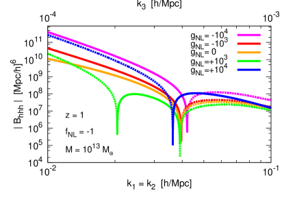
(a)

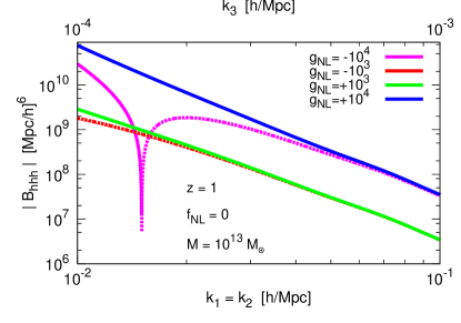
(b)

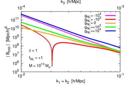
(c)

Figure 1:

Top: The absolute value of the halo bispectrum $B_{hhh}$ in the squeezed configuration $k_{1}=k_{2}=100k_{3}$, for halo mass $M=10^{13}M_{\odot}$, redshift $z=1$, $f_{\rm NL}=-1$. Different lines correspond to the values $g_{\rm NL}=0,\pm 10^{3},\pm 10^{4}$. We use solid lines to describe positive values and dotted lines for neagative values; the presence of a cusp indicates a change of sign. The pattern of zeros in the plotted range of wavenumbers can be used to distinguish $f_{\rm NL}$ from $g_{\rm NL}$: see the text for further details.
Bottom left: Same as the top panel, but for $f_{\rm NL}=0$. For $g_{\rm NL}=-10^{4}$ a zero is present.
Bottom right: Same as top panel, but for $f_{\rm NL}=1$. Notice that a single zero appears, for $g_{\rm NL}=-10^{3}$.

An inspection of these plots suggests an important qualitative feature of these results. If the parameters are contained within appropriate intervals, the halo bispectrum as a function of $k$ changes sign more times if $g_{\rm NL}$ has opposite sign with respect to $f_{\rm NL}$. For example, in Fig. 1, Case 1 corresponding to $f_{\rm NL}=-1$, we see that the green curve, corresponding to the logarithm of the bispectrum for $g_{\rm NL}=10^{3}$, changes sign twice instead of once as the other curves. Moreover, the positions of the zero at smaller scales, that exists for all the curves, depends on the value of $g_{\rm NL}$. In Fig. 1, Case 2 with $f_{\rm NL}=0$, the bispectra for different values of $g_{\rm NL}$ never change sign in the interval of scales we consider. Finally, in Fig. 1, Case 3 with $f_{\rm NL}=+1$, the red curve with $g_{\rm NL}\,=\,-10^{3}$ changes sign while all the other curves do not.

The qualitative features in the bispectra profiles as a function of scale become even more pronounced when considering higher redshifts or higher mass objects. To show this behaviour, we present plots displaying the halo bispectrum for two additional cases. The first set, displayed in Fig. 2, is for $M=10^{13}M_{\odot}$, $z=2$, $\epsilon=100$, while the second one is for $M=10^{14}M_{\odot}$, $z=1$, $\epsilon=100$ and is displayed in Fig. 3. Each plot uses the same conventions as Fig. 1. The qualitative considerations we made above are still valid. In particular, we see, at higher mass or redshift than our fiducial choice ($M=10^{13}M_{\odot}$, $z=1$, $\epsilon=100$), an increase in the absolute value of the halo bispectrum. Interestingly, the various contributions to the bispectrum weighted by different powers of $k$ make the magenta curve for $g_{\rm NL}=-10^{4}$ in the plots with $f_{\rm NL}=+1$ change sign, in both cases presented here. This new feature is due to the dependence of the bias parameters $b_{1}$, $b_{2}$ on mass and redshift.

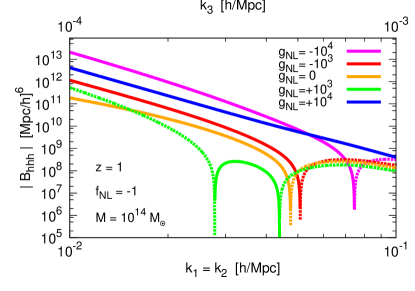
(a)

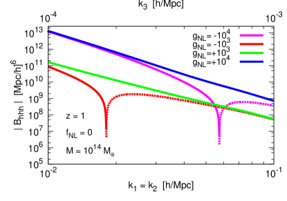
(b)

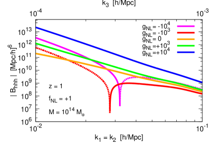
(c)

Figure 2:

Same as Fig. 1, but for $M=10^{14}M_{\odot}$. The amplitude of the bispectra have increased considerably over the case with $M=10^{13}M_{\odot}$ (shown in Fig. 1), the positions of the zeros have changed for $f_{NL}=-1$ (top panel, and the number of zeros has increased for $f_{NL}=0,+1$ (bottom right panel).

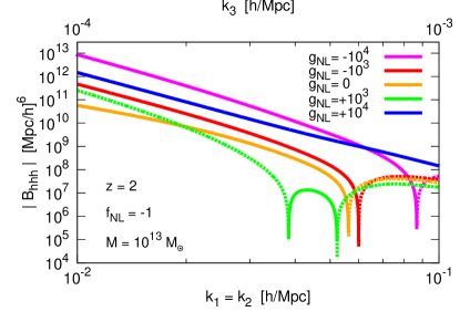
(a)

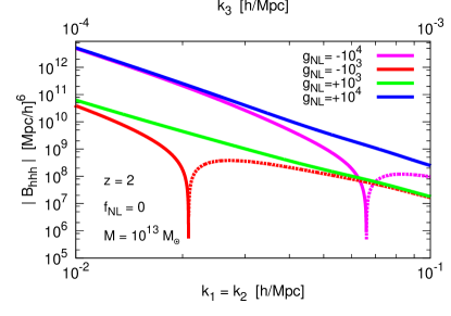
(b)

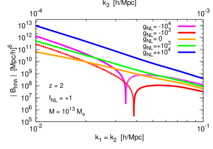
(c)

Figure 3:

Same as Fig. 1, but for $z=2$. The amplitude of the bispectra have increased significantly over the case of $z=1$ (shown in Fig. 1) and the positions of the zeros differ from those observed both in Fig. 1 and Fig. 2.

Hence, the previous plots show that the presence or absence of $g_{\rm NL}$ affects the bispectra profiles: in particular it governs how many times the halo bispectrum changes sign as a function of the scale. We already discussed this qualitative behavior in Section III.2.1, when analytically studying the roots of the bispectrum in the large scale limit. The numerical results of this section confirm those analytical findings, indicating that the qualitative profile of the halo bispectrum for isosceles triangles as a function of the scale can provide an interesting signature of the presence of $g_{\rm NL}$. Hence, we learn that the fact that the bispectrum changes sign in multiple locations as a function of the scale is a distinctive signal of the presence of $g_{\rm NL}$. Optimistically, this can be used to constraint values of $g_{\rm NL}$ smaller than the ones that can be tested by CMB. These features might be observed in cases in which large values of $b_{g}$ are realized, since in this case the bispectrum generated by primordial nG is more significant. Thus, the bispectrum is greater for larger halo masses $M$ and, at constant $M$, greater at higher redshift. For example, in Fig. 4 we provide an example of halos at redshift $z=2$, for $f_{\rm NL}=-1$. In this case, we see that the green curve corresponding to the halo bispectrum changes sign twice for $g_{\rm NL}=400$. An observation of this phenomenon can then probe quite small values for $g_{\rm NL}$. We can also compare the results of Fig. 4 with the analytical formulae for the zeros of the bispectrum, eqs (57) and (58). For the halo mass, redshift and $\epsilon$ parameter we are considering, we find $b_{g}\,\simeq\,4.3$, $\beta_{2}\,\simeq\,9.5$, $\beta_{3}\,\simeq\,1.1\,\times\,10^{-3}$. Computing the positions of the zeros of the bispectrum for the case $g_{\rm NL}=400$ with the analytical formulae of eqs (57) and (58), one finds the zeros at $k_{root}^{(1)}\simeq 1.2\cdot 10^{-2}$ and $k_{root}^{(2)}\simeq 4.9\cdot 10^{-2}$ h/Mpc, in agreement with the numerical results within one order of magnitude. This implies that our analytical findings, although obtained in the approximation in which we neglect the scale dependence of the transfer function, provide reasonably accurate predictions for the positions of the zeroes.

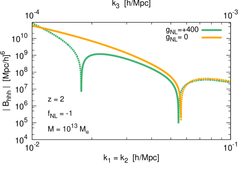
(a)

Figure 4:

The plot shows the absolute value of the halo bispectrum $B_{hhh}$ in the squeezed configuration $k_{1}=k_{2}=100k_{3}$, for halo mass $M=10^{13}M_{\odot}$ and redshift $z=2$. $f_{\rm NL}$ is kept constant and equal to $-1$, while different lines correspond to the values $g_{\rm NL}=0,400$. We use solid lines to describe positive values and dotted lines for negative values; the presence of a cusp indicate a change of sign. $f_{\rm NL}=-1$ produces a specific pattern of zeros in the line with $g_{\rm NL}=400$. If this feature can be observed in the halo bispectrum, it will improve the constrain on $g_{\rm NL}$ to few hundreds.

We now present a plot that represents the second theoretical observation we made in the previous sections: if it is possible to probe and observe bispectra correlating halo and matter densities (for example using gravitational lensing) then by analyzing combinations such as $C_{fnl}$ of eq. (60) we can have clean measurements of $f_{\rm NL}$ only, with a negligible contamination of $g_{\rm NL}$. In Fig. 5 we represent this quantity for different values of $f_{\rm NL}$, halo masses and redshifts; the lines are practically insensitive on $g_{\rm NL}$, and depend only on $f_{\rm NL}$ and on the halo mass. This feature, as we discussed around eq. (60), is valid at all scales (although at smaller scales one should take into more proper account the non-linear effects of gravity). This concretely shows that an observation of a non-vanishing value for the quantity $C_{fnl}$ would be a clean indication of a non-vanishing $f_{\rm NL}$. Combined with other measurements (for example associated with power spectra) this fact could then be used to obtain independent constraints on $g_{\rm NL}$.

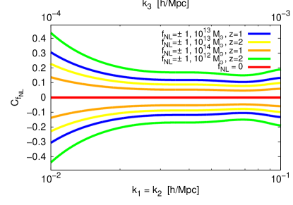
(a)

Figure 5:

The plot shows the quantity $C_{fnl}$ in the squeezed configuration $k_{1}=k_{2}=100k_{3}$, for different halo masses ($M=10^{12}M_{\odot},10^{13}M_{\odot},10^{14}M_{\odot}$) and redshifts ($z=1,2$). $C_{fnl}$ is positive for $f_{\rm NL}=+1$ and negative for $f_{\rm NL}=-1$. Remarkably, the lines are insensitive to the values of $g_{\rm NL}$.

We conclude that the scale dependence of bispectra of isosceles configurations in momentum space have qualitative features that might allow us to distinguish the effects of different nG parameters, in a way that is not possible by studying power spectra only.

While in the previous discussion we neglected the effects of non-linear gravity in the results for the bispectra, let us end this section with a preliminary analysis of its contributions. Focussing on squeezed configurations, the next plot shows a comparison between the amplitude of bispectra associated with primordial nG only (color lines) and bispectra due uniquely to the non-linear effects of gravity (black lines). We divide the bispectrum due to gravity in two contributions. The black dotted line corresponds to the amplitude of bispectra associated only with linear bias $b_{g\,0}$, and is controlled by the so-called $F_{2}$ function. This corresponds to the three point function for first order fluctuations. The black continuous line, instead, is the contribution associated with the quadratic coefficient $B_{2}$ of the local nonlinear biasing model of Fry:1992vr . We make the choice $B_{2}\,=\,2\,b_{g\,0}$ in order to be more conservative respect to Jeong:2009vd (See the review Bernardeau:2001qr for more details.)

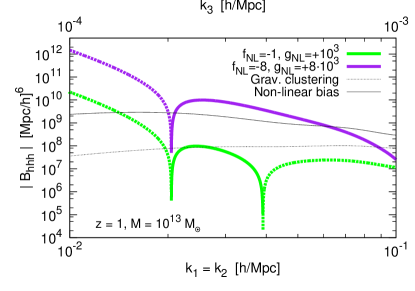
(a)

Figure 6:

The plot shows the amplitude of halo bispectra as a function of scale. The colored lines are bispectra associated with primordial nG only; the black lines are contributions to bispectra due to non-linear gravitational clustering. The black dotted line corresponds to the gravitational clustering contributions to $B_{hhh}$ depending on the linear bias $b_{g\,0}$ only. The continuous line is the gravity bispectrum associated with non-linear bias $b_{2}$ (we take $b_{2}\,=\,2b_{g\,0}$).

We notice that the amplitude of the bispectrum due to primordial nG tends to dominate at large scales (small $k$). However, if the primordial nG parameters are chosen to be small, the bispectrum induced by gravity is more important at smaller scales (see green line). For somewhat larger values of the nG parameters (with the magnitude of $g_{\rm NL}$ still below CMB constraints) the amplitude of the primordial bispectrum can dominate over the gravity contributions also at relatively small scales (see violet line). The primordial bispectrum represented in the violet line has non-trivial profile due to competing effects of primordial $f_{\rm NL}$ and $g_{\rm NL}$, in particular it has zeroes associated with the presence of $g_{\rm NL}$: if such features can be detected in the bispectrum profile, they can be used to help distinguishing among the effects of $f_{\rm NL}$ and $g_{\rm NL}$.

The plot above is only indicative, in the sense that one should study in more detail the combined effects of non-linear gravity and primordial nG in shaping the bispectra, and not only comparing their relative amplitude. On the other hand, it gives the idea that for interesting values of nG parameters the primordial contribution can lead to a rich profile for the bispectrum, controlled by the primordial nG parameters, with an amplitude larger or comparable to the one due to gravitational clustering only.

VII Discussion

Primordial nG characterizes the interactions of the fields sourcing the density fluctuations that seed the large-scale structure of our universe. In this work, using a generalized univariate approach that we compared with other methods in the literature, we analytically and numerically investigated how the statistics of LSS, in particular the study of bispectra of halos and matter, allow one to probe primordial nG. Our aim was to find ways to determine distinctive features of the local non-Gaussian parameters $f_{\rm NL}$ and $g_{\rm NL}$, controlling respectively skewness and kurtosis of the probability distribution function, and whose effects in the halo and matter power spectra are nearly degenerate. This investigation is important since although CMB constraints on $f_{\rm NL}$ have greatly improved with Planck, it is not clear whether CMB measurements only can set stringent constraints on $g_{\rm NL}$.

In the first part of this work, we showed analytically that the profiles of halo and matter bispectra have qualitative features that if measurable would clearly distinguish the effects of each non-Gaussian parameter. We exploited the scale dependence of the halo bias induced by primordial nG. We worked in a simplified situation in which only linear bias and linear effects of gravitational clustering are taken into account, to single out the effects of primordial nG in the statistics of LSS. We have shown that the profile of the halo bispectrum as a function of the scale, for isosceles configurations of triangles in momentum space, has properties that provide simple, qualitative information on each non-Gaussian parameter. For example, the number and the position of the zeros of this function depend on the size of $g_{\rm NL}$, and can be analytically computed with our formulae. If $g_{\rm NL}$ is present, and its sign is opposite with respect to the sign of $f_{\rm NL}$, the number of zeros of the bispectra increases as a function of the scale. Then, we determined a particular combination of halo and matter bispectra and power spectra, denoted $C_{fnl}$, that is proportional to $f_{\rm NL}$ only and is (nearly) independent on the value of $g_{\rm NL}$. A detection of this combination would be a clean probe of $f_{\rm NL}$ with no contaminations associated with $g_{\rm NL}$. We then generalized our findings to the case in which multiple sources contribute to form the primordial density fluctuations, and studied how stochastic halo bias is affected by the presence of $g_{\rm NL}$. We also provided new ways to study stochastic halo bias in terms of combinations of bispectra and power spectra.

In the second part of this work, we numerically confirmed and further developed our analytical results, focussing on a Press-Schechter approach to halo formation supplemented by appropriate non-Gaussian initial conditions. This analysis allowed us to apply our theoretical formulae for the bispectra focussing on scales and redshifts that might be probed by future surveys. We confirmed our theoretical considerations, showing plots representing how the qualitative profiles of halo bispectra in suitable configurations depend on non-Gaussian parameters, and might be used to set constraints on them. We ended our discussion with a preliminary analysis of the contributions of non-linear gravitational clustering, indicating that non-linear gravity tends to contaminate the bispectrum profiles, but that the qualitative features we investigated survive for sufficiently large primordial non-Gaussian parameters.

Our results can be extended in various directions. From the theoretical side, the non-linear effects associated with features of the mass function, bias and gravitational clustering (the non-linear transformation from Lagrangian to Eulerian coordinates), as well as loop effects, should be properly included in the context of perturbation theory, in order to understand whether and how primordial nG controls the qualitative features of bispectra also after taking these non-linearities into account. Having a good control of gravitational effects would also allow one to reliably study the bispectra for smaller values of the scale and for configurations that are less squeezed than the ones we considered here, and extend the validity of our results in these regimes. We plan to explore this interesting issue in a future publication. Another direction of investigation is a more systematic study of observational applications of our results, trying to quantify whether the methods we propose are sufficiently efficient to set constraints on $g_{\rm NL}$ that are more stringent than those available from the CMB. An important extension of our work is thus to forecast the signal-to-noise of galaxy bispectra as a function of scale, for future surveys such as EUCLID, and thereby test whether the features we predict are observable. Such study will exploit our theoretical inputs to develop optimised methods to distinguish the effects of $f_{\rm NL}$ and $g_{\rm NL}$ using galaxy bispectra and thus quantify their size and sign independently.

Acknowledgments

We thank Tommaso Giannantonio and Kazuya Koyama for useful discussions. GT is supported by an STFC Advanced Fellowship ST/H005498/1. DW is supported by STFC grant ST/K00090X/1. GT and DW thank the participants of the workshop “Constraining the early universe in the post Planck era”, funded by the Royal Society, for useful feedback on this work.

Appendix A Comparison with previous works

In this appendix, we compare our results with the ones obtained in two previous papers that studied galaxy bispectra.

We start discussing a comparison with the paper of Jeong and Komatsu Jeong:2009vd . Jeong and Komatsu were the first to investigate the halo bispectrum up to the nG parameter $g_{\rm NL}$ including the scale dependence of bias. It is important to point out the connection between their results and our findings. We address the issue in this Appendix.

First of all, let us briefly sketch the formalism used in Jeong:2009vd . They assume that the halo density contrast can be expressed as a local bias expansion of the matter overdensity in Eulerian coordinates, whose Fourier transform is

$$\delta_{h}(\vec{k})=B_{1}\delta_{M}(\vec{k})+\frac{B_{2}}{2}\left[\int\frac{d^{3}q}{(2\pi)^{3}}\delta_{M}(\vec{k}-\vec{q})\delta_{M}(\vec{q})-\sigma_{M}^{2}\delta^{(3)}(\vec{k})\right]+\dots,$$ (127)

where

$$\delta_{M}(\vec{k})=W_{M}(k)\left[\delta^{(1)}(\vec{k})+\delta^{(2)}(\vec{k})+\delta^{D}(\vec{k})+\dots\right]$$ (128)

and $\delta^{(1)}(\vec{k})=\alpha(k)\Phi(\vec{k})$ , while $\delta^{(n)}(\vec{k})$ is the $n$-th order quantity of the linear density contrast, given by perturbation theory Bernardeau:2001qr . The advantage of this approach is that non-linear evolution is automatically included when building the $3$-point function, even though calculations become harder.

On the other hand, the assumptions that led us to the halo density contrast of Eq.(27) are somewhat different. As we will show, the peak-background split method within a barrier crossing approach allows to re-obtain part of the results of Jeong:2009vd in a simple way (at least in the squeezed limit) and extend them up to higher powers of nG parameters. However, since we have not yet accounted for the non-linear effects of gravity, a comparison is possible only between primordial nG effects at this stage. Moreover, it is known (see for example Matsubara:2011ck ) that the local Lagrangian and Eulerian bias are not compatible in non-linear regimes.

By plugging Eqs.(28), (29), (30) into eq.(47) and collecting all the terms proportional to the same nG parameter, we find:

$$B_{hhh}^{f_{\rm NL}} = f_{\rm NL}\Delta_{0}^{2}b_{g}^{3}\frac{\alpha^{(1)}\alpha^{(2)}\alpha^{(3)}}{k_{1}^{3}k_{2}^{3}k_{3}^{3}}(k_{1}^{3}+k_{2}^{3}+k_{3}^{3})\simeq\,4f_{\rm NL}\Delta_{0}^{2}b_{g}^{3}\alpha^{3}_{0}\epsilon\,,$$ (129)

$$B_{hhh}^{f_{\rm NL}^{2}} = f_{\rm NL}^{2}\Delta_{0}^{2}b_{g}^{2}\beta_{2}\frac{\alpha^{(1)}\alpha^{(2)}\alpha^{(3)}}{k_{1}^{3}k_{2}^{3}k_{3}^{3}}\left[k^{3}_{1}\left(\frac{1}{\alpha^{(2)}}+\frac{1}{\alpha^{(3)}}\right)+\mbox{perm.}\right]\simeq\,4f_{\rm NL}^{2}\Delta_{0}^{2}b_{g}^{2}\beta_{2}\alpha_{0}^{2}\frac{\epsilon^{3}}{k^{2}}\,,$$ (130)

$$B_{hhh}^{g_{\rm NL}} = g_{\rm NL}\Delta_{0}^{2}b_{g}^{2}\beta_{2}\frac{\alpha^{(1)}\alpha^{(2)}\alpha^{(3)}}{k_{1}^{3}k_{2}^{3}k_{3}^{3}}\left(\frac{k_{1}^{3}}{\alpha^{(1)}}+\frac{k_{2}^{3}}{\alpha^{(2)}}+\frac{k_{3}^{3}}{\alpha^{(3)}}\right)\simeq\,6g_{\rm NL}\Delta_{0}^{2}b_{g}^{2}\beta_{2}\alpha_{0}^{2}\frac{\epsilon}{k^{2}},$$ (131)

where the approximated results are obtained by using $\alpha(k)\,=\,\alpha_{0}\,k^{2}$ and $T(k/\epsilon)\simeq T(k)$, in the squeezed configuration $k=k_{1}=k_{2}=\epsilon\,k_{3}$ with large $\epsilon$. The term $B_{hhh}^{f_{\rm NL}}$ is the same primordial nG contribution found in Jeong:2009vd ; Scoccimarro:2003wn ; Sefusatti:2007ih , while the approximated results for $B_{hhh}^{f_{\rm NL}^{2}}$ and $B_{hhh}^{g_{\rm NL}}$ match respectively those of eq.$(50)$ and eq.$(49)$ of Jeong:2009vd on large scales. However, a subtle difference between our results and those of Jeong:2009vd arise, due to the different initial assumptions. The matching is truly correct only if the equalities $B_{1}\equiv b_{g}$, $\beta_{2}\equiv 2B_{2}$ hold: it would be interesting to understand the physical meaning of this fact.

Some interesting consideration follow from the ratios of the previous quantities:

$$\frac{B_{hhh}^{f_{\rm NL}}}{B_{hhh}^{f_{\rm NL}^{2}}} = \frac{1}{f_{\rm NL}}\frac{b_{g}}{\beta_{2}}\frac{\alpha_{0}k^{2}}{\epsilon^{2}}\,,$$ (132)

$$\frac{B_{hhh}^{f_{\rm NL}}}{B_{hhh}^{g_{\rm NL}}} = \frac{2}{3}\frac{f_{\rm NL}}{g_{\rm NL}}\frac{b_{g}}{\beta_{2}}\alpha_{0}k^{2}\,,$$ (133)

$$\frac{B_{hhh}^{f_{\rm NL}^{2}}}{B_{hhh}^{g_{\rm NL}}} = \frac{2}{3}\frac{f_{\rm NL}^{2}}{g_{\rm NL}}\epsilon^{2}.$$ (134)

It is clear from the first ratio that the $f_{\rm NL}^{2}$ term can dominate over the $f_{\rm NL}$ one in the squeezed limit, as pointed out in Jeong:2009vd . Moreover, the bispectrum distinguishes between $B_{hhh}^{g_{\rm NL}}$ and $B_{hhh}^{f_{\rm NL}}$ (second ratio) but, surprisingly, the $g_{\rm NL}$ term shows the same scaling as the $f_{\rm NL}^{2}$ one.

At this point, all the primordial nG contributions found in Jeong:2009vd have been recovered but new terms come out from eq.(101). We collect them explicitly here:

$$B_{hhh}^{f_{\rm NL}^{3}} = \,f_{\rm NL}^{3}\Delta_{0}^{2}b_{g}\beta_{2}^{2}\left(\frac{\alpha^{(1)}}{k_{2}^{3}k_{3}^{3}}+\frac{\alpha^{(2)}}{k_{1}^{3}k_{3}^{3}}+\frac{\alpha^{(3)}}{k_{1}^{3}k_{2}^{3}}\right)\simeq\,4f_{\rm NL}^{3}\Delta_{0}^{2}b_{g}\beta_{2}^{2}\alpha_{0}\frac{\epsilon^{3}}{k^{4}}\,,$$ (135)

$$B_{hhh}^{f_{\rm NL}g_{\rm NL}} = f_{\rm NL}g_{\rm NL}\Delta_{0}^{2}b_{g}\frac{\alpha^{(1)}\alpha^{(2)}\alpha^{(3)}}{k_{1}^{3}k_{2}^{3}k_{3}^{3}}\left\{b_{g}\beta_{3}\left[k^{3}_{1}\left(\frac{1}{\alpha^{(2)}}+\frac{1}{\alpha^{(3)}}\right)+\mbox{perm.}\right]+\beta_{2}^{2}\left[\frac{k^{3}_{1}}{\alpha^{(1)}}\left(\frac{1}{\alpha^{(2)}}+\frac{1}{\alpha^{(3)}}\right)+\mbox{perm.}\right]\right\}\simeq$$ (136)

$$\simeq 2f_{\rm NL}g_{\rm NL}\Delta_{0}^{2}b_{g}\epsilon^{3}\left(2\frac{b_{g}\beta_{3}\alpha_{0}^{2}}{k^{2}}+3\frac{\beta_{2}^{2}\alpha_{0}}{k^{4}}\right)\,,$$

$$B_{hhh}^{g_{\rm NL}^{2}} = g_{\rm NL}^{2}\Delta_{0}^{2}b_{g}\beta_{2}\beta_{3}\left(\frac{\alpha^{(1)}+\alpha^{(2)}}{k_{1}^{3}k_{2}^{3}}+\frac{\alpha^{(1)}+\alpha^{(3)}}{k_{1}^{3}k_{3}^{3}}+\frac{\alpha^{(2)}+\alpha^{(3)}}{k_{2}^{3}k_{3}^{3}}\right)\simeq 6g_{\rm NL}^{2}\Delta_{0}^{2}b_{g}\beta_{2}\beta_{3}\alpha_{0}\frac{\epsilon^{3}}{k^{4}}\,,$$ (137)

$$B_{hhh}^{f_{\rm NL}^{2}g_{\rm NL}} = \,f_{\rm NL}^{2}g_{\rm NL}\Delta_{0}^{2}\left[\beta_{2}^{3}\left(\frac{1}{k_{1}^{3}k_{2}^{3}}+\frac{1}{k_{1}^{3}k_{3}^{3}}+\frac{1}{k_{2}^{3}k_{3}^{3}}\right)+2\beta_{2}\beta_{3}\left(\frac{\alpha^{(3)}}{k_{1}^{3}k_{2}^{3}}+\frac{\alpha^{(2)}}{k_{1}^{3}k_{3}^{3}}+\frac{\alpha^{(1)}}{k_{2}^{3}k_{3}^{3}}\right)\right]\simeq$$ (138)

$$\simeq \,2f_{\rm NL}^{2}g_{\rm NL}\Delta_{0}^{2}\epsilon^{3}\left(4\frac{b_{g}\beta_{2}\beta_{3}\alpha_{0}}{k^{4}}+3\frac{\beta_{2}^{3}}{k^{6}}\right)\,,$$

$$B_{hhh}^{f_{\rm NL}g_{\rm NL}^{2}} = \,f_{\rm NL}g_{\rm NL}^{2}\Delta_{0}^{2}\left[2\beta_{2}^{2}\beta_{3}\left(\frac{1}{k_{1}^{3}k_{2}^{3}}+\frac{1}{k_{1}^{3}k_{3}^{3}}+\frac{1}{k_{2}^{3}k_{3}^{3}}\right)+b_{g}\beta_{3}^{2}\left(\frac{\alpha^{(3)}}{k_{1}^{3}k_{2}^{3}}+\frac{\alpha^{(2)}}{k_{1}^{3}k_{3}^{3}}+\frac{\alpha^{(1)}}{k_{2}^{3}k_{3}^{3}}\right)\right]$$ (139)

$$\simeq \,4f_{\rm NL}g_{\rm NL}^{2}\Delta_{0}^{2}\epsilon^{3}\left(\frac{b_{g}\beta_{3}^{2}\alpha_{0}}{k^{4}}+3\frac{\beta_{2}^{2}\beta_{3}}{k^{6}}\right)\,,$$

$$B_{hhh}^{g_{\rm NL}^{3}} = \,g_{\rm NL}^{3}\Delta_{0}^{2}\beta_{2}\beta_{3}^{2}\left(\frac{1}{k_{1}^{3}k_{2}^{3}}+\frac{1}{k_{1}^{3}k_{3}^{3}}+\frac{1}{k_{2}^{3}k_{3}^{3}}\right)\simeq\,6g_{\rm NL}^{3}\Delta_{0}^{2}\beta_{2}\beta_{3}^{2}\frac{\epsilon^{3}}{k^{6}}\,.$$ (140)

These additional terms appear naturally within our framework and suggest that higher powers of nG parameters can in principle dominate over the lower ones, extending what Jeong and Komatsu found for the ratio $B_{hhh}^{f_{\rm NL}^{2}}/B_{hhh}^{f_{\rm NL}}$. All the contributions above are important for the specific features of the halo bispectrum discussed in section VI.

Let us now compare our approach with the one by Baldauf et al in Baldauf:2010vn . The easiest way to proceed is to reconsider our equation (27): by substituting our results for the bias coefficients $b_{i}$ (see eqs (28)-(30)), and using the relation $\delta_{L}\,=\,\alpha\,\Phi_{L}$, we can schematically write our expression for $\delta_{h}$ as an expansion

$$\delta_{h}\,=\,b_{g}\,\delta_{L}+\beta_{2}\,f_{\rm NL}\,\varphi_{L}+\beta_{3}\,g_{\rm NL}\,\varphi_{L}+b_{g}\,f_{\rm NL}\,\delta_{L}\varphi_{L}+\frac{3}{2}\,\beta_{2}\,g_{\rm NL}\,\varphi_{L}^{2}+b_{g}\,g_{\rm NL}\,\delta_{L}\,\varphi_{L}^{2}\,,$$ (141)

where to render the expression more compact, we understand the subtraction of the averages contained in (27). This ‘bivariate’ way of re-express our formula for the halo bias makes clear the connection with the bivariate approach of Giannantonio:2009ak ; Baldauf:2010vn , in which the Lagrangian halo bias is expanded in powers of $\delta_{L}$ and $\varphi_{L}$:

$$\delta_{h}\,=\,b_{10}\,\delta_{L}+b_{01}\,\varphi_{L}+\frac{b_{20}}{2}\,\delta_{L}^{2}+\frac{b_{02}}{2}\,\varphi_{L}^{2}+b_{11}\,\varphi_{L}\,\delta_{L}+\,\dots\,,$$ (142)

where the bias coefficient $b_{ij}$ is defined as

$$b_{ij}=\frac{1}{\bar{n}_{h}}\left(\frac{\partial^{i+j}n_{h}}{\partial^{i}\delta_{L}\partial^{j}\varphi_{L}}\right)\biggr{|}_{\delta_{L}=0,\varphi_{L}=0}\quad.$$ (143)

The values we find for the $b_{ij}$ coefficients are obtained by comparing eqs. (141) with (142):

$$b_{10} = b_{g}$$ (144)

$$b_{01} = \beta_{2}f_{\rm NL}+\beta_{3}g_{\rm NL}$$ (145)

$$b_{11} = b_{g}f_{\rm NL}$$ (146)

$$b_{02} = 3\beta_{2}\,g_{\rm NL}$$ (147)

$$b_{20} = 0$$ (148)

They differ from the ones of Giannantonio:2009ak ; Baldauf:2010vn for two reasons. The first reason is that, as explained in the main text, in our approach we decided to perform a Taylor expansion at linear order in $\delta$ and on all its correlation functions in Langrangian space. In this way we consider only non-linear effects induced by primordial nG, and we exclude non-linearities associated with higher derivatives of the mass function. This approximation is also justified by the fact that higher derivatives of the mass function along non-Gaussian parameters are under less reliable theoretical control. The second reason is that we include also the effects of (first) derivatives of the mass function along $f_{\rm NL}$ (that provide contributions proportional to $\beta_{3}$) that are instead neglected in a bivariate approach. Hence, for example, the coefficient $b_{01}$ in eq (145), using our definition of $\beta_{2}$, $\beta_{3}$ reads

$$b_{01} = \frac{2}{\bar{n}_{h}}\,\frac{\partial\,n_{h}}{\partial\,\ln{\sigma_{M}}}\,f_{\rm NL}+\frac{3}{\bar{n}_{h}}\,\frac{\partial\,n_{h}}{\partial\,f_{\rm NL}}\,g_{\rm NL}$$ (149)

While the first term can be associated with the analogous result reported in Giannantonio:2009ak ; Baldauf:2010vn , the second term is absent in their case. Indeed, the bivariate approach produces the $g_{\rm NL}/k^{2}$ dependence in the bias of the halo-halo and halo-matter power spectra as a contribution from the trispectrum Giannantonio:2009ak . On the other hand, our expression for $b_{20}$ is vanishing because we decided not to consider the second derivatives of $n_{h}$ along $\delta_{L}$. For the same reason of not considering such second derivatives, various contributions in the remaining coefficients $b_{ij}$ proportional to $f_{\rm NL}^{2}$, found in Giannantonio:2009ak ; Baldauf:2010vn are absent in our formulae.

Appendix B Inequalities among non-Gaussian parameters

In this appendix we collect some technical results on inequalities among primordial non-Gaussian parameters, that we use in Section V. The most famous of these inequalities is dubbed Suyama-Yamaguchi inequality, and relates the collapsed limit of the 4-pt function with the square of the squeezed limit of a 3-pt function of a given fluctuation $\delta$ in Fourier space Suyama:2007bg

$$\lim_{q\to 0}\,\langle\delta_{k_{1}}\delta_{-k_{1}-q}\delta_{k_{2}}\delta_{-k_{2}+q}\rangle^{\prime}\,\,\geq\,\,\lim_{q\to 0}\frac{\langle\delta_{k_{1}}\delta_{-k_{1}-q}\delta_{q}\rangle^{\prime 2}}{\langle\delta_{k_{1}}\delta_{q}\rangle}$$ (150)

Using the definitions for $\tau_{\rm NL}$ and $f_{\rm NL}$ and specializing to the case of primordial curvature fluctuations, this inequality corresponds to the Suyama-Yamaguchi inequality. It is convenient to simplify the notation, expressing the squeezed limit of the 3-pt function in (150) in a synthetic way as $\langle\delta[\delta^{2}]\rangle$, meaning that the momentum $q$ connecting $\delta$ and $[\delta^{2}]$ is sent to zero: this notation emphasizes that the long mode $\delta_{q}$ with $q\to 0$ modulates the 2-pt function $[\delta^{2}]$. Analogously, the collapsed limit of the 4-pt function can be expressed as $\langle[\delta^{2}][\delta^{2}]\rangle$. With the help of this notation, inequality (150) succinctly reads

$$\langle[\delta^{2}][\delta^{2}]\rangle\,\geq\,\frac{\langle\delta[\delta^{2}]\rangle^{2}}{\langle\delta\delta\rangle}$$ (151)

In Assassi:2012zq a simple proof of this inequality has been provided, by inserting a complete set of normalized momentum eigenstates $|n_{\vec{k}}\rangle\,\equiv\,|\delta_{k}\rangle/\langle\delta\delta\rangle^{\frac{1}{2}}$ into the quantity $\langle[\delta^{2}][\delta^{2}]\rangle$ of the left hand side of (151). The zero-momentum, long wavelength eigenstate provides the square of the squeezed 3pt function in the right hand side, to which one has to add the additional (positive definite) contributions that lead to the inequality above. In the collapsed limit and single source case, the additional contributions vanish and one saturates the inequality.

Although less explored in the literature, it is also possible to build further inequalities involving collapsed and squeezed limits of higher point functions (see for example Suyama:2011qi ; Byrnes:2011ri ): the virtue of the method of Assassi:2012zq is that the proofs of such inequalities can be straightforwardly generalized to those cases. As specific examples, we can write the following inequalities satisfied by five and six point functions, in appropriate collapsed limits

$$\langle[\delta^{3}][\delta^{2}]\rangle \geq \frac{\langle[\delta^{3}]\delta\rangle\langle[\delta^{2}]\delta\rangle}{\langle\delta\delta\rangle}$$ (152)

$$\langle[\delta^{3}][\delta^{3}]\rangle \geq \frac{\langle[\delta^{3}]\delta\rangle^{2}}{\langle\delta\delta\rangle}$$ (153)

Using the methods of Assassi:2012zq , it is relatively straightforward to prove that the inequalities saturate to equalities in the single source case. These inequalities have been used in Section V.1 for physically interpreting the notion of stochastic halo bias applied to power spectra of halos and matter. When considering stochastic halo bias for the bispectra, Section V.2 other inequalities are needed, that involve subtler collapsed limits among higher order point functions. We collect them here

$${\langle[\delta^{2}]\,[\delta^{2}]\,[\delta^{2}]\rangle} \geq \frac{{\langle\delta\,[\delta^{2}]\,[\delta^{2}]\rangle}{\langle\delta\,[\delta^{2}]\rangle}}{\langle\delta\,\delta\rangle}$$ (154)

$$\langle\delta\,[\delta^{2}]\,[\delta^{2}]\rangle \geq \frac{\langle\delta\,\delta\,[\delta^{2}]\rangle\langle\delta\,[\delta^{2}]\rangle}{\langle\delta\,\delta\rangle}$$ (155)

$$\langle\delta\,\delta\,[\delta^{2}]\rangle \geq \frac{\langle\delta\,\delta\,\delta\rangle\langle\delta\,[\delta^{2}]\rangle}{\langle\delta\,\delta\rangle}$$ (156)

They can be analyzed and proved again with the methods of Assassi:2012zq .

References

- (1) N. Bartolo, E. Komatsu, S. Matarrese and A. Riotto, “Non-Gaussianity from inflation: Theory and observations,” Phys. Rept. 402 (2004) 103 [astro-ph/0406398].
- (2) L. Verde and S. Matarrese, “Detectability of the effect of Inflationary non-Gaussianity on halo bias,” Astrophys. J. 706, L91 (2009) [arXiv:0909.3224 [astro-ph.CO]].
- (3) N. Bartolo, S. Matarrese, O. Pantano and A. Riotto, “Second-order matter perturbations in a LambdaCDM cosmology and non-Gaussianity,” Class. Quant. Grav. 27, 124009 (2010) [arXiv:1002.3759 [astro-ph.CO]].
- (4) M. Bruni, J. C. Hidalgo, N. Meures and D. Wands, “Non-Gaussian initial conditions in CDM: Newtonian, relativistic and primordial contributions,” arXiv:1307.1478 [astro-ph.CO].
- (5) P. A. R. Ade et al. [Planck Collaboration], “Planck 2013 results. I. Overview of products and scientific results,” arXiv:1303.5062 [astro-ph.CO].
- (6) T. Sekiguchi and N. Sugiyama, “Optimal constraint on from CMB,” arXiv:1303.4626 [astro-ph.CO].
- (7) J. Smidt, A. Amblard, C. T. Byrnes, A. Cooray, A. Heavens and D. Munshi, “CMB Constraints on Primordial non-Gaussianity from the Bispectrum () and Trispectrum ( and ) and a New Consistency Test of Single-Field Inflation,” Phys. Rev. D 81 (2010) 123007 [arXiv:1004.1409 [astro-ph.CO]].
- (8) S. Nurmi, C. T. Byrnes and G. Tasinato, “A non-Gaussian landscape,” JCAP 1306 (2013) 004 [arXiv:1301.3128 [astro-ph.CO]];
- (9) C. T. Byrnes and G. Tasinato, “Non-Gaussianity beyond slow roll in multi-field inflation,” JCAP 0908 (2009) 016 [arXiv:0906.0767 [astro-ph.CO]]; J. Emery, G. Tasinato and D. Wands, “Local non-Gaussianity from rapidly varying sound speeds,” JCAP 1208 (2012) 005 [arXiv:1203.6625 [hep-th]].
- (10) T. Suyama, T. Takahashi, M. Yamaguchi and S. Yokoyama, “Implications of Planck results for models with local type non-Gaussianity,” JCAP 1306 (2013) 012 [arXiv:1303.5374 [astro-ph.CO]].
- (11) N. Dalal, O. Dore, D. Huterer and A. Shirokov, “The imprints of primordial non-gaussianities on large-scale structure: scale dependent bias and abundance of virialized objects,” Phys. Rev. D 77 (2008) 123514 [arXiv:0710.4560 [astro-ph]].
- (12) A. Slosar, C. Hirata, U. Seljak, S. Ho and N. Padmanabhan, “Constraints on local primordial non-Gaussianity from large scale structure,” JCAP 0808 (2008) 031 [arXiv:0805.3580 [astro-ph]];
- (13) S. Matarrese and L. Verde, “The effect of primordial non-Gaussianity on halo bias,” Astrophys. J. 677 (2008) L77 [arXiv:0801.4826 [astro-ph]].
- (14) N. Afshordi and A. J. Tolley, “Primordial non-gaussianity, statistics of collapsed objects, and the Integrated Sachs-Wolfe effect,” Phys. Rev. D 78 (2008) 123507 [arXiv:0806.1046 [astro-ph]].
- (15) J. -O. Gong and S. Yokoyama, “Scale dependent bias from primordial non-Gaussianity with trispectrum,” arXiv:1106.4404 [astro-ph.CO].
- (16) V. Desjacques, U. Seljak and I. Iliev, “Scale-dependent bias induced by local non-Gaussianity: A comparison to N-body simulations,” Mon. Not. Roy. Astron. Soc. 396 (2009) 85 [arXiv:0811.2748 [astro-ph]].
- (17) V. Desjacques, D. Jeong and F. Schmidt, “Accurate Predictions for the Scale-Dependent Galaxy Bias from Primordial Non-Gaussianity,” Phys. Rev. D 84 (2011) 061301 [arXiv:1105.3476 [astro-ph.CO]].
- (18) V. Desjacques, D. Jeong and F. Schmidt, “Non-Gaussian Halo Bias Re-examined: Mass-dependent Amplitude from the Peak-Background Split and Thresholding,” Phys. Rev. D 84 (2011) 063512 [arXiv:1105.3628 [astro-ph.CO]].
- (19) V. Desjacques and U. Seljak, “Primordial non-Gaussianity from the large scale structure,” Class. Quant. Grav. 27 (2010) 124011 [arXiv:1003.5020 [astro-ph.CO]].
- (20) L. Verde, “Non-Gaussianity from Large-Scale Structure Surveys,” Adv. Astron. 2010 (2010) 768675 [arXiv:1001.5217 [astro-ph.CO]].
- (21) N. Roth and C. Porciani, “Can we really measure fnl from the galaxy power spectrum?,” arXiv:1205.3165 [astro-ph.CO].
- (22) V. Desjacques and U. Seljak, “Signature of primordial non-Gaussianity of -type in the mass function and bias of dark matter haloes,” Phys. Rev. D 81 (2010) 023006 [arXiv:0907.2257 [astro-ph.CO]].
- (23) T. Giannantonio, A. J. Ross, W. J. Percival, R. Crittenden, D. Bacher, M. Kilbinger, R. Nichol and J. Weller, “Improved Primordial Non-Gaussianity Constraints from Measurements of Galaxy Clustering and the Integrated Sachs-Wolfe Effect,” arXiv:1303.1349 [astro-ph.CO].
- (24) M. LoVerde, A. Miller, S. Shandera and L. Verde, “Effects of Scale-Dependent Non-Gaussianity on Cosmological Structures,” JCAP 0804 (2008) 014 [arXiv:0711.4126 [astro-ph]].
- (25) C. T. Byrnes, M. Gerstenlauer, S. Nurmi, G. Tasinato and D. Wands, “Scale-dependent non-Gaussianity probes inflationary physics,” JCAP 1010 (2010) 004 [arXiv:1007.4277 [astro-ph.CO]];
- (26) D. Jeong and E. Komatsu, “Primordial non-Gaussianity, scale-dependent bias, and the bispectrum of galaxies,” Astrophys. J. 703 (2009) 1230 [arXiv:0904.0497 [astro-ph.CO]].
- (27) E. Sefusatti, “1-loop Perturbative Corrections to the Matter and Galaxy Bispectrum with non-Gaussian Initial Conditions,” Phys. Rev. D 80 (2009) 123002 [arXiv:0905.0717 [astro-ph.CO]].
- (28) T. Nishimichi, A. Taruya, K. Koyama and C. Sabiu, “Scale Dependence of Halo Bispectrum from Non-Gaussian Initial Conditions in Cosmological N-body Simulations,” JCAP 1007 (2010) 002 [arXiv:0911.4768 [astro-ph.CO]].
- (29) E. Sefusatti, M. Crocce and V. Desjacques, “The Halo Bispectrum in N-body Simulations with non-Gaussian Initial Conditions,” arXiv:1111.6966 [astro-ph.CO].
- (30) D. Baumann, S. Ferraro, D. Green and K. M. Smith, “Stochastic Bias from Non-Gaussian Initial Conditions,” arXiv:1209.2173 [astro-ph.CO].
- (31) R. Scoccimarro, L. Hui, M. Manera and K. C. Chan, “Large-scale Bias and Efficient Generation of Initial Conditions for Non-Local Primordial Non-Gaussianity,” Phys. Rev. D 85 (2012) 083002 [arXiv:1108.5512 [astro-ph.CO]].
- (32) T. Giannantonio and C. Porciani, “Structure formation from non-Gaussian initial conditions: multivariate biasing, statistics, and comparison with N-body simulations,” Phys. Rev. D 81 (2010) 063530 [arXiv:0911.0017 [astro-ph.CO]].
- (33) C. T. Byrnes, S. Nurmi, G. Tasinato and D. Wands, “Inhomogeneous non-Gaussianity,” JCAP 1203 (2012) 012 [arXiv:1111.2721 [astro-ph.CO]].
- (34) D. Tseliakhovich, C. Hirata and A. Slosar, “Non-Gaussianity and large-scale structure in a two-field inflationary model,” Phys. Rev. D 82 (2010) 043531 [arXiv:1004.3302 [astro-ph.CO]].
- (35) F. Bernardeau, S. Colombi, E. Gaztanaga and R. Scoccimarro, “Large scale structure of the universe and cosmological perturbation theory,” Phys. Rept. 367 (2002) 1 [astro-ph/0112551].
- (36) S. D. M. White and M. J. Rees, “Core condensation in heavy halos: A Two stage theory for galaxy formation and clusters,” Mon. Not. Roy. Astron. Soc. 183 (1978) 341.
- (37) W. H. Press and P. Schechter, “Formation of galaxies and clusters of galaxies by selfsimilar gravitational condensation,” Astrophys. J. 187 (1974) 425.
- (38) S. Cole and N. Kaiser, “Biased clustering in the cold dark matter cosmogony,” Mon. Not. Roy. Astron. Soc. 237, 1127 (1989).
- (39) J. M. Bardeen, J. R. Bond, N. Kaiser and A. S. Szalay, “The Statistics of Peaks of Gaussian Random Fields,” Astrophys. J. 304 (1986) 15.
- (40) S. Ferraro, K. M. Smith, D. Green and D. Baumann, “On the Equivalence of Barrier Crossing, Peak-Background Split, and Local Biasing,” arXiv:1209.2175 [astro-ph.CO].
- (41) T. Baldauf, U. Seljak and L. Senatore, “Primordial non-Gaussianity in the Bispectrum of the Halo Density Field,” JCAP 1104 (2011) 006 [arXiv:1011.1513 [astro-ph.CO]].
- (42) S. Yokoyama, T. Matsubara and A. Taruya, “Halo/Galaxy Bispectrum with Primordial non-Gaussianity from integrated Perturbation Theory (iPT),” arXiv:1310.4925 [astro-ph.CO].
- (43) G. Tasinato, C. T. Byrnes, S. Nurmi and D. Wands, “Loop corrections and a new test of inflation,” Phys. Rev. D 87 (2013) 4, 043512 [arXiv:1207.1772 [hep-th]].
- (44) R. Laureijs et al. [EUCLID Collaboration], “Euclid Definition Study Report,” arXiv:1110.3193 [astro-ph.CO].
- (45) http://camb.info/
- (46) E. Komatsu et al. [WMAP Collaboration], “Five-Year Wilkinson Microwave Anisotropy Probe (WMAP) Observations: Cosmological Interpretation,” Astrophys. J. Suppl. 180 (2009) 330 [arXiv:0803.0547 [astro-ph]].
- (47) A. Pillepich, C. Porciani and O. Hahn, “Universal halo mass function and scale-dependent bias from N-body simulations with non-Gaussian initial conditions,” arXiv:0811.4176 [astro-ph].
- (48) M. Grossi, L. Verde, C. Carbone, K. Dolag, E. Branchini, F. Iannuzzi, S. Matarrese and L. Moscardini, “Large-scale non-Gaussian mass function and halo bias: tests on N-body simulations,” Mon. Not. Roy. Astron. Soc. 398 (2009) 321 [arXiv:0902.2013 [astro-ph.CO]].
- (49) S. Matarrese, L. Verde and R. Jimenez, “The Abundance of high-redshift objects as a probe of non-Gaussian initial conditions,” Astrophys. J. 541 (2000) 10 [astro-ph/0001366].
- (50) K. M. Smith, S. Ferraro and M. LoVerde, “Halo clustering and -type primordial non-Gaussianity,” JCAP 1203 (2012) 032 [arXiv:1106.0503 [astro-ph.CO]].
- (51) M. Maggiore and A. Riotto, “The Halo Mass Function from Excursion Set Theory with a Non-Gaussian Trispectrum,” Mon. Not. Roy. Astron. Soc. Lett. 405 (2010) 1244 [arXiv:0910.5125 [astro-ph.CO]].
- (52) M. LoVerde and K. M. Smith, “The Non-Gaussian Halo Mass Function with , and ,” JCAP 1108 (2011) 003 [arXiv:1102.1439 [astro-ph.CO]].
- (53) H. J. Mo and S. D. M. White, “An Analytic model for the spatial clustering of dark matter halos,” Mon. Not. Roy. Astron. Soc. 282 (1996) 347 [astro-ph/9512127].
- (54) A. J. Ross, W. J. Percival, A. Carnero, G. -b. Zhao, M. Manera, A. Raccanelli, E. Aubourg and D. Bizyaev et al., “The Clustering of Galaxies in SDSS-III DR9 Baryon Oscillation Spectroscopic Survey: Constraints on Primordial Non-Gaussianity,” arXiv:1208.1491 [astro-ph.CO].
- (55) L. Anderson, E. Aubourg, S. Bailey, D. Bizyaev, M. Blanton, A. S. Bolton, J. Brinkmann and J. R. Brownstein et al., “The clustering of galaxies in the SDSS-III Baryon Oscillation Spectroscopic Survey: Baryon Acoustic Oscillations in the Data Release 9 Spectroscopic Galaxy Sample,” Mon. Not. Roy. Astron. Soc. 427 (2013) 4, 3435 [arXiv:1203.6594 [astro-ph.CO]].
- (56) J. N. Fry and E. Gaztanaga, “Biasing and hierarchical statistics in large scale structure,” Astrophys. J. 413 (1993) 447 [astro-ph/9302009].
- (57) T. Matsubara, “Nonlinear Perturbation Theory Integrated with Nonlocal Bias, Redshift-space Distortions, and Primordial Non-Gaussianity,” Phys. Rev. D 83 (2011) 083518 [arXiv:1102.4619 [astro-ph.CO]].
- (58) R. Scoccimarro, E. Sefusatti and M. Zaldarriaga, “Probing primordial non-Gaussianity with large - scale structure,” Phys. Rev. D 69 (2004) 103513 [astro-ph/0312286].
- (59) E. Sefusatti and E. Komatsu, “The bispectrum of galaxies from high-redshift galaxy surveys: Primordial non-Gaussianity and non-linear galaxy bias,” Phys. Rev. D 76 (2007) 083004 [arXiv:0705.0343 [astro-ph]].
- (60) T. Suyama and M. Yamaguchi, “Non-Gaussianity in the modulated reheating scenario,” Phys. Rev. D 77 (2008) 023505 [arXiv:0709.2545 [astro-ph]].
- (61) T. Suyama and S. Yokoyama, “Extension of local-type inequality for the higher order correlation functions,” JCAP 1107 (2011) 033 [arXiv:1105.5851 [astro-ph.CO]].
- (62) V. Assassi, D. Baumann and D. Green, “On Soft Limits of Inflationary Correlation Functions,” JCAP 1211 (2012) 047 [arXiv:1204.4207 [hep-th]].