Conductance through disordered graphene nanoribbons: Standard and anomalous electron localization

Abstract

Conductance fluctuations produced by the presence of disorder in zigzag and armchair graphene nanoribbons are studied. We show that quantum transport in zigzag nanoribbons takes place via edge states which are exponentially localized, as in the standard Anderson localization problem, whereas for armchair nanoribbons the symmetry of the graphene sublattices produces anomalous localization, or delocalization. We show that these two different electron localizations lead to significant differences of the conductance statistics between zigzag and armchair nanoribbons. In particular, armchair nanoribbons show nonconventional large conductance fluctuations relative to those of Anderson-localized electrons. We calculate analytically the complete distribution of conductances for both types of ribbons. Without free fitting parameters, we verify our theoretical results by performing numerical simulations of disordered zigzag and armchair nanoribbons of experimentally achievable lengths and widths.

I introduction

Graphene remains one of the most studied materials since the experimental isolation of its two-dimensional honeycomb lattice from graphite.novoselov2004 The singular properties of graphene have attracted such an interest, from fundamental and application points of view, that nowadays an extensive literature exists on different physical phenomena occurring in this material. reviews The honeycomb arrangement of carbon atoms in graphene provides two relevant ingredients to electronic transport: a sublattice (chiral) symmetry and a linear dispersion relation. The latter, valid at low energies,wallace has attracted a lot of attention since it allows an analogy with relativistic massless particles described by the Dirac equation. However, the sublattice symmetry is perhaps a feature of more fundamental importance. The lattice structure of graphene is described by two identical interconnected sublattices, such that the sites of one sublattice are connected only to the sites of the other one, i.e., the lattice of graphene is bipartite resulting in a symmetric energy spectrum around the Fermi energy. The sublattice symmetry, also known as chiral symmetry, has deep consequences on different electronic properties, as has been shown in the past, soukoulis ; inui ; spiros1 although, there is a revived interest in the context of superconducting quasiparticles, topological insulators, and superconductors. altland ; schnyder ; xiao

Electronic properties of pristine graphene structures have been extensively studied. However, real graphene-based devices can be affected by the presence of disorder, as any other mesoscopic material. Different sources of disorder can be found in graphene. For instance, distortion of the lattice like ripples can appear by interactions with the substrate. gallagher ; melinda Experiments have been performed using suspended graphene structures to avoid effects of the substrate, meyer ; jarillo but even in this case graphene samples are not free of defects. Also, experimental evidence of short range disorder in graphene has been found in Refs. Tan, ; Jang, . Despite the fact that disorder is generally considered as an ingredient to be avoided, one might take advantage of it. For instance, electronic properties of graphene can be manipulated by doping a sample or by replacing carbon atoms. pi ; ruitao ; peres

Disorder plays a central role in the problem of quantum transport and therefore its effects have been widely studied. For instance, it is known that in one-dimensional (1D) systems, the presence of any small amount of disorder leads to exponential localization of electron wavefunctions (Anderson localization) with the distance $r$: $|\psi|\sim e^{-\gamma r}$. This exponential decay has been experimentally and theoretically studied in different disordered systems.phystoday The inverse of the localization length $\gamma$ is of fundamental importance for the description of statistical properties of transport within the scaling approach to localization.mello_book However, electron wavefunctions are not always exponentially (Anderson) localized; it has been shown that the wavefunction decays as $|\psi|\sim e^{-\gamma\sqrt{r}}$ at the band center of 1D systems with random hopping between neighboring lattice sites (off-diagonal disorder), i.e., electrons are less localized (delocalized) than in the standard Anderson problem.soukoulis ; spiros1

Several models have been used to describe different effects of disorder in graphene. The literature is very extensive and we turn the attention of the reader to Ref. mucciolo, for a review of the topic (see also Refs. areshkin, ; bardarson, ; kentaro, ; pablo, ; rossi, ; reviews, ; xiong, ; verges, ; evaldsson, ; libisch, ; wakabashi, ; ioannis_1, ; ioannis_2, ). For example, effective Hamiltonians (Dirac Hamiltonians) valid in the continuum low-energy limit and tight-binding models have been introduced to study statistical properties of conductance fluctuations, such as the density of transmission eigenvalues. areshkin ; bardarson ; kentaro ; pablo ; rossi ; reviews ; xiong ; verges ; evaldsson ; libisch ; wakabashi Most of the theoretical works, however, deal with effects produced by the standard Anderson-localization of electrons.

For finite-size graphene structures like nanoribbons, an additional element has to be considered in the study of quantum transport, namely, the sample terminations or edges. There are two different basic graphene edges: zigzag and armchair, which affect the electronic properties of nanoribbons. For example, the band structure is completely different for each termination (e.g., Fig. 1, bottom panels). Also, the existence of edge states in clean zigzag nanoribbons has been shown, nakada ; tao whereas in armchair nanoribbons those states are absent.

Detailed experimental investigations on the effects of graphene edges on quantum transport have been restricted by technological limitations on controlling the edge of graphene samples. Nowadays a precise manipulation of graphene terminations is still a challenge, but recent experiments have shown a high control of the nanoribbon edges.zhang In fact, transport experiments have been performed with an accurate control of the nanoribbon terminations. koch

Therefore, understanding the role of the edge morphology in nanoribbons as well as the effects of disorder in graphene-based devices is of interest from a fundamental point of view and relevant to future experimental investigations.

In this work, the effects of both disorder and edges on the conductance fluctuations of graphene nanoribbons are studied. We calculate the conductance distribution of disordered zigzag and armchair graphene nanoribbons. As we show below, electronic transport in zigzag nanoribbons takes place via standard exponentially localized states (Anderson localization), which allows us to study the conductance statistics within a conventional approach to localization. For armchair nanoribbons, however, electrons are delocalized and we require an extension of the standard localization approach. Thus, the conductance statistics is affected significatively by the nanoribbon edges.

II Numerical and theoretical models

Concerning the numerical results, we use a standard tight-binding Hamiltonian model to describe the armchair and zigzag graphene nanoribbons:

$$H=\sum_{\langle i,j\rangle}t_{i,j}(c_{i}^{\dagger}c_{j}+c_{j}^{\dagger}c_{i}),$$ (1)

where $i$ and $j$ are nearest neighbors and $c_{i}^{\dagger}$ ($c_{i}$) is the creation (annihilation) operator for spinless fermions. Disorder is introduced via random hopping elements $t_{i,j}$ connecting the two sublattices. This type of short-range disorder models the presence of distortions in graphene samples and preserves the symmetry of the graphene lattice. The $t_{i,j}$’s are sampled from the distribution $p(t)=1/wt$ with $\exp(-w/2)\leq t\leq\exp(w/2)$, where $w$ denotes the strength of the disorder (we fix $w=1$). Our numerical calculations are performed at the low energy $E=10^{-6}$ (in units of the hopping energy of the perfect leads). The length $L$ and width $W$ of the nanoribbons are reported in units of the lattice constant $a\simeq 2.46\textup{\AA}$. We have fixed $W=11a/\sqrt{3}$ for zigzag nanoribbons in our simulations, which corresponds to eight zigzag chains, while for armchair ribbons $W=5a$. The conductance $G$ (in units of the conductance quantum ${2e^{2}}/{h}$) is calculated by attaching perfect metallic graphene leads to the left and right side of the disordered ribbons (top panels in Fig. 1). We use a recursive Green’s function method li to calculate the conductance within the Landauer-Büttiker approach. The conductance statistics is obtained by collecting data over an ensemble of $2\times 10^{4}$ disorder realizations.

II.1 Disordered zigzag-nanoribbons

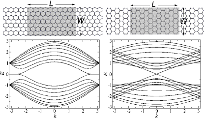
Figure 1: Top: Graphene nanoribbons with zigzag (left) and armchair (right) edges with disordered regions (shaded areas) of length $L$ and width $W$ attached to perfect leads. Bottom: Band structures calculated for the clean zigzag (left) and armchair (right) graphene nanoribbons of width $W=11a/\sqrt{3}$ and 5$a$, respectively.

From the band structure of pristine zigzag nanoribbons (bottom-left panel in Fig. 1), we see that only one channel is open at low energies ($E\lesssim 0.5$). On the other hand, it is known that edge states are present in perfect graphene samples with zigzag terminations.nakada When disorder is introduced, those states living at the border of the nanoribbon become exponentially localized. As an illustration of those edge localized states, in Fig. 2 (a) we show the modulus squared of the wavefunction for one realization of the disorder; we can see that the wavefunction is located on the border slightly penetrating the ribbon. In the Anderson localization problem, it is known that the conductance decays exponentially with the length $L$ and a signature of (Anderson) localization is the linear behavior of the average $\langle\ln G\rangle$ with $L$. We have obtained numerically such a linear relation, as can be seen in Fig. 2 (b).

The exponential localization of electrons for zigzag nanoribbons simplifies our analysis since, within a scaling theory of Anderson localization, the conductance distribution $P_{s}(G)$ is determined completely by the ratio $s\equiv L/l$, $l$ being the mean free path. mello_book ; melnikov ; dorokhov The exact expression for $P_{s}(G)$ is given in terms of quadratures. Here we provide a simpler expression:

$$P_{s}(G)=C\frac{\left[\mathrm{acosh}(1/\sqrt{G})\right]^{1/2}}{G^{3/2}(1-G)^{1/4}}e^{-(1/s)\mathrm{acosh}^{2}(1/\sqrt{G})},$$ (2)

where $C$ is a normalization constant. Equation (2) is an approximation to the exact solution of Mel’nikov equation (see the Appendix) and is useful for any practical value of $s$. The value of $s$ can be determined numerically through the relation $\langle-\ln G\rangle=L/l$. gopar-molina

We now compare some results from our expression Eq. (2) with numerical simulations of zigzag nanoribbons. In Fig. 2 (bottom) we show two numerical distributions (histograms) and the corresponding theoretical predictions (solid lines). The value of $s$ in Eq. (2) is extracted from our simulations [Fig. 2](b)]. We present two cases with very different average conductance: for Figs. 2(c) and (d), $\langle G\rangle$=0.46 and $\langle G\rangle=0.04$, respectively. Note that, while in Fig. 2(c) we show $P_{s}(G)$, in Fig. 2 (d) $P_{s}(\ln G)$ is plotted instead, as for small values of $\langle G\rangle$, the distribution $P_{s}(G)$ is very sharp. An excellent agreement between simulations and theory is seen in both panels (c) and (d) in Fig. 2.

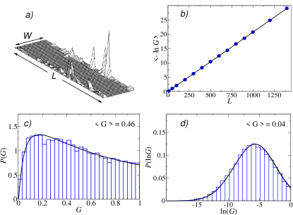
Figure 2: (Color online) (a) Modulus squared of the wavefunction of a zigzag nanoribbon sample. We can see that the wavefunction is concentrated along the border of the sample. According to the conductance fluctuations these edge states are exponentially (Anderson) localized. (b) The linear dependence of $\langle\ln G\rangle$ with $L$ for zigzag nanoribbons. The solid line is a linear fitting of the numerical data (dots). (c) Numerical (histogram) and theoretical (solid line) conductance distributions for $\langle G\rangle=0.46$ ($\langle-\ln G\rangle=1.03$). (d) Numerical (histogram) and theoretical (solid line) distributions of the logarithm of the conductance for the case $\langle G\rangle=0.04$ ($\langle-\ln G\rangle=6.21$). A good agreement is seen between numerical and theoretical distributions, in both panels (c) and (d).

II.2 Disordered armchair nanoribbons

We observe from the band structure in Fig. 1 (bottom-right) that only one channel contributes to the transport near the Fermi energy, as in the case of zigzag nanoribbons. Now, however, anomalous localization of electrons takes place. A signature of such delocalization is the nonlinear dependence of $\langle\ln G\rangle$ versus the length $L$. We illustrate this behavior in our armchair nanoribbons in Fig. 3(a), where a power-law dependence of $\langle\ln G\rangle$ with $L$ is shown. One might contrast this result with the linear dependence of $\langle\ln G\rangle$ with $L$ for zigzag nanoribbons [Fig. 2(b)].

Therefore anomalous localization is present in our armchair nanoribbons and we cannot study the electronic transport within the standard scaling approach of localization, Eq. (2).

A model to describe the statistical properties of transport when electron wavefunctions are anomalously localized has been proposed.fernando_gopar ; elias Within that model, the knowledge of just two quantities: the average $\langle\ln G\rangle$ and the exponent $\alpha$ in $\langle\ln G\rangle\propto L^{\alpha}$, is enough to calculate the complete distribution of conductances. Physically, $\alpha$ might be considered a measure of the strength of the electron localization: the localization becomes weaker as $\alpha$ decreases. With the above information, the conductance distribution $P_{\xi,\alpha}(G)$ can be obtained from

$$P_{\xi,\alpha}(G)=\int_{0}^{\infty}P_{s(\alpha,\xi,z)}(g)q_{\alpha,1}(z){\rm d}z,$$ (3)

where we have defined $\xi=\langle\ln G\rangle$. $P_{s(\alpha,\xi,z)}(G)$ is given by Eq. (2), $s$ being now a function defined as $s(\alpha,\xi,z)={\xi}/(2{z^{\alpha}I_{\alpha})}$, where $I_{\alpha}=1/2\int_{0}^{\infty}z^{-\alpha}q_{\alpha,1}dz$. The function $q_{\alpha,1}(z)$ is the probability density of the so-called $\alpha$-stable distributions ($\alpha<1$) supported in the positive semiaxis. No analytical expressions for $\alpha$-stable distributions exist, except for few special values of $\alpha$. We thus obtain $P_{\xi,\alpha}(G)$ by numerical integration.

As we pointed out, our theoretical model depends on $\alpha$ and $\langle\ln G\rangle$, which are extracted from the numerical simulations and then plugged into Eq. (3). From Fig. 3 we have extracted the value of $\alpha=0.69$. This value does not depend on the length, width, and degree of disorder, according to our numerical simulations; in this sense it is universal for graphene nanoribbons with off-diagonal disorder, at the band center.alpha1D Thus, in Figs. 3 (b) and 3(c) we compare the numerical (histograms) and theoretical (solid lines) distributions for two different conductance averages. In Fig. 3(b) we show $P(G)$ for a case with $\langle G\rangle=0.46$, while in Fig. 3(c), $\langle G\rangle=0.15$. Note that in the latter case we plot $P(\ln G)$ for convenience, as we previously explained. Thus, we see that our model describes the trend of the complete conductance distributions.

In order to remark the differences in the conductance fluctuations between zigzag and armchair disordered nanoribbons, we plot in Fig. 3(d) the distributions for both edge terminations with the same conductance average $\langle G\rangle=0.46$. We see that distributions are very different. We notice, for instance, that small conductances ($G\sim 0$) are suppressed for zigzag nanoribbons, in contrast to the case of armchair nanoribbons whose conductance distribution has a peak. In addition, large values of conductance ($G\sim 1$) are favored in armchair nanoribbons, in relation to the zigzag case.

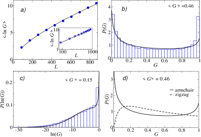
Figure 3: Color online (a) The nonlinear dependence of the average $\langle\ln G\rangle$ with $L$ for armchair nanoribbons. The solid line is obtained by fitting: $\langle\ln G\rangle\propto L^{\alpha}$ with $\alpha=0.69$. Inset: the power-law dependence is valid at all nanoribbon lengths, as shown by the single straight line obtained when plotting the data in log-log scale. (b) Numerical (histogram) and theoretical (solid line) distributions for armchair ribbons with $\langle G\rangle=0.46$ ($\langle-\ln G=1.37\rangle$). (c) Numerical (histogram) and theoretical (solid line) distributions $P(\ln G)$ for armchair ribbons with $\langle G\rangle=0.15$ ($\langle-\ln G\rangle=6.37$). In both panels (b) and (c) a good agreement is seen. (d) Comparison of the conductance distributions for armchair (solid line) and zigzag (dashed line) nanoribbons with the same average $\langle G\rangle=0.46$.

III Summary and discussion

We have studied the quantum conductance fluctuations of disordered zigzag and armchair nanoribbons. For both ribbon edges, we provide analytical expressions of the conductance distributions which are determined by the average $\langle\ln G\rangle$ and the exponent $\alpha$ of its power-law decay with the system length. To our knowledge, there is no other theoretical framework that provides the complete conductance distribution. Without free parameters, the theoretical predictions have been confirmed by numerical simulations of graphene nanoribbons. The simulations have been performed using a tight-binding model with random hopping elements which preserves the chiral symmetry on the graphene lattice.

Our results show significant differences between the conductance statistics of armchair and zigzag nanoribbons. Essentially, this is a consequence of the different way that electrons become localized in each type of nanoribbon.

We have found that electrons in zigzag ribbons are more localized than in armchair ribbons: while in zigzag nanoribbons electrons are exponentially localized, as in the standard Anderson localization, in armchair nanoribbons electrons are anomalously localized (delocalized). The strength of delocalization (measured by $\alpha$) does not depend on the length, width, or disorder degree of the armchair ribbon, it rather being fundamentally an effect of the chirality of the honeycomb lattice. Electronic transport in zigzag nanoribbons takes place via states located at the border of the ribbons which correspond to a flat band at low energies (Fig. 1 bottom left). We have shown that under the presence of disorder, those edge states become exponentially localized. In contrast, electrons in armchair nanoribbons follow a linear dispersion relation (Fig. 1, bottom right), as in other disordered systems that exhibit delocalization effects (e.g., Refs. brouwer, ; steiner, ).

We remark that our model is valid for 1D systems (one channel) while nanoribbons are 2D structures. The metallic bands (Fig. 1) show that transport occurs effectively through one single channel, near the Fermi energy. On the other hand, first-principle calculations have shown that band structures of armchair and zigzag nanoribbons always have an energy gap.son ; gunlycke The band structures, however, become similar to those considered here for slightly wider nanoribbons, near the band gap. We thus expect to observe similar localization/delocalization effects to those studied here.

Concerning the experimental observability of our results, we point out that the effects of delocalization on the conductance statistics depend on the conservation of the chiral symmetry of the graphene sublattices. Chiral symmetry can be broken by different sources; for instance, by the presence of lattice deformations like the so-called Stone-Wales defects,stone-wales ; ma ; ibolya which lead to the formation of pentagons and heptagons on the honeycomb lattice of graphene. The presence of this kind of defect in armchair ribbons might prevent delocalization of electrons, but delocalization effects would be gradually washed out as the number of those defects are increased and, eventually, standard Anderson localization would take place. Another issue is the effect of Coulomb interactions,valeri which we have neglected. Coulomb interactions break the chiral symmetry while they become more important in suspended graphene samples, since no substrate can screen the electromagnetic fields. Recent calculations, however, have shown the restoration of the chiral symmetry by lattice distortions, like the so-called Kekulé distortion.araki

To conclude, we have assumed well defined nanoribbon edges, zigzag or armchair, which highlights the relevance of edges to electronic transport. Nanoribbons with mixed edges can be analyzed within our framework; in this case, we expect to observe intermediate conductance fluctuations between those studied here. Nonetheless, the observability of our findings depends on the control of the nanoribbon edges. Recent advances lijie ; koch ; zhang indicate that in the near future experiments will be performed allowing full control of the nanoribbon terminations. Thus, we hope that our results motivate further experimental investigations and lead to a better understanding of the central role that disorder and symmetries play on quantum electronic transport through graphene nanoribbons.

*

Appendix A Derivation of Eq. (2)

Within a scaling approach to localization, melnikov ; dorokhov ; mello_book the distribution of the dimensionless conductance $P_{s}(G)$ is determined by the solution of a Fokker-Planck equation (Mel’nikov equation), which is an evolution equation for $P_{s}(G)$ as a function of the length $L$ of the disordered system. For one channel, such an evolution equation is usually written in terms of the variable $\lambda$ as

$$\frac{\partial p_{s}(\lambda)}{\partial s}=\frac{\partial}{\partial\lambda}\left[\lambda(1+\lambda)\frac{\lambda p_{s}(\lambda)}{\partial\lambda}\right],$$ (4)

where $s=L/l$, $l$ being the mean free path. The variable $\lambda$ $(0<\lambda<\infty)$ is related to the conductance by

$$\lambda=({1-G})/{G}.$$ (5)

The solution to the differential equation (4) is known in terms of quadratures. abrikosov We notice that the distribution of $\lambda$, and therefore the distribution of $G$, depends only on the parameter $s$.

For convenience, we rewrite Eq. (4) in terms of the variable $x$, where $\lambda=\sinh^{2}x$. After some algebra we obtain

$$\frac{\partial p_{s}(x)}{\partial s}=\frac{1}{4}\frac{\partial}{\partial x}\left[\frac{\partial p_{s}(x)}{\partial x}-2\coth(2x)p_{s}(x)\right].$$ (6)

The solution $p_{s}(x)$ of this partial differential equation is given by

$$p_{s}(x)=\frac{1}{\sqrt{\pi}}\left(\frac{1}{2s}\right)^{3/2}e^{-s/4}\sinh(2x)I(x),$$ (7)

where we have defined

$$I(x)=\int_{x}^{\infty}dy\frac{ye^{y^{2}/s}}{\sqrt{\cosh(2y)-\cosh(2x)}}.$$ (8)

Now, the main contribution to the integral $I(x)$ comes from values $y\approx x$. We thus expand the integrand around $y=x$:

$$\frac{ye^{y^{2}/s}}{\sqrt{\cosh(2y)-\cosh(2x)}}\approx \frac{1}{\sqrt{2}}\frac{xe^{-x^{2}/s}}{\sqrt{\sinh(2x)}}\frac{1}{\sqrt{y-x}}$$ (9)

$$+ \mathcal{O}[\sqrt{y-x}].$$

Plugin the first term of this expansion to $I(x)$, Eq. (8), and restricting the upper limit of the integral to keep valid our first order approximation, we find that

$$I(x)\approx\sqrt{\frac{x}{2\sinh(2x)}}e^{-x^{2}/s}.$$ (10)

Thus, substituting Eq. (10) into Eq. (7), we obtain

$$p_{s}(x)=C_{s}\sqrt{x\sinh(2x)}e^{-x^{2}/s},$$ (11)

where we have defined the normalization constant $C_{s}$, which depends on the parameter $s$.

We now write our expression for $p_{s}(x)$, Eq. (11), in terms of the conductance $G$. From Eq. (5) and using that $\lambda=\sinh^{2}x$, we have that $G=1/\cosh^{2}x$. The distribution of conductances is thus given by $P_{s}(G)=\left|dx/dG\right|p_{s}(x)$. After some algebraic simplifications, we finally obtain

$$P_{s}(G)=C\frac{\left[\mathrm{acosh}(1/\sqrt{G})\right]^{1/2}}{G^{3/2}(1-G)^{1/4}}e^{-(1/s)\mathrm{acosh}^{2}(1/\sqrt{G})},$$ (12)

which is the expression for the conductance distribution shown in the main text.

References

- (1) K. S. Novoselov, A. K. Geim, S. V. Morozov, D. Jiang, Y. Zhang, S. V. Dubonos, I. V. Grigorieva, A. A. Firsov, Sience 306, 666, (2004).
- (2) We refer the reader to the recent review papers: A. Castro Neto, F. Guinea, N. Peres, K. Novoselov, and A. Geim, Rev. Mod. Phys. 81, 109 (2009); S. Das Sarma, Shaffique Adam, E. Hwang, and Enrico Rossi, Rev. Mod. Phys. 83, 407 (2011).
- (3) P. R. Wallace, Phys. Rev. 71, 622 (1947).
- (4) C. M. Soukoulis and E. N. Economou, Phys. Rev. B 24, 5698 (1981).
- (5) M. Inui, S. A. Trugman, Elihu Abrahams Phys. Rev. B 49, 3190 (1994).
- (6) S. N. Evangelou and D. E. Katsanos, J. Phys. A 36, 3237 (2003).
- (7) A. Altland and M. R. Zirnbauer, Phys. Rev. B 55, 1142 (1997).
- (8) A. P. Schnyder, S. Ryu, A. Furusaki, and A. W. W. Ludwig, Phys. Rev. B 78, 195125 (2008).
- (9) X.-L. Qi and S.-C. Zhang, Rev. Mod. Phys. 83, 1057 (2011).
- (10) P. Gallagher, K. Todd, and D. Goldhaber-Gordon, Phys. Rev. B 81, 115409 (2010).
- (11) M. Y. Han, J. C. Brant, and P. Kim, Phys. Rev. Lett, 104, 056801, (2010).
- (12) J. C. Meyer, A. K. Geim, M. I. Katsnelson K. S. Novoselov, T. J. Booth, and S. Roth, Nat. Mater. 10, 282 (2011).
- (13) J. Xue, J. Sanchez-Yamagishi, D. Bulmash, P. Jacquod, A. Deshpande, K. Watanabe, T. Taniguchi, P. Jarillo-Herrero, B. J. LeRoy, Nature Mat. 10 , 282 (2011).
- (14) Y.-W. Tan, Y. Zhang, K. Bolotin, Y. Zhao, S. Adam, E.-H. Hwang, S. Das Sarma, H.-L. Stormer, and P. Kim, Phys. Rev. Lett. 99, 246803 (2007);
- (15) C. Jang, S. Adam, J.-H. Chen, E. D. Williams, S. Das Sarma, and M. S. Fuhrer, Phys. Rev. Lett. 101, 146805 (2008).
- (16) K. Pi, K. M. McCreary, W. Bao, Wei Han, Y. F. Chiang, Yan Li, S.-W. Tsai, C. N. Lau, and R. K. Kawakami Phys. Rev. B 80, 075406 (2009).
- (17) R. Lv and M. Terrones, Mater. Lett., 78, 209, (2012).
- (18) N. M. R. Peres, L. Yang, and S.-W. Tsai, New J Phys., 11, 09500, (2009).
- (19) A. Lagendijk, B. van Tiggelen, and D. S. Wiersma, Phys. Today 62(8), 24, (2009), and references therein.
- (20) P. A. Mello and N. Kumar, Quantum Transport in Mesoscopic Systems, (Oxford University Press, Oxford, 2004).
- (21) E. R. Mucciolo and C. H. Lewenkopf, J. Phys.: Condens Matter 22, 273201 (2010).
- (22) D. A. Areshkin, D. Gunlycke, and C. T. White, Nano. Lett. 7, 204 (2007).
- (23) J. H. Bardarson, J. Tworzydlo, P. W. Brouwer, and C. W. J. Beenakker, Phys. Rev. Lett. 99, 106801 (2007).
- (24) K. Nomura, M. Koshino, and S. Ryu , Phys. Rev. Lett. 99, 146806 (2007) .
- (25) P. San-Jose, E. Prada, D. S. Golubev, Phys. Rev. B 76, 195445 (2007).
- (26) E. Rossi, J. H. Bardarson, M. S. Fuhrer, and S. Das Sarma, Phys. Rev. Lett. 109, 096801 (2012).
- (27) Shi-Jie Xiong and Ye Xiong, Phys. Rev. B 76, 214204 (2007).
- (28) E. Louis, J. A. Vergés, F. Guinea, and G. Chiappe, Phys. Rev. B, 75, 085440 (2007).
- (29) M. Evaldsson, I. V. Zozoulenko, H. Xu, and T. Heinzel, Phys. Rev. B 78 161407(R) (2008).
- (30) F. Libisch, S. Rotter, and J. Burgdörfer, New J. Phys. 14, 123006 (2012).
- (31) K. Wakabayashi, Y. Takane, and M. Sigrist, Phys. Rev. Lett. 99, 036601 (2007).
- (32) I. Kleftogiannis, S. N. Evangelou, arXiv:1304.5968.
- (33) H. Amanatidis, I. Kleftogiannis, D.E. Katsanos, S.N. Evangelou, arXiv:1302.2470.
- (34) K. Nakada, M. Fujita, G. Dresselhaus, and M. S. Dresselhaus, Phys. Rev. B 54, 17954 (1996).
- (35) C. Tao, L. Jiao, O. V. Yazyev, Y.-C. Chen, J. Feng, X. Zhang, R. B. Capaz, J. M. Tour, A. Zettl, S. G. Louie, H. Dai, and M. F. Crommie, Nat. Phys. 7, 616 (2011).
- (36) X. Zhang, O. V. Yazyev, J. Feng, L. Xie, C. Tao, Y.-C. Chen, L. Jiao, Z. Pedramrazi, A. Zettl, S. G. Louie, H. Dai, M. F. Crommie, ACS Nano 7, 198 (2013).
- (37) M. Koch, F. Ample, C. Joachim, and L. Grill, Nat. Nanotechnol. 7, 713 (2012).
- (38) T. Li, Q. W. Shi, X. Wang, Q. Chen, J. Hou, and J. Chen, Phys. Rev. B 72, 035422 (2005).
- (39) V. I. Mel’nikov JETP Lett., 34, 450 (1981)[Pis’ma Zh. Eksp. Teor. Fiz. 34, 471 (1981)].
- (40) O. N. Dorokhov, JETP Lett, 36, 318, (1982) [Pis’ma Zh. Eksp. Teor. Fiz. 36, 259 (1982)].
- (41) V. A. Gopar and R. A. Molina, Phys. Rev. B 81, 195415 (2010).
- (42) F. Falceto and V. A. Gopar, Europhys. Lett., 92, 57014 (2010).
- (43) I. Amanatidis, I. Kleftogiannis, F. Falceto, V. A. Gopar, Phys. Rev. B 85, 235450 (2012).
- (44) Notice that for 1D lattices at the band center (Ref. soukoulis ).
- (45) P. W. Brouwer, C. Mudry, B. D. Simons, and A. Altland , Phys. Rev. Lett., 81, 862 (1998).
- (46) M. Steiner, Y. Chen, M. Fabrizio, and A. O. Gogolin, Phys. Rev. B 59 14848 (1999).
- (47) Young-Woo Son, M. L. Cohen, and S. G. Louie, Phys. Rev. Lett. 97, 216803 (2006).
- (48) D. Gunlycke and C. T. White, Phys. Rev. B 77, 115116 (2008).
- (49) A. J. Stone and D. J. Wales, Chem. Phys. Lett. 128, 501 (1986).
- (50) J. Ma, D. Alfè, A. Michaelides, and E. Wang, Phys. Rev. B 80, 033407 (2009)
- (51) I. Zsoldos, Nanotechnol. Sci. Appl. 3, 101 (2010).
- (52) V. N. Kotov, B. Uchoa, V. M. Pereira, Rev. Mod. Phys. 84, 1067 (2012).
- (53) Y. Araki, Phys. Rev. B 84, 113402 (2011).
- (54) L. Ci, Z. Xu , L. Wang , W. Gao , F. Ding , K. F. Kelly , B. I. Yakobson, and P. M. Ajayan, Nano. Res. 1, 116 (2008).
- (55) A. A. Abrikosov, Solid State Commun. 37, 997 (1981).