Average Case Analysis of
Java 7’s Dual Pivot Quicksort

Abstract

Abstract.

Recently, a new Quicksort variant due to Yaroslavskiy was chosen as standard sorting method for Oracle’s Java 7 runtime library. The decision for the change was based on empirical studies showing that on average, the new algorithm is faster than the formerly used classic Quicksort. Surprisingly, the improvement was achieved by using a dual pivot approach, an idea that was considered not promising by several theoretical studies in the past. In this paper, we identify the reason for this unexpected success. Moreover, we present the first precise average case analysis of the new algorithm showing e. g. that a random permutation of length $n$ is sorted using $1.9n\ln n-2.46n+\mathcal{O}(\ln n)$ key comparisons and $0.6n\ln n+0.08n+\mathcal{O}(\ln n)$ swaps.

1 Introduction

Due to its efficiency in the average, Quicksort has been used for decades as general purpose sorting method in many domains, e. g. in the C and Java standard libraries or as UNIX’s system sort. Since its publication in the early 1960s by Hoare [7], classic Quicksort (Algorithm 1) has been intensively studied and many modifications were suggested to improve it even further, one of them being the following: Instead of partitioning the input file into two subfiles separated by a single pivot, we can create $s$ partitions out of $s-1$ pivots.

Sedgewick considered the case $s=3$ in his PhD thesis [11]. He proposed and analyzed the implementation given in Algorithm 2. However, this dual pivot Quicksort variant turns out to be clearly inferior to the much simpler classic algorithm. Later, Hennequin studied the comparison costs for any constant $s$ in his PhD thesis [5], but even for arbitrary $s\geq 3$, he found no improvements that would compensate for the much more complicated partitioning step. These negative results may have discouraged further research along these lines.

• $\textnormal{Quicksort}(A,\mathit{left},\mathit{right})$
      // Sort the array $A$ in index range $\mathit{left},\dots,\mathit{right}$. We assume a sentinel $A[0]=-\infty$. $1$if $\mathit{right}-\mathit{left}\geq 1$ $2$ $p\mathrel{\hskip 1.0pt:=\hskip 1.0pt}A[\mathit{right}]$ // Choose rightmost element as pivot $3$ $i\mathrel{\hskip 1.0pt:=\hskip 1.0pt}\mathit{left}-1$; $j\mathrel{\hskip 1.0pt:=\hskip 1.0pt}\mathit{right}$ $4$ do $5$ do $i\mathrel{\hskip 1.0pt:=\hskip 1.0pt}i+1$ while $A[i]<p$ end while $6$ do $j\mathrel{\hskip 1.0pt:=\hskip 1.0pt}j-1$ while $A[j]>p$ end while $7$ if $j>i$ then Swap $A[i]$ and $A[j]$ end if $8$ while $j>i$ $9$ Swap $A[i]$ and $A[\mathit{right}]$ // Move pivot to final position $10$ $\textnormal{Quicksort}(A,\hbox{\makebox[21.91264pt][c]{\makebox[0.0pt][c]{$\mathit{left}$}}},\hbox{\makebox[21.91264pt][c]{\makebox[0.0pt][c]{$i-1$}}})$ $11$ $\textnormal{Quicksort}(A,\hbox{\makebox[21.91264pt][c]{\makebox[0.0pt][c]{$i+1$}}},\hbox{\makebox[21.91264pt][c]{\makebox[0.0pt][c]{$\mathit{right}$}}})$ $12$end if

Algorithm 1  Implementation of classic Quicksort as given in [14] (see [11], [12] and [13] for detailed analyses).
Two pointers $i$ and $j$ scan the array from left and right until they hit an element that does not belong in their current subfiles. Then the elements $A[i]$ and $A[j]$ are exchanged. This “crossing pointers” technique is due to Hoare [6], [7].

• $\textnormal{DualPivotQuicksortSedgewick}(A,\mathit{left},\mathit{right})$
      // Sort the array $A$ in index range $\mathit{left},\dots,\mathit{right}$. $1$if $\mathit{right}-\mathit{left}\geq 1$ $2$ $i\mathrel{\hskip 1.0pt:=\hskip 1.0pt}\mathit{left}$;  $i_{1}\mathrel{\hskip 1.0pt:=\hskip 1.0pt}\mathit{left}$;  $j\mathrel{\hskip 1.0pt:=\hskip 1.0pt}\mathit{right}$;  $j_{1}\mathrel{\hskip 1.0pt:=\hskip 1.0pt}\mathit{right}$;  $p\mathrel{\hskip 1.0pt:=\hskip 1.0pt}A[\mathit{left}]$;  $q\mathrel{\hskip 1.0pt:=\hskip 1.0pt}A[\mathit{right}]$ $3$ if $p>q$ then Swap $p$ and $q$ end if $4$ while $\mathit{true}$ $5$ $i\mathrel{\hskip 1.0pt:=\hskip 1.0pt}i+1$ $6$ while $A[i]\leq q$ $7$ if $i\geq j$ then break outer while end if // pointers have crossed $8$ if $A[i]<p$ then $A[i_{1}]\mathrel{\hskip 1.0pt:=\hskip 1.0pt}A[i]$; $i_{1}\mathrel{\hskip 1.0pt:=\hskip 1.0pt}i_{1}+1$; $A[i]\mathrel{\hskip 1.0pt:=\hskip 1.0pt}A[i_{1}]$ end if $9$ $i\mathrel{\hskip 1.0pt:=\hskip 1.0pt}i+1$ $10$ end while $11$ $j\mathrel{\hskip 1.0pt:=\hskip 1.0pt}j-1$ $12$ while $A[j]\geq p$ $13$ if $A[j]>q$ then $A[j_{1}]\mathrel{\hskip 1.0pt:=\hskip 1.0pt}A[j]$; $j_{1}\mathrel{\hskip 1.0pt:=\hskip 1.0pt}j_{1}-1$; $A[j]\mathrel{\hskip 1.0pt:=\hskip 1.0pt}A[j_{1}]$ end if $14$ if $i\geq j$ then break outer while end if // pointers have crossed $15$ $j\mathrel{\hskip 1.0pt:=\hskip 1.0pt}j-1$ $16$ end while $17$ $A[i_{1}]\mathrel{\hskip 1.0pt:=\hskip 1.0pt}A[j]$; $A[j_{1}]\mathrel{\hskip 1.0pt:=\hskip 1.0pt}A[i]$ $18$ $i_{1}\mathrel{\hskip 1.0pt:=\hskip 1.0pt}i_{1}+1$; $j_{1}\mathrel{\hskip 1.0pt:=\hskip 1.0pt}j_{1}-1$ $19$ $A[i]\mathrel{\hskip 1.0pt:=\hskip 1.0pt}A[i_{1}]$; $A[j]\mathrel{\hskip 1.0pt:=\hskip 1.0pt}A[j_{1}]$ $20$ end while $21$ $A[i_{1}]\mathrel{\hskip 1.0pt:=\hskip 1.0pt}p$;  $A[j_{1}]\mathrel{\hskip 1.0pt:=\hskip 1.0pt}q$ $22$ $\textnormal{DualPivotQuicksortSedgewick}(A,\hbox{\makebox[22.49048pt][c]{\makebox[0.0pt][c]{$\mathit{left}$}}},\hbox{\makebox[22.49048pt][c]{\makebox[0.0pt][c]{$i_{1}-1$}}})$ $23$ $\textnormal{DualPivotQuicksortSedgewick}(A,\hbox{\makebox[22.49048pt][c]{\makebox[0.0pt][c]{$i_{1}+1$}}},\hbox{\makebox[22.49048pt][c]{\makebox[0.0pt][c]{$j_{1}-1$}}})$ $24$ $\textnormal{DualPivotQuicksortSedgewick}(A,\hbox{\makebox[22.49048pt][c]{\makebox[0.0pt][c]{$j_{1}+1$}}},\hbox{\makebox[22.49048pt][c]{\makebox[0.0pt][c]{$\mathit{right}$}}})$ $25$end if

Algorithm 2 Dual Pivot Quicksort with Sedgewick’s partitioning as proposed in [11] (Program 5.1). This is an equivalent Java-like adaption of the original ALGOL-style program.

• $\textnormal{DualPivotQuicksortYaroslavskiy}(A,\mathit{left},\mathit{right})$
      // Sort the array $A$ in index range $\mathit{left},\dots,\mathit{right}$. $1$if $\mathit{right}-\mathit{left}\geq 1$ $2$ $p\mathrel{\hskip 1.0pt:=\hskip 1.0pt}A[\mathit{left}]$; $q\mathrel{\hskip 1.0pt:=\hskip 1.0pt}A[\mathit{right}]$ $3$ if $p>q$ then Swap $p$ and $q$ end if $4$ $\ell\mathrel{\hskip 1.0pt:=\hskip 1.0pt}\mathit{left}+1$; $g\mathrel{\hskip 1.0pt:=\hskip 1.0pt}\mathit{right}-1$;     $k\mathrel{\hskip 1.0pt:=\hskip 1.0pt}\ell$ $5$ while $k\leq g$ $6$ if $A[k]<p$ $7$ Swap $A[k]$ and $A[\ell]$ $8$ $\ell\mathrel{\hskip 1.0pt:=\hskip 1.0pt}\ell+1$ $9$ else $10$ if $A[k]>q$ $11$ while $A[g]>q$ and $k<g$ do $g\mathrel{\hskip 1.0pt:=\hskip 1.0pt}g-1$ end while $12$ Swap $A[k]$ and $A[g]$ $13$ $g\mathrel{\hskip 1.0pt:=\hskip 1.0pt}g-1$ $14$ if $A[k]<p$ $15$ Swap $A[k]$ and $A[\ell]$ $16$ $\ell\mathrel{\hskip 1.0pt:=\hskip 1.0pt}\ell+1$ $17$ end if $18$ end if $19$ end if $20$ $k\mathrel{\hskip 1.0pt:=\hskip 1.0pt}k+1$ $21$ end while $22$ $\ell\mathrel{\hskip 1.0pt:=\hskip 1.0pt}\ell-1$; $g\mathrel{\hskip 1.0pt:=\hskip 1.0pt}g+1$ $23$ Swap $A[\mathit{left}]$ and $A[\ell]$ // Bring pivots to final position $24$ Swap $A[\mathit{right}]$ and $A[g]$ $25$ $\textnormal{DualPivotQuicksortYaroslavskiy}(A,\hbox{\makebox[22.35062pt][c]{\makebox[0.0pt][c]{$\mathit{left}$}}},\hbox{\makebox[22.35062pt][c]{\makebox[0.0pt][c]{$\ell-1$}}})$ $26$ $\textnormal{DualPivotQuicksortYaroslavskiy}(A,\hbox{\makebox[22.35062pt][c]{\makebox[0.0pt][c]{$\ell+1$}}},\hbox{\makebox[22.35062pt][c]{\makebox[0.0pt][c]{$g-1$}}})$ $27$ $\textnormal{DualPivotQuicksortYaroslavskiy}(A,\hbox{\makebox[22.35062pt][c]{\makebox[0.0pt][c]{$g+1$}}},\hbox{\makebox[22.35062pt][c]{\makebox[0.0pt][c]{$\mathit{right}$}}})$ $28$end if

Algorithm 3 Dual Pivot Quicksort with Yaroslavskiy’s partitioning method

Algorithm 1: Algorithm 2: Algorithm 3:

Figure 1: Comparison of the partitioning schemes of the three Quicksort variants discussed in this paper. The pictures show the invariant maintained in partitioning.

Recently, however, Yaroslavskiy proposed the new dual pivot Quicksort implementation as given in Algorithm 3 at the Java core library mailing list. He initiated a discussion claiming his new algorithm to be superior to the runtime library’s sorting method at that time: the widely used and carefully tuned variant of classic Quicksort from [1]. Indeed, Yaroslavskiy’s Quicksort has been chosen as the new default sorting algorithm in Oracle’s Java 7 runtime library after extensive empirical performance tests.

In light of the results on multi-pivot Quicksort mentioned above, this is quite surprising and asks for explanation. Accordingly, since the new dual pivot Quicksort variant has not been analyzed in detail, yet, corresponding average case results will be proven in this paper. Our analysis reveals the reason why dual pivot Quicksort can indeed outperform the classic algorithm and why the partitioning method of Algorithm 2 is suboptimal. It turns out that Yaroslavskiy’s partitioning method is able to take advantage of certain asymmetries in the outcomes of key comparisons. Algorithm 2 fails to utilize them, even though being based on the same abstract algorithmic idea.

2 Results

In this paper, we give the first precise average case analysis of Yaroslavskiy’s dual pivot Quicksort (Algorithm 3), the new default sorting method in Oracle’s Java 7 runtime library. Using these original results, we compare the algorithm to existing Quicksort variants: The classic Quicksort (Algorithm 1) and a dual pivot Quicksort as proposed by Sedgewick in [11] (Algorithm 2).

Table 1: Exact expected number of comparisons and swaps of the three Quicksort variants in the random permutation model. The results for Algorithm 1 are taken from [13, p. 334] (for $M=1$). $\mathcal{H}_{n}=\sum_{i=1}^{n}\tfrac{1}{i}$ is the $n$th harmonic number, which is asymptotically $\mathcal{H}_{n}=\ln n+0.577216\ldots+\mathcal{O}(n^{-1})$ as $n\to\infty$.

Comparisons Swaps Classic Quicksort $2(n+1)\mathcal{H}_{n+1}-\frac{8}{3}(n+1)$ $\frac{1}{3}(n+1)\mathcal{H}_{n+1}-\frac{7}{9}(n+1)+\frac{1}{2}$ (Algorithm 1) $\approx 2n\ln n-1.51n+\mathcal{O}(\ln n)$ $\approx 0.33n\ln n-0.58n+\mathcal{O}(\ln n)$ Sedgewick $\frac{32}{15}(n+1)\mathcal{H}_{n+1}-\frac{856}{225}(n+1)+\frac{3}{2}$ $\frac{4}{5}(n+1)\mathcal{H}_{n+1}-\frac{19}{25}(n+1)-\frac{1}{4}$ (Algorithm 2) $\approx 2.13n\ln n-2.57n+\mathcal{O}(\ln n)$ $\approx 0.8n\ln n-0.30n+\mathcal{O}(\ln n)$ Yaroslavskiy $\frac{19}{10}(n+1)\mathcal{H}_{n+1}-\frac{711}{200}(n+1)+\frac{3}{2}$ $\frac{3}{5}(n+1)\mathcal{H}_{n+1}-\frac{27}{100}(n+1)-\frac{7}{12}$ (Algorithm 3) $\approx 1.9n\ln n-2.46n+\mathcal{O}(\ln n)$ $\approx 0.6n\ln n+0.08n+\mathcal{O}(\ln n)$

Table 1 shows formulæ for the expected number of key comparisons and swaps for all three algorithms. In terms of comparisons, the new dual pivot Quicksort by Yaroslavskiy is best. However, it needs more swaps, so whether it can outperform the classic Quicksort, depends on the relative runtime contribution of swaps and comparisons, which in turn differ from machine to machine. Section 4 shows some running times, where indeed Algorithm 3 was fastest.

Remarkably, the new algorithm is significantly better than Sedgewick’s dual pivot Quicksort in both measures. Given that Algorithms 2 and 3 are based on the same algorithmic idea, the considerable difference in costs is surprising. The explanation of the superiority of Yaroslavskiy’s variant is a major discovery of this paper. Hence, we first give a qualitative teaser of it. Afterwards, Section 3 gives a thorough analysis, making the arguments precise.

2.1 The Superiority of Yaroslavskiy’s Partitioning Method

Let $p<q$ be the two pivots. For partitioning, we need to determine for every $x\notin\{p,q\}$ whether $x<p$, $p<x<q$ or $q<x$ holds by comparing $x$ to $p$ and/or $q$. Assume, we first compare $x$ to $p$, then averaging over all possible values for $p$, $q$ and $x$, there is a $\nicefrac{{1}}{{3}}$ chance that $x<p$ – in which case we are done. Otherwise, we still need to compare $x$ and $q$. The expected number of comparisons for one element is therefore $\nicefrac{{1}}{{3}}\cdot 1+\nicefrac{{2}}{{3}}\cdot 2=\nicefrac{{5}}{{3}}$. For a partitioning step with $n$ elements including pivots $p$ and $q$, this amounts to $\nicefrac{{5}}{{3}}\cdot(n-2)$ comparisons in expectation.

In the random permutation model, knowledge about an element $y\neq x$ does not tell us whether $x<p$, $p<x<q$ or $q<x$ holds. Hence, one could think that any partitioning method should need at least $\nicefrac{{5}}{{3}}\cdot(n-2)$ comparisons in expectation. But this is not the case.

The reason is the independence assumption above, which only holds true for algorithms that do comparisons at exactly one location in the code. But Algorithms 2 and 3 have several compare-instructions at different locations, and how often those are reached depends on the pivots $p$ and $q$. Now of course, the number of elements smaller, between and larger $p$ and $q$, directly depends on $p$ and $q$, as well! So if a comparison is executed often if $p$ is large, it is clever to first check $x<p$ there: The comparison is done more often than on average if and only if the probability for $x<p$ is larger than on average. Therefore, the expected number of comparisons can drop below the “lower bound” $\nicefrac{{5}}{{3}}$ for this element!

And this is exactly, where Algorithms 2 and 3 differ: Yaroslavskiy’s partitioning always evaluates the “better” comparison first, whereas in Sedgewick’s dual pivot Quicksort this is not the case. In Section 3.3, we will give this a more quantitative meaning based on our analysis.

3 Average Case Analysis of Dual Pivot Quicksort

We assume input sequences to be random permutations, i. e. each permutation $\pi$ of elements $\{1,\dots,n\}$ occurs with probability $\nicefrac{{1}}{{n!}}$. The first and last elements are chosen as pivots; let the smaller one be $p$, the larger one $q$.

Note that all Quicksort variants in this paper fulfill the following property:

Property 1.

Every key comparison involves a pivot element of the current partitioning step.

3.1 Solution to the Dual Pivot Quicksort Recurrence

In [4], Hennequin shows that Property 1 is a sufficient criterion for preserving randomness in subfiles, i. e. if the whole array is a (uniformly chosen) random permutation of its elements, so are the subproblems Quicksort is recursively invoked on. This allows us to set up a recurrence relation for the expected costs, as it ensures that all partitioning steps of a subarray of size $k$ have the same expected costs as the initial partitioning step for a random permutation of size $k$.

The expected costs $C_{n}$ for sorting a random permutation of length $n$ by any dual pivot Quicksort with Property 1 satisfy the following recurrence relation:

$$C_{n} =\sum_{1\leq p<q\leq n}\Pr[\mbox{pivots }(p,q)]\cdot\left(\mbox{partitioning costs}+\mbox{recursive costs}\right)$$

$$=\sum_{1\leq p<q\leq n}\frac{2}{n(n-1)}\left(\mbox{partitioning costs}+C_{p-1}+C_{q-p-1}+C_{n-q}\right)\,,$$

for $n\geq 3$ with base cases $C_{0}=C_{1}=0$ and $C_{2}=d$.

We confine ourselves to linear expected partitioning costs $a(n+1)+b$, where $a$ and $b$ are constants depending on the kind of costs we analyze. The recurrence relation can then be solved by standard techniques – the detailed calculations can be found in Appendix A. The closed form for $C_{n}$ is

$$C_{n}=\tfrac{6}{5}a\cdot(n+1)\left(\mathcal{H}_{n+1}-\tfrac{1}{5}\right)+\bigl{(}-\tfrac{3}{2}a+\tfrac{3}{10}b+\tfrac{1}{10}d\,\bigr{)}\cdot(n+1)-\tfrac{1}{2}b\,,$$

which is valid for $n\geq 4$ with $\mathcal{H}_{n}=\sum_{i=1}^{n}\frac{1}{i}$ the $n$th harmonic number.

3.2 Costs of One Partitioning Step

In this section, we analyze the expected number of swaps and comparisons used in the first partitioning step on a random permutation of $\{1,\dots,n\}$. The results are summarized in Table 2. To state the proofs, we need to introduce some notation.

Table 2: Expected costs of the first partitioning step for the two dual pivot Quicksort variants on a random permutation of length $n$ (for $n\geq 3$)

	Comparisons	Swaps
Sedgewick	$\frac{16}{9}(n+1)-3-\frac{2}{3}\frac{1}{n(n-1)}$	$\frac{2}{3}(n+1)+\frac{1}{2}$
(Algorithm 2)
Yaroslavskiy	$\frac{19}{12}(n+1)-3$	$\frac{1}{2}(n+1)+\frac{7}{6}$
(Algorithm 3)

3.2.1 Notation

Let $S$ be the set of all elements smaller than both pivots, $M$ those in the middle and $L$ the large ones, i. e.

$$S:=\{1,\dots,p-1\},\quad M:=\{p+1,\dots,q-1\},\quad L:=\{q+1,\dots,n\}\;.$$

Then, by Property 1 the algorithm cannot distinguish $x\in C$ from $y\in C$ for any $C\in\{S,M,L\}$. Hence, for analyzing partitioning costs, we replace all non-pivot elements by $s$, $m$ or $l$ when they are elements of $S$, $M$ or $L$, respectively. Obviously, all possible results of a partitioning step correspond to the same word $s\cdots s\,p\,m\cdots m\,q\,l\cdots l$. The following example will demonstrate these definitions.

Example 1.

Example permutation before …

$p$              $q$

$2$$4$$7$$8$$1$$6$$9$$3$$5$

$p$$m$$l$$l$$s$$l$$l$$m$$q$

… and after partitioning.

$1$$2$$4$$3$$5$$6$$9$$8$$7$
$s$$p$$m$$m$$q$$l$$l$$l$$l$

Next, we define position sets $\mathcal{S}$, $\mathcal{M}$ and $\mathcal{L}$ as follows:

$$\mathcal{S} :=\{2,\dots,p\},$$

$$\mathcal{M} :=\{p+1,\dots,q-1\},$$

$$\mathcal{L} :=\{q,\dots,n-1\}\;.$$

in the example:

  $\mathcal{S}$$\mathcal{M}$$\mathcal{M}$$\mathcal{L}$$\mathcal{L}$$\mathcal{L}$$\mathcal{L}$   

$2$$4$$7$$8$$1$$6$$9$$3$$5$

123456789

Now, we can formulate the main quantities occurring in the analysis below: For a given permutation, $c\in\{s,m,l\}$ and a set of positions $\mathcal{P}\subset\{1,\dots,n\}$, we write $c\,@\,\mathcal{P}$ for the number of $c$-type elements occurring at positions in $\mathcal{P}$ of the permutation. In our last example, $\mathcal{M}=\{3,4\}$ holds. At these positions, we find elements $7$ and $8$ (before partitioning), both belonging to $L$. Thus, $l\,@\,\mathcal{M}=2$, whereas $s\,@\,\mathcal{M}=m\,@\,\mathcal{M}=0$.

Now consider a random permutation. Then $c\,@\,\mathcal{P}$ becomes a random variable. In the analysis, we will encounter the conditional expectation of $c\,@\,\mathcal{P}$ given that the random permutation induces the pivots $p$ and $q$, i. e. the first and last element of the permutation are $p$ and $q$ or $q$ and $p$, respectively. We abbreviate this quantity as $\mathop{\mbox{$\mathbb{E}$}}\nolimits\left[c\,@\,\mathcal{P}\,|\,p,q\right]$. As the number $\#c$ of $c$-type elements only depends on the pivots, not on the permutation itself, $\#c$ is a fully determined constant in $\mathop{\mbox{$\mathbb{E}$}}\nolimits\left[c\,@\,\mathcal{P}\,|\,p,q\right]$. Hence, given pivots $p$ and $q$, $c\,@\,\mathcal{P}$ is a hypergeometrically distributed random variable: For the $c$-type elements, we draw their $\#c$ positions out of $n-2$ possible positions via sampling without replacement. Drawing a position in $\mathcal{P}$ is a ‘success’, a position not in $\mathcal{P}$ is a ‘failure’.

Accordingly, $\mathop{\mbox{$\mathbb{E}$}}\nolimits\left[c\,@\,\mathcal{P}\,|\,p,q\right]$ can be expressed as the mean of this hypergeometric distribution: $\mathop{\mbox{$\mathbb{E}$}}\nolimits\left[c\,@\,\mathcal{P}\,|\,p,q\right]=\#c\cdot\frac{|\mathcal{P}|}{n-2}$. By the law of total expectation, we finally have

$$\mathop{\mbox{$\mathbb{E}$}}\nolimits\left[c\,@\,\mathcal{P}\right] =\sum_{1\leq p<q\leq n}\mathop{\mbox{$\mathbb{E}$}}\nolimits\left[c\,@\,\mathcal{P}\,|\,p,q\right]\cdot\Pr[\mbox{pivots }(p,q)]$$

$$=\frac{2}{n(n-1)}\sum_{1\leq p<q\leq n}\#c\cdot\frac{|\mathcal{P}|}{n-2}\;.$$

3.2.2 Comparisons in Algorithm 3

Algorithm 3 contains five places where key comparisons are used, namely in lines 3, 3, 3, 3 and 3. Line 3 compares the two pivots and is executed exactly once. Line 3 is executed once per value for $k$ except for the last increment, where we leave the loop before the comparison is done. Similarly, line 3 is run once for every value of $g$ except for the last one.

The comparison in line 3 can only be reached, when line 3 made the ‘else’-branch apply. Hence, line 3 causes as many comparisons as $k$ attains values with $A[k]\geq p$. Similarly, line 3 is executed once for all values of $g$ where $A[g]\leq q$.

At the end, $q$ gets swapped to position $g$ (line 3). Hence we must have $g=q$ there. Accordingly, $g$ attains values $\mathcal{G}=\{n-1,n-2,\dots,q\}=\mathcal{L}$ at line 3. We always leave the outer while loop with $k=g+1$ or $k=g+2$. In both cases, $k$ (at least) attains values $\mathcal{K}=\{2,\dots,q-1\}=\mathcal{S}\cup\mathcal{M}$ in line 3. The case “$k=g+2$” introduces an additional term of $3\cdot\tfrac{n-q}{n-2}$; see Appendix B for the detailed discussion.

Summing up all contributions yields the conditional expectation $c_{n}^{p,q}$ of the number of comparisons needed in the first partitioning step for a random permutation, given it implies pivots $p$ and $q$:

$$c_{n}^{p,q} =1+|\mathcal{K}|+|\mathcal{G}|+\bigl{(}\mathop{\mbox{$\mathbb{E}$}}\nolimits\left[m\,@\,\mathcal{K}\,|\,p,q\right]+\mathop{\mbox{$\mathbb{E}$}}\nolimits\left[l\,@\,\mathcal{K}\,|\,p,q\right]\bigr{)}$$

$$\hphantom{\mbox{}=\mbox{}1+|\mathcal{K}|+|\mathcal{G}|}+\bigl{(}\mathop{\mbox{$\mathbb{E}$}}\nolimits\left[s\,@\,\mathcal{G}\,|\,p,q\right]+\mathop{\mbox{$\mathbb{E}$}}\nolimits\left[m\,@\,\mathcal{G}\,|\,p,q\right]\bigr{)}$$

$$\hphantom{\mbox{}=\mbox{}1+|\mathcal{K}|+|\mathcal{G}|}+3\cdot\tfrac{n-q}{n-2}$$

$$=n-1+\bigl{(}(q-p-1)+(n-q)\bigr{)}\frac{q-2}{n-2}$$

$$\hphantom{\mbox{}=\mbox{}n-1}+\bigl{(}(p-1)+(q-p-1)\bigr{)}\frac{n-q}{n-2}$$

$$\hphantom{\mbox{}=\mbox{}n-1}+3\cdot\tfrac{n-q}{n-2}$$

$$=n-1+\bigl{(}n-p-1\bigr{)}\frac{q-2}{n-2}+\bigl{(}q+1\bigr{)}\frac{n-q}{n-2}\;.$$

Now, by the law of total expectation, the expected number of comparisons in the first partitioning step for a random permutation of $\{1,\dots,n\}$ is

$$c_{n}:=\mathop{\mbox{$\mathbb{E}$}}\nolimits c_{n}^{p,q} =\tfrac{2}{n(n-1)}\sum_{p=1}^{n-1}\sum_{q=p+1}^{n}c_{n}^{p,q}$$

$$=n-1+\tfrac{2}{n(n-1)(n-2)}\sum_{p=1}^{n-1}(n-p-1)\sum_{q=p+1}^{n}(q-2)$$

$$\hphantom{\mbox{}=n-1}+\tfrac{2}{n(n-1)(n-2)}\sum_{q=2}^{n}(n-q)(q+1)\sum_{p=1}^{q-1}1$$

$$=n-1+\left(\tfrac{5}{12}(n+1)-\tfrac{4}{3}\right)+\tfrac{1}{6}(n+3)\;=\;\tfrac{19}{12}(n+1)-3\;.$$

3.2.3 Swaps in Algorithm 3

Swaps happen in Algorithm 3 in lines 3, 3, 3, 3, 3 and 3. Lines 3 and 3 are both executed exactly once. Line 3 once swaps the pivots if needed, which happens with probability $\nicefrac{{1}}{{2}}$. For each value of $k$ with $A[k]<p$, one swap occurs in line 3. Line 3 is executed for every value of $k$ having $A[k]>q$. Finally, line 3 is reached for all values of $g$ where $A[g]<p$ (see footnote 5).

Using the ranges $\mathcal{K}$ and $\mathcal{G}$ from above, we obtain $s_{n}^{p,q}$, the conditional expected number of swaps for partitioning a random permutation, given pivots $p$ and $q$. There is an additional contribution of $\frac{n-q}{n-2}$ when $k$ stopps with $k=g+2$ instead of $k=g+1$. As for comparisons, its detailed discussion is deferred to Appendix B.

$$s_{n}^{p,q} =\tfrac{1}{2}+1+1+\mathop{\mbox{$\mathbb{E}$}}\nolimits\left[s\,@\,\mathcal{K}\,|\,p,q\right]+\mathop{\mbox{$\mathbb{E}$}}\nolimits\left[l\,@\,\mathcal{K}\,|\,p,q\right]+\mathop{\mbox{$\mathbb{E}$}}\nolimits\left[s\,@\,\mathcal{G}\,|\,p,q\right]+\tfrac{n-q}{n-2}$$

$$=\tfrac{5}{2}+(p-1)\frac{q-2}{n-2}+(n-q)\frac{q-2}{n-2}+(p-1)\frac{n-q}{n-2}+\tfrac{n-q}{n-2}$$

$$=\tfrac{5}{2}+(n+p-q-1)\frac{q-2}{n-2}+p\cdot\frac{n-q}{n-2}\;.$$

Averaging over all possible $p$ and $q$ again, we find

$$s_{n}:=\mathop{\mbox{$\mathbb{E}$}}\nolimits s_{n}^{p,q} =\tfrac{5}{2}+\tfrac{2}{n(n-1)(n-2)}\sum_{q=2}^{n}(q-2)\sum_{p=1}^{q-1}(n+p-q-1)$$

$$\hphantom{\mbox{}=\tfrac{5}{2}}+\tfrac{2}{n(n-1)(n-2)}\sum_{q=2}^{n}(n-q)\sum_{p=1}^{q-1}p$$

$$=\tfrac{5}{2}+\left(\tfrac{5}{12}(n+1)-\tfrac{4}{3}\right)+\tfrac{1}{12}(n+1)\;=\;\tfrac{1}{2}(n+1)+\tfrac{7}{6}\;.$$

3.2.4 Comparisons in Algorithm 2

Key comparisons happen in Algorithm 2 in lines 2, 2, 2, 2 and 2. Lines 2 and 2 are executed once for every value of $i$ respectively $j$ (without the initialization values $\mathit{left}$ and $\mathit{right}$ respectively). Line 2 is reached for all values of $i$ with $A[i]\leq q$ except for the last value. Finally, the comparison in line 2 gets executed for every value of $j$ having $A[j]\geq p$.

The value-ranges of $i$ and $j$ are $\mathcal{I}=\{2,\dots,\hat{\imath}\}$ and $\mathcal{J}=\{n-1,{n-2},\dots,\hat{\imath}\}$ respectively, where $\hat{\imath}$ depends on the positions of $m$-type elements. So, lines 2 and 2 together contribute $|\mathcal{I}|+|\mathcal{J}|=n-1$ comparisons. For lines 2 and 2, we get additionally

$$\bigl{(}\mathop{\mbox{$\mathbb{E}$}}\nolimits\left[s\,@\,\mathcal{I^{\prime}}\,|\,p,q\right]+\mathop{\mbox{$\mathbb{E}$}}\nolimits\left[m\,@\,\mathcal{I^{\prime}}\,|\,p,q\right]\bigr{)}+\bigl{(}\mathop{\mbox{$\mathbb{E}$}}\nolimits\left[m\,@\,\mathcal{J}\,|\,p,q\right]+\mathop{\mbox{$\mathbb{E}$}}\nolimits\left[l\,@\,\mathcal{J}\,|\,p,q\right]\bigr{)}$$

many comparisons (in expectation), where $\mathcal{I^{\prime}}:=\mathcal{I}\setminus\hat{\imath}$. As $i$ and $j$ cannot meet on an $m$-type element (both would not stop), $m\,@\,\mathcal{\mathnormal{\{\hat{\imath}\}}}=0$, so

$$\mathop{\mbox{$\mathbb{E}$}}\nolimits\left[m\,@\,\mathcal{I^{\prime}}\,|\,p,q\right]+\mathop{\mbox{$\mathbb{E}$}}\nolimits\left[m\,@\,\mathcal{J}\,|\,p,q\right]=q-p-1\;.$$

Positions of $m$-type elements do not contribute to $s\,@\,\mathcal{I^{\prime}}$ (and $l\,@\,\mathcal{J}$) by definition. Hence, it suffices to determine the number of non-$m$-elements located at positions in $\mathcal{I^{\prime}}$. A glance at Figure 1 suggests to count non-$m$-type elements left of (and including) the last value of $i_{1}$, which is $p$. So, the first $p-1$ of all $(p-1)+(n-q)$ non-$m$-positions are contained in $\mathcal{I^{\prime}}\!$, thus $\mathop{\mbox{$\mathbb{E}$}}\nolimits\left[s\,@\,\mathcal{I^{\prime}}\,|\,p,q\right]=(p-1)\frac{p-1}{(p-1)+(n-q)}$. Similarly, we can show that $l\,@\,\mathcal{J}$ is the number of $l$-type elements right of $i_{1}$’s largest value: $\mathop{\mbox{$\mathbb{E}$}}\nolimits\left[l\,@\,\mathcal{J}\,|\,p,q\right]=(n-q)\frac{n-q}{(p-1)+(n-q)}$. Summing up all contributions, we get

$${c^{\prime}}{}_{n}^{p,q}=n-1+q-p-1+(p-1)\tfrac{p-1}{(p-1)+(n-q)}+(n-q)\tfrac{n-q}{(p-1)+(n-q)}\;.$$

Taking the expectation over all possible pivot values yields

$$c^{\prime}_{n}=\tfrac{2}{n(n-1)}\sum_{p=1}^{n-1}\sum_{q=p+1}^{n}{c^{\prime}}_{n}^{p,q}=\tfrac{16}{9}(n+1)-3-\tfrac{2}{3}\tfrac{1}{n(n-1)}\;.$$

This is not a linear function and hence does not directly fit our solution of the recurrence from Section 3.1. The exact result given in Table 1 is easily proven by induction. Dropping summand $-\tfrac{2}{3}\tfrac{1}{n(n-1)}$ and inserting the linear part into the recurrence relation, still gives the correct leading term; in fact, the error is only $\frac{1}{90}(n+1)$.

3.2.5 Swaps in Algorithm 2

The expected number of swaps has already been analyzed in [11]. There, it is shown that Sedgewick’s partitioning step needs $\frac{2}{3}(n+1)$ swaps, on average – excluding the pivot swap in line 2. As we count this swap for Algorithm 3, we add $\frac{1}{2}$ to the expected value for Algorithm 2, for consistency.

3.3 Superiority of Yaroslavskiy’s Partitioning Method – Continued

Table 3: $\mathop{\mbox{$\mathbb{E}$}}\nolimits\left[c\,@\,\mathcal{P}\right]$ for $c=s,m,l$ and $P=\mathcal{S},\mathcal{M},\mathcal{L}$.

	$\mathcal{S}$	$\mathcal{M}$	$\mathcal{L}$
$s$	$\frac{1}{6}(n-1)$	$\frac{1}{12}(n-3)$	$\frac{1}{12}(n-3)$
$m$	$\frac{1}{12}(n-3)$	$\frac{1}{6}(n-1)$	$\frac{1}{12}(n-3)$
$l$	$\frac{1}{12}(n-3)$	$\frac{1}{12}(n-3)$	$\frac{1}{6}(n-1)$

In this section, we abbreviate $\mathop{\mbox{$\mathbb{E}$}}\nolimits\left[c\,@\,\mathcal{P}\right]$ by $E_{c}^{\mathcal{P}}$ for conciseness. It is quite enlightening to compute $E_{c}^{\mathcal{P}}$ for $c=s,m,l$ and $\mathcal{P}=\mathcal{S},\mathcal{M},\mathcal{L}$, see Table 3: There is a remarkable asymmetry, e. g. averaging over all permutations, more than half of all $l$-type elements are located at positions in $\mathcal{L}$. Thus, if we know we are looking at a position in $\mathcal{L}$, it is much more advantageous to first compare with $q$, as with probability $>\frac{1}{2}$, the element is $>q$. This results in an expected number of comparisons $<\frac{1}{2}\cdot 2+\frac{1}{2}\cdot 1=\frac{3}{2}<\frac{5}{3}$. Line 3 of Algorithm 3 is exactly of this type. Hence, Yaroslavskiy’s partitioning method exploits the knowledge about the different position sets comparisons are reached for. Conversely, lines 2 and 2 in Algorithm 2 are of the opposite type: They check the unlikely outcome first.

We can roughly approximate the expected number of comparisons in Algorithms 2 and 3 by expressing them in terms of the quantities from Table 3 (using $\mathcal{K}=\mathcal{S}\cup\mathcal{M}$, $\mathcal{G}\approx\mathcal{L}$ and $E_{s}^{\mathcal{I^{\prime}}}+E_{l}^{\mathcal{J}}\approx E_{s}^{\mathcal{S}}+E_{l}^{\mathcal{L}}+E_{s}^{\mathcal{M}}$):

$$c^{\prime}_{n} =n-1+\hbox{\makebox[67.95883pt][c]{\makebox[0.0pt][c]{$\mathop{\mbox{$\mathbb{E}$}}\nolimits\#m$}}}+\hbox{\makebox[60.23933pt][c]{\makebox[0.0pt][c]{$E_{s}^{\mathcal{I^{\prime}}}+E_{l}^{\mathcal{J}}$}}}$$

$$\approx\hbox{\makebox[18.78003pt][c]{\makebox[0.0pt][c]{$n$}}}+\bigl{(}E_{m}^{\mathcal{S}}+E_{m}^{\mathcal{M}}+E_{m}^{\mathcal{L}}\bigr{)}+\bigl{(}E_{s}^{\mathcal{S}}+E_{l}^{\mathcal{L}}+E_{s}^{\mathcal{M}}\bigr{)}$$

$$\approx(1+3\cdot\tfrac{1}{12}+3\cdot\tfrac{1}{6})n\;\approx\;1.75n\qquad(\mbox{exact: }1.78n-1.22+o(1))$$

$$c_{n} =\vphantom{a^{a^{a^{a}}}}n+\hbox{\makebox[45.08368pt][c]{\makebox[0.0pt][c]{$E_{m}^{\mathcal{K}}$}}}+\hbox{\makebox[38.81216pt][c]{\makebox[0.0pt][c]{$E_{l}^{\mathcal{K}}$}}}+E_{s}^{\mathcal{G}}+E_{m}^{\mathcal{G}}$$

$$\approx n+\bigl{(}E_{m}^{\mathcal{S}}+E_{m}^{\mathcal{M}}\bigr{)}+\bigl{(}E_{l}^{\mathcal{S}}+E_{l}^{\mathcal{M}}\bigr{)}+E_{s}^{\mathcal{L}}+E_{m}^{\mathcal{L}}$$

$$\approx(1+5\cdot\tfrac{1}{12}+1\cdot\tfrac{1}{6})n\;\approx\;1.58n\qquad(\mbox{exact: }1.58n-0.75)$$

Note that both terms involve six ‘$E_{c}^{\mathcal{P}}$-terms’, but Algorithm 2 has three ‘expensive’ terms, whereas Algorithm 3 only has one such term.

4 Some Running Times

Extensive performance tests have already been done for Yaroslavskiy’s dual pivot Quicksort. However, those were based on an optimized implementation intended for production use. In Figure 2, we provide some running times of the basic variants as given in Algorithms 1, 2 and 3 to directly evaluate the algorithmic ideas, complementing our analysis.

Note: This is not intended to replace a thorough performance study, but merely to demonstrate that Yaroslavskiy’s partitioning method performs well – at least on our machine.

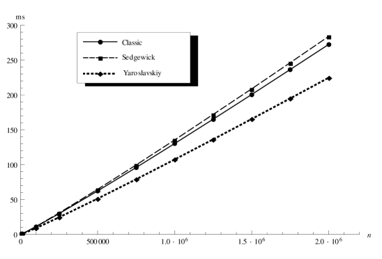
Figure 2: Running times of Java implementations of Algorithms 1, 2 and 3 on an Intel Core 2 Duo P8700 laptop. The plot shows the average running time of 1000 random permutations of each size.

5 Conclusion and Future Work

Having understood how the new Quicksort saves key comparions, there are plenty of future research directions. The question if and how the new Quicksort can compensate for the many extra swaps it needs, calls for further examination. One might conjecture that comparisons have a higher runtime impact than swaps. It would be interesting to see a closer investigation – empirically or theoretically.

In this paper, we only considered the most basic implementation of dual pivot Quicksort. Many suggestions to improve the classic algorithm are also applicable to it. We are currently working on the effect of selecting the pivot from a larger sample and are keen to see the performance impacts.

Being intended as a standard sorting method, it is not sufficient for the new Quicksort to perform well on random permutations. One also has to take into account other input distributions, most notably the occurrence of equal keys or biases in the data. This might be done using Maximum Likelihood Analysis as introduced in [8], which also helped us much in discovering the results of this paper. Moreover, Yaroslavskiy’s partitioning method can be used to improve Quickselect. Our corresponding results are omitted due to space constraints.

Appendix A Solution of the Dual Pivot Quicksort Recurrence

The presented analysis is a generalization of the derivation given by Sedgewick in [11, p. 156ff]. In [5], Hennequin gives an alternative approach based on generating functions that is much more general. Even though the authors consider Hennequin’s method more elegant, we prefer the elementary proof, as it allows a self-contained presentation.

The expected costs $C_{n}$ for sorting a random permutation of length $n$ by any dual pivot Quicksort fulfilling Property 1 satisfy the following recurrence relation (for $n\geq 2$):

$$C_{n} =\sum_{1\leq p<q\leq n}\Pr[\mbox{pivots }(p,q)]\cdot\left(\mbox{partitioning costs}+\mbox{recursive costs}\right)$$

$$=\sum_{1\leq p<q\leq n}\frac{2}{n(n-1)}\left(\mbox{partitioning costs}+C_{p-1}+C_{q-p-1}+C_{n-q}\right)$$

$$=\mathop{\mbox{$\mathbb{E}$}}\nolimits\mbox{partitioning costs}+\frac{2}{n(n-1)}\cdot 3\sum_{k=0}^{n-2}(n-k-1)C_{k}\;.$$

(The last equation follows from splitting up the sum and shifting indices.)
As both algorithms skip subfiles of length $\leq 1$, the base case is $C_{0}=C_{1}=0$.

We will solve this recurrence relation for linear expected partitioning costs $a(n+1)+b$, where $a$ and $b$ are constants depending on the kind of costs we analyze. It turns out that the costs for (sub)lists of length $n=2$ do not fit the linear pattern. Hence, we add $C_{2}=d$ as an additional base case and use the recurrence for $n\geq 3$.

We first consider $D_{n}:=\tbinom{n+1}{2}C_{n+1}-\tbinom{n}{2}C_{n}$ to get rid of the factor in the sum:

$$D{}_{n} =\tbinom{n+1}{2}\bigl{(}a(n+2)+b\bigr{)}-\tbinom{n}{2}\bigl{(}a(n+1)+b\bigr{)}$$

$$\hphantom{\mbox{}=\mbox{}}+\tfrac{(n+1)n}{2}\tfrac{6}{(n+1)n}\sum_{k=0}^{n-1}(n-k)C_{k}-\tfrac{n(n-1)}{2}\tfrac{6}{n(n-1)}\sum_{k=0}^{n-2}(n-k-1)C_{k}$$

$$=3\tbinom{n+1}{2}a+n\cdot b+3\sum_{k=0}^{n-1}C_{k}\;.\qquad\qquad(n\geq 3)$$

The remaining full history recurrence can be solved by taking ordinary differences $E_{n}:=D_{n+1}-D_{n}=3(n+1)a+b+3C_{n}$ for $n\geq 3$. Using the definition of $E_{n}$ and some tedious, yet elementary rearrangements we find

$$\left(E_{n}-3C_{n}\right)\bigm{/}\tbinom{n+2}{2}=C_{n+2}-\tfrac{2n}{n+2}C_{n+1}+\tfrac{n-3}{n+1}C_{n}\;.$$

Considering yet another quantity $F_{n}:=C_{n}-\frac{n-4}{n}\cdot C_{n-1}$, one easily checks that $F_{n+2}-F_{n+1}=C_{n+2}-\tfrac{2n}{n+2}C_{n+1}+\tfrac{n-3}{n+1}C_{n}$ holds, such that we conclude

$$F_{n+2}-F_{n+1}=\left(E_{n}-3C_{n}\right)\bigm{/}\tbinom{n+2}{2}=\bigl{(}3(n+1)a+b\bigr{)}\bigm{/}\tbinom{n+2}{2}\;.\qquad(n\geq 3)$$

This last equation is now amenable to simple iteration:

$$F_{n} =\sum_{i=5}^{n}\bigl{(}3(i-1)a+b\bigr{)}\bigm{/}\!\tbinom{i}{2}+F_{4}$$

$$=\sum_{i=5}^{n}\frac{3(i-1)a}{\frac{1}{2}i(i-1)}+\sum_{i=5}^{n}\frac{b}{\frac{1}{2}i(i-1)}+F_{4}$$

$$=6a\sum_{i=5}^{n}\tfrac{1}{i}+2b\sum_{i=5}^{n}\left(\tfrac{1}{i-1}-\tfrac{1}{i}\right)+F_{4}$$

$$=6a(\mathcal{H}_{n}-\mathcal{H}_{4})+2b\left(\tfrac{1}{4}-\tfrac{1}{n}\right)+F_{4}\;.\qquad(n\geq 5)$$

($\mathcal{H}_{n}:=\sum_{i=1}^{n}\nicefrac{{1}}{{i}}$ is the $n$th harmonic number.)
Plugging in the definition of $F_{n}=C_{n}-\frac{n-4}{n}\cdot C_{n-1}$ yields

$$C_{n}=\tfrac{n-4}{n}\cdot C_{n-1}\;+\;6a(\mathcal{H}_{n}-\mathcal{H}_{4})+2b\left(\tfrac{1}{4}-\tfrac{1}{n}\right)+F_{4}\;.$$

Multiplying by $\tbinom{n}{4}$ and using $\tbinom{n}{4}\cdot\frac{n-4}{n}=\tbinom{n-1}{4}$ gives a telescoping recurrence for $G_{n}:=\tbinom{n}{4}C_{n}$:

$$G_{n} =G_{n-1}\;+\;6a(\mathcal{H}_{n}-\mathcal{H}_{4})\tbinom{n}{4}+2b\left(\tfrac{1}{4}-\tfrac{1}{n}\right)\tbinom{n}{4}+F_{4}\tbinom{n}{4}$$

$$=\sum_{i=5}^{n}\Bigl{[}6a(\mathcal{H}_{i}-\mathcal{H}_{4})\tbinom{i}{4}+2b\left(\tfrac{1}{4}-\tfrac{1}{i}\right)\tbinom{i}{4}+F_{4}\tbinom{i}{4}\Bigr{]}+G_{4}$$

$$=\sum_{i=1}^{n}\Bigl{[}6a(\mathcal{H}_{i}-\mathcal{H}_{4})\tbinom{i}{4}+2b\left(\tfrac{1}{4}-\tfrac{1}{i}\right)\tbinom{i}{4}+F_{4}\tbinom{i}{4}\Bigr{]}\underbrace{-F_{4}\tbinom{4}{4}+G_{4}}_{=0}$$

$$=6a\sum_{i=1}^{n}\mathcal{H}_{i}\tbinom{i}{4}+(\tfrac{1}{2}b-6\mathcal{H}_{4}a+F_{4})\sum_{i=1}^{n}\tbinom{i}{4}-2b\sum_{i=1}^{n}\tfrac{1}{i}\tbinom{i}{4}$$

$$=6a\tbinom{n+1}{5}\left(\mathcal{H}_{n+1}-\tfrac{1}{5}\right)+(\tfrac{1}{2}b-6\mathcal{H}_{4}a+F_{4})\tbinom{n+1}{5}-2b\sum_{i=1}^{n}\tfrac{1}{4}\tbinom{i-1}{3}$$

$$=6a\tbinom{n+1}{5}\left(\mathcal{H}_{n+1}-\tfrac{1}{5}\right)+(\tfrac{1}{2}b-6\mathcal{H}_{4}a+F_{4})\tbinom{n+1}{5}-\tfrac{1}{2}b\tbinom{n}{4}\;.$$

Finally, we arrive at an explicit formula for $C_{n}$ valid for $n\geq 4$:

$$C_{n} =G_{n}\bigm{/}\!\tbinom{n}{4}=\tfrac{6}{5}a\cdot(n+1)\left(\mathcal{H}_{n+1}-\tfrac{1}{5}\right)+(\tfrac{1}{10}b-\tfrac{6}{5}\mathcal{H}_{4}a+\tfrac{1}{5}F_{4})\cdot(n+1)-\tfrac{1}{2}b\;.$$

Using $F_{4}=5a+b+\frac{1}{2}d$, this simplifies to the claimed closed form

$$C_{n}=\tfrac{6}{5}a\cdot(n+1)\left(\mathcal{H}_{n+1}-\tfrac{1}{5}\right)+\bigl{(}-\tfrac{3}{2}a+\tfrac{3}{10}b+\tfrac{1}{10}d\,\bigr{)}\cdot(n+1)-\tfrac{1}{2}b\;.$$

Appendix B Explanation for the Curious $\frac{n-q}{n-2}$ Terms

All Quicksort variants studied in this paper perform partitioning by some variant of Hoare’s “crossing pointers technique”. This technique gives rise to two different cases for “crossing”: As the pointers are moved alternatingly towards each other, one of them will reach the crossing point first – waiting for the other to arrive.

The asymmetric nature of Algorithm 3 leads to small differences in the number of swaps and comparisons in these two cases: If the left pointer $k$ moves last, we always leave the outer loop of Algorithm 3 with $k=g+1$ since the loop continues as long as $k\leq g$ and $k$ increases by one in each iteration. If $g$ moves last, we decrement $g$ and increment $k$, so we can end up with $k=g+2$. Consequently, operations that are executed for every value of $k$ experience one additional occurrence.

To precisely analyze the impact of this behavior, the following equivalence is useful.

Lemma 1.

Let $A[1],\dots,A[n]$ contain a random permutation of $\{1,\dots,n\}$. Then, Algorithm 3 leaves the outer loop with $k=g+2$ (at line 3) iff initially $A[q]>q$ holds, where $q=\max\{A[1],A[n]\}$ is the large pivot.

For conciseness, we will abbreviate “Algorithm 3 leaves the loop with $k=g+i$ ” as “Case $i$ ” for $i=1,2$. Proof: Assume Case 2 occurs, i. e. the loop is left with a difference of 2 between $k$ and $g$. This difference can only show up when both $k$ is inremented and $g$ is decremented. Hence, in the last iteration we must have entered the else-if-branch in line 3 and accordingly $A[k]>q$ must have held there.

Recall that in the end, $q$ is moved to position $g$, so when the loop is left, at line 3 we have $g=q-1$. By assumption, we are in Case 2, so $k=g+2=q+1$ here. As $k$ has been increased once since the last test in line 3, we know that $A[q]>q$, as claimed.

Assume conversely that $A[q]>q$. As $g$ stops at $q-1$ and is always decremented in line 3, we have $g=q$ for the last execution of line 3. By assumption $A[g]=A[q]>q$, so the loop in line 3 must have been left because of a violation of condition “$k<g$”. This implies $k\geq g=q$ in line 3. With the following decrement of $g$ and increment of $k$, we leave the loop with $k\geq g+2$, so we are in Case 2.∎

Lemma 1 immediately implies that Case 2 occurs with probability $\frac{n-q}{n-2}$, given pivots $p$ and $q$: For $q<n$, there are $n-2$ elements that can possibly take position $A[q]$ and $n-q$ of them are $>q$. For $q=n$, we never have $A[q]>q$ and $\frac{n-q}{n-2}=0$. ∎

B.1 Additional Contributions to Comparisons

In Algorithm 3, the comparison in line 3 is executed once for every value of $k$. Hence, we get an additional contribution of one for Case 2. For the conditional expectation $c_{n}^{p,q}$, we get an additional summand $1\cdot\Pr[\mbox{Case 2}]=\frac{n-q}{n-2}$.

Line 3 is reached for every value of $k$ with $A[k]\geq p$. By Lemma 1, Case 2 is equivalent to $A[q]>q>p$, hence the comparison in line 3 is executed exactly once more for $k=q$. This is another contribution of $\frac{n-q}{n-2}$ to $c_{n}^{p,q}$.

Finally, line 3 is executed for all values of $g$ with $A[g]\leq q$ plus one additional time in Case 2: As argued in the proof of Lemma 1, in Case 2, we always quit the last execution of the loop in line 3 because of condition “$k<g$”, as the other condition is guaranteed to hold. Consequently, we get an execution of line 3 for $g=q$ even though $A[g]>q$. This comparison is not accounted for by the terms $\mathop{\mbox{$\mathbb{E}$}}\nolimits\left[s\,@\,\mathcal{G}\,|\,p,q\right]+\mathop{\mbox{$\mathbb{E}$}}\nolimits\left[m\,@\,\mathcal{G}\,|\,p,q\right]$ discussed in the main text. Hence, it entails an additional contribution of $\frac{n-q}{n-2}$ for $c_{n}^{p,q}$

The expected number of executions of line 3, $|\mathcal{G}|$, is not affected by Case 2, so no additional term, here. Summing up, we have $3\cdot\frac{n-q}{n-2}$ additional comparisons that have not been taken into account by the discussion in the main text.

B.2 Additional Contributions to Swaps

Line 3 is executed for values of $k$ with $A[k]<p$. In Case 2, $k$ attains one more value, namely $k=q$. Nevertheless, for this new value of $k$, we do not reach line 3, as Lemma 1 tells us that $A[q]>q>p$.

The swap in line 3 is always followed by line 3, so these lines are visited equally often. As shown above, line 3 causes an additional contribution of $\frac{n-q}{n-2}$.

Finally, the expected number of executions of line 3, $\mathop{\mbox{$\mathbb{E}$}}\nolimits\left[s\,@\,\mathcal{G}\,|\,p,q\right]$, is not affected by Case 2, as $\mathcal{G}$ is the same in Case 1 and 2.

In summary, we find an additional contribution of $\frac{n-q}{n-2}$ to $s_{n}^{p,q}$.

References

- [1] Jon L. Bentley and M. Douglas McIlroy. Engineering a sort function. Software: Practice and Experience, 23(11):1249–1265, 1993.
- [2] Guy E. Blelloch, Charles E. Leiserson, Bruce M. Maggs, C. Greg Plaxton, Stephen J. Smith, and Marco Zagha. A comparison of sorting algorithms for the connection machine CM-2. In Annual ACM symposium on Parallel algorithms and architectures, pages 3–16, New York, USA, June 1991. ACM Press.
- [3] W. D. Frazer and A. C. McKellar. Samplesort: A Sampling Approach to Minimal Storage Tree Sorting. Journal of the ACM, 17(3):496–507, July 1970.
- [4] Pascal Hennequin. Combinatorial analysis of Quicksort algorithm. Informatique théorique et applications, 23(3):317–333, 1989.
- [5] Pascal Hennequin. Analyse en moyenne d’algorithmes : tri rapide et arbres de recherche. PhD Thesis, Ecole Politechnique, Palaiseau, 1991.
- [6] C. A. R. Hoare. Algorithm 63: Partition. Communications of the ACM, 4(7):321, July 1961.
- [7] C. A. R. Hoare. Quicksort. The Computer Journal, 5(1):10–16, January 1962.
- [8] Ulrich Laube and Markus E. Nebel. Maximum likelihood analysis of algorithms and data structures. Theoretical Computer Science, 411(1):188–212, January 2010.
- [9] Nikolaj Leischner, Vitaly Osipov, and Peter Sanders. GPU sample sort. In 2010 IEEE International Symposium on Parallel Distributed Processing IPDPS, pages 1–10. IEEE, 2009.
- [10] Peter Sanders and Sebastian Winkel. Super Scalar Sample Sort. In Susanne Albers and Tomasz Radzik, editors, ESA 2004. LNCS, vol. 3221, pages 784–796. Springer Berlin/Heidelberg, 2004.
- [11] Robert Sedgewick. Quicksort. PhD Thesis, Stanford University, 1975.
- [12] Robert Sedgewick. Quicksort with Equal Keys. SIAM Journal on Computing, 6(2):240–267, 1977.
- [13] Robert Sedgewick. The analysis of Quicksort programs. Acta Inf., 7(4):327–355, 1977.
- [14] Robert Sedgewick. Implementing Quicksort programs. Communications of the ACM, 21(10):847–857, October 1978.