Maximal Rabi frequency of an electrically driven spin in a disordered magnetic field

Abstract

We present a theoretical study of the spin dynamics of a single electron confined in a quantum dot. Spin dynamics is induced by the interplay of electrical driving and the presence of a spatially disordered magnetic field, the latter being transverse to a homogeneous magnetic field. We focus on the case of strong driving, i.e., when the oscillation amplitude $A$ of the electron’s wave packet is comparable to the quantum dot length $L$. We show that electrically driven spin resonance can be induced in this system by subharmonic driving, i.e., if the excitation frequency is an integer fraction (1/2, 1/3, etc) of the Larmor frequency. At strong driving we find that (i) the Rabi frequencies at the subharmonic resonances are comparable to the Rabi frequency at the fundamental resonance, and (ii) at each subharmonic resonance, the Rabi frequency can be maximized by setting the drive strength to an optimal, finite value. In the context of practical quantum information processing, these findings highlight the availability of subharmonic resonances for qubit control with effectivity close to that of the fundamental resonance, and the possibility that increasing the drive strength might lead to a decreasing qubit-flip speed. Our simple model is applied to describe electrical control of a spin-valley qubit in a weakly disordered carbon nanotube.

Introduction. Controlled two-level systems are essential constituents of a number of existing applications including magnetic resonance imaging and atomic clocks, and could form the basis for the potential future technology of quantum information processing. An archetype of controlled two-level systems is the electron spin in the presence of a static magnetic field, illuminated by an ac transverse magnetic fieldShirley (1965); Koppens et al. (2006). If the energy quantum $\hbar\omega$ of the ac field matches the energy distance $\hbar\omega_{L}$ between the two spin levels, then the electron, occupying the ground state before switching on the radiation, will evolve coherently and cyclically between the ground and excited spin states. This dynamics is known as Rabi oscillation, and the inverse time scale of a complete ground state—excited state transition, usually proportional to the amplitude $B_{\rm ac}$ of the ac field, is called the Rabi frequency.

Rabi oscillations can also occur if the energy quantum of the transverse ac field is an integer fraction (subharmonic) of the energy difference between the spin levelsShirley (1965), i.e., if $\hbar\omega=\hbar\omega_{L}/N$ with $N\in\mathbb{Z}^{+}$. As long as the spin splitting $\hbar\omega_{L}$ dominates the amplitude $B_{\rm ac}$ of the transverse field, the Rabi frequency $\Omega^{(N)}$ of the $N$th subharmonic transition (a.k.a. the $N$-photon transition) shows the dependence $\Omega^{(N)}\propto B_{\rm ac}\left(\frac{B_{\rm ac}}{\hbar\omega_{L}}\right)^{(N-1)}$, meaning that (i) a higher $N$ implies a slower Rabi oscillation, and (ii) the Rabi frequency increases when $B_{\rm ac}$ is increased.

Subharmonic spin resonances have recently been observedLaird et al. (2009); Schroer et al. (2011); Nadj-Perge et al. (2012); Pei et al. (2012); Laird et al. (2013) in electrically driven quantum dots (QDs)Nowack et al. (2007); Laird et al. (2007); Pioro-Ladriere et al. (2008); Golovach et al. (2006); Flindt et al. (2006). In these systems, electrical driving might be favorable over magnetic excitation, as the former allows for selective addressing of spin-based quantum bits in a multi-quantum-dot register. The ac electric field induces an oscillatory motion of the electron in the QD, which in turn gives rise to spin rotations, provided that a suitable interaction between spin and motion is present in the sample. Examples are spin-orbit and hyperfine interactions, and spatially dependent magnetic fields. Theory works have addressed subharmonic EDSR (electrically driven spin resonance) assisted by $g$-tensor modulation for donor-bound electronsDe et al. (2009) and holes in self-assembled QDs Pingenot et al. (2011), and by nonlinear charge dynamics in a double-dot potentialRashba (2011). References Nowak et al., 2012; Osika et al., 2013 analyzed subharmonic transitions via numerical simulations of EDSR in nanowire QDs.

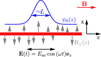
Figure 1: (Color online) A simple model for electrically driven spin resonance. An electron confined to a quantum dot in a nanowire, subject to a static homogeneous $B$-field and a spatially inhomogeneous, disordered transverse magnetic field (represented by the gray vertical arrows) is shaken by the ac $E$-field $\mathbf{E}(t)$.

In this work, we consider a practically relevant, yet simple model of EDSR. In this model, a single electron occupies a one-dimensional (1D) parabolic QD, subject to a homogeneous static magnetic field $\mathbf{B}$, an inhomogeneous, disordered transverse magnetic field $\mathbf{B}_{\perp}(z)\perp\mathbf{B}$, and an ac driving electric field $\mathbf{E}(t)$ (see Fig. 1). We focus on the regime of strong driving, when the amplitude $A$ of the electron’s spatial oscillations, induced by the ac electric field, is comparable to the length $L$ of the QD. We show that EDSR can be induced in this system by subharmonic driving, i.e., if the excitation frequency $\omega$ is an integer fraction (1/2, 1/3, etc) of the Larmor frequency $\omega_{L}$. At strong driving we find that (i) the Rabi frequencies at the subharmonic resonances are comparable to the Rabi frequency of the fundamental resonance, and (ii) at each subharmonic resonance, the Rabi frequency can be maximized by setting the drive strength to an optimal finite value. Finally, our model is used to describe electrical control of a spin-valley qubit in a disordered carbon nanotube (CNT).

The motivation for this study is threefold. (1) Speed of manipulation is a central quantity in practical quantum information processing. It is tempting to believe that in EDSR, a stronger electric drive implies faster spin manipulation; in fact, we are unaware of any theoretical or experimental results indicating deviations from this relation. Our present study of the strong-driving regime allows us to reconsider (and refute) this expectation, and to estimate the drive strength allowing for the fastest spin control achievable in the strong-driving regime. (2) Nonlinear processes arising from the interaction of matter and electromagnetic fields are fundamentally important and have found a wide range of applications in nonlinear optics as well as in nanoelectronics. Subharmonic EDSR is a distinct example of such nonlinear processes, and might gain importance as a mechanism of nonlinear interaction between single-spin QDs and microwave nanocircuitsTrif et al. (2008); Petersson et al. (2012). (3) In a recent experiment using a CNT QDLaird et al. (2013), the strong-driving regime of EDSR has been achieved: the authors estimatedNot a maximum electric-field amplitude of $E_{\rm ac}\approx 4\times 10^{4}\ {\rm V}/{\rm m}$ , QD length $L\approx 100$ nm, and level spacing $\hbar\omega_{0}\approx 3$ meV, implying a ratio $A/L\approx 1.3$ at maximum drive power. The same group has demonstratedPei et al. (2012) the existence of subharmonic EDSR, up to five-photon transitions, in CNT devices. These experimental findings motivate the study of the strong-driving regime of EDSR.

Model. The static Hamiltonian, describing a single spinful electron in a 1D parabolic QD, is defined as (see Fig. 1).

$$H_{stat}=\frac{p_{z}^{2}}{2m}+\frac{1}{2}m\omega_{0}^{2}z^{2}+\frac{1}{2}B\sigma_{z}+\frac{1}{2}B_{\perp}(z)\sigma_{x},$$ (1)

where $m$ is the effective mass of the electron, $\omega_{0}$ is the angular frequency associated to the harmonic confinement, $B\equiv\hbar\omega_{L}$ [$B_{\perp}(z)$] is the dc homogeneous longitudinal [disordered transverse] magnetic field pointing along the $z$ [$x$] direction, and $\sigma_{x,z}$ are the first and third Pauli matrices representing the electron spin (or pseudospin, see below). The unit matrix in spin space is suppressed. The QD confinement length is $L=\sqrt{\hbar/m\omega_{0}}$.

In practice, the disordered transverse field (DTF) $B_{\perp}(z)$ might be induced by nuclear spins or other short-range impurities. Therefore, we describe the DTF as a sum of Dirac deltas with random prefactors:

$$B_{\perp}(z)=a\sum_{i}\xi_{i}\delta(z-z_{i}),$$ (2)

where $a$ is the lattice constant and $\xi_{i}$ are independent, identically distributed, and zero-mean random variables: $\langle\xi_{i}\rangle=0$ and $\langle\xi_{i}\xi_{j}\rangle=\xi^{2}\delta_{i,j}$. The dimension of $B$, $B_{\perp}$, $\xi_{i}$, and $\xi$ is energy.

The QD spreads over many impurity sites. Therefore, due to the central limit theorem, the matrix elements of the DTF between the harmonic oscillator basis functions $|n\rangle$ ($n\in\mathbb{N}$) are well approximated by zero-mean Gaussian random variables with standard deviation of the order of $\xi\sqrt{\frac{a}{L}}$. To characterize the corresponding energy scale, we introduce $\tilde{B}_{\perp}\equiv\sqrt{\big{\langle}\langle 0|B_{\perp}(z)|0\rangle^{2}\big{\rangle}_{\rm dis}}=\xi\sqrt{\frac{a}{L\sqrt{2\pi}}}$, where $\langle.\rangle_{\rm dis}$ is disorder averaging for the realizations of the $\xi_{i}$’s.

To control the two-level system, we use an oscillating electric field along the nanowire holding the QD:

$$H_{E}=|e|E_{\rm ac}z\cos(\omega t).$$ (3)

We characterize the length scale of this driving by the amplitude $A=|e|E_{\rm ac}L^{2}/\hbar\omega_{0}$ of the center-of-mass oscillations of the electron induced by the electric field. We consider the experimentally motivated energy scale hierarchy

$$\hbar\omega_{0}\gg B\sim\hbar\omega\gg\tilde{B}_{\perp}.$$ (4)

Tool: the co-moving frame. Our goal is to describe the coherent spin dynamics in the strong-driving regime, i.e., when the electric field is strong enough to induce an oscillation amplitude comparable to the confinement length, $A\sim L$. This condition corresponds to the energy-scale relation $|e|E_{\rm ac}L\sim\hbar\omega_{0}$. In this regime, the electric field cannot be treated as a small perturbation compared to the harmonic oscillator level spacing. Instead of using perturbation theory, we transform the Hamiltonian $H=H_{stat}+H_{E}$ into the wave-function basis co-moving with the confinement potentialRashba (2008); San-Jose et al. (2008). This transformation is represented by the time-dependent unitary operator $U(t)=\sum_{n}|n\rangle\langle n(t)|$, where $|n(t)\rangle$ is the $n$-th harmonic oscillator eigenfunction of the instantaneous orbital Hamiltonian $p_{z}^{2}/2m+m\omega_{0}^{2}z^{2}/2+H_{E}(t)$. This transformation approximately decouples the ground-state spin doublet from the excited states, thereby allowing us to analyze the spin dynamics using a $2\times 2$ effective Hamiltonian.

Transformation to the co-moving frame yields the Hamiltonian matrix $H^{\prime}_{nm}=\langle n|\left(UHU^{\dagger}+i\hbar\dot{U}U^{\dagger}\right)|m\rangle$, which we express as

$$H^{\prime}_{nm}=E_{n}(t)\delta_{nm}+\frac{1}{2}B\delta_{nm}\sigma_{z}+\frac{1}{2}\bar{B}^{nm}_{\perp}(t)\sigma_{x}-\varepsilon_{nm}(t).$$ (5)

Here, $E_{n}(t)$ is an electric-field-dependent shift of the orbital energies. The DTF, represented by $\bar{B}_{\perp}^{nm}(t)\equiv\langle n(t)|B_{\perp}(z)|m(t)\rangle$, becomes time dependent after the transformation. The spin-independent last term of Eq. (5) reads as

$$\varepsilon_{nm}(t)=\frac{i\hbar\omega A}{\sqrt{2}L}\sin{\omega t}\left(\sqrt{n}\delta_{n,m+1}-\sqrt{m}\delta_{m,n+1}\right).$$ (6)

In the co-moving frame, we can safely truncate $H^{\prime}$ to the ground-state spin subspace and use the effective spin Hamiltonian $H^{\prime}_{00}$ to describe spin dynamics. It is possible to take into account the coupling of this two-dimensional subspace to higher-lying states via perturbation theory, yielding spin-dependent corrections to $H^{\prime}_{00}$ of the order of $\bar{B}_{\perp}^{01}\varepsilon_{10}/\hbar\omega_{0}\sim\tilde{B}_{\perp}(\omega/\omega_{0})(A/L)$. This implies that it is indeed justified to use $H^{\prime}_{00}$ as the leading-order spin Hamiltonian as long as $A\ll L\omega_{0}/\omega$, which includes the case $A\sim L$ of our interest.

Rabi frequencies. We have concluded that the effective spin Hamiltonian is

$$H^{\prime}_{00}=\frac{1}{2}B\sigma_{z}+\frac{1}{2}\bar{B}_{\perp}(t)\sigma_{x},$$ (7)

where $\bar{B}_{\perp}(t)\equiv\langle 0(t)|B_{\perp}(z)|0(t)\rangle$. To express the $N$-photon Rabi frequency, we write $\bar{B}_{\perp}(t)$ in Fourier series:

$$\bar{B}_{\perp}(t) = \hbar\Omega^{(0)}+\sum_{N=1}^{\infty}2\hbar\Omega^{(N)}\cos{\left(N\omega t\right)},$$ (8)

$$\hbar\Omega^{(N)} = \frac{1}{2\pi}\int_{0}^{2\pi}d(\omega t)\bar{B}_{\perp}(t)\cos{\left(N\omega t\right)}.$$ (9)

The Fourier series (8) contains cosine terms only, as $H_{E}(t)$ and hence $\bar{B}_{\perp}(t)$ are even functions of $t$.

In the rotating wave approximationShirley (1965), the $N$-photon Rabi frequency, characterizing the spin-flip rate at driving frequency $\omega=\omega_{L}/N$, is simply given by $|\Omega^{(N)}|$. Recall that $\Omega^{(N)}$ is itself a random variable, as its definition is based on the random variables $\xi_{i}$ building up the DTF. We characterize the typical value of the Rabi frequency by the standard deviation of $\Omega^{(N)}$, that is, $\sigma\left(\Omega^{(N)}\right)\equiv\sqrt{\big{\langle}\left[\Omega^{(N)}\right]^{2}\big{\rangle}_{\rm dis}}$. It can be expressed as

$$\sigma\left(\Omega^{(N)}\right) = \frac{\tilde{B}_{\perp}}{2\pi\hbar}\left[\int_{0}^{2\pi}d\tau\int_{0}^{2\pi}d\tau^{\prime}e^{-\frac{A^{2}}{2L^{2}}(\cos\tau-\cos\tau^{\prime})^{2}}\right.$$ (10)

$$\times \left.\cos{(N\tau)}\cos{(N\tau^{\prime})}\right]^{1/2}.$$

From now on, we refer to the typical Rabi frequency simply as the ‘Rabi frequency’.

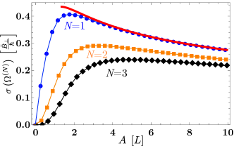
Figure 2: (Color online) The $N$-photon Rabi frequencies for $N=1,2,3$, as functions of the oscillation amplitude of the electronic wavefunction. Thick red line: the $A\gg L$ asymptote, Eq. (11).

In Fig. 2, we plot the $N$-photon Rabi-frequencies, obtained by numerically integrating (10), as a function of the oscillation amplitude $A$ of the electron wave packet. The main features in Fig. 2 are as follows. (i) In the weak-driving regime $A\ll L$, the $N$-photon Rabi frequencies are proportional to $A^{N}\propto E_{\rm ac}^{N}$. This is consistent with perturbation theory. The asymptote of (10) corresponding to this case is $\sigma\left(\Omega^{(N)}\right)\approx\frac{\tilde{B}_{\perp}}{\hbar}\frac{A^{N}}{L^{N}}\sqrt{\frac{(2N)!}{(2^{N}N!)^{3}}}$. (ii) In the regime $A\gtrsim L$, the Rabi frequencies of the subharmonic resonances $N=2,3$ are comparable to the Rabi frequency of the fundamental resonance $N=1$. This is in sharp contrast to the behavior in the weak-driving regime. (iii) Each Rabi-frequency curve has a maximum in the regime $A\sim L$, with the maximum points shifting to larger amplitudes $A$ as the photon number $N$ is increased. (iv) After reaching their maxima, the Rabi frequencies decay if the drive strength is increased to the $A>L$ regime. The asymptote of (10) for the case $N=1$ and $A\gg L$ reads as

$$\sigma\left(\Omega^{(1)}\right)\approx\frac{\tilde{B}_{\perp}}{\hbar}\sqrt{\frac{L}{A}}\left[\left(C^{(1)}_{1}+C^{(1)}_{2}\ln{\frac{A}{L}}\right)\right]^{1/2},$$ (11)

where $C^{(1)}_{1}=\frac{7\ln{2}-4+\gamma}{\sqrt{2\pi^{3}}}\approx 0.18$ and $C^{(1)}_{2}=\sqrt{\frac{2}{\pi^{3}}}\approx 0.25$, where $\gamma\approx 0.58$ is the Euler-Mascheroni constant. The asymptotic result (11) is shown as the red line in Fig. 2.

A simple interpretation of the decaying trend (iv) of the Rabi frequencies for $A\gg L$ can be given using the simplified example of a zigzag-like driving electric field. To this end, we replace the harmonic driving $H_{E}\propto\cos\omega t$ by $H_{E}=|e|E_{\rm ac}zf(t)$ with $f(t)$ being a piecewise linear function of time, decreasing from 1 to -1 (increasing from -1 to 1) in the first (second) half of the period. For this $f(t)$, the center of the electronic wave function moves with constant velocity between turning points, hence it sweeps through any $L$-long segment of its orbit in time $\Delta t=\pi L/2A\omega$. First, this implies that Eq. (9) can be approximated by (for the case $N=1$)

$$\hbar\Omega^{(1)}\approx\frac{1}{2}\frac{L}{A}\sum_{j=0}^{{\rm floor}(2A/L)}\bar{B}_{\perp}(j\Delta t)\cos(\omega j\Delta t).$$ (12)

Second, it implies that it is reasonable to approximate the correlation time of $\bar{B}_{\perp}(t)$ with $\Delta t$; i.e., for $j\neq j^{\prime}$, the distance between the center of the electronic wave function at time $j\Delta t$ and $j^{\prime}\Delta t$ is at least $L$, hence the corresponding values of $\bar{B}_{\perp}$ can be regarded as uncorrelated: $\langle\bar{B}_{\perp}(j\Delta t)\bar{B}_{\perp}(j^{\prime}\Delta t)\rangle_{\rm dis}\propto\delta_{j,j^{\prime}}$. Since the terms of the sum in Eq. (12) are uncorrelated, the standard deviation of the sum varies with $A$ as $\sqrt{A/L}$, hence the standard deviation of the Rabi frequency obeys $\sigma\left(\Omega^{(1)}\right)\propto\sqrt{L/A}$. Although the logarithmic correction obtained in Eq. (11) is absent in the case of this slightly modified driving profile $f(t)$, the decaying trend of the Rabi frequency with growing amplitude $A$ is indeed reproduced.

An important practical consequence of the results shown in Fig. 2 is the following. If the fundamental or a subharmonic resonance is exploited with the aim of fast qubit control, then it is not desirable to increase the amplitude $E_{\rm ac}$ of the driving electric field as much as possible. Instead, there exists an optimal, finite value of $E_{\rm ac}$, of the order of $\hbar\omega_{0}/|e|L$, which maximizes the spin-flip rate for the given resonance.

Two-component DTF. The results obtained from our simple model (1), where the DTF has only one Cartesian component ($x$), can be easily generalized to the case where the DTF has two components ($x$,$y$) transverse to the dc B-field. Then, the DTF Hamiltonian reads $\frac{1}{2}\mathbf{B_{\perp}}(z)\boldsymbol{\sigma}$, where $\boldsymbol{\sigma}=(\sigma_{x},\sigma_{y},\sigma_{z})$, $\mathbf{B}_{\perp}(z)=a\sum_{i}\boldsymbol{\xi}_{i}\delta(z-z_{i}),$ and $\boldsymbol{\xi}_{i}=(\xi_{i,x},\xi_{i,y},0)$. Furthermore, $\langle\xi_{i,\alpha}\rangle_{\rm dis}=0$ and $\langle\xi_{i,\alpha}\xi_{j,\beta}\rangle_{\rm dis}=\delta_{i,j}\delta_{\alpha,\beta}\xi^{2}/2$, with $\alpha,\beta\in\{x,y\}$. In this case of two-component DTF, the effective spin-driving field can be described by complex Fourier coefficients:

$$\Omega^{(N)}=\frac{1}{h}\int_{0}^{2\pi}d(\omega t)\langle 0(t)|B_{\perp,x}(z)+iB_{\perp,y}(z)|0(t)\rangle\cos{(N\omega t)}.$$ (13)

We identify the typical Rabi frequency with $\sigma\left(\Omega^{(N)}\right)=\sqrt{\langle\left|\Omega^{(N)}\right|^{2}\rangle_{\rm dis}}$. With these new definitions, it is straightforward to show that the previously obtained results such as Eq. (10) and Fig. 2 remain valid for the case of a two-component DTF.

Application: coherent control of a spin-valley qubit in a disordered CNT. We show that the simple model developed above is applicable to describe the electrically driven dynamics of a spin-valley qubit in a disordered CNT. Electrically induced qubit rotation in a similar system was observedLaird et al. (2013), and it was attributed to the bent geometryFlensberg and Marcus (2010) of the sample; in contrast, following we describe an alternative mechanism that is active even in a straight CNT.

A simple model Hamiltonian of a single-electron parabolic QD in a weakly disordered CNT in the presence of an external magnetic field $\boldsymbol{\mathcal{B}}=(\mathcal{B}_{x},0,\mathcal{B}_{z})$ reads as

$$H_{\rm CNT} = \frac{p_{z}^{2}}{2m}+\frac{1}{2}m\omega_{0}^{2}z^{2}-\frac{\Delta_{\rm so}}{2}s_{z}\tau_{3}+\frac{1}{2}\mathbf{b}(z)\boldsymbol{\tau}$$ (14)

$$+ \frac{1}{2}g_{\rm s}\mu_{B}\left(\mathcal{B}_{x}s_{x}+\mathcal{B}_{z}s_{z}\right)+\frac{1}{2}g_{\rm orb}\mu_{B}\mathcal{B}_{z}\tau_{3}.$$

The terms of $H_{\rm CNT}$ are, respectively: electronic kinetic energy of the motion along the CNT axis ($z$); parabolic confinement along $z$; spin-orbit interaction characterized by the spin-orbit energy $\Delta_{\rm so}$; valley-mixing short-range potential disorder with $\mathbf{b}(z)=(b_{1}(z),b_{2}(z),0)$; spin Zeeman effect; and orbital Zeeman effect. Furthermore, $m$ is the electronic effective mass, $\mathbf{s}=(s_{x},s_{y},s_{z})$ [$\boldsymbol{\tau}=(\tau_{1},\tau_{2},\tau_{3})$] is the vector of Pauli matrices in the spin [valley] space spanned by $|\!\uparrow\rangle$ and $|\!\downarrow\rangle$ [$|K\rangle$ and $|K^{\prime}\rangle$], and $g_{\rm s}$ ($g_{\rm orb}$) is the spin (orbital) g-factor. Identity matrices in spin and valley space are omitted.

The valley-mixing part of $H_{\rm CNT}$, describing short-range disorder reads $\mathbf{b}(z)=\frac{\Omega_{\rm cell}}{4R\pi}\sum_{i}\boldsymbol{\xi}_{i}\delta(z-z_{i})$, where $\Omega_{\rm cell}$ is the unit cell area of the graphene lattice, $R$ is the CNT radius, and $\boldsymbol{\xi}_{i}=(\xi_{i,1},\xi_{i,2},0)$ is a vector representing the impurity site $i$: $|\boldsymbol{\xi}_{i}|$ is the random on-site energy on the impurity site, and the direction of $\boldsymbol{\xi}_{i}$ is set by the location of the impurity along the CNT circumference Pályi and Burkard (2010, 2011). Potential disorder appears in $H_{\rm CNT}$ only via the valley-mixing term $\frac{1}{2}\mathbf{b}(z)\boldsymbol{\tau}$; the valley-independent part is disregarded as it does not influence spin and valley dynamics.

The basis states of the spin-valley qubit are defined as the ground-state doublet $|K\!\uparrow\rangle,|K^{\prime}\!\downarrow\rangle$ of $H_{\rm CNT}$ in the absence of disorder ($\mathbf{b}(z)=0$) and external $B$-field ($\mathcal{B}_{x}=\mathcal{B}_{z}=0$). We describe the dynamics of the spin-valley qubit induced by the simultaneous presence of disorder, external $B$-field and electric driving, the latter being described by $H_{E}$ as defined in Eq. (3). We consider the case when $\hbar\omega_{0}\gg\Delta_{\rm so}$ and $\Delta_{\rm so}$ exceeds the energy scales of disorder ($\sqrt{\langle|\langle 0|b_{1/2}(z)|0\rangle|^{2}\rangle_{\rm dis}}$) and Zeeman splittings in $H_{\rm CNT}$.

We derive an effective $2\times 2$ Hamiltonian for the spin-valley qubit, that is formally identical to Eq. (7). The derivation proceeds as follows. First, we transform the total Hamiltonian $H_{\rm CNT}+H_{E}$ to the co-moving frame of the oscillating electron, as done earlier to obtain Eq. (5). Then, we truncate the Hilbert-space to the four-dimensional subspace corresponding to the ground-state orbital level of the parabolic confinement. Finally, we obtain a $2\times 2$ Hamiltonian for the spin-valley qubit by decoupling its subspace from the subspace of the higher-lying doublet via second-order Schrieffer-Wolff perturbation theory Winkler (2003); Flensberg and Marcus (2010); Széchenyi and Pályi (2013) in the disorder and Zeeman matrix elements. The resulting effective spin-valley qubit Hamiltonian, expressed in the $|K\uparrow\rangle$, $|K^{\prime}\downarrow\rangle$ basis, reads as

$$H_{\rm sv}=\frac{1}{2}(g_{\rm s}+g_{\rm orb})\mu_{B}\mathcal{B}_{z}\sigma_{z}+\frac{1}{2}\frac{g_{\rm s}\mu_{B}\mathcal{B}_{x}}{\Delta_{\rm so}}\langle 0(t)|\mathbf{b}|0(t)\rangle\boldsymbol{\sigma}.$$ (15)

The correspondence between this Hamiltonian and that of Eq. (7) implies that the spin-valley qubit undergoes coherent Rabi oscillations whenever the $N$-photon resonance condition $\hbar\omega N=\mu_{B}(g_{\rm s}+g_{\rm orb})\mathcal{B}_{z}$ is fulfilled. The corresponding Rabi frequency at the $N$-photon resonance is given by Eq. (10) and Fig. 2, with the substitution

$$\tilde{B}_{\perp}\mapsto\frac{g_{\rm s}\mu_{B}\mathcal{B}_{x}}{\Delta_{\rm so}}\sqrt{\frac{\Omega_{\rm cell}}{2(2\pi)^{3/2}RL}}\xi$$ (16)

and $\xi=\sqrt{\langle\boldsymbol{\xi}_{i}^{2}\rangle_{\rm dis}}$. Note that Eq. (10) and Fig. 2 apply in this case only if the counterpart of the condition (4) is fulfilled, i.e., if $\mu_{B}(g_{\rm s}+g_{\rm orb})B_{z}$ exceeds $\tilde{B}_{\perp}$, the latter being defined by Eq. (16).

For the realistic parameter set $R=1$ nm, $L=100$ nm, $\xi=22$ meV (e.g., 50 impurity sites within the QD, each with a random $\pm 0.5$ eV on-site energy), $\mathcal{B}_{x}=50$ mT, $\mathcal{B}_{z}=10$ mT, $g_{\rm s}=2$, $g_{\rm orb}=50$, and $\Delta_{\rm so}=0.5$ meV, the single-photon resonance frequency is $\omega\approx 46$ GHz, and the maximal Rabi frequency at the single-photon resonance is $\sigma\left(\Omega^{(1)}\right)\approx 0.63$ GHz.

Finally, we point out that our 1D and 2D DTF models are also applicable to describe strongly driven EDSR of heavy holes in semiconductors in the presence of Ising-type hyperfine interactionFischer et al. (2008), and electrically driven valley resonance in CNTsPályi and Burkard (2011), respectively.

Note added: A recent experimentStehlik et al. revealed strong subharmonic resonances in EDSR, similar to those predicted in this work, but presumably caused by a different mechanism (Landau-Zener transitions).