I₂ molecule for neutrino mass spectroscopy: ab initio calculation of spectral rate

Abstract

It has recently been argued that atoms and molecules may become good targets of determining neutrino parameters still undetermined, if atomic/molecular process is enhanced by a new kind of coherence. We compute photon energy spectrum rate arising from coherent radiative neutrino pair emission processes of metastable excited states of I₂ and its iso-valent molecules, $|Av\rangle\rightarrow|Xv^{\prime}\rangle+\gamma+\nu_{i}\nu_{j}$ and $|A^{\prime}v\rangle\rightarrow|Xv^{\prime}\rangle+\gamma+\nu_{i}\nu_{j}$ with $\gamma$ an IR photon and $\nu_{i(j)}$ $i(j)-$th neutrino mass eigenstates, and show how fundamental neutrino parameters may be determined. Energies of electronically excited states of I₂, including the effect of spin-orbit couplings were calculated by the multiconfigurational second order perturbation (CASPT2) method. Summation over many vibrational levels of intermediate states is fully incorporated. Unlike atomic candidate of a much larger energy difference such as Xe, I₂ transitions from a vibrational level $A(v=0)$ to $X(v^{\prime}=24)$ give an opportunity of determination of the mass type (Majorana vs Dirac distinction) and determination of Majorana CPV (charge-conjugation parity violating) phases, although the rate is much smaller.

xxxx, xxx

1 Introduction

Neutrinos are most common particles next to 3 K photons in the present universe, yet their properties eluded comprehensive experimental determination since these neutral particles have only weak interaction. The conventional target for exploration of neutrino properties has been nuclei; stable nuclei in neutrino oscillation experiments and unstable nuclei in other neutrino experiments. Measured quantities derived so far by neutrino oscillation experiments are mass squared differences ($\Delta m_{ij}^{2}\equiv m_{i}^{2}-m_{j}^{2}$) and mixing angles summarized neutrino_2012_a by

$$\Delta m_{21}^{2}\sim 7.5\times 10^{-5}\ \text{eV}^{2}\,,\hskip 14.22636pt|\Delta m_{31}^{2}|\sim 2.5\times 10^{-3}\ \text{eV}^{2}\,,$$ (1)

$$\sin^{2}\theta_{12}\sim 0.31\,,\hskip 14.22636pt\sin^{2}\theta_{23}\sim 0.42\,,\hskip 14.22636pt\sin^{2}\theta_{13}\sim 0.024\,.$$ (2)

It has been assumed in this analysis that there exist only three kinds of neutrino, which we also follow throughout this work. The other hint on the absolute mass scale is derived from cosmological arguments, giving $\sum_{i}m_{i}<O(0.5)$ eV cosmological_bound . The important quantities undetermined in oscillation experiments are (1) absolute neutrino masses (impossible to determine in oscillation experiments), (2) CP symmetry (C=charge conjugation, P = parity) violating phase (CPV phase in short), and (3) whether the massive neutrino belongs to the Majorana type majorana or not.

There are two different kinds of ongoing experiments using unstable nuclei for measurements of still undetermined neutrino parameters; (1) the end point spectrum of beta decay of nuclei such as tritium for the measurement of an averaged absolute neutrino mass value, and (2) the search of neutrino-less double beta decay for verification of lepton number violation related to a finite Majorana type of masses. So far negative limits have been set in these experiments. The reason for the use of unstable nuclei is that the weak decay rate such as the nuclear beta decay increases with a high positive power of the released energy, usually 5th power, and the available nuclear energy of a few MeV gives a detectable rate. But with the expected small neutrino mass of a fraction of eV the energy mismatch becomes a serious problem, and the determination of the absolute neutrino mass value and exploration of undetermined important neutrino properties are more and more difficult.

With the advent of remarkable technological innovations manipulation of atoms and molecules may contribute greatly to fundamental physics. Neutrino physics may also be one of these areas. Atoms and molecules are target candidates of precision neutrino mass spectroscopy, as recently emphasized in Ref. ptep_overview , due to closeness of the energy released in their transition to expected neutrino masses. The relevant process of our interest is cooperative (and coherent, called macro-coherent subsequently) atomic de-excitation; $|e\rangle\rightarrow|g\rangle+\gamma+\nu_{i}\nu_{j}$ where $\nu_{i(j)},i(j)=1,2,3$ is one of neutrino mass eigenstates. $\gamma$ in the present work refers to a photon in the visible to the infrared region. The initial state $|e\rangle$ must be metastable, say its lifetime $\gtrsim O(1)$ msec. The process, as shown in Fig. 1, exists as a combined effect of second order in Quantum Electro-Dynamics (QED) and weak interaction of the standard electroweak theory weak .

To obtain a measurable rate of the process, it is crucial to develop the macro-coherence psr_dynamics ; ptep_overview , a new kind of coherence. The macro-coherent emission of radiative neutrino pairs is stimulated by two trigger irradiation of frequencies $\omega,\omega^{\prime}$ constrained by $\omega+\omega^{\prime}=\epsilon_{eg}/\hbar\,,\omega<\omega^{\prime}$, with $\epsilon_{eg}=\epsilon_{e}-\epsilon_{g}$ the energy difference of initial and final states. The measured photon energy in the de-excitation is given by the smaller frequency $\omega$. The macro-coherence assures that the three-body process, $|e\rangle\rightarrow|g\rangle+\gamma+\nu_{i}\nu_{j}$, conserves both the energy and the momentum. Assuming that atoms in the states $|e\rangle$ and $|g\rangle$ can be taken infinitely heavy and the atomic recoil may be ignored, there exist threshold photon energies nu_observables_1 at

$$\hbar\omega_{ij}=\frac{\epsilon_{eg}}{2}-\frac{(m_{i}c^{2}+m_{j}c^{2})^{2}}{2\epsilon_{eg}}\,.$$ (3)

Each time the emitted photon energy decreases below a fixed threshold energy of $\hbar\omega_{ij}$, a new continuous spectrum is opened, hence there are six energy thresholds $\hbar\omega_{ij}\,,i,j=1,2,3$ ($(i,j)$ threshold for brevity) separated by finite photon energies. Determination of the threshold location given by Eq. (3), hence decomposition into six mass thresholds, is made possible by precision of irradiated laser frequencies at $\omega\approx\omega_{ij}$ and not by resolution of detected photon energy.

The macro-coherently amplified radiative emission of neutrino pair has been called RENP (radiative emission of neutrino pair) ptep_overview , which is the core idea of our neutrino mass spectroscopy that may determine all unknown neutrino parameters. It has been argued that this method using atoms and molecules is ultimately capable of determining the nature of neutrino masses, Dirac vs Majorana distinction and measuring the new Majorana source of CPV phases nu_observables_1 ; nu_observables_2 . It is crucial for explanation of the matter-antimatter asymmetry of the universe to verify the Majorana nature of neutrinos and determine CPV phases related to the Majorana case fy-86 ; davidson-ibarra .

There is an important constraint on possible target atoms/molecules to obtain reasonable rates for realistic experiments. The atomic operator involved in RENP has the character of M1$\times$E1 where the M1 operator (actually electron spin $\vec{S}$ in subsequent RENP formulas) governs the weak interaction Hamiltonian of neutrino pair emission and the E1 operator denotes the usual dipole interaction of QED. The total angular momentum change via virtual intermediate state requires that the $LS$ coupling scheme should be broken ptep_overview , hence candidates should be sought in heavy atoms/molecules. This way we found Xe atom as a good candidate.

Xe atom is excellent, having a great discovery potential of RENP process, and further expected to determine the absolute neutrino mass scale and distinguish the normal mass vs the inverted mass hierarchy (denoted by NH and IH respectively) ptep_overview . On the other hand, distinction of the mass type (Dirac vs Majorana) requires a smaller released energy, of order a fraction of 1 eV, as shown in Ref. nu_observables_2 . In the present work we shall study I₂ and its isovalent molecules for this purpose.

Molecules have a number of merits for RENP: (1) homo-nuclear diatomic molecules such as I₂ have vibrational states among which the usual E1 transition (its Hamiltonian $\propto\vec{d}\cdot\vec{E}$) is forbidden, (2) the richness of vibrational and rotational levels makes it ideal to perform a systematic search of neutrino mass thresholds. Moreover, I₂ molecule has a number of metastable states with energies $\lesssim$ 1 eV above the electronically ground vibrational excited levels.

Electronic excited states of I₂ molecule have been intensively investigated by quantum chemical calculations ISI:A1971J783100039 ; ISI:A1994MW53500001 ; ISI:A1997YJ46400031 . The potential energy curves (PECs) and spectroscopic constants as well as transition properties of this system have been well examined, while the spin operator element which is relevant for the present neutrino mass spectroscopy has not been focused so much. We shall present in this work RENP spectral rate using molecular wave functions based on the first principle calculation.

We show in the present work that the proposed I₂ de-excitation scheme gives a chance of measurements, the Majorana vs Dirac distinction and determination of CPV phases, which are, in the quasi-degenerate case of neutrino masses, easier than NH vs IH distinction at low photon energies where rates are largest. A good sensitivity of the spectral shape to determination of the smallest neutrino mass of order meV is also shown for this target molecule.

Throughout this work we assume that the macro-coherent mechanism as proposed in Ref. ptep_overview . In most of the rest except Sec. 3 where the atomic unit is used following the standard practice of quantum chemistry, we use natural units of $\hbar=1,c=1$.

2 RENP amplitude and rate formula

We shall recapitulate from Ref. ptep_overview main features of the spectral formulas.

The amplitude corresponding to the Feynman-like diagram of Fig. 1 is given by the electroweak theory and reads as

$$\mathcal{M}=G_{F}\vec{E}\cdot\left(\sum_{p}\frac{\langle g|\vec{d}|p\rangle\langle p|\vec{S}|e\rangle}{\epsilon_{pg}-\omega}+\sum_{q}\frac{\langle q|\vec{d}|e\rangle\langle g|\vec{S}_{|}q\rangle}{\epsilon_{qg}-\omega}\right)\cdot\sum_{ij}a_{ij}\nu_{j}^{\dagger}\vec{\sigma}\nu_{i}\,,$$ (4)

$$a_{ij}=U_{ei}^{*}U_{ej}-\frac{1}{2}\delta_{ij}\,,$$ (5)

where $U_{ei}$ (their relation to necessary mixing angles and CPV phases given in Eq. (18)) is the matrix element of neutrino mixing (expressions in terms of measurable quantities given later), and $\nu_{i}(\vec{p},h)$ the neutrino plane wave function of momentum $\vec{p}$ and helicity $h$ of mass $m_{i}$, $\vec{E}$ the electric field of irradiated trigger laser of frequency $\omega<\epsilon_{eg}/2$, $\vec{S}$ the electron spin operator, and $\vec{d}$ the electric dipole operator. Quantum numbers of states should include all of electronic, vibrational, and rotational ones. The sum over all vibrational modes of intermediate states, $|p\rangle$ and $|q\rangle$, is particularly important for molecules. For simplicity we ignore Hönl-London factor hoenl-london of order unity assuming that rotational degrees of freedom are frozen.

Two terms in bracket of the right hand side of Eq. (4) correspond to two different vertices, weak M1 type of neutrino pair emission (its Hamiltonian $\sim G_{F}\vec{S}\cdot\nu_{j}^{\dagger}\vec{\sigma}\nu_{i}$) and QED E1 transition vertex in the second order perturbation theory as depicted in Fig. 1: the first term of molecular state change of $|e\rangle\rightarrow|p\rangle\rightarrow|g\rangle$ shall be designated by E1$\times$M1 and called (a) in the figure, and the second term of molecular state change of $|e\rangle\rightarrow|q\rangle\rightarrow|g\rangle$ shall be designated by M1$\times$E1 and called (b). Both of states $|p\rangle\,,|q\rangle$ are summed over, since they are virtual intermediate states.

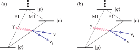
Figure 1: Feynman-like diagrams for RENP from $\Lambda$-type atom/molecule, $|e\rangle\rightarrow|g\rangle+\gamma+\nu_{i}\nu_{j}$, with $\gamma$ a photon and $\nu_{i(j)}$ a neutrino mass eigenstate. Virtual intermediate states $|p\rangle,|q\rangle$ should be summed over. Two-photon transition $|e\rangle\rightarrow|g\rangle+\gamma+\gamma$ may also occur via weak M1$\times$ E1 or E1$\times$M1 couplings to $|p\rangle$ or $|q\rangle$.

For isotropic medium without directional alignment by a magnetic field, this amplitude squared gives the basic rate formula (omitting the second contribution $C^{b}(\omega)$ from $|q\rangle$ in Eq. (4)),

$$\Gamma_{\gamma 2\nu}(\omega)=\Gamma_{dm}C^{a}(\omega)I(\omega)\,,$$ (6)

$$\Gamma_{dm}=\frac{G_{F}^{2}|\vec{E}|^{2}n^{2}V}{18\pi\bar{\epsilon}^{2}}\,,$$ (7)

$$C^{a}(\omega)=\bar{\epsilon}\,^{4}\sum_{p}\frac{\langle g|\vec{d}|p\rangle\cdot\langle p|\vec{d}|g\rangle\langle e|\vec{S}|p\rangle\cdot\langle p|\vec{S}|e\rangle}{(\epsilon_{pg}-\omega)^{2}}\,,$$ (8)

$$I(\omega)=\frac{1}{\bar{\epsilon}\,^{2}}\sum_{ij}(B_{ij}I_{ij}(\omega)+\delta_{M}B^{M}_{ij}I^{M}_{ij}(\omega))\theta(\omega_{ij}-\omega)\,,$$ (9)

$$B_{ij}=|a_{ij}|^{2}\,,\hskip 14.22636ptB^{M}_{ij}=\Re(a_{ij}^{2})\,,$$ (10)

$$I_{ij}(\omega)=\Delta_{ij}(\omega)\left(\frac{1}{3}\epsilon_{eg}(\epsilon_{eg}-2\omega)+\frac{1}{6}\omega^{2}-\frac{1}{18}\omega^{2}\Delta_{ij}^{2}(\omega)-\frac{1}{6}(m_{i}^{2}+m_{j}^{2})-\frac{1}{6}\frac{(\epsilon_{eg}-\omega)^{2}}{\epsilon_{eg}^{2}(\epsilon_{eg}-2\omega)^{2}}(m_{i}^{2}-m_{j}^{2})^{2}\right)\,,$$

(11)

$$I^{M}_{ij}(\omega)=-m_{i}m_{j}\Delta_{ij}(\omega)\,,$$ (12)

$$\Delta_{ij}(\omega)=\frac{1}{\epsilon_{eg}(\epsilon_{eg}-2\omega)}\left\{\left(\epsilon_{eg}(\epsilon_{eg}-2\omega)-(m_{i}+m_{j})^{2}\right)\left(\epsilon_{eg}(\epsilon_{eg}-2\omega)-(m_{i}-m_{j})^{2}\right)\right\}^{1/2}\,.$$ (13)

In the overall rate factor $\Gamma_{dm}$ for diatomic molecules the directionality of trigger correlated with the molecular axis is taken into account by an extra $1/3$ reduction factor. $\bar{\epsilon}$ is a reference energy, to make both $C^{a}(\omega)$ and $I(\omega)$ dimensionless. In the rest of this work we take $\bar{\epsilon}=\epsilon_{eg}$. The function $\theta(x)=0$ for $x<0$, $=1$ for $x>0$ is the step function, giving rise to six mass thresholds in Eq. (9).

$\delta_{M}=1$ for the case of Majorana neutrinos and $\delta_{M}=0$ for the Dirac neutrino. This term $\propto\delta_{M}$ exhibits the quantum mechanical interference intrinsic to identical fermions of Majorana particles nu_observables_1 , which arises from the anti-symmetric wave functions of two identical fermions. For the Dirac neutrino case, emitted particles (except the photon) are a neutrino and an anti-neutrino, two distinguishable particles, and hence the interference terms are absent.

For stored field strength $|\vec{E}|^{2}$ we shall take its maximal value $\epsilon_{eg}n$ with $n$ the number density of excited state targets. More generally, this rate should be multiplied by the dynamical factor $\eta_{\omega}(t)$ whose calculation requires solution of the master equation given in Ref. ptep_overview . It is important to keep in mind that the medium polarization $R_{i}\,,i=1,2$ between $|g\rangle$ and $|p\rangle$ states under trigger irradiation is contained in the dynamical factor given by

$$\eta_{\omega}(t)=\frac{1}{L}\int_{0}^{L}dx\frac{|\vec{E}(x)|^{2}|\langle p|(R_{1}-iR_{2})|g\rangle(x)|^{2}}{4\epsilon_{eg}n^{3}}\,,$$ (14)

an integrated quantity over the entire target at $0\leq x\leq L$ along the trigger irradiation. Thus, a large macroscopic polarization is required for a large RENP rate. The overall maximal rate in the unit of 1/time is

$$\Gamma_{dm}=\frac{G_{F}^{2}n^{3}V}{18\pi\epsilon_{eg}}\sim 26\ \text{kHz}\left(\frac{n}{10^{21}\ \text{cm}^{-3}}\right)^{3}\frac{V}{10^{2}\ \text{cm}^{3}}\frac{0.810\ \text{eV}}{\epsilon_{eg}}\,.$$ (15)

The spectral information is given by $I(\omega)$ which is calculated using neutrino parameters experimentally determined, Eq. (2). Calculation of the molecular factor $C(\omega)$ is the main subject of the next section.

3 Molecular factor

In this section, we investigate the possibility of the RENP experiment using I₂ molecule, with the electronically ground state $X\,0_{g}^{+}$ as the $|g\rangle$ state and the (metastable) electronically excited states $A\,1_{u}$ and $A^{\prime}\,2_{u}$ as the $|e\rangle$ state. An advantage of the $A^{\prime}\,2_{u}$ state over the $A\,1_{u}$ state is its longer natural lifetime. In the simplified model for the RENP process $|A^{\prime}v\rangle\rightarrow|Xv^{\prime}\rangle+\gamma+\nu_{i}\nu_{j}$ in Ref. ptep_overview , only the I₂ $A\,1_{u}$ state is considered as the intermediate $|p\rangle$ state. However, other electronic states may have similar or larger contribution to the molecular factor. We first calculate the molecular factor including several I₂ excited electronic states in the intermediate state summation, without considering vibrational states. There, we examine (1) which intermediate electronic state contributes the most significantly to the molecular factor, (2) relative weight of E1$\times$M1 and M1$\times$E1 amplitude to the RENP process. Second, the effect of nuclear motion (vibrational states) on the molecular factor is investigated considering a single intermediate electronic state, in which we will examine how the molecular factor depends on $(A(v),X(v^{\prime}))$ or $(A^{\prime}(v),X(v^{\prime}))$, a pair of the vibrational states on the $|e\rangle$ and $|g\rangle$ states, which may be useful in designing experiments in future. Finally, the magnitudes of the molecular factor are compared for isovalent molecules, I₂, Br₂ and Cl₂, to study a dependence of the RENP rate on the spin-orbit couplings.

In order to simulate realistic experimental situation, the I₂ energies including the spin-orbit effects are accurately calculated within the framework of the Born-Oppenheimer approximation.

Throughout this section we use atomic units. The conversion factor from the natural unit $C(\omega)$ to the atomic unit $C_{au}(\omega)$ is given by

$$C(\omega)=C_{0}C_{au}(\omega)\,,\hskip 14.22636ptC_{0}=\epsilon_{eg}^{4}\frac{e^{2}a_{0}^{2}}{E_{H}^{2}}\sim 3.9\times 10^{-12}\,,$$ (16)

with $\>a_{0}\sim 0.53\times 10^{-8}\ \text{cm}\,,\>E_{H}\sim 27\ \text{eV}\,,\>e^{2}=4\pi\alpha\sim 4\pi/137\,,\>$ and using $\epsilon_{eg}=0.810$ eV. This gives a rate unit $\Gamma_{dm}C_{0}\sim 1.0\times 10^{-7}$ Hz for $n=10^{21}$ cm^-3 and $V=10^{2}$ cm³.

3.1 Detail of the calculation

The electronic excited states of I₂ molecule were calculated by the multiconfigurational second-order perturbation method (CASPT2) ISI:A1996VM76500021 ; ISI:000085902300005 , based on the reference wavefunctions obtained by the state-averaged complete active space self-consistent field (CASSCF) method ISI:A1985AGJ3300004 ; ISI:A1985AJG5000041 with the atomic natural orbital-relativistic correlation consistent (ANO-RCC) all-electron basis set ISI:000220724300003 . The CASSCF method, using a linear combination of configuration state functions to describe electronic wavefunction, is adequate for calculation of electronically excited states with relatively small computational cost. More accurate energies, including dynamic electronic correlation, can be obtained by the CASPT2 method using the second order perturbation to the zero-th order CASSCF wavefunctions. The scalar relativistic effects were introduced at the CASSCF level by keeping the spin-independent (scalar) terms of the two-component reduced Hamiltonian using the 4th order Douglas-Kroll-Hess method ISI:000222680900005 ; ISI:000225440000011 ; ISI:000179042300015 . At this point, the spin-orbit effects are not included in the CASSCF wavefunctions and the CASPT2 energies. The spin-orbit effects were considered by the state-interaction method, where the spin-orbit matrix elements were evaluated between the CASSCF states using the Breit-Pauli operator ISI:000165193700015 , while the unperturbed diagonal energies were replaced by the CASPT2 energies. Final energies are obtained by diagonalization of this spin-orbit Hamiltonian. Our procedure is very similar to that employed in the calculation of the I₂ potential energy curves by Malmquist et al. ISI:000175958700011 . The D_2h symmetry was employed in our calculations. In the CASSCF calculation, total of 28 orbitals, 1–7$a_{g}$(i.e. $1a_{g},2a_{g},\cdots,7a_{g}$), 1–3$b_{3u}$,1–3$b_{2u}$,1$b_{1g}$,1–7$b_{1u}$,1–3$b_{2g}$,1–3$b_{3g}$ and 1$a_{u}$, were kept doubly occupied. In addition, the 1$a_{g}$ (1$\sigma_{g}$) and 1$b_{1u}$ (1$\sigma_{u}$) orbitals were frozen during the calculation. The remaining 50 electrons were distributed over 26 active orbitals: 8–13$a_{g}$,4–6$b_{3u}$,4–6$b_{2u}$,2$b_{1g}$,8–13$b_{1u}$,4–6$b_{2g}$,4–6$b_{3g}$ and 2$a_{u}$. The state-averaging was performed over 18 electronic states: the three lowest $A_{g}$, one $B_{3u}$, one $B_{2u}$, one $B_{1g}$, one $B_{2g}$, one $B_{3g}$ and one $A_{u}$ states with singlet spin multiplicity, and one $B_{3u}$, one $B_{2u}$, one $B_{1g}$, three $B_{1u}$, one $B_{2g}$, one $B_{3g}$ and one $A_{u}$ states with triplet spin multiplicity. Note that these electronic states correlate with two iodine atoms in the ${}^{2}P$ state at the dissociation limit. By diagonalization of the spin-orbit Hamiltonian, total of 36 spin-orbit eigenstates were obtained. All these calculations were performed using the MOLPRO suite of programs MOLPRO . Although the electric transition dipole moments between the spin-orbit eigenstates were obtained as part of the spin-orbit calculation in the MOLPRO programs, the matrix elements of the electronic spin operator $S$ were not provided. Thus, we explicitly evaluated the spin matrix elements between the spin-orbit eigenstates using the output of the eigenvectors.

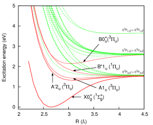
Figure 2: Potential energy curves of I₂ electronic states. The electronic states relevant to this work are indicated by solid red lines.

The potential energy curves of the calculated I₂ electronic states are shown in Fig. 2. In the figure, the spin-orbit eigenstates are correlated with pairs of the atomic states I$({}^{2}P_{3/2})+$I$({}^{2}P_{3/2})$, I$({}^{2}P_{1/2})+$I$({}^{2}P_{3/2})$ or I$({}^{2}P_{1/2})+$I$({}^{2}P_{1/2})$, as the inter-nuclear distance becomes large. The dissociation and excitation energies of the electronic states relevant to this work, as well as the vibrational energies on these states are summarized in Table 1. For the purpose of this work, our results agree well with the experimental values.

Table 1: Calculated vertical and adiabatic ($T_{e}$) excitation energies, dissociation energies ($D_{e}$) and vibrational energies ($\omega_{e}$) for the I₂ $X$, $A^{\prime}$, $A$, $B^{\prime\prime}$ and $B$ states. Experimental values are indicated in parentheses. ^aReference ISI:A1984SD76100008 . ^bReference ISI:A1973P432700019 . ^cReference ISI:A1982PR16400007 . ^dReference ISI:A1981LN51200007 . ^eUnbound in the calculated result. ^fReference ISI:A1985AHT6800017 . ^gReference ISI:A1982NP92500011 . ^hReference ISI:A1986A595600008 .

State	Vertical excitation energies (eV)	$T_{e}$ (eV)	$D_{e}$ (eV)	$\omega_{e}$ (cm-1)
${X}0_{g}^{+}({}^{1}\Sigma^{+}_{g})$	0.0	0.0	1.53 (1.55)a	220.1 (214.5)a
${A^{\prime}}2_{u}({}^{3}\Pi_{u})$	1.88 (1.69)b	1.32 (1.245)c	0.21 (0.311)c	95.3 (108.8)c
${A}1_{u}({}^{3}\Pi_{u})$	1.94 (1.84)b	1.42 (1.353)d	0.11 (0.203)d	77.5 (88.3)d
${B^{\prime\prime}}1_{u}({}^{1}\Pi_{u})$	2.57 (2.49)b	$-$e (1.534)f	$-$e (0.022)f	$-$e (19.8)f
${B}0_{u}^{+}({}^{3}\Pi_{u})$	2.59 (2.37)g	2.14 (1.955)h	0.44 (0.543)h	117.2 (125.7)h

3.2 Molecular factor with the fixed-nuclei approximation

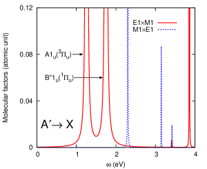
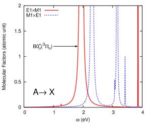
Figure 3: Molecular factors evaluated at $R$ = 2.9 Å. The left panel: the $A^{\prime}$ state was used as the $|e\rangle$ state. The right panel: the $A$ state was used as the $|e\rangle$ state. The red line (E1$\times$M1, corresponding to Fig. 1 (a)) represents molecular factor $C^{a}_{au}=C^{a}/C_{0}$ in Eq. (8). The blue dashed line (M1$\times$E1, corresponding to Fig. 1 (b)) represents molecular factor $C^{b}_{au}=C^{b}/C_{0}$ in Eq. (17).

In this work, we consider the I₂ $A\ 1_{u}({}^{3}\Pi_{u})$ and $A^{\prime}\ 2_{u}({}^{3}\Pi_{u})$ states as $|e\rangle$ state and the $X0_{g}^{+}({}^{1}\Sigma^{+}_{g})$ ground state as $|g\rangle$ state, where electric dipole transition between $|e\rangle$ and $|g\rangle$ is forbidden or only weakly allowed. In order to inspect which I₂ electronic states contribute to the RENP rate as the intermediate $|p\rangle$ state, we calculated $C_{au}(\omega)$ at the fixed inter-nuclear distance of 2.9 Å, which is located between the equilibrium points of the $X$ and $A$/$A^{\prime}$ states, without considering rovibrational energies. All calculated spin-orbit eigenstates are included as intermediate $|p\rangle$ states in evaluating molecular factor $C_{au}(\omega)$. In Fig. 3, calculated molecular factor $C_{au}^{a}(\omega)$ corresponding to Fig. 1 (a) is shown along with the similar molecular factor $C_{au}^{b}(\omega)$ corresponding to Fig. 1 (b), which has expression similar to Eq. (8) but with spin and dipole operators being swapped as

$$C^{b}(\omega)=\epsilon_{eg}^{4}\sum_{q}\frac{\langle g|\vec{S}|q\rangle\cdot\langle q|\vec{S}|g\rangle\langle e|\vec{d}|q\rangle\cdot\langle q|\vec{d}|e\rangle}{(\epsilon_{qg}-\omega)^{2}}.$$ (17)

We only need energies around 0–0.5 eV in evaluating the RENP rate, although the molecular factors are plotted up to 5 eV in Fig. 3 in order to inspect relative contribution of different intermediate electronic states. At low-energy region below 0.5 eV, the molecular factor for the E1$\times$M1 process is larger than that for the M1$\times$E1 process in both the $A^{\prime}\to X$ and $A\to X$ cases. In other word, the first term in the bracket of Eq. (4) dominates over the second term, which suggests that only the first term should be retained for the RENP using I₂ molecule. In the plots, we can observe several spike-like structures which represent contributions of the intermediate electronic states as labeled in the figure. When the $A\ 1_{u}({}^{3}\Pi_{u})$ state is used as the $|e\rangle$ state, the $B\ 0_{u}^{+}({}^{3}\Pi_{u})$ state predominates among contributions from the other states. On the other hand, when the $A^{\prime}\ 2_{u}({}^{3}\Pi_{u})$ state is used as the $|e\rangle$ state, the $A\ 1_{u}({}^{3}\Pi_{u})$ and $B^{\prime\prime}\ 1_{u}({}^{1}\Pi_{u})$ electronic states are especially important at low energy region relevant to this work, while the other states have negligible contributions.

From here on, only the molecular factor in Eq. (8), which corresponds to the E1$\times$M1 process of Fig. 1 (a), will be evaluated. For the $A\to X$ process, we will consider only the $B$ electronic state as the intermediate electronic state. For the $A^{\prime}\to X$ process, the $A$ electronic state will be mainly considered as the intermediate electronic state, since the contribution of the $A$ state looks larger than the $B^{\prime\prime}$ state in the low energy region. Validity of this approximation, inclusion of only the $A$ electronic state in the $A^{\prime}\to X$ process, will be inspected in the Appendix by comparing amplitudes evaluated by the $A$ intermediate electronic state and by the $B^{\prime\prime}$ intermediate electronic state.

3.3 Molecular factor with vibrational levels on the $X$, $A^{\prime}$, $A$ and $B$ electronic states

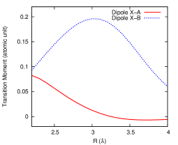
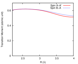
Figure 4: Left panel: Electric dipole transition moment between the $X$ and $A$ states (red solid line), and between the $X$ and $B$ states (blue dashed line). Right panel: Spin transition moment between the $A^{\prime}$ and $A$ states (red solid line), and between the $A$ and $B$ states (blue dashed line).

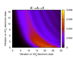
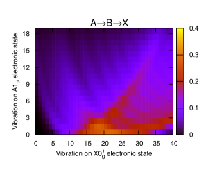
Figure 5: Molecular factor $C_{au}^{a}(\omega)$ at $\omega$ = 0.4 eV, considering vibrational levels on the $X$,$A^{\prime}$,$A$ and $B$ electronic states. The left panel represents the process in which the initial excited electronic state is the $A^{\prime}$ state, the intermediate electronic state is the $A$ state, and the final electronic state is the $X$ state. The right panel represents the process where the initial excited electronic state is the $A$ state, the intermediate electronic state is the $B$ state, and the final electronic state is the $X$ state.

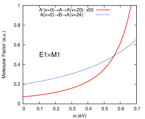
Figure 6: Molecular factor $C_{au}^{a}(\omega)$ as a function of photon energy $\omega$, considering vibrational levels on the $X$,$A^{\prime}$, $A$ and $B$ electronic states.

Since the equilibrium inter-nuclear distances of the $X$ and $A^{\prime}$ states, and of the $X$ and $A$ states are rather different, proper treatment of vibrational wavefunctions may be important to estimate the RENP rate. In this section, we evaluate the molecular factors considering vibrational levels on the $A^{\prime}$, $A$ and $X$ electronic states for the $A^{\prime}\to X$ process, and on the $A$, $B$ and $X$ electronic states for the $A\to X$ process. The ab initio energies of the $X$, $A^{\prime}$, $A$ and $B$ electronic states, the same as shown in Fig. 2, were fitted using the functional form taken from Ref. ISI:A1988R344300002 . The electric dipole transition moment between the $X$ and $A$ states and between the $X$ and $B$ states, the spin transition moment between the $A^{\prime}$ and $A$ states and between the $A$ and $B$ states, shown in Fig. 4, were fitted by polynomial functions. The vibrational energies and wavefunctions on each electronic state were obtained by direct diagonalization of the vibrational Hamiltonian using the pointwise coordinate representation of the wavefunctions, the discrete variable representation (DVR) method colbert1992 , with $R_{min}$ = 2.2 Å, $R_{max}$ = 7.0 Å and $\Delta R$ = 0.006 Å. Summation of the intermediate vibrational states, on the $A$ electronic state in the $A^{\prime}\to X$ process, or on the $B$ electronic state in the $A\to X$ process, was taken up to $v$ = 40. These parameters for the DVR basis and the number of vibrational states in the summation were sufficient to obtain converged result.

In Fig. 5, the calculated molecular factors at $\omega$ = 0.4 eV for the $A^{\prime}\to A\to X$ process and for the the $A\to B\to X$ process are shown as functions of the vibrational levels on the initial ($A^{\prime}$ or $A$) and the final ($X$) electronic states. In the $A^{\prime}\to A\to X$ process shown in the left panel in Fig. 5, the molecular factor is the largest around the point $(A^{\prime}(v=0),X(v^{\prime}=20))$. Starting from this point, the higher intensity region extends to the upper left direction. In the $A\to B\to X$ process shown in the right panel in Fig. 5, the molecular factor is the largest around the point $(A(v=0),X(v^{\prime}=24))$. In this case, the higher intensity region extends to the upper right direction. The structure of these higher intensity regions reflects the fact that the equilibrium points of the $X$ and $A^{\prime}$ (or $A$) states are separated, and one of or both of the vibrational states on these electronic states should be sufficiently excited in order to achieve favorable overlap.

In Fig. 6, the molecular factors $C_{au}^{a}(\omega)$ for the $A^{\prime}\to A\to X$ and the $A\to B\to X$ processes are shown as a function of photon energy $w$. The vibrational level on the initial state, the $A^{\prime}$ or $A$ electronic state, was selected to be $v=0$, and the vibrational level on the final $X$ electronic state was selected to be $v=20$ in the $A^{\prime}\to A\to X$ case, and $v=24$ in the $A\to B\to X$ case. As shown in the figure, the molecular factor for the $A\to B\to X$ process is about 50 times larger than that for the $A^{\prime}\to A\to X$ process.

3.4 Comparison with other molecules: Cl₂, Br₂ and O₂

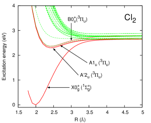
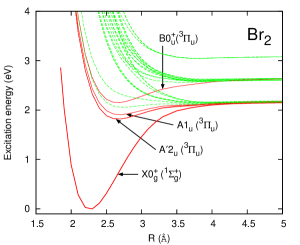
Figure 7: Potential energy curves of Cl₂ (left panel) and Br₂ (right panel).

In order to inspect the effect of atomic weight, or the strength of the spin-orbit couplings, we calculated the molecular factor $C^{a}_{au}$ for the E1$\times$M1 process for Cl₂ and Br₂ molecules with the fixed-nuclei approximation. The arrangements of the potential energy curves of Cl₂ and Br₂ are very similar to that of I₂, as shown in Fig. 7. In both Cl₂ and Br₂, the ground, first and second lowest excited states correspond to the ${X}0_{g}^{+}({}^{1}\Sigma^{+}_{g})$, ${A^{\prime}}2_{u}({}^{3}\Pi_{u})$ and ${A}1_{u}({}^{3}\Pi_{u})$ states, respectively, as in the I₂ case. Also, the location of the $B\ 0_{u}^{+}({}^{3}\Pi_{u})$ state is similar to that of the $B$ state in I₂ molecule. The procedure of the calculation is the same as in the I₂ case described in Sec. 3.1 and 3.2. The molecular factors were evaluated for two different pathways as in the I₂ molecule. In the first case, we took the ${A^{\prime}}2_{u}({}^{3}\Pi_{u})$ state as the initial state and the ${X}0_{g}^{+}({}^{1}\Sigma^{+}_{g})$ as the final state. In the second case, the ${A}1_{u}({}^{3}\Pi_{u})$ state was taken as the initial state and the ${X}0_{g}^{+}({}^{1}\Sigma^{+}_{g})$ was taken as the final state. All other 34 electronic states were considered in the summation of the intermediate state. We selected $R$ = 2.2 and 2.5 Å for Cl₂ and Br₂, respectively, which are the middle points between the equilibrium points of the initial and the final states. In Fig. 8, the molecular factors for I₂, Br₂ and Cl₂ are compared. The molecular factors for the $A\to X$ process are about 10 times larger than those for the $A^{\prime}\to X$ process in all cases of I₂, Br₂ and Cl₂ molecules. The magnitude of the molecular factor is the largest for I₂, the smallest for Cl₂ in both the $A^{\prime}\to X$ and $A\to X$ processes. These differences of magnitudes reflect the differences in strength of the spin-orbit couplings in these three molecules.

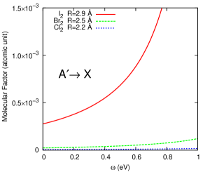
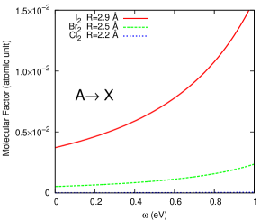
Figure 8: Comparison of the molecular factors $C^{a}_{au}$ in Eq. (8) for I₂, Br₂ and Cl₂ molecules in the fixed-nuclei approximation. The left panel: the $A^{\prime}$ state was used as the $|e\rangle$ state. The right panel: the $A$ state was used as the $|e\rangle$ state. The details of the calculation is the same as in Fig. 3.

We also investigated the lighter molecule, O₂. In this case, the metastable $c{}^{1}\Sigma_{u}^{-}$ state was selected as the initial $|e\rangle$ state, and the $X{}^{3}\Sigma_{g}^{-}$ state as the final $|g\rangle$ state. Using the same procedure as we used for the I₂, Br₂ and Cl₂, the molecular factors for the E1$\times$M1 and M1$\times$E1 are calculated with the fixed-nuclei approximation. The molecular factor of O₂ for the E1$\times$M1 process is approximately $10^{-11}\sim 10^{-10}$ in the energy range $\omega=1\sim 2$ eV, where the $A{}^{3}\Sigma_{u}^{+}$ state has the dominant contribution to the virtual state summation. For the M1$\times$E1 process, the molecular factor is about $10^{-7}$ in the energy range $\omega=1\sim 2$ eV, where the $1{}^{1}\Pi_{g}$ state has the dominant contribution to the virtual state summation. As expected from its small spin-orbit couplings, the molecular factor for O₂ molecule is smaller than the other I₂, Br₂ and Cl₂ molecules: the magnitudes of the molecular factors in the $A\to X$ process are $\sim 10^{-2}$,$\sim 10^{-3}$ and $\sim 10^{-4}$, respectively.

4 RENP spectral rate

A large macroscopic polarization necessary for significant RENP rates is developed by two trigger laser irradiation of frequencies, $\omega$ and $\omega^{\prime}$ with $\omega+\omega^{\prime}=\epsilon_{eg}$. RENP amplitude is proportional to the polarization $\langle g|(R_{1}-iR_{2})/2|p\rangle$ averaged over intermediate states $|p\rangle$. Hence transition to a final single vibrational state $X(v^{\prime})$ for $|g\rangle$ is selected out for the macro-coherently amplified RENP at each experimental setup.

It is appropriate before detailed presentation of numerical results to explain how experimentally neutrino properties and parameters may be determined. Suppose that two continuous wave trigger lasers of frequencies, $\omega+\omega^{\prime}=\epsilon_{eg}$, are irradiated in counter-propagating directions and two exciting pulse lasers of frequencies, $\omega_{P}-\omega_{S}=\epsilon_{eg}$ (in order to induce a Raman-type excitation $|g\rangle\rightarrow|e\rangle$) are suddenly switched on. Only during this pulse irradiation RENP occurs giving a unique signal; asymmetric directional increase of light output of lower frequency $\omega$. If statistics allows, one may hope to measure parity-violating quantities such as emergence of circular polarization from linear polarization. Parity violating quantities that indicate unambiguous signal of involved weak interaction appear with smaller rates, at least by 100, than parity conserving quantities. Observations at different combinations of $(\omega,\omega^{\prime})$ provide spectrum rates at different $\omega$’s, thus covering some range of frequencies that gives the experimentally observed spectrum. After this spectrum determination, one compares the data with theoretical prediction computed assuming some values of undetermined neutrino parameters and properties, and finally the best fit with theoretical calculation determines these parameters.

The experimental method sketched here is by no means unique, and one can think of other schemes. Moreover, many simulations have to be done to determine the signal level once the best method of background rejection is found. It is suggested that the most serious background of the two photon process may be rejected by formation of condensed solitons ptep_overview , which are a target state of coherent macroscopic target entangled by static field condensates.

The quantity $C^{a}(\omega)I(\omega)/C_{0}=C^{a}_{au}(\omega)I(\omega)$ in atomic units is plotted in the following figures except in the last three figures where absolute rates are illustrated for the target parameters of $n=10^{21}$ cm^-3 and $V=10^{2}$ cm³. We used for calculation of the spectral rate numerical values of the mixing angles $\theta_{12},\theta_{13}$, as determined in neutrino oscillation experiments Eq. (2), thus giving numerical weights of six thresholds in Table 2. (As usual, the conventional definition of oscillation angle factors $c_{ij}=\cos\theta_{ij}\,,s_{ij}=\sin\theta_{ij}$ is used in this table.) We also used mass constraints given by oscillation data Eq. (2). The smallest mass defined by $m_{0}$ differs in the NH case where $m_{0}=m_{1}(<m_{2}<m_{3})$ and in the IH case where $m_{0}=m_{3}(<m_{1}<m_{2})$. For large $m_{0}$, NH and IH differences are relatively small: for instance, in the NH case $m_{0}=100$ meV gives three neutrino masses, $m_{1}=100,m_{2}=100.37$, and $m_{3}=111.8$ meV’s, while in the IH case $m_{0}=100$ meV gives $m_{3}=100,m_{1}=111.8$, and $m_{2}=112.1$ meV’s, their mass range within $\sim 10$ %. The mass pattern for a large $m_{0}$ has been called the quasi-degenerate case.

Table 2: The threshold weight $B_{ij}=|a_{ij}|^{2}=|U^{*}_{ei}U_{ej}-\delta_{ij}/2|^{2}$.

$B_{11}$	$B_{22}$	$B_{33}$	$B_{12}+B_{21}$	$B_{23}+B_{32}$	$B_{31}+B_{13}$
$(c_{12}^{2}c_{13}^{2}-1/2)^{2}$	$(s_{12}^{2}c_{13}^{2}-1/2)^{2}$	$(s_{13}^{2}-1/2)^{2}$	$2c_{12}^{2}s_{12}^{2}c_{13}^{4}$	$2s_{12}^{2}c_{13}^{2}s_{13}^{2}$	$2c_{12}^{2}c_{13}^{2}s_{13}^{2}$
0.030	0.039	0.23	0.41	0.015	0.032

In all spectral rate figures we take as the initial state the I₂ $A(v=0)$ state and as the final state various vibrational states of $X(v^{\prime})$. It turns out that numerically dominant contributions are to $X(v^{\prime}=22-26)$. Below we consider $X(v^{\prime}=24)$ as a representative example, since the molecular factors for $X(v^{\prime}=22-26)$ are almost identical. For simplicity we omitted contributions from intermediate states other than the $B$ state, but included all numerically significant vibrational states of $B(v^{\prime\prime})$ as the intermediate state $|p\rangle$. The RENP spectral rate from the metastable $A^{\prime}$ state is calculated in a similar way. The dominant contribution arises from $X(v^{\prime}=20)$. However, the absolute rate is $\sim$ 50 times smaller than in the case of $A(v=0)\rightarrow X(v^{\prime}=24)$.

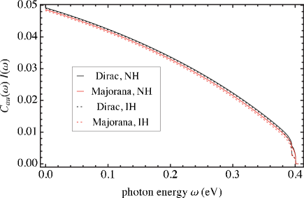
Figure 9: I₂ spectrum $C_{au}(\omega)I(\omega)$ taking $\bar{\epsilon}=\epsilon_{eg}=0.810$ eV for the transition $A(v=0)\rightarrow X(v^{\prime}=24)$. The Dirac NH case in solid black, Majorana NH case of $(\alpha,\beta^{\prime})=(0,0)$ in solid red are compared with the IH cases in dashed colors, taking the smallest neutrino mass of 40 meV.

In Fig. 9 a global photon spectrum in the entire energy region is shown for the transition $A(v=0)\rightarrow X(v^{\prime}=24)$, where four different cases are plotted, NH Dirac in black solid, NH Majorana of $(\alpha,\beta-\delta)=(0,0)$ (the CP conserving case) in red solid, IH Dirac in black dashed, and IH Majorana in red dashed (all with the smallest neutrino mass of 40 meV) comparison_with_i2_ptep . All these cases appear nearly degenerate in the plot.

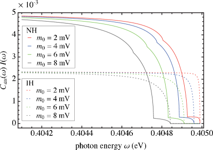
Figure 10: Sensitivity of spectral shape to the smallest neutrino mass values, 2,4,6,8 meV compared for the Majorana case of $(\alpha,\beta^{\prime})=(0,0)$, NH (in solid) and IH (in dashed) cases.

On the other hand, the enlarged spectrum in the threshold region is shown for smaller mass values of $m_{0}$ in Fig. 10. One can clearly observe three kinks in the NH case which are identified as photon energy thresholds of (11), (12), and (22). The other three threshold kinks, (13), (23), and (33), in the NH case are further to the left in this figure. This figure suggests a good chance of determining the smallest neutrino mass at the precision level of 1 meV, if one has a large statistics data in the threshold region.

We shall next examine the possibility of Majorana-Dirac distinction along with determination of CPV phases. The relevant CPV phases $\alpha,\beta,\delta$ in the Majorana case appears in the matrix elements as

$$U_{e1}=\cos\theta_{13}\cos\theta_{12}\,,\hskip 14.22636ptU_{e2}=\cos\theta_{13}\sin\theta_{12}e^{i\alpha}\,,\hskip 14.22636ptU_{e3}=\sin\theta_{13}e^{i(\beta-\delta)}\,.$$ (18)

In the Dirac case there is no CPV phase dependence of the photon energy spectrum rate to this approximation. The parameter $\delta$ alone is accessible independently in neutrino oscillation experiments. These phases appear multiplicatively, in the rate formula around three thresholds of (12), (13) and (23), as

$$\cos 2\alpha\,,\hskip 14.22636pt\cos 2(\beta-\delta)\,,\hskip 14.22636pt\cos 2(\alpha-\beta+\delta)\,,$$ (19)

which are further multiplied by the weight factor of Table 2 ptep_overview times a product of two masses $m_{i}m_{j},i\neq j$. There is thus no doubt that the Majorana-Dirac distinction is easier for larger neutrino masses. We shall introduce a new notation of CPV phase $\beta^{\prime}\equiv\beta-\delta$ to simplify the formulas. The case $(\alpha,\beta^{\prime})=(0,0)$ corresponds to CP conserving (CPC) Majorana neutrino pair emission.

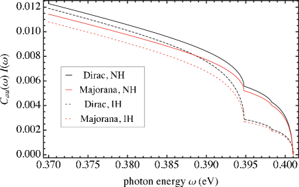
Figure 11: CP conserving Majorana case of $(\alpha,\beta^{\prime})=(0,0)$ vs Dirac distinction, Dirac in black, Majorana in red. The smallest neutrino mass of 40 meV, and NH (in solid) and IH (in dashed) cases are assumed.

As is evident in Fig. 11, the Majorana-Dirac distinction in the proposed de-excitation of I₂ appears easier than NH-IH distinction at low enough photon energies where rates are largest. Numerically, the I₂ CPC Majorana rate for $m_{0}=40$ meV is significantly different from the Dirac rate by $\sim 0.07$ at a photon energy 0.37 eV, while this difference for Xe $J=2$ transition ptep_overview never exceeds 0.2 % at all photon energies.

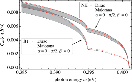
Figure 12: Majorana $\alpha$-band and Dirac photon spectrum for $A(v=0)\rightarrow X(v^{\prime}=24)$. Majorana band defined by variation of $\alpha$ in the range $0\sim\pi/2$ with a fixed $\beta^{\prime}=0$. Dirac NH is given in solid red and Dirac IH in dashed red, while the upper(lower) band corresponds to NH(IH). The smallest neutrino mass of 40 meV is assumed.

Study of the sensitivity to the CPV phase $\alpha,\beta^{\prime}$ however requires a more careful analysis, because the CPC case of $(\alpha,\beta^{\prime})=(0,0)$ gives the largest destructive interference due to the effect of identical Majorana fermions, hence the Majorana-Dirac distinction is easiest in this case. It is thus necessary to vary the CPV phases $(\alpha,\beta^{\prime})$ in their allowed range. It turns out that with the given numerical weight factors of Table 2 dependence of spectral rates on $\beta^{\prime}$ is much weaker than on $\alpha$. The most prominent kinks are at the (12) and (33) thresholds and the highest sensitivity to $\alpha$ arises from the (12) threshold. Under this circumstance we may introduce a useful concept of Majorana $\alpha-$band which is defined by the region of spectral rates, bounded by the largest Majorana rate at $\alpha=\pi/2$ and the smallest rate at $\alpha=0$. We illustrate this band structure in Fig. 12. Strictly, the $\alpha-$band is defined for $\beta^{\prime}=0$, but dependence of the band shape on $\beta^{\prime}$ is small and we may approximately use the $\alpha-$band terminology for any value of $\beta^{\prime}$.

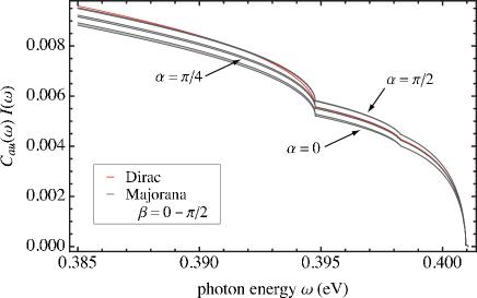
Figure 13: Majorana $\beta$-bands (shaded region bounded by black curves) for 3 values of $\alpha=0,\pi/4,\pi/2$ which are well separated and Dirac (in red) photon spectrum for $A(v=0)\rightarrow X(v^{\prime}=24)$. A Majorana $\beta$-band is defined by variation of $\beta$ in the range $0\sim\pi/2$ with a fixed $\alpha$. NH case is shown. The smallest neutrino mass of 40 meV is assumed.

On the other hand, variation of $\beta^{\prime}$ gives much smaller band widths, and moreover these bands are separated as $\alpha$ values vary, as shown in Fig. 13. It implies that experimental determination of $\beta^{\prime}$ is much more difficult than $\alpha$ in the proposed I₂ de-excitation scheme. We shall concentrate on determination of the CPV parameter $\alpha$ in the following.

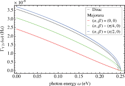
Figure 14: Three Majorana cases and Dirac case of the photon spectrum for $A(v=0)\rightarrow X(v^{\prime}=24)$. NH in solid and IH in dashed. Different colors correspond to Dirac and a few Majorana cases; Dirac in black, Majorana of $(\alpha,\beta)=(0,0)$ in red, Majorana of $(\alpha,\beta)=(\pi/2,0)$ in blue, and Majorana of $(\alpha,\beta)=(\pi/4,0)$ in green. The smallest neutrino mass of 250 meV is assumed. The transition $A(v=0)\rightarrow X(v^{\prime}=25)$ gives similar, but slightly smaller rate curves.

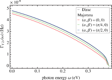
Figure 15: Similar plot to Fig. 14 for $m_{0}=100$ meV and $A(v=0)\rightarrow X(v^{\prime}=24)$.

The spectral rate for a large value of the smallest neutrino mass, 250 meV (a quasi-degenerate mass not excluded by the cosmological bound cosmological_bound ) is shown in Fig. 14, which shows a great sensitivity to the Majorana-Dirac distinction for this quasi-degenerate case. Another example of spectral rate is shown for $m_{0}=100$ meV in Fig. 15 where the Dirac case and the Majorana case of $\alpha=\pi/2$ become nearly degenerate in the plot. Thus, for relatively smaller mass values of $m_{0}$ one needs more detailed study, both by theoretical means and numerical simulations, for determination of the $\alpha$ parameter, which is beyond the scope of the present work.

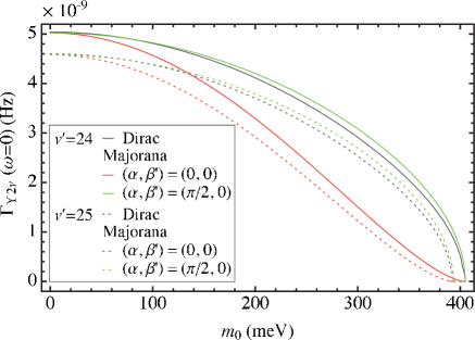
Figure 16: Zero energy limits of NH absolute spectrum rates (in the unit of $10^{-11}$ Hz) are shown for two transitions to $X(v^{\prime}=24)$ (in solid) and $X(v^{\prime}=25)$ (in dashed). The Dirac cases are given in black, while the Majorana cases of $(\alpha,\beta)=(0,0)$ are given in red and the $(\pi/2,0)$ cases are in green. The target parameters are $n=10^{21}\ \text{cm}^{-3}$ and $V=10^{2}\$cm³. $\epsilon_{eg}=0.787$ eV was used for $X(v^{\prime}=25)$.

It is important to note that comparison of two de-excitation to $X(v^{\prime}=24$ and 25) offers a good tool of unambiguous experimental identification of RENP (this can be done by a change of one of two trigger lasers). This is an advantage of molecular targets, since one may compare two spectra of different transitions without much relying on the absolute rate scale. The zero photon energy limit of absolute spectrum gives an overall magnitude of the RENP rate, which then indicates relative difference of these two different transitions. We plot in Fig. 16 these values for transitions to $X(v^{\prime}=24$ and 25) as functions of the smallest neutrino mass $m_{0}$, which shows insensitivity of rates for $m_{0}<O(30)$ meV. There is an interesting phenomenon of crossover of rates occurring at two points of the smallest mass $m_{0}\sim 140$ meV and $\sim 390$ meV. For the range of $\alpha$ parameter between these two values Dirac and Majorana $(\pi/2,0)$ rates to $X(v^{\prime}=25)$ of smaller atomic energy separation overtake Majorana $(0,0)$ rate to $X(v^{\prime}=24)$ of larger separation. The simultaneous use of different vibrational transitions of molecules may be effective for RENP identification and exploration of the neutrino mass range as well.

The actual rate at each photon energy is equal to the plotted values $C_{au}(\omega)I(\omega)$ multiplied by the factor

$$\Gamma_{dm}C_{0}\sim 1.0\times 10^{-7}\ \text{Hz}\left(\frac{n}{10^{21}\ \text{cm}^{-3}}\right)^{3}\frac{V}{10^{2}\ \text{cm}^{3}}\left(\frac{\epsilon_{eg}}{0.810\ \text{eV}}\right)^{3}\,.$$ (20)

Note that we took $\eta_{\omega}(t)=1$ which is however expected to be smaller than 1.

Let us compare I₂ RENP rate with Xe rate. The I₂ rate is calculated as $\sim 5$ nHz at $\omega=0$, assuming targets with $n=10^{21}$ cm^-3, $V=10^{2}$ cm³, and $\eta_{\omega}=1$. Under the same experimental condition of targets, the overall RENP rate for Xe atom is much larger, by $\sim 10^{5}$. The origin of this large rate difference is explained as follows. Dependence of the RENP rate (for definiteness at $\omega=0$) is roughly given by product of factors as

$$\Gamma_{\gamma 2\nu}(0)\propto G_{F}^{2}n^{3}Vd^{2}S^{2}\frac{\epsilon_{eg}^{3}}{\epsilon_{pg}^{2}}\,,$$ (21)

where we used $d$ and $S$ to mean the magnitudes of dipole and the spin factor in the RENP amplitude. Relation $\epsilon_{eg}\approx\epsilon_{pg}$ approximately holds both for Xe and I₂. An extra $n$-dependence in addition to the basic macro-coherence dependence $\propto n^{2}$ arises by our assumption of taking the maximal RENP rate ($\eta_{\omega}=1)$, with the stored field energy density of $|\vec{E}|^{2}=\epsilon_{eg}n$. Difference of $\epsilon_{eg}$ between Xe and I₂ is $\sim 10$ and the spin factor is of the same order of unity for two targets. The Franck-Condon like suppression factor fc_factor intrinsic to molecules is only 0.03 for I₂. The rest of rate difference by $\sim 300$ is attributed to difference in the transition dipole moment of Xe and I₂. Unlike the simple dipole transition $6s\rightarrow 5p$ in Xe atom the I₂ molecular dipole arises from $B(^{3}\Pi_{u})\rightarrow X(^{1}\Sigma_{g}^{+})$ involving different configurations and is much suppressed. We definitely need solid environment of the target number density of $O(10^{23})$ cm^-3 for realistic I₂ RENP experiments, which is a challenge left to experimentalists. A molecule closer to Xe with respect RENP appears to be CsI.

5 Summary

An attractive feature of using molecules is that there are many vibrational states available as a final molecular state for RENP which makes easier experimental identification of the process. We computed the RENP spectrum rate for homo-nuclear diatomic molecules of isovalent series, Cl₂, Br₂ and I₂ and found that the rate becomes larger as the atomic number increases, as is expected. Even the largest I₂ rate is, however, much smaller than Xe atom rate. The distinction of Dirac-Majorana neutrinos and the determination of some range of the new CPV phase $\alpha$ are possible at photon energies where rates are largest for the quasi-degenerate neutrino masses. The NH-IH distinction along with the smallest mass measurement can be done around the threshold region.

Appendix A Appendix: Comparison of the contributions from the $A$ and $B^{\prime\prime}$ states in the I₂ $A^{\prime}\to X$ process, including the effect of nuclear motion

In the left panel of Fig. 3, with the fixed-nuclei approximation, the contribution of the $B^{\prime\prime}$ state to the molecular factor in the $A^{\prime}\to X$ process looks close to that of the $A$ state at low energy region. Although we calculated the molecular factor for the $A^{\prime}\to X$ process considering only the $A$ intermediate state in section 3.3, it is not clear if the $A$ state has really larger contribution for the molecular factor $C^{a}_{au}$ for the E1$\times$M1 process than the $B^{\prime\prime}$ state has, when the effect of nuclear motion is considered. Here, we evaluate the amplitude of the first term in the bracket of Eq. (4), including nuclear motion, separately for the $A$ and $B^{\prime\prime}$ states, and estimate their contributions to the molecular factor. The reason for not treating molecular factor $C^{a}_{au}$ directly, but evaluating the first term in the bracket of Eq. (4) is that the $B^{\prime\prime}$ state is repulsive, see Fig. 2, and it is difficult to treat continuum nuclear wavefunctions in the expression of Eq. (8). The first term in the bracket of Eq. (4), on the other hand, can be easily evaluated using the following expression:

$$\sum_{p}\frac{\langle g|d|p\rangle\langle p|S|e\rangle}{E_{p}-E_{g}-\omega}=\lim_{\epsilon\to+0}i\int_{0}^{\infty}dte^{it\left(\omega+E_{g}\right)}\langle g|de^{-it\left(\hat{H}-i\epsilon\right)}S|e\rangle$$ (22)

where $\hat{H}|p\rangle=E_{p}|p\rangle$ is assumed. This equation represents the Green’s function by integral in time domain LevineBook , and can be evaluated by the Fourier transform of the correlation function $\langle g|de^{-it\left(\hat{H}-i\epsilon\right)}S|e\rangle$ obtained by solving time-dependent Schrödinger equation. For our purpose, the vibrational (nuclear) Hamiltonian on the $A$ or $B^{\prime\prime}$ electronic state is used for $\hat{H}$.

As a test, we evaluated the right hand side and the left hand side of Eq. (22) separately for the I₂ $A^{\prime}\to A\to X$ process using explicit summation of the vibrational states, and the wavepacket propagation on the $A$ state, respectively. The same DVR basis parameters were used as in Sec. 3.3. The wave packet was propagated by expanding the time evolution operator in terms of Chebyshev polynomials ISI:A1984TS41400029 , with $\Delta t$ = 0.1 fs. Since many bound vibrational eigenstates contribute to the time evolution of the wavepacket, we need relatively long total propagation time, 7.0 ps. In addition, we had to leave small but finite value of $\epsilon$, $10^{-4}$ a.u., in order to converge the Fourier transform in the right hand side of Eq. (22). As shown in Fig. 17, numerical values of the left hand side and right hand side of Eq. (22) agree perfectly well in case of the $A$ electronic state.

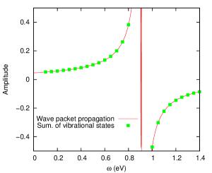
Figure 17: Comparison of Eq. (22) evaluated by the vibrational state summation ($v=0-19$) and the wave packet propagation on the I₂ $A1_{u}$ intermediate electronic state, using the I₂ $A^{\prime}(v=0)$ state as the initial state, and the $X(v^{\prime}=20)$ state as the final state.

For the wavepacket calculation on the $B^{\prime\prime}$ state, the same DVR basis parameters were used. Since the $B^{\prime\prime}$ state is repulsive, we need to put the absorbing potential from $R$ = 5.0 to 7.0 Å to prevent artificial reflection of the wavepacket at the boundary. This absorbing potential can be regarded as decay of the wavepacket into $R=\infty$. The wave packet on the $B^{\prime\prime}$ potential energy curve with the specific initial state $S|A^{\prime}(v)\rangle$, where $A^{\prime}(v)$ represents the vibrational state on the $A^{\prime}$ state, is propagated by expanding the time evolution operator in terms of Chebyshev polynomials ISI:A1984TS41400029 , with $\Delta t$ = 0.1 fs. The total propagation time is 400 fs, which is much shorter than the time needed in the wave packet propagation on the $A$ electronic state. This short propagation time can be attributed to the fact that the wave packet is not reflected, but just absorbed in 400 fs at the right-hand side of the $B^{\prime\prime}$ potential energy curve. The diploe and spin transition moments, necessary to evaluate Eq. (22) are shown in Fig. 18.

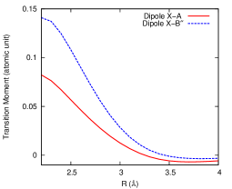
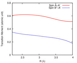
Figure 18: Left panel: Electric dipole transition moment between the $X$ and $A$ states of I₂ (red solid line), and between the $X$ and $B^{\prime\prime}$ states (blue dashed line). Right panel: Spin transition moment between the $A$ and $A^{\prime}$ states (red solid line), and between the $B^{\prime\prime}$ and $A^{\prime}$ states (blue dashed line).

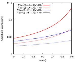
Figure 19: Comparison of the amplitudes, Eq. (22), with the $A1_{u}$ and $B^{\prime\prime}1_{u}$ intermediate electronic states, obtained by the wavepacket calculations. The initial states are $A^{\prime}(v=0)$, and the final states are $X(v^{\prime}=16,20)$.

The amplitudes for the $A^{\prime}\to X$ process with the $A$ and $B^{\prime\prime}$ intermediate electronic states, obtained by the wavepacket calculations, are compared in Fig. 19. When the initial vibrational state is $A^{\prime}(v=0)$ and the final vibrational state is $X(v^{\prime}=20)$, the amplitude of the $A$ state at $\omega=0.4$ eV is about 60 % larger than that of the $B^{\prime\prime}$ state. This means that the molecular factor including the $A$ intermediate state is approximately 2.5 times larger than that including the $B^{\prime\prime}$ intermediate state. Although the contribution of the $B^{\prime\prime}$ state is not negligible, for the purpose of the present study, the molecular factor may be safely approximated by including only the $A$ electronic state.

References

- (1) G. L. Fogli, E. Lisi, A. Marrone, D. Montanino, A. Palazzo, and A. M. Rotunno, Phys. Rev. D 86, 013012 (2012); Other fits of references, M.C. Gonzalez-Garcia, Michele Maltoni, Jordi Salvado, and Thomas Schwetz, J. High Energ. Phys. 2012, 1–24 (2012) and D. V. Forero, M. Tórtola, and J. W. F. Valle, Phys. Rev. D 86, 073012 (Oct 2012) give almost identical values of mass squared differences and , , but different numbers for , which is not used for our RENP rate calculation.
- (2) Cosmological bounds are summarized in J. Beringer et al., Phys. Rev. D 86, 010001 (Jul 2012). They quote the bound (0.31.3) eV at 95 % confidence level.
- (3) The massive Majorana neutrino is described by a relativistically covariant two-component spinor and satisfies the Majorana equation (unlike the Dirac equation for four-component spinors). The particle number is ill-defined in the Majorana equation, and violates the U(1) symmetry associated with the lepton number. The quasi-particle of Majorana nature discussed in condensed matter physics is different in its dispersion relation from the massive Majorana neutrino in particle physics.
- (4) A. Fukumi, S. Kuma, Y. Miyamoto, K. Nakajima, I. Nakano, H. Nanjo, C. Ohae, N. Sasao, M. Tanaka, T. Taniguchi, S. Uetake, T. Wakabayashi, T. Yamaguchi, A. Yoshimi, and M. Yoshimura, Prog. Theor. Exp. Phys. 2012(1) (2012), arXiv:1211.4904v1 [hep-ph] and references cited therein.
- (5) The weak interaction Hamiltonian is adequately described here by the four-Fermi contact interaction. For relation to the W- and Z-exchange fundamental interaction in the standard electroweak theory, see any standard textbook such as E. D. Commins and P. H. Bucksbaum, Weak interactions of leptons and quarks, (Cambridge University Press, New York, 1983).
- (6) M. Yoshimura, N. Sasao, and M. Tanaka, Phys. Rev. A 86, 013812 (2012), arXiv:1203.5394 [quan-ph].
- (7) M. Yoshimura, Phys. Lett. B 699, 123 (2011) and references therein.
- (8) D. N. Dinh, S. Petcov, N. Sasao, M. Tanaka, and M. Yoshimura, Phys. Lett. B 719, 154 – 163 (2012), arXiv:1209.4808v1 [hep-ph].
- (9) M. Fukugita and T. Yanagida, Phys. Lett. B 174(1), 45 – 47 (1986).
- (10) S. Davidson and A. Ibarra, Nucl. Phys. B 648(12), 345 – 375 (2003) and references therein.
- (11) R. S. Mulliken, J. Chem. Phys. 55(1), 288–309 (1971).
- (12) C. Teichteil and M. Pelissier, Chem. Phys. 180(1), 1–18 (1994).
- (13) W. A. de Jong, L Visscher, and W. C. Nieuwpoort, J. Chem. Phys. 107(21), 9046–9058 (1997).
- (14) For instance, G. Herzberg, Molecular Spectra and Molecular Structure: I. Spectra of Diatomic Molecules, (Krieger Publishing, Malabar, second edition, 1989).
- (15) H.-J. Werner, Mol. Phys. 89, 645–661 (1996).
- (16) P. Celani and H.-J. Werner, J. Chem. Phys. 112, 5546–5557 (2000).
- (17) P. J. Knowles and H.-J. Werner, Chem. Phys. Lett. 115(3), 259–267 (1985).
- (18) H.-J. Werner and P. J. Knowles, J. Chem. Phys. 82(11), 5053–5063 (1985).
- (19) B. O. Roos, R Lindh, P. A. Malmqvist, V Veryazov, and P. O. Widmark, J. Phys. Chem. A 108, 2851–2858 (2004).
- (20) M. Reiher and A. Wolf, J. Chem. Phys. 121, 2037–2047 (2004).
- (21) M. Reiher and A. Wolf, J. Chem. Phys. 121, 10945–10956 (2004).
- (22) A. Wolf, M. Reiher, and B. A. Hess, J. Chem. Phys. 117, 9215–9226 (2002).
- (23) A. Berning, M Schweizer, H.-J. Werner, P. J. Knowles, and P Palmieri, Mol. Phys. 98, 1823–1833 (2000).
- (24) P. A. Malmqvist, B. O. Roos, and B Schimmelpfennig, Chem. Phys. Lett. 357, 230–240 (2002).
- (25) H.-J. Werner, P. J. Knowles, F. R. Manby, M. Schütz, P. Celani, G. Knizia, T. Korona, R. Lindh, A. Mitrushenkov, G. Rauhut, T. B. Adler, R. D. Amos, A. Bernhardsson, A. Berning, D. L. Cooper, M. J. O. Deegan, A. J. Dobbyn, F. Eckert, E. Goll, C. Hampel, A. Hesselmann, G. Hetzer, T. Hrenar, G. Jansen, C. Köppl, Y. Liu, A. W. Lloyd, R. A. Mata, A. J. May, S. J. McNicholas, W. Meyer, M. E. Mura, A. Nicklass, P. Palmieri, K. Pflüger, R. Pitzer, M. Reiher, T. Shiozaki, H. Stoll, A. J. Stone, R. Tarroni, T. Thorsteinsson, M. Wang, and A. Wolf, Molpro, version 2010.1, a package of ab initio programs (2010).
- (26) T. Ishiwata, H. Ohtoshi, M. Sakaki, and I. Tanaka, J. Chem. Phys. 80(4), 1411–1416 (1984).
- (27) J. Tellinghuisen, J. Chem. Phys. 58(7), 2821–2834 (1973).
- (28) J. B. Koffend, A. M. Sibai, and R. Bacis, J. Phys. France 43(11), 1639–1651 (1982).
- (29) S. Gerstenkorn, P. Luc, and J. Verges, J. Phys. B 14(5), L193–L196 (1981).
- (30) J. Tellinghuisen, J. Chem. Phys. 82(9), 4012–4016 (1985).
- (31) J. Tellinghuisen, J. Chem. Phys. 76(10), 4736–4744 (1982).
- (32) F. Martin, R. Bacis, S. Churassy, and .J Verges, J. Mol. Spectrosc. 116(1), 71–100 (1986).
- (33) A. J. C. Varandas, Adv. Chem. Phys. 74, 255–338 (1988).
- (34) D. T. Colbert and W. H. Miller, J. Chem. Phys. 96(3), 1982–1991 (1992).
- (35) Due to a non-trivial dependence of the molecular factor as calculated in the preceding section, the overall spectral form shown in Fig. 9 is considerably different from the one previously given in Ref. ptep_overview where the precise calculation of is not attempted and the dependence of has been ignored.
- (36) In Ref. ptep_overview the Franck-Condon factor of I2 was calculated using the Morse potential where relevant parameters are determined by experimental data. Our new rate estimate for the transition gives a value arising from the Franck-Condon factor.
- (37) R. D. Levine, Quantum mechanics of molecular rate processes, page 19, Oxford (1969).
- (38) H. Tal-Ezer and R. Kosloff, J. Chem. Phys. 81, 3967–3971 (1984).