HD 285507b: An Eccentric Hot Jupiter in the Hyades Open Cluster

Abstract

We report the discovery of the first hot Jupiter in the Hyades open cluster. HD 285507b orbits a $V=10.47$ K4.5V dwarf ($M_{*}=0.734~{}{M_{\odot}}$; $R_{*}=0.656~{}{R_{\odot}}$) in a slightly eccentric ($e=0.086^{+0.018}_{-0.019}$) orbit with a period of $6.0881^{+0.0019}_{-0.0018}$ days. The induced stellar radial velocity corresponds to a minimum companion mass of $M_{\rm P}\sin{i}=0.917\pm 0.033~{}{M_{\rm Jup}}$. Line bisector spans and stellar activity measures show no correlation with orbital phase, and the radial velocity amplitude is independent of wavelength, supporting the conclusion that the variations are caused by a planetary companion. Follow-up photometry indicates with high confidence that the planet does not transit. HD 285507b joins a small but growing list of planets in open clusters, and its existence lends support to a planet formation scenario in which a high stellar space density does not inhibit giant planet formation and migration. We calculate the circularization timescale for HD 285507b to be larger than the age of the Hyades, which may indicate that this planet’s non-zero eccentricity is the result of migration via interactions with a third body. We also demonstrate a significant difference between the eccentricity distributions of hot Jupiters that have had time to tidally circularize and those that have not, which we interpret as evidence against Type II migration in the final stages of hot Jupiter formation. Finally, the dependence of the circularization timescale on the planetary tidal quality factor, $Q_{\rm P}$, allows us to constrain the average value for hot Jupiters to be $\log{Q_{\rm P}}=6.14^{+0.41}_{-0.25}$.

1. Introduction

The efforts of more than two decades of exoplanet searches have produced an incredible diversity of discoveries, many of which bear little similarity to planets in the solar system. These discoveries provide valuable constraints for our theories of planet formation, which have evolved to explain the existence of the wide array of planetary systems observed. One such grouping of planets is the hot Jupiters, gas giant planets in short period orbits (defined herein as $M_{\rm P}>0.3~{}{M_{\rm Jup}}$ and $P<10$ days), which occur at rates of $\mathord{\sim}1.2\%$ around Sun-like field stars (see Wright et al., 2012; Mayor et al., 2011). However, more than $60$ years after their proposed existence (Struve, 1952) and nearly $20$ years after the first detection (Mayor & Queloz, 1995), we still lack a complete description of the hot Jupiter formation process. It is believed that they form beyond the snow line (located at $\mathord{\sim}2.7$ AU for the current-day Sun; e.g., Martin & Livio, 2013) where there is a greater reservoir of solids with which to build a massive core (e.g., Kennedy & Kenyon, 2008) before undergoing an inward migration process, but many questions remain to be answered.

While there are many mechanisms that could cause a gas giant planet to lose angular momentum and migrate inward (see a discussion in Ford & Rasio, 2008), two leading ideas are dynamical interactions with a circumstellar disk (“Type II” migration; Goldreich & Tremaine, 1980; Lin & Papaloizou, 1986) and multi-body gravitational interactions with other planetary (“planet-planet scattering”; e.g., Rasio & Ford, 1996; Juric & Tremaine, 2008) or stellar (Kozai cycles; e.g., Fabrycky & Tremaine, 2007) companions. Migration through a disk must occur while the gas disk is present (within $\mathord{\sim}10$ Myr; Haisch et al., 2001) and is expected to preserve near-circular orbits, but if multi-body interactions are the source of most hot Jupiters, inward migration may take significantly longer and many of these planets should initially possess high eccentricity. For simplicity, we adopt the language of Socrates et al. (2012) and refer to these multi-body processes as “high eccentricity migration” (HEM). Given the different timescales predicted, one direct way to distinguish between mechanisms would be to search for hot Jupiters orbiting very young stars ($\lesssim 10$ Myr), and at least one promising candidate exists orbiting a T-Tauri star (PTFO 8-8695; van Eyken et al., 2012; Barnes et al., 2013). However, the enhanced activity associated with young stars presents significant challenges for such surveys (e.g., Bailey et al., 2012). Alternatively, the dynamical imprint of HEM on the orbital eccentricity could provide a more accessible means to observationally constrain migration (e.g., Dawson & Murray-Clay, 2013; Dong et al., 2014). Subsequent tidal circularization of the orbits erases this evidence of multi-body interaction over time, so identifying “dynamically young” systems, for which the system age ($t_{\rm age}$) is less than the circularization timescale ($\tau_{\rm cir}$), is necessary for such an investigation. Longer period planets (large $\tau_{\rm cir}$) could satisfy this requirement, but hot Jupiters with periods of only a few days are both more common and easier to detect. Young planets (small $t_{\rm age}$) offer another solution, but field stars tend to be old and their ages are difficult to estimate accurately (Mamajek & Hillenbrand, 2008). The ages of open clusters, on the other hand — e.g., the $625$ Myr Hyades (Perryman et al., 1998) or the $125$ Myr Pleiades (Stauffer et al., 1998) — are typically precisely known and can be comparable to (or less than) the circularization timescales of many hot Jupiters. Consequently, planets in clusters could provide an avenue to directly measure this observational signature of HEM, allowing us to determine which process is most important for hot Jupiter migration.

With the recent discovery of two hot Jupiters (Quinn et al., 2012) in the Praesepe open cluster ($\mathord{\sim}600$ Myr), it is now clear that giant planets can form and migrate in a dense cluster environment. This had been an open question, as previous exoplanet surveys targeting open clusters — including high resolution spectroscopy of $94$ dwarfs in the Hyades (Paulson et al., 2004, hereafter P04) and $58$ dwarfs in M67 (Pasquini et al., 2012), as well as transit photometry of several other clusters (e.g., Hartman et al., 2009; Pepper et al., 2008; Mochejska et al., 2006) — had not discovered any planets. However, while small planets do appear to be a common by-product of star formation, giant planets are comparatively rare (e.g., Fressin et al., 2013). Most cluster surveys have not been sensitive to the more common smaller planets, so it is likely that small sample sizes are to blame for the null results (see also van Saders & Gaudi, 2011). Indeed, two mini-Neptunes recently discovered (Meibom et al., 2013) in NGC 6811 ($\mathord{\sim}1$ Gyr, Meibom et al., 2011) by the Kepler spacecraft would not have been detected by previous surveys, and the results suggest consistency between occurrence rates in open clusters and the field for planets of all sizes.

While open cluster planet surveys have recently enjoyed successes in measuring planet formation rates, they have not yet provided a convincing constraint for the hot Jupiter migration process, despite their potential to do so in the long term. Unfortunately, the hot Jupiters discovered in Praesepe are too old to address timescale differences between migration mechanisms, and they are not dynamically young, either. That is, they are close enough to their stars to have already undergone tidal circularization ($t_{\rm age}>\tau_{\rm cir}$). To see the dynamical imprint of migration it will thus be necessary to identify younger hot Jupiters or hot Jupiters on wider orbits that would still bear the signature of dynamical scattering in order to help distinguish between migration mechanisms. In hopes of accomplishing the latter, here we extend our radial velocity (RV) survey to include more stars with ages and properties comparable to those in Praesepe.

We describe our sample selection in Section 2 and outline our spectroscopic and photometric observations and analysis in Sections 3 and 4. We then present evidence for high eccentricity migration and a constraint on $Q_{\rm P}$ in Sections 5$-$7, and in Section 8 we discuss our results.

2. Sample Selection

Hyades cluster members represent an ideal sample for extending our survey of Sun-like stars in Praesepe (Quinn et al., 2012). The two clusters are nearly the same age ($625$ Myr and $578$ Myr, respectively; Perryman et al., 1998; Delorme et al., 2011), and both are metal-rich — ${\rm[Fe/H]}=+0.13\pm 0.01$ (Hyades, Paulson et al., 2003) and $+0.19\pm 0.04$ (Praesepe, Quinn et al., 2012). While P04 found no planets among $94$ Hyades dwarfs ($74$ FGK stars), a primary motivation of their survey was to explore the relationship between planet occurrence and stellar mass, so a number of FGK stars were omitted in favor of including $20$ M stars. As a result, some suitable stars have not yet been observed with precise radial velocities.

Our potential targets come from a list assembled by Robert Stefanik for the CfA Hyades binary survey (R. Stefanik 2013, private communication). Since $1979$, the CfA has been monitoring over $600$ stars in the Hyades field, extending to a magnitude of $V=15$. Originally the program consisted of stars drawn from the Hyades lists of van Bueren (1952), van Altena (1966), and Pels et al. (1975). Over the years additional stars were added to the observing program if there was some suggestion that the stars were possible members based on photometric, proper motion, or radial velocity investigations of the cluster. Also added to the CfA program were the companion stars of Hyades visual binaries. From this parent list, the sample surveyed here was determined after excluding close ($<1\farcs 0$) visual binaries revealed by high-resolution imaging (Patience et al., 1998), the $94$ stars previously surveyed by P04, rapid rotators ($v\sin(i)>30~{}{\rm km\thinspace s^{-1}}$), faint targets ($V>12$), and spectroscopic binaries (with orbits or long-term trends) from the literature and the CfA survey. The final target list contained $27$ FGK Hyades members (see Table 1).

Table 1Target List and Observations Summary

Star	Other Name	$\alpha$	$\delta$	$V$	$N$	$\sigma_{\rm obs}$	$v\sin{i}$
		(J2000)	(J2000)	(mag)		(m s-1)	(km s-1)
J202A	HIP 15300	$03:17:22.6$	$+26:18:55$	$11.10$	$6$	$39.8$	$2.2$
H24098C	HD 24098C	$03:50:13.1$	$-01:31:08$	$11.20$	$9$	$40.3$	$0.9$
L7	HD 283044	$03:52:40.8$	$+25:48:16$	$11.10$	$5$	$12.9$	$2.0$
G7-73C	$\cdots$	$04:01:12.8$	$+12:05:48$	$11.30$	$7$	$40.0$	$2.9$
L15	HD 285507	$04:07:01.0$	$+15:20:07$	$10.47$	$32$	$89.5$	$3.2$
L18	HD 284155	$04:08:36.0$	$+23:46:07$	$9.42$	$7$	$25.8$	$2.0$
VB13	HD 26345	$04:10:42.3$	$+18:25:24$	$6.59$	$5$	$78.8$	$28.7$
VB14	HD 26462	$04:11:20.2$	$+05:31:23$	$5.70$	$24$	$608.4$	$17.6$
H111	HD 286589	$04:14:51.7$	$+13:03:18$	$10.68$	$6$	$22.5$	$2.1$
L26	HD 285630	$04:17:25.0$	$+19:01:47$	$10.80$	$5$	$23.7$	$2.3$
H210	HD 286693	$04:19:36.9$	$+12:37:27$	$9.80$	$6$	$7.5$	$0.6$
H246	HD 27561	$04:21:34.7$	$+14:24:35$	$6.58$	$5$	$30.6$	$22.1$
L38	$\cdots$	$04:24:07.2$	$+22:07:08$	$10.95$	$5$	$8.5$	$3.0$
H342	HD 285742	$04:25:00.1$	$+16:59:05$	$10.37$	$8$	$14.4$	$1.5$
L58	HD 284455	$04:26:47.3$	$+21:14:05$	$11.24$	$10$	$21.8$	$2.6$
G7-227	HD 285765	$04:27:56.7$	$+19:03:39$	$11.36$	$6$	$17.9$	$1.7$
H422	HD 285804	$04:28:10.6$	$+16:28:14$	$10.72$	$5$	$23.3$	$2.5$
H469	HD 28406	$04:29:30.0$	$+17:51:48$	$6.89$	$5$	$54.3$	$33.4$
H472	HD 285805	$04:29:30.9$	$+16:14:42$	$10.63$	$8$	$19.0$	$1.9$
VB86	HD 28608	$04:30:56.7$	$+10:45:07$	$7.03$	$5$	$55.1$	$30.0$
G8-64	HD 284785	$04:47:08.5$	$+20:52:58$	$9.77$	$6$	$28.8$	$4.3$
AK2-1315	$\cdots$	$04:47:18.0$	$+06:27:12$	$11.35$	$7$	$7.0$	$2.0$
VB116	HD 30505	$04:49:03.0$	$+18:38:30$	$8.97$	$8$	$28.6$	$4.0$
L96	HD 286085	$04:50:00.4$	$+16:24:45$	$10.73$	$7$	$28.8$	$3.6$
+23755	HD 284855	$04:53:00.6$	$+23:29:18$	$10.61$	$7$	$15.2$	$1.7$
L101	BD +13 741	$04:57:00.4$	$+13:54:46$	$10.86$	$7$	$45.0$	$3.9$
VB128	HD 31845	$04:59:44.0$	$+15:55:03$	$6.75$	$5$	$47.9$	$34.9$

3. High Resolution Spectroscopy

3.1. Spectroscopic Observations

The Tillinghast Reflector Echelle Spectrograph (TRES; Fűrész, 2008) mounted on the $1.5$ m Tillinghast Reflector at the Fred L. Whipple Observatory (FLWO) on Mt. Hopkins, AZ was used to obtain high resolution spectra of Hyades members between UT 2012 September 23 and 2013 April 08. TRES is a temperature-controlled, fiber-fed instrument with a resolving power of $R\mathord{\sim}44,000$ and a wavelength coverage of $\mathord{\sim}3850$–$9100$ Å, spanning $51$ echelle orders.

In order to achieve a sensitivity to planets similar to that achieved for Praesepe stars, we strove to observe each star on two to three consecutive nights, followed by another two to three consecutive nights $\mathord{\sim}1$ week later (see Quinn et al., 2012). This strategy, given the RV precision of TRES, is sensitive to planets with masses greater than about $0.5~{}{M_{\rm Jup}}$ and periods up to $10$ days. Though we were sometimes forced to deviate from the planned observing cadence because of weather and instrument availability, we were able to obtain at least $5$ spectra of each of our $27$ stars. Exposure times ranged from $1$–$25$ minutes, yielding a typical S/N per resolution element of at least $40$. We also obtained nightly observations of the nearby IAU RV standard stars HD 38230 ($28^{\circ}$ away) and HD 3765 ($54^{\circ}$ away) to help track instrument stability and correct for any RV zero point drift. Precise wavelength calibration was established by obtaining ThAr emission-line spectra before and after each spectrum, through the same fiber as the science exposures.

Compared to the sample in P04, we typically have fewer observations per star. However, we were able to observe at higher cadence because of the flexible TRES queue schedule. They used a more sensitive instrument on a bigger telescope (Keck-HIRES; Vogt et al., 1994), but we were able to overcome much of the aperture difference because the stars are bright. Moreover, the RV precision of P04 was mainly limited by the intrinsic stellar jitter, not the instrumental precision or photon statistics. Our sample does include some stars with more rapid rotation (up to $\mathord{\sim}30~{}{\rm km\thinspace s^{-1}}$), so to make a fair comparison we ignore the stars with companions or with $v\sin{i}>20~{}{\rm km\thinspace s^{-1}}$, and find our average measured velocity dispersion to be $\mathord{\sim}23~{}{\rm m\thinspace s^{-1}}$, which is comparable to that of P04 ($\mathord{\sim}16~{}{\rm m\thinspace s^{-1}}$). The details of our spectroscopic analysis are described below.

3.2. Spectroscopic Reduction and Cross-correlation

Spectra were optimally extracted, rectified to intensity versus wavelength, and for each star the individual spectra were cross-correlated, order by order, using the strongest exposure of that star as a template (for details, see Buchhave et al., 2010). We typically used $\mathord{\sim}25$ orders ($\mathord{\sim}4200$–$6500$ Å), rejecting those plagued by telluric absorption, fringing far to the red, and low S/N far to the blue. For each epoch, the cross-correlation functions (CCFs) from all orders were added and fit with a Gaussian to determine the relative RV for that epoch. Using the summed CCF rather than the mean of RVs from each order places more weight on orders with high correlation coefficients. Internal error estimates (which include, but may not be limited to, photon noise) for each observation were calculated as $\sigma_{\rm int}=$ RMS(v)$/\sqrt{N}$, where v is the RV of each order, $N$ is the number of orders, and RMS denotes the root-mean-squared velocity difference from the mean.

To evaluate the significance of any potential velocity variation, we compared the observed velocity dispersions ($\sigma_{\rm obs}$) to the combined measurement uncertainties, which we assumed stem from three sources: (1) internal error, $\sigma_{\rm int}$ (described above), (2) night-to-night instrumental error, $\sigma_{\rm TRES}$, and (3) RV jitter induced by stellar activity, $\sigma_{*}$.

Before assessing the instrumental error, we used observations of HD 38230 and HD 3765 to correct for any systematic velocity shifts between runs, calculated in the following way. First, the median RV of each of the two standard stars was calculated for each run, resulting in two sets of run-to-run offsets. We took the error-weighted mean of these offsets to be the final run-to-run offsets, which were then applied to our Hyades data. We note that the instrument has been remarkably stable during the span of our observations, with run-to-run offsets similar to their uncertainties, typically less than $3~{}{\rm m\thinspace s^{-1}}$. After run-to-run corrections, the RMS of the standard star RVs was $10.5~{}{\rm m\thinspace s^{-1}}$ with internal errors of only $7.6~{}{\rm m\thinspace s^{-1}}$. Since we expect negligible stellar jitter for the RV standards, the instrumental floor error should be given by $\sigma_{\rm TRES}=\sqrt{\sigma_{\rm obs}^{2}-\sigma_{\rm int}^{2}}$. Thus, we adopted a night-to-night instrumental error of $\sigma_{\rm TRES}=7.2~{}{\rm m\thinspace s^{-1}}$. In order to reduce identification of false signals caused by noisy stars, we set $\sigma_{*}=16~{}{\rm m\thinspace s^{-1}}$ (the average velocity RMS for all Hyads surveyed by Paulson et al., 2004) in our initial analysis of the $27$ Hyades stars.

Table 2Relative Radial Velocities of HD 285507

BJD	RV	$\sigma_{\rm RV}$
($-2,456,000$)	(m s-1)	(m s-1)
$196.96928$	$42.3$	$10.0$
$207.93330$	$180.1$	$9.4$
$208.90481$	$61.6$	$10.7$
$209.86006$	$7.7$	$10.7$
$210.82123$	$92.9$	$9.3$
$211.89901$	$252.5$	$15.0$
$223.88429$	$198.3$	$7.0$
$224.83584$	$266.6$	$10.4$
$225.82361$	$228.3$	$8.0$
$226.83416$	$113.0$	$10.6$
$227.79041$	$16.9$	$7.6$
$228.80807$	$65.0$	$9.6$
$229.78857$	$179.7$	$9.3$
$234.94762$	$72.6$	$9.3$
$235.89156$	$167.1$	$8.0$
$236.82198$	$256.2$	$8.8$
$237.85251$	$226.8$	$9.2$
$238.92242$	$106.0$	$8.0$
$263.79884$	$85.0$	$8.6$
$264.81227$	$12.2$	$8.9$
$267.84157$	$257.2$	$8.5$
$268.94476$	$169.6$	$9.9$
$282.78804$	$1.3$	$8.5$
$283.74106$	$72.7$	$11.1$
$293.85762$	$100.8$	$7.2$
$325.71304$	$0.0$	$7.0$
$350.64048$	$96.2$	$10.0$
$351.70178$	$209.5$	$12.7$
$358.63303$	$249.5$	$8.8$
$362.68212$	$68.4$	$16.8$
$374.66505$	$7.5$	$9.5$
$390.62275$	$216.4$	$12.6$

Accounting for internal errors, instrumental jitter, and stellar noise, we constructed a $\chi^{2}$ fit of each star’s RVs assuming a constant velocity, and then calculated $P(\chi^{2})$, the probability that the observed $\chi^{2}$ value would arise from a star of constant RV. Given constraints imposed by telescope time, our threshold for further follow-up was $P(\chi^{2})<0.001$ (i.e., $99.9\%$ confidence of variability). Two stars met this criterion. The first, HD 26462, initially showed variation suggestive of a planetary or brown dwarf companion ($\mathord{\sim}1~{}{\rm km\thinspace s^{-1}}$), but subsequent observations revealed a larger variation and a strong correlation between the line broadening and the radial velocities. We concluded that two sets of spectral lines were present and that the true variation is much larger than a few ${\rm km\thinspace s^{-1}}$, but diluted by the blended set of lines. HD 26462 is most likely a hierarchical triple system composed of a single-lined binary and a more distant stellar companion, and we will discuss it in more detail in a subsequent paper about the stellar populations of Praesepe and the Hyades. The second star to meet our variability threshold was HD 285507, which also stood out obviously by eye as having significant RV variations after just $3$ observations. We continued to monitor it over the rest of the season, obtaining $32$ epochs spanning $194$ days. The radial velocities are presented in Table 2, and we discuss the system in detail in the following sections. None of the other $25$ stars meet our criterion, and the distribution of their $P(\chi^{2})$ values is roughly uniform, as one would expect for a sample of constant stars with appropriate error estimates.

Table 3Stellar and Planetary Properties

Orbital parameters
$P$ (days)	$\hskip 54.06023pt6.0881\pm 0.0018$
$T_{\rm c}$ (BJD)	$\hskip 28.45274pt2456263.121\pm 0.029$
$K$ (m s-1)	$\hskip 46.09344pt125.8\pm 2.3$
$e$	$\hskip 54.06023pt0.086\pm 0.019$
$\omega$ (deg)	$\hskip 49.79231pt182\pm 11$
$\gamma_{\rm rel}$ (m s-1)	$\hskip 46.09344pt143.9\pm 1.6$
$\gamma_{\rm abs}$ (km s-1)	$\hskip 50.36136pt38.149\pm 0.023$
Physical properties
$M_{*}$ ($M_{\odot}$)	$\hskip 54.06023pt0.734\pm 0.034$
$R_{*}$ ($R_{\odot}$)	$\hskip 54.06023pt0.656\pm 0.054$
$T_{\rm eff,*}$ (K)	$\hskip 45.5244pt4503^{+85}_{-61}$
$\log{g}_{*}$ (dex)	$\hskip 52.63759pt4.670^{+0.051}_{-0.058}$
$v\sin{i}$ (km s-1)	$\hskip 54.06023pt3.2\pm 0.5$
$[Fe/H]$ (dex)	$\hskip 47.51608pt+0.13\pm 0.01$
$Age$ (Myr)	$\hskip 49.79231pt625\pm 50$
$M_{\rm P}\sin{i}$ ($M_{\rm Jup}$)	$\hskip 54.06023pt0.917\pm 0.033$

3.3. Orbital Solution

We used a Markov Chain Monte Carlo (MCMC) analysis to fit Keplerian orbits to the radial velocity data of HD 285507, fitting for orbital period $P$, time of conjunction $T_{\rm c}$, the radial velocity semi-amplitude $K$, the center-of-mass velocity $\gamma_{\rm rel}$, and the orthogonal quantities $\sqrt{e}\cos{\omega}$ and $\sqrt{e}\sin{\omega}$, where $e$ is eccentricity and $\omega$ is the argument of periastron. We adopted errors corresponding to the extent of the central $68.3\%$ interval of the MCMC posterior distributions.

The RV errors did not require the addition of stellar jitter in order to obtain a good fit ($\chi^{2}_{\rm red}=1$), so we set $\sigma_{*}=0$ in the orbital solution. We report the best fit orbital parameters in Table 3 and plot the best fit orbit in Figure 1.

Because a modest non-zero eccentricity causes only a small deviation from a circular orbit, we also investigated whether there exists correlated RV noise (e.g., due to surface activity and rotation) on timescales similar to the orbital period using the method of Winn et al. (2010). Such noise could in principle cause small deviations from a circular orbit that might be interpreted as orbital eccentricity. To rule out this scenario, we fit a circular orbit and performed the test on the residuals to that solution. We found no evidence for correlated noise on any timescale.

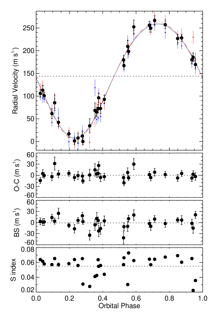
Figure 1.— Orbital solution for HD 285507b. The panels, from top to bottom, show the relative RVs, best-fit residuals, bisector span variations, and relative S index values. In the top panel the large black points are the final RVs, but also plotted are the RVs derived from the blue and red orders of the spectrum, showing agreement at different wavelengths (see Section 3.4). RV error bars represent the internal errors, and do not include astrophysical or instrumental jitter, although $7.2~{}{\rm m\thinspace s^{-1}}$ instrumental jitter was added to the orbital fit. The solid black curve shows the best-fit orbital solution (and the blue and red dashed curves show the fits to the blue and red RVs). The blue curve is nearly indistinguishable from the black curve. The orbital parameters are listed in Table 3.

3.4. Tests for a False Positive

HD 285507 is slowly rotating ($P_{\rm rot}=11.98$ days; Delorme et al., 2011), no X-ray emission was detected by ROSAT (Stern et al., 1995), and no stellar jitter term was required to obtain a good fit to the radial velocities, all of which are suggestive of a chromospherically inactive star. Nevertheless, to rule out false positive scenarios in which the observed RV variations are caused by stellar activity or stellar companions, we used our observations of HD 285507 to search for spectroscopic signatures that correlate with the orbital period.

If the RV variations were caused by a background blend (Mandushev et al., 2005) or star spots (Queloz et al., 2001), we would expect the shape of the star’s line bisector to vary in phase with the radial velocities. A standard prescription for characterizing the shape of a line bisector is to measure the relative velocity at its top and bottom; this difference is referred to as a line bisector span (see, e.g., Torres et al., 2005). To test against background blends or star spots, we computed the line bisector spans for all observations of HD 285507. As illustrated in Figure 1, the bisector span variations are small ($\sigma_{\rm BS}=15~{}{\rm m\thinspace s^{-1}}$) and they are not correlated with the observed RV variations, having a Pearson r value of only $0.06$.

For each spectrum we also computed the S index — an indicator of chromospheric activity in the Ca ii H&K lines. We follow the procedure of Vaughan et al. (1978), but we note that our S indices are not calibrated to their scale; these are relative measurements. Correlation between S index and orbital phase might be expected if the apparent RV variations were activity-induced, but as shown in Figure 1, there is no such correlation (Pearson $r=0.17$). Instead, there may be significant periodicity in the S indices at $12$ or $13$ days (Figure 2), which is similar to the published rotation period of $11.98$ days. Our data set is too sparse to claim a detection of the rotation period from the activity measurement, but we can see there is no power at the observed orbital period of $6.088$ days.

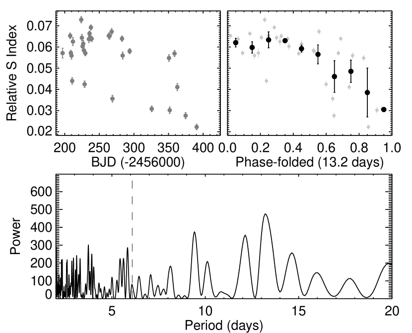
Figure 2.— Top left: the stellar activity, as characterized by the relative S index measured from our spectra of HD 285507. Bottom: the Lomb–Scargle periodogram indicates that there may be significant periodicity on timescales similar to the stellar rotation period of $11.98$ days (Delorme et al., 2011), but not at the RV period of $6.09$ days (dashed line). Top right: the data have been folded onto the highest peak, $13.2$ days, and binned for illustration.

Finally, if spots were the source of the variation, we might also expect the RV amplitude to be wavelength dependent because contrast between the spot and the stellar photosphere is wavelength dependent. We derived RVs for the blue and red orders separately (weighted mean wavelengths of $\lambda_{\rm blue}=4967$ Å and $\lambda_{\rm red}=5845$ Å), and find the amplitudes to be consistent at the level of $0.5\sigma$ ($3~{}{\rm m\thinspace s^{-1}}$, Figure 1). This agreement between the red and blue amplitudes is encouraging, but is not conclusive by itself. We generally expect large amplitude differences between the optical and infrared for spot-induced RVs because the spot contrast can change drastically over that wavelength range. The expected amplitude difference for our smaller ($\mathord{\sim}1000$ Å) wavelength span, on the other hand, is more uncertain because the local wavelength dependence of the RV amplitudes is itself dependent upon the (unknown) temperature difference between spot and photosphere (e.g., Reiners et al., 2010; Barnes et al., 2011). The simulations of Reiners et al. (2010) indicate that the amplitude difference might be detectable if the spot contrast is low, but not if it is high. Even this is not certain, though, as other authors (Desort et al., 2007) predict a $10\%$ drop in amplitude between blue and red for high contrast spots on solar-type stars. Regardless, from these results and the work of Saar & Donahue (1997), we estimate that to induce the observed RV amplitude ($125~{}{\rm m\thinspace s^{-1}}$) given $v\sin{i}\approx 3.2~{}{\rm km\thinspace s^{-1}}$, the spot would have to cover $\mathord{\sim}20\%$ of the visible stellar surface for low contrast spots ($\Delta_{T_{\rm eff}}\approx 200$ K) or $\mathord{\sim}5\%$ for high contrast spots ($\Delta_{T_{\rm eff}}\approx 1500$ K). Large and high contrast spots are more likely to appear on very magnetically active stars (e.g., Bouvier et al., 1995), and we have no evidence for strong magnetic activity. Furthermore, for such spot configurations, the RV-bisector correlation should be strong (e.g., Mahmud et al., 2011), and we observe no correlation.

We conclude from the evidence presented above that the observed RV variation is not caused by spots, but is the result of an orbiting planetary companion.

3.5. Stellar and Planetary Properties

We used the spectroscopic classification technique Stellar Parameter Classification (SPC; Buchhave et al., 2012) to determine the effective temperature $T_{\rm eff}$, surface gravity $\log{g}$, projected rotational velocity $v\sin{i}$, and metallicity [m/H] of HD 285507. In essence, SPC cross-correlates an observed spectrum against a grid of synthetic spectra, and uses the correlation peak heights to fit a $3$-dimensional surface in order to find the best combination of atmospheric parameters ($v\sin{i}$ is fit iteratively since it is only weakly correlated to changes in the other parameters). We used the CfA library of synthetic spectra, which are based on Kurucz model atmospheres (Kurucz, 1992) calculated by John Laird for a linelist compiled by Jon Morse. Like other spectroscopic classification techniques, SPC can be limited by degeneracy between parameters, notably $T_{\rm eff}$, $\log{g}$, and [m/H], but in this case we can enforce the known cluster metallicity ($+0.13\pm 0.01$, Paulson et al., 2003) to partially break that degeneracy.

To determine the physical stellar parameters, we utilized the Dartmouth (Dotter et al., 2008), Yonsei-Yale (Yi et al., 2001), and Padova (Girardi et al., 2000) stellar models. Applying an observational constraint on the size of the star — imposed indirectly by the spectroscopic $T_{\rm eff}$, $V$ magnitude ($V=10.473\pm 0.012$, Röser et al., 2011), and distance ($41.34\pm 3.61$ pc; van Leeuwen, 2007) — and enforcing the age ($625$ Myr; Perryman et al., 1998) and metallicity of the Hyades, we determined the best fit mass and radius for each of the three isochrones. All three results agreed to within $3\%$ in mass and $5\%$ in radius, and although the resulting $\log{g}$ values indicated by the isochrones were consistent with the spectroscopically determined value, the temperatures were nominally discrepant at the $2\sigma$ level. It is possible that, for stars of this mass and age, the stellar models and/or SPC suffer from a systematic bias not reflected in the formal errors. Given that the exact stellar parameters have little bearing on the results presented in this paper, we choose to simply caution the reader and inflate the errors on stellar mass and radius by a factor of two. We adopted the mean mass and radius from the three isochrone fits ($M_{*}=0.734\pm 0.034~{}{M_{\odot}}$, $R_{*}=0.656\pm 0.054~{}{R_{\odot}}$), where the uncertainties listed here are the inflated statistical errors. Table 3 lists all of the stellar and planetary properties. We note that our adopted temperature ($4503$ K) is consistent with previous estimates of the spectral type (e.g., K5, Nesterov et al., 1995), and using the spectral type/temperature relations assembled in Kraus & Hillenbrand (2007), we estimate a more precise spectral type of HD 285507 to be K4.5.

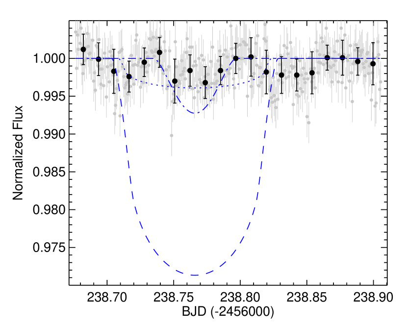
Figure 3.— Light curve of HD 285507, showing the individual data (small gray circles), the binned data (large black circles), and three simulated transit models at the predicted time of transit (all of which are rejected as bad fits to the data): a central transit of a $0.95~{}{R_{\rm Jup}}$ planet (dashed line), a central transit of a $0.35~{}{R_{\rm Jup}}$ planet (dotted line), and a grazing transit ($b=1$) of a $0.95~{}{R_{\rm Jup}}$ planet (dash-dotted line). The latter two cases mark simulated detection limits for the observed data quality (see Section 4). The uncertainty in the time of conjunction at this epoch is only about $1$ hr ($\mathord{\sim}0.04$ days).

4. Stellar Inclination and a Search for Transits

Since the rotation period of HD 285507 is $11.98$ days and we have estimates for $R_{*}$ and $v\sin{i}$, we can in principle calculate the inclination of the stellar spin axis. In practice, the fractional uncertainty on $v\sin{i}$ is large (not because the absolute uncertainty is large, but because the value is small), and the inclination can only be constrained to be $i>72^{\circ}$. This does not exclude an edge-on stellar equator ($i=90^{\circ}$), and because hot Jupiters orbiting cool stars ($\lesssim 6250$ K) tend to be well-aligned with the stellar spin axis (see, e.g., Albrecht et al., 2012), an inclination of $\mathord{\sim}90^{\circ}$ would make a transit more likely a priori. However, even an inclined stellar spin axis would not preclude transits of HD 285507, as there is evidence to suggest that young planets tend to be more misaligned than old planets (e.g., Triaud, 2011). In addition to providing a radius measurement for HD 285507b, transits of this relatively young planet orbiting a cool star could be valuable to the interpretation of these intriguing correlations.

With this in mind, we conducted photometric monitoring of HD 285507 with KeplerCam on the FLWO $1.2$ m telescope at the predicted time of conjunction on UT 2012 November 7. KeplerCam is a monolithic, 4k$\times$4k Fairchild 486 chip with a $23^{\prime}\times 23^{\prime}$ FOV and a resolution of $0.^{\prime\prime}336~{}{\rm pixel}^{-1}$. We used a Sloan $i$ filter with exposure times of $45$ s and readout time of $12$ s, obtaining a total of $334$ images over $5.5$ hours. We reduced the raw images using the IRAF package mscred, and performed aperture photometry with SExtractor (Bertin & Arnouts, 1996).

The resulting light curve showed no sign of a transit, but to determine our detection sensitivity, we simulated transits — using the routines of Mandel & Agol (2002) and a quadratic limb darkening law from Claret et al. (2012) — and injected them into our observed data. For each injected transit, we compared the mean flux in transit (for all points between mid-ingress and mid-egress) to the mean flux out of transit. If the two differed by more than $1\sigma$, we classified that transit as detected. From this, we can rule out a central transit of objects larger than $0.35~{}{R_{\rm Jup}}$ (see Figure 3). If HD 285507b were to transit, then the derived minimum mass would be the true planetary mass. Under this assumption and using the mass-radius-flux relation from Weiss et al. (2013), we would then expect its radius to be $\mathord{\sim}0.95~{}{R_{\rm Jup}}$, much larger than our sensitivity limit. We can also rule out all transits of a $0.95~{}{R_{\rm Jup}}$ planet with impact parameters $b<1$ (i.e., all but the most extreme grazing transits). Using the final ephemeris, the transit center should have occurred $2.22$ hr after our observations began ($T_{\rm c}=2456238.7686$ BJD), with an uncertainty of $\mathord{\sim}1$ hr, so it is unlikely that a transit occurred outside our observing window.

5. Evidence for Dynamical Scattering of HD 285507b

The discovery of a hot Jupiter in the Hyades open cluster brings the total number of short period giant planets in clusters to $3$. Of these, however, HD 285507b is unique in that it is the only one that is definitively eccentric; the two planets in Praesepe are consistent with having circular orbits. As described in the introduction, the non-zero eccentricity of HD 285507b could be a tracer of its migration history if the planet is dynamically young (i.e., $\tau_{\rm cir}>t_{\rm age}=625$ Myr). If it is dynamically old, then the orbit should have already circularized, and establishing a credible link between the eccentricity and the migration process becomes more difficult. In planet–planet scattering for example, if the outer planet gets ejected during the scattering event as is expected, then one must invoke a separate mechanism to excite eccentricity again after circularization. To put it differently, if HD 285507b is dynamically young, then planet–planet scattering is sufficient (but not necessary) to explain the observations; if the planet is dynamically old, planet–planet scattering is neither sufficient nor necessary. To test these scenarios, we estimate $\tau_{\rm cir}$ using the equation given by Adams & Laughlin (2006):

$$\tau_{\rm cir}= ~{}1.6~{}{\rm Gyr}\times\left(\frac{Q_{\rm P}}{10^{6}}\right)\times\left(\frac{M_{\rm P}}{M_{\rm Jup}}\right)\times\left(\frac{M_{*}}{{M_{\odot}}}\right)^{-1.5}$$

$$\times\left(\frac{R_{\rm P}}{R_{\rm Jup}}\right)^{-5}\times\left(\frac{a}{0.05~{}{\rm AU}}\right)^{6.5}$$ (1)

where $Q_{\rm P}$ is the planetary tidal quality factor (a measure of the efficiency of tidal dissipation within the planet). Note that $\tau_{\rm cir}$ scales linearly with $Q_{\rm P}$, which is unknown to within an order of magnitude. The Jupiter–Io interaction does provide the constraint $6\times 10^{4}<Q_{\rm Jup}<2\times 10^{6}$ (Yoder & Peale, 1981), but $Q_{\rm P}$ is likely dependent upon temperature, composition, rotation, and internal structure, all of which may be quite different for hot Jupiters. $Q_{\rm P}\approx 10^{6}$, which we adopt herein, is a fiducial value often assumed for short period giant planets (for a more detailed discussion of tidal dissipation, see, e.g., Ogilvie & Lin, 2004).

Since HD 285507b does not transit, we do not know $R_{\rm P}$ and measure only a minimum mass, $M_{\rm P}\sin{i}$. However, we can calculate the expectation value of $\sin{i}$ for randomly oriented orbits to determine the most likely mass, and then use the giant planet mass–radius–flux relation derived by Weiss et al. (2013) to estimate the planetary radius:

$$\frac{R_{\rm P}}{R_{\oplus}}=2.45~{}\left(\frac{M_{\rm P}}{M_{\oplus}}\right)^{-0.039}\left(\frac{F}{{\rm erg~{}s^{-1}~{}cm^{-2}}}\right)^{0.094}$$ (2)

where $F$ is the time-averaged incident flux on the planet. Since $R_{\rm P}$ depends only weakly on $M_{\rm P}$, assuming an inclination is not likely to introduce a large radius error — there is only a $1\%$ difference in derived radius between edge-on and average-inclination orientations.

Under these assumptions, we find $\tau_{\rm cir}\approx 11.8$ Gyr — much larger than the age of the cluster. Note that this holds true even for the full range of $Q_{\rm Jup}$ (corresponding to $700~{}{\rm Myr}<\tau_{\rm cir}<22.6$ Gyr). We conclude that HD 285507b is dynamically young. While it is tempting to thus proclaim that migration has occurred via a HEM mechanism, recall that this is not a necessary condition for a dynamically young planet with an eccentric orbit. For any individual planet, non-zero eccentricity could also be the result of continued interaction with an undetected planetary or stellar companion, a recent close stellar encounter, or even modest eccentricity excitation via Type II migration (e.g., D’Angelo et al., 2006). Only analysis of a population of planets can provide meaningful insight into the migration process in this manner. Therefore, we turn to the literature for ages and circularization timescales of the known sample of hot Jupiters.

6. Evidence for Dynamical Scattering Among Known Exoplanets

6.1. Description of the Analysis

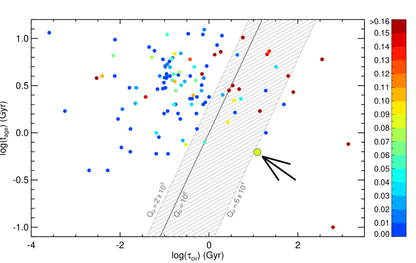
Figure 4.— Age vs. circularization timescale for short period ($P<10$ days) massive ($M>0.3~{}{M_{\rm Jup}}$) planets, assuming a tidal quality factor $Q_{\rm P}=10^{6}$ for all planets. The solid dark line indicates where $t_{\rm age}=\tau_{\rm cir}$; planets to the left of the line are expected to have undergone tidal circularization. We also plot a shaded region to show the estimated uncertainty in this boundary given the range of $Q_{\rm P}$ values consistent with observations of the Jupiter–Io interaction (see Yoder & Peale, 1981). The data points are colored according to their eccentricity, and HD 285507b is the large outlined circle indicated by the arrow. There is a hint that the right side is populated by preferentially eccentric (red) planets and the left side by preferentially circular (blue) planets. This is explored further in Figure 5.

To search for dynamical imprints of migration among known hot Jupiters ($M_{\rm P}>0.3~{}{M_{\rm Jup}}$, $P<10$ days), we follow the prescription described above to calculate $\tau_{\rm cir}$ (and $M_{\rm P}$ and $R_{\rm P}$ for non-transiting planets). We adopt ages, eccentricities, planetary masses and radii, and stellar masses, radii, and temperatures from the literature. In Figure 4, we plot $t_{\rm age}$ versus $\tau_{\rm cir}$ for this sample. While the figure is complicated by the uncertainties already discussed as well as poorly constrained ages and potential biases in measuring modest eccentricities (e.g., Shen & Turner, 2008; Pont et al., 2011; Zakamska et al., 2011; Wang & Ford, 2011), there is a hint that the points to the right of the circularization boundary are preferentially eccentric and the ones to the left are preferentially circular. If HEM were responsible for the final stages of hot Jupiter migration, this would be expected; planets get scattered inward on highly eccentric orbits and circularize over time. If Type II migration were responsible, we should expect very little difference between the eccentricity distributions to the right and left of the boundary; ordered migration through a gas disk should largely preserve circular orbits, so subsequent tidal interactions would not change the population significantly. In Figure 5, we plot the eccentricity histograms and cumulative distributions for the two populations, which contain $92$ and $22$ planets (as shown in Figure 4). To quantify the difference between them, we ran a Kolmogorov–Smirnov (KS) test. The KS $p$-value is the likelihood that the two subsamples came from the same parent distribution, and in this case, $p=3.3\times 10^{-5}$. We conclude that the two distributions do not come from the same parent distribution, with $\mathord{\sim}99.997\%$ confidence, and infer that high eccentricity migration mechanisms play a significant role in hot Jupiter migration. We also ran an Anderson–Darling (AD) test, which is similar to a KS test, but is more sensitive to differences in the distribution tails. The AD test indicates an even greater significance that the two distributions do not come from the same parent distribution of eccentricities.

6.2. The Effect of Measurement Errors

As noted previously, ages and eccentricities can be difficult to determine for many of these systems, so it is important to consider what effect uncertainties may have on the significance of our result. Ages of field stars can be estimated by many techniques, including gyrochronology, stellar activity, lithium abundance, and isochrone fitting. However, ages derived from multiple techniques do not always agree, and when they do agree, the allowed range of ages can still be quite large. Likely for this reason, The Extrasolar Planets Encylcopaedia does not report uncertainties on the age (when age is reported at all). Mamajek & Hillenbrand (2008) claim a precision of $\mathord{\sim}0.2$ dex in their activity–age relation, and while not all stars in this sample have ages derived in this manner, we believe this to be an appropriate approximate error for isochrone fitting as well, which is one of the more widespread techniques employed to determine ages. We therefore adopt this as a typical error in our analysis.

Eccentricity errors are similarly heterogeneously reported in the literature, especially for nearly circular orbits. Some authors assume zero eccentricity in such cases for simplicity, which introduces a bias toward smaller values, while others report upper limits or a measured eccentricity. When a small measured value is reported, it may be biased toward larger eccentricities depending on the details of the fitting. Rather than worry about potential conflicting biases in a heterogeneous set of eccentricities and associated errors, we assume a constant eccentricity error of $0.05$ for all planets in our sample. We also assume errors of $10\%$ on stellar and planetary masses and radii, $3\%$ on semi-major axis, and $100$ K on stellar effective temperature. These values are minor contributors to uncertainty in the analysis, but they do have a small effect on the derived circularization timescales.

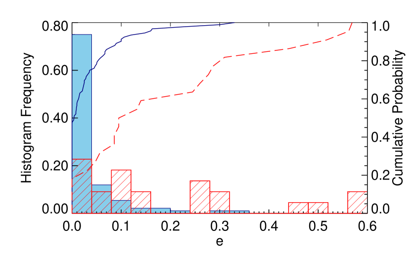
Figure 5.— Eccentricity histograms and cumulative distributions of hot Jupiters that have (filled blue; left of the thick solid line in Figure 4) and have not (striped red; right of the line) been tidally circularized. As in Figure 4, we have assumed $Q_{\rm P}=10^{6}$ for all planets. A KS test rejects the hypothesis that the two subsamples are drawn from the same distribution with $99.997\%$ confidence.

Using the above errors, we redraw our sample $10^{4}$ times. For each of these simulated data sets, we run a KS test to determine the significance of the difference in populations, resulting in a distribution of $10^{4}~{}p$-values. The median of this distribution is $2.7\times 10^{-4}$, or a $99.973\%$ confidence (nearly $4\sigma$) that the two samples come from different parent distributions. Furthermore, we find that even for eccentricity errors as large as $0.1$ (which is unrealistically large for nearly all planets in the sample), the KS significance remains greater than $3\sigma$. From this, we conclude that even with conservatively large errors, our result holds: dynamically young planets have larger eccentricities, which suggests HEM mechanisms contribute significantly to hot Jupiter migration.

7. A Constraint on the Tidal Quality Factor $Q$ for Hot Jupiters

Until now we have been assuming $Q_{\rm P}=10^{6}$ to determine which planets are dynamically young (right side of the circularization boundary in Figure 4) and which are dynamically old (left side), allowing us to draw conclusions about the migration process. If we instead start with the assumption that planets migrate inward in possession of some intial eccentricity (rather than being gently shepherded on circular orbits through the gas disk), we can invert the problem to place a constraint on the tidal quality factor $Q_{\rm P}$. As we vary $Q_{\rm P}$, the circularization boundary changes location, and the difference between the two populations should be maximized (and the KS $p$-value minimized) for the correct (average) hot Jupiter $Q_{\rm P}$. Note that it does not matter what fraction of hot Jupiters has undergone HEM – if any fraction has, then the minimum $p$-value should occur when the circularization boundary is in the correct place.

Figure 6 shows the results of this experiment. A value on the order of $10^{6}$ is preferred, which seems to rule out much of the parameter space consistent with Jupiter’s tidal quality factor (and validates our assumption of $Q_{\rm P}=10^{6}$). The discrete data points do not produce a smooth distribution, so finding the minimum is not straightforward. As such, we smooth it using a moving average with a boxcar filter of size [$\frac{2}{3}Q_{\rm P},\frac{3}{2}Q_{\rm P}$]. Quantitative confidence limits on the minimum are difficult to assess (the vertical axis is not a probability associated directly with $Q_{\rm P}$), but we take approximate upper and lower limits on $Q_{\rm P}$ to be those for which the smoothed p-value is $10$ times its smoothed minimum value, which occurs for $Q_{\rm P}=1.39\times 10^{6}$. For each simulated data set described in Section 6.2, we calculate $Q_{\rm P}$ this way and find the median to be similar ($1.12\times 10^{6}$), but with smaller errors. This is not surprising, as the statistical errors from the simulations are akin to a standard deviation of the mean whereas the errors derived from a single p-value versus $Q_{\rm P}$ experiment are akin to a sample standard deviation. To describe the population, we therefore adopt the latter and suggest an appropriate tidal quality factor for a typical hot Jupiter is $\log{Q_{\rm P}}=6.14^{+0.41}_{-0.25}$ (see Figure 6 for a visual representation).

8. Summary and Conclusions

Our discovery of a hot Jupiter in the Hyades bolsters the statistics of short period giant planets in open clusters (of which three are now known). Including the Paulson et al. (2004) null result in the Hyades ($0$ planets among $74$ FGK stars), our Hyades sample ($1$ in $26$), and an updated census of Praesepe including unpublished data from our second year of observations ($2$ in $60$), a total of $3$ out of $160$ stars host a hot Jupiter. After correcting for completeness and calculating Poisson errors following the prescription in Gehrels (1986), we find a hot Jupiter frequency of $1.97^{+1.92}_{-1.07}\%$ in the metal-rich Praesepe and Hyades open clusters. However, giant planet occurrence scales with metallicity approximately as $10^{2{\rm[Fe/H]}}$ (Fischer & Valenti, 2005). If we take ${\rm[Fe/H]}\approx+0.15$ as representative of the combined Praesepe and Hyades sample, the solar-metallicity-adjusted hot Jupiter frequency in clusters is $0.99^{+0.96}_{-0.54}\%$. Although more discoveries are needed to reduce the uncertainty, this is in good agreement with the frequency for field stars ($1.20\pm 0.38\%$; Wright et al., 2012), and improves the evidence that planet frequency is the same in clusters and the field.

A primary motivation for the search for young planets is that their ages are comparable to the timescale of migration. Thus, the orbital properties of such planets may still bear the dynamical signature of this process. Since different migration mechanisms are predicted to produce hot Jupiters on different timescales and with different orbital eccentricities, we can use the properties of young hot Jupiters (and their existence at various ages) to determine the process by which they migrate. The ages of the cluster planets discovered thus far do not place a strong direct constraint on the timescale of migration (we know only that the process took less than $600$ Myr), but the newly discovered planet in the Hyades holds a clue its dynamical history. HD 285507b has a long circularization timescale, so its non-zero eccentricity may be a remnant of the migration process, which would suggest planet-planet scattering or Kozai cycles have played a role in its orbital evolution. There is no observational evidence for a third body, but one cannot be excluded either. The RV timespan is not long enough to rule out a second giant planet (which also could have been ejected during scattering), and imaging by Patience et al. (1998) only rules out companions more massive than $0.13~{}{M_{\odot}}$ with projected separations $5$–$50$ AU.

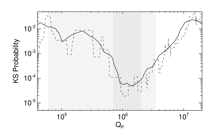
Figure 6.— KS $p$-values from comparisons of the eccentricity distributions of hot Jupiter systems with $t_{\rm age}<\tau_{\rm cir}$ to those with $t_{\rm age}>\tau_{\rm cir}$, as a function of the assumed $Q_{\rm P}$ (dashed line); the solid line shows the same result after a boxcar filtering. Since the minimum $p$-value should occur for the most realistic $Q_{\rm P}$ (see Section 7), we can constrain $Q_{\rm P}$ for a typical hot Jupiter to be between about $7.8\times 10^{5}$ and $3.5\times 10^{6}$ (right shaded region encompassing the broad minimum). The Jupiter–Io constraint (left shaded region) only overlaps partially with the position of the minimum at $Q_{\rm P}=1.39\times 10^{6}$, and given the expectation that $Q$ will be larger for hot Jupiters, we do not apply this constraint to our adopted range for $Q_{\rm P}$.

Applying this idea more broadly, we have compared ages and circularization timescales for all known hot Jupiters and find evidence for two families of planets, distinguished by their orbital properties: (1) mostly circular orbits for the “dynamically old” planets, those with $\tau_{\rm cir}<t_{\rm age}$, and (2) a range of eccentricities for “dynamically young” planets, those with $\tau_{\rm cir}>t_{\rm age}$. If Type II migration were the leading driver of hot Jupiter migration, both dynamically young and old planets should have circular orbits. We thus conclude that HEM is important for producing hot Jupiters. However, we can only say that these planets have experienced dynamical stirring at some point, and do not suggest that this evidence shows Type II migration to be unimportant. On the contrary, as shown by simulations time and again, Type II migration is almost certainly important to orbital evolution before the gas disk dissipates, but we suggest that for a large fraction of hot Jupiter systems, planet-planet scattering or the Kozai mechanism is responsible for the final stages of inward migration. A larger sample of dynamically young (non-circularized) planets may allow us to determine what that fraction is. Since few hot Jupiters have circularization timescales greater than $1$ Gyr, a good way to enhance this sample is to continue finding young planets.

That HEM mechanisms play an important role in hot Jupiter migration has already been suggested, and is supported by a rich data set of stellar obliquity measurements in hot Jupiter systems (see Albrecht et al., 2012, for a recent discussion). In addition to the excitation of orbital eccentricity, dynamical encounters with a third body are expected to produce a range of orbital inclinations, although tidal interactions with the host star may realign the systems over time. These inclinations can be measured precisely, most notably via the Rossiter–McLaughlin effect (Rossiter, 1924; McLaughlin, 1924), and the results of such studies parallel those presented in this paper: systems for which the tidal timescale is short tend to be well-aligned, and those for which the timescale is long display high obliquities. Albrecht et al. (2012) do caution that stars and their disks may be primordially misaligned for reasons unrelated to hot Jupiters, but we see no obvious reason for this to influence the eccentricities. Migration through multi-body dynamical interactions, on the other hand, could explain both the inclined orbits and high eccentricities observed in systems that have not yet experienced significant tidal interactions. Whether that process is primarily planet-planet scattering or the Kozai effect remains to be determined, and it is likely that more data will be needed to properly answer this question.

Finally, the tidal circularization boundary that separates the dynamically young and old populations of hot Jupiters is sensitive to the choice of the planetary tidal quality factor, $Q_{\rm P}$, so we have leveraged this dependence to constrain the typical value for hot Jupiters to be $\log{Q_{\rm P}}=6.14^{+0.41}_{-0.25}$. $Q_{\rm P}$ has wide-ranging implications, e.g., for simulating orbital evolution (Beaugé & Nesvorný, 2012) or modeling the inflated radii of hot Jupiters (Bodenheimer et al., 2003), but has thus far proven difficult to constrain observationally. While our result still includes substantial uncertainty and will not be applicable to any one planet, it can be applied to these problems in a statistical sense. Moreover, it offers a path forward: as our sample of longer period and young hot Jupiters grows, the determination of $Q_{\rm P}$ using this method should improve.

References

- Adams & Laughlin (2006) Adams, F. C., & Laughlin, G. 2006, ApJ, 649, 1004
- Albrecht et al. (2012) Albrecht, S., Winn, J. N., Johnson, J. A., et al. 2012, ApJ, 757, 18
- Bailey et al. (2012) Bailey, J. I., III, White, R. J., Blake, C. H., et al. 2012, ApJ, 749, 16
- Barnes et al. (2011) Barnes, J. R., Jeffers, S. V., & Jones, H. R. A. 2011, MNRAS, 412, 1599
- Barnes et al. (2013) Barnes, J. W., van Eyken, J. C., Jackson, B. K., et al. 2013, ApJ, 774, 53
- Beaugé & Nesvorný (2012) Beaugé, C., & Nesvorný, D. 2012, ApJ, 751, 119
- Bertin & Arnouts (1996) Bertin, E., & Arnouts, S. 1996, A&AS, 117, 393
- Bodenheimer et al. (2003) Bodenheimer, P., Laughlin, G., & Lin, D. N. C. 2003, ApJ, 592, 555
- Bouvier et al. (1995) Bouvier, J., Covino, E., Kovo, O., et al. 1995, A&A, 299, 89
- Buchhave et al. (2010) Buchhave, L. A., Bakos, G. Á., Hartman, J. D., et al. 2010, ApJ, 720, 1118
- Buchhave et al. (2012) Buchhave, L. A., Latham, D. W., Johansen, A., et al. 2012, Natur, 486, 375
- Claret et al. (2012) Claret, A., Hauschildt, P. H., & Witte, S. 2012, A&A, 546, 14
- D’Angelo et al. (2006) D’Angelo, G., Lubow, S. H., & Bate, M. R. 2006, ApJ, 652, 1698
- Dawson & Murray-Clay (2013) Dawson, R. I., & Murray-Clay, R. A. 2013, ApJL, 767, L24
- Delorme et al. (2011) Delorme, P., Collier Cameron, A., Hebb, L., et al. 2011, MNRAS, 413, 2218
- Desort et al. (2007) Desort, M., Lagrange, A.-M., Galland, F., et al. 2007, A&A, 473, 983
- Dong et al. (2014) Dong, S., Katz, B., & Aristotle, S. 2014, ApJL, 781, L5
- Dotter et al. (2008) Dotter, A., Chaboyer, B., Jevremović, D., et al. 2008, ApJS, 178, 89
- Fabrycky & Tremaine (2007) Fabrycky, D., & Tremaine, S. 2007, ApJ, 669, 1298
- Fischer & Valenti (2005) Fischer, D. A., & Valenti, J. 2005, ApJ, 622, 1102
- Ford & Rasio (2008) Ford, E. B., & Rasio, F. A. 2008, ApJ, 686, 621
- Fressin et al. (2013) Fressin, F., Torres, G., Charbonneau, D., et al. 2013, ApJ, 766, 81
- Fűrész (2008) Fűrész, G. 2008, PhD thesis, Univ. of Szeged, Hungary
- Gehrels (1986) Gehrels, N. 1986, ApJ, 303, 336
- Girardi et al. (2000) Girardi, L., Bressan, A., Bertelli, G., & Chiosi, C. 2000, A&AS, 141, 371
- Goldreich & Tremaine (1980) Goldreich, P., & Tremaine, S. 1980, ApJ, 241, 425
- Haisch et al. (2001) Haisch, K. E., Jr., Lada, E. A., & Lada, C. J. 2001, ApJL, 553, L153
- Hartman et al. (2009) Hartman, J. D., Gaudi, B. S., Holman, M. J., et al. 2009, ApJ, 695, 336
- Juric & Tremaine (2008) Juric, M., & Tremaine, S. 2008, ApJ, 686, 603
- Kennedy & Kenyon (2008) Kennedy, G. M., & Kenyon, S. J. 2008, ApJ, 673, 502
- Kraus & Hillenbrand (2007) Kraus, A. L., & Hillenbrand, L. A. 2007, AJ, 134, 2340
- Kurucz (1992) Kurucz, R. L. 1992, in IAU Symp. 149, The Stellar Populations of Galaxies, ed. B. Barbuy & A. Renzini (Dordrecht: Kluwer), 225
- Lin & Papaloizou (1986) Lin, D. N. C., & Papaloizou, J. 1986, ApJ, 309, 846
- Mahmud et al. (2011) Mahmud, N. I., Crockett, C. J., Johns-Krull, C. M., et al. 2011, ApJ, 736, 123
- Mamajek & Hillenbrand (2008) Mamajek, E. E., & Hillenbrand, L. A. 2008, ApJ, 687, 1264
- Mandel & Agol (2002) Mandel, K., & Agol, E. 2002, ApJL, 580, L171
- Mandushev et al. (2005) Mandushev, G., Torres, G., Latham, D. W., et al. 2005, ApJ, 621, 1061
- Martin & Livio (2013) Martin, R. G., & Livio, M. 2013, MNRAS, 434, 633
- Mayor & Queloz (1995) Mayor, M., & Queloz, D. 1995, Natur, 378, 355
- Mayor et al. (2011) Mayor, M., Marmier, M., Lovis, C., et al. 2011, A&A, submitted (arXiv:1109.2497)
- McLaughlin (1924) McLaughlin, D. B. 1924, ApJ, 60, 22
- Meibom et al. (2011) Meibom, S., Barnes, S. A., Latham, D. W., et al. 2011, ApJL, 733, L9
- Meibom et al. (2013) Meibom, S., Torres, G., Fressin, F., et al. 2013, Natur, 499, 55
- Mochejska et al. (2006) Mochejska, B. J., Stanek, K. Z., Sasselov, D. D., et al. 2006, AJ, 131, 1090
- Nesterov et al. (1995) Nesterov, V. V., Kuzmin, A. V., Ashimbaeva, N. T., et al. 1995, A&AS, 110, 367
- Nidever et al. (2002) Nidever, D. L., Marcy, G. W., Butler, R. P., et al. 2002, ApJS, 141, 503
- Ogilvie & Lin (2004) Ogilvie, G. I., & Lin, D. N. C. 2003, ApJ, 610, 477
- Pasquini et al. (2012) Pasquini, L., Brucalassi, A., Ruiz, M. T., et al. 2012, A&A, 545, 139
- Patience et al. (1998) Patience, J., Ghez, A. M., Reid, I. N., et al. 1998, AJ, 115, 1972
- Paulson et al. (2004) Paulson, D. B., Cochran, W. D., & Hatzes, A. P. 2004, AJ, 127, 3579
- Paulson et al. (2003) Paulson, D. B., Sneden, C., & Cochran, W. D. 2003, AJ, 125, 3185
- Pels et al. (1975) Pels, G., Oort, J. H., & Pels-Kluyver, H. A. 1975, A&A, 43, 423
- Pepper et al. (2008) Pepper, J., Stanek, K. Z., Pogge, R. W., et al. 2008, AJ, 135, 907
- Perryman et al. (1998) Perryman, M. A. C., Brown, A. G. A., Lebreton, Y., et al. 1998, A&A, 331, 81
- Pont et al. (2011) Pont, F., Husnoo, N., Mazeh, T., & Fabrycky, D. 2011, MNRAS, 414, 1278
- Queloz et al. (2001) Queloz, D., Henry, G. W., Sivan, J. P., et al. 2001, A&A, 379, 279
- Quinn et al. (2012) Quinn, S. N., White, R. J., Latham, D. W., et al. 2012, ApJL, 756, L33
- Rasio & Ford (1996) Rasio, F. A., & Ford, E. B. 1996, Sci, 274, 954
- Reiners et al. (2010) Reiners, A., Bean, J. L., Huber, K. F., et al. 2010, ApJ, 710, 432
- Röser et al. (2011) Röser, S., Schilbach, E., Piskunov, A. E., et al. 2011, A&A, 531, 92
- Rossiter (1924) Rossiter, R. A. 1924, ApJ, 60, 15
- Saar & Donahue (1997) Saar, S. H., & Donahue, R. A. 1997, ApJ, 485, 319
- Shen & Turner (2008) Shen, Y., & Turner, E. L. 2008, ApJ, 685, 553
- Socrates et al. (2012) Socrates, A., Katz, B., Dong, S., & Tremaine, S. 2012, ApJ, 750, 106
- Stauffer et al. (1998) Stauffer, J. R., Schultz, G., & Kirkpatrick, J. D. 1998, ApJL, 499, L199
- Stern et al. (1995) Stern, R. A., Schmitt, J. H. M. M., & Kahabka, P. T. 1995, ApJ, 448, 683
- Struve (1952) Struve, O. 1952, Obs, 72, 199
- Torres et al. (2005) Torres, G., Konacki, M., Sasselov, D. D., & Jha, S. 2005, ApJ, 619, 558
- Triaud (2011) Triaud, A. H. M. J. 2011, A&A, 534, 6
- van Altena (1966) van Altena, W. F. 1966, AJ, 71, 482
- van Bueren (1952) van Bueren, H. G. 1952, BAN, 11, 385
- van Eyken et al. (2012) van Eyken, J. C., Ciardi, D. R., von Braun, K., et al. 2012, ApJ, 755, 42
- van Leeuwen (2007) van Leeuwen, F. 2007, A&A, 474, 653
- van Saders & Gaudi (2011) van Saders, J. L., & Gaudi, B. S. 2011, ApJ, 729, 63
- Vaughan et al. (1978) Vaughan, A. H., Preston, G. W., & Wilson, O. C. 1978, PASP, 90, 267
- Vogt et al. (1994) , Vogt, S. S., Allen, S. L., Bigelow, B. C., et al. 1994, Proc. SPIE, 2198, 362
- Wang & Ford (2011) Wang, J., & Ford, E. B. 2011, MNRAS, 418, 1822
- Weiss et al. (2013) Weiss, L. M., Marcy, G. W., Rowe, J. F., et al. 2013, ApJ, 768, 14
- Winn et al. (2010) Winn, J. N., Johnson, J. A., Howard, A. W., et al. 2010, ApJL, 723, L223
- Wright et al. (2012) Wright, J. T., Marcy, G. W., Howard, A. W., et al. 2012, ApJ, 753, 160
- Yi et al. (2001) Yi, S., Demarque, P., Kim, Y.-C., et al. 2001, ApJS, 136, 417
- Yoder & Peale (1981) Yoder, C. F., & Peale, S. J. 1981, Icar, 47, 1
- Zakamska et al. (2011) Zakamska, N. L., Pan, M., & Ford, E. B. 2011, MNRAS, 410, 1895