Robust Optimal Power Flow with Wind Integration Using Conditional Value-at-Risk
Abstract
Integrating renewable energy into the power grid requires intelligent risk-aware dispatch accounting for the stochastic availability of renewables. Toward achieving this goal, a robust DC optimal flow problem is developed in the present paper for power systems with a high penetration of wind energy. The optimal dispatch is obtained as the solution to a convex program with a suitable regularizer, which is able to mitigate the potentially high risk of inadequate wind power. The regularizer is constructed based on the energy transaction cost using conditional value-at-risk (CVaR). Bypassing the prohibitive high-dimensional integral, the distribution-free sample average approximation method is efficiently utilized for solving the resulting optimization problem. Case studies are reported to corroborate the efficacy of the novel model and approach tested on the IEEE -bus benchmark system with real operation data from seven wind farms.
I Introduction
With the appealing attributes of being environment-friendly and price-competitive over conventional power generation, clean renewable sources of energy, such as wind, solar, hydro, and geothermal energy, have been developing rapidly over the last few decades. Growing at an annual rate of %, wind power generation had GW worldwide installed capacity by the end of [1]. The U.S. Department of Energy set a goal of using wind energy to generate % of the nation’s electricity demand by [2].
Aligned to the goal of boosting the penetration of renewable energy sources in future smart grids, energy management with renewables, including economic dispatch (ED), unit commitment (UC), and optimal power flow (OPF), have been extensively investigated recently. Generally, two types of strategies have been developed to address the key challenge of dealing with the supply-demand balance, which is induced by the stochastic availability and intermittency of renewables. Early works aim at maintaining balance by introducing committed renewable energy. ED penalizing overestimation and underestimation of wind power is investigated in [3]. Worst-case robust distributed dispatch with demand side management is proposed for grid-connected microgrids with distributed energy resources in [4]. Its solution though can be very sensitive to the accuracy of the wind power forecast. For the second type, supply-demand imbalance is allowed up to a certain extent by limiting the loss-of-load probability (LOLP). Leveraging the scenario approximation technique, risk-limiting ED and DC-OPF tasks with correlated wind farms have been developed recently in [5] and [6], respectively. A multi-stage stochastic control problem is pursued for risk-limiting dispatch of wind power in [7]. Chance-constrained two-stage stochastic program is formulated in [8] for UC with uncertain wind power output; see also [9] and [10] for advances in chance-constrained OPF. However, the applied conic optimization technique therein relies on Gaussianity assumptions for the wind power generation.
Additional limitations are present in the aforementioned works. For example, worst-case renewable energy generation is unlikely when it comes to real time operation [4]. The chance-constrained problems are typically non-convex for general probability distributions. Leveraging the scenario sampling, the relaxed convex problems can be solved efficiently. However, in certain scenarios, this technique turns out to be too conservative for scheduling the delivered renewables [5].
This paper deals with robust DC OPF for a smart grid with high penetration of wind power. Instead of a chance-constrained formulation, an optimization problem is introduced with an appropriate regularizer that plays an instrumental role for mitigating the high risk of inadequate wind power. The regularizer is constructed based on the energy transaction cost using the conditional value-at-risk (CVaR). This “smart” CVaR-based regularizer turns out to be capable of utilizing renewables intelligently with limited risk. The resulting optimization problem, which aims at minimizing jointly the generation as well as the energy transaction costs, is provably convex thanks to the CVaR. To bypass the prohibitive high-dimensional integral present in the regularizer, the sample average approximation (SAA) is utilized to obtain an efficient distribution-free approach. Numerical tests are performed on the IEEE -bus benchmark system to corroborate the effectiveness of the novel model and approach using real wind farm data [11], [12], [13].
II Risk Measure: VaR and CVaR
Being the most popular measures of risk, the value-at-risk (VaR) and the conditional value-at-risk (CVaR) play a central role in risk-aware portfolio optimization [14]. These risk metrics were introduced in the ground-breaking works of [15] and [16]. The redux here is useful to grasp the role of these metrics in the present context.
Let the real-valued loss function denote the cost associated with the decision variable ; and the random vector with probability density function supported on a set . In the context of power systems, can represent for instance the power schedules of conventional generators while captures the sources of uncertainty due to e.g., renewables, forecasted load demand, and locational marginal prices (LMPs). The operator-concerned loss represents the cost, which depends on both and . Clearly, the probability of not exceeding a threshold is given by
| (1) |
It can be seen that is the cumulative distribution function (CDF) for the loss parameterized by , which is right continuous and nondecreasing in . Let and denote respectively the -VaR and -CVaR values of the random loss with a prescribed probability level . Commonly chosen values of are, e.g., , , and . Dependent on , the -VaR and -CVaR values are defined as
| (2) | ||||
| (3) |
Since is non-decreasing in , comes out as the left endpoint of the nonempty interval consisting of the solution satisfying . Hence, is the conditional expectation of to be greater than or equal to .
The characterization of and lies in the optimization of a key constructed function
| (4) |
where is the projection operator. The crucial features of relating with are summarized in the following theorem.
Theorem 1 ([15], pp. 24–26).
Function is convex and continuously differentiable in . Furthermore, is convex with respect to while is convex in , provided that is convex in . The relationships among , , and are given as follows
| (5) | ||||
| (6) | ||||
| (7) |
where denotes the left endpoint of the interval set .
It is important to appreciate the claim in Theorem 1 regarding the undesirable characteristics of -VaR, namely non-subadditivity and non-convexity. Theorem 1 asserts that minimizing the convex -CVaR is equivalent to minimizing , which is not only convex, but also easier to approximate. A straightforward and easily implementable approximation of the expectation function is its empirical estimate using Monte Carlo samples , namely
| (8) |
Clearly, the sample average approximation method is distribution free, and the law of large numbers asserts as a good approximation of for large enough. Furthermore, is convex with respect to when is convex in . The non-differentiability due to the projection operator can be readily overcome by leveraging the epigraph form of , which will be shown explicitly in Section III-C.
Leveraging CVaR, a robust OPF problem will be formulated next by considering the transaction cost induced by wind power shortage.
III Robust Optimal Power Flow Formulation
Consider a power grid with buses. Let denote a vector collecting the conventional power outputs of the thermal generators, and the load demand, where denotes transposition. Furthermore, if a renewable energy facility (e.g., a wind farm) is located at bus as well, two quantities will be associated with it: the actual wind power generation , and the power scheduled to be injected to bus . Note that the former is a random variable, whereas the latter is a decision variable. For notational simplicity, define further two -dimensional vectors , and . Clearly, if no generator, load, or wind farm is attached to bus , the th entry of , , or, and is set to zero.
III-A DC Flow Model
For a power transmission network with a total of lines, let denote the reactance associated with the th line. Define further a diagonal matrix , and the branch-bus incidence matrix , such that if its th row corresponds to the branch , then , , and zero elsewhere.
Consider now the DC flow model [17], and let vector collect the nodal voltage phases . Then, the power flows on all transmission lines can be expressed as with . Physical considerations enforce a power flow limit on each transmission line, leading to the line flow constraint
where denotes entry-wise inequality.
Furthermore, flow conservation compels zero net flow at each bus; i.e., the outgoing power flow must equal the aggregate incoming power flows. This gives rise to the nodal balance equation for the DC power flow model:
| (9) |
where is the bus admittance matrix. With denoting the all-ones vector, it holds that , which implies that (9) is invariant to nodal phase shifts. Hence, without loss of generality, the first bus can be set to be the zero phase reference bus, i.e., . For simplicity, only non-dispatchable base loads will be included in . These are fixed constants for the optimization problem that will be formulated later.
Remark 1 (Actual versus committed wind power).
Since day-ahead power dispatch is considered in this paper, power generation schedules should be decided prior to real time operation. Hence, the actual wind power output , which is random due to the wind speed variability, is not available at the decision making time. However, to maintain node balance, slack variables will be introduced to capture the committed wind power injected at the corresponding buses. These are possible to determine before the real time operation, together with other decision variables, namely and .
III-B CVaR-based Energy Transaction Cost
Since the wind generation output is stochastic, it is unlikely that the scheduled power will be equal to the actual one . Thus, in order to satisfy the nodal balance (9) in real time operation, either energy surplus or shortage should be included. In the former case, the wind generation company (W-GENCO) may simply choose to curtail the excess wind power at almost no cost. For the case of shortage, in order to accomplish the bid as promised in its signed day-ahead contract, W-GENCO has then to buy the energy shortfall from the real time market in the form of ancillary services. Generally, wind farms attached to different buses may have different purchase prices. This is simply because they may resort to different energy sellers, or because of the varying real-time LMPs across the grid.
Let denote the purchase transaction cost for the renewable energy facility associated with the th bus. Clearly, with the power shortfall being at bus , the grid-wide total transaction cost is given by . If the general loss function in (4) is replaced by the transaction cost , function related to the conditional expected transaction cost turns out to be
| (10) |
where denotes expectation. The following proposition sheds light on the convexity of .
Proposition 1.
If all costs are convex and non-decreasing, then is convex with respect to .
Proof:
It is worth pointing out that cost functions typically satisfy the condition of Proposition 1. In the simple linear case for which , each constant actually denotes the purchase price at bus . If , then in (10) can be written as
| (11) |
It is now possible to formulate the robust DC-OPF task with the CVaR-based transaction cost, as in the ensuing section.
III-C Problem Statement
Let be the generation cost associated with the th thermal generator. Function is chosen convex, typically quadratic or piecewise linear. The robust DC-OPF problem amounts to minimizing the conventional generation cost, as well as the CVaR-based transaction cost under certain physical grid operation constraints; that is,
| (12a) | ||||
| s.t. | (12b) | |||
| (12c) | ||||
| (12d) | ||||
| (12e) | ||||
| (12f) | ||||
where the risk-aversion parameter controls the trade off between the generation cost and the transaction cost, which should be pre-determined based on the operator’s concern. Besides constraints (12b) – (12d), constraints (12e) and (12f) entail the physical limits of and , respectively, namely and . Only a single scheduling period is considered here. However, (12) can be readily extended to formulate multi-period dispatch with time coupling constraints, e.g., ramping up/down rates and unit minimum-up/down constraints (see e.g., [8]).
Alternatively, it is reasonable to consider a CVaR-constrained problem, which minimizes the generation cost with a constraint to ensure that the conditional expected transaction cost is no more than a given budget . The corresponding problem formulation can be written as
| (13a) | ||||
| s.t. | (13b) | |||
| (13c) | ||||
Remark 2 (Interpretation as risk-limiting dispatch).
(P1) extends the standard DC OPF problem (see e.g., [19]) to account for uncertain wind integration. From the perspective of nodal balance, it is desirable to inject as much as possible, so that the generation cost can be potentially reduced with the decreased . However, increasing will increase the CVaR-based transaction cost since it is non-decreasing in [cf. (10)]. Hence, in this sense, the regularizer can be interpreted as a penalty to reduce the high transaction cost due to wind power shortage. Finally, (P1) can be also regarded as the equivalent Lagrangian form of (P2), provided that is the Lagrange multiplier corresponding to the CVaR constraint (13c).
It is clear that under the condition of Proposition 1, the objective as well as the constraints of (P1) (and also (P2)) are all convex, which makes (P1) and (P2) also easy to solve in principle. Nevertheless, due to the high-dimensional integral present in [cf. (10) and (4)], an analytical solution is tough. To this end, it is necessary to re-write the resulting problem in a form suitable for off-the-shelf solvers.
Without loss of generality, consider (P1) with the CVaR-based regularizer given by (11). First, as shown in (8), an efficient approximation of (10) is the empirical expectation via samples , which is given by
| (14) |
Next, introduce auxiliary variables to first upper bound the inner projection terms . Then, further upper bound the resulting terms using another group of auxiliary variables . It is thus possible to see that (P1) with the empirical expectation (14) can be equivalently re-written as
| (15a) s.t. (15b) (15c) (15d) |
By introducing upper bounds , the non-smooth projection terms in the objective (12a) are equivalently transformed to linear constraints (15b)-(15d). Thus, depending on whether are convex quadratic or piece-wise linear, (AP1) is either a convex quadratic program (QP) or a linear program (LP), which can be efficiently addressed by QP/LP solvers.
| Bus No. | 1 | 2 | 13 | 22 | 23 | 27 |
|---|---|---|---|---|---|---|
| 0 | 0 | 0 | 0 | 0 | 0 | |
| 64 | 64 | 32 | 40 | 24 | 44 | |
| 0.0200 | 0.0175 | 0.0250 | 0.0625 | 0.0250 | 0.0083 | |
| 2.00 | 1.75 | 3.00 | 1.00 | 3.00 | 3.25 | |
| Bus No. | 1 | 3 | 7 | 15 | 19 | 24 | 26 |
|---|---|---|---|---|---|---|---|
| 3.5 | 4.15 | 2.65 | 5.57 | 4.64 | 4.02 | 6.75 | |
| 6.00 | 0.31 | 7.66 | 8.01 | 8.42 | 8.44 | 8.46 | |
Finally, it is worth pointing out that under mild conditions, the optimal solution set of (AP1) converges exponentially fast to its counterpart of (P1) as the sample size increases. Due to space limitations, the proof of this claim is omitted. Interested readers are referred to [20] for the detailed analysis of the generic problem tackled using the theory of large deviations.
IV Numerical Tests
Performance of the novel robust DC-OPF dispatch is corroborated via numerical tests using the IEEE -bus benchmark system [11]. The convex program (AP1) is solved using the CVX package together with the SeDuMi solver [21], [22]. The IEEE -bus test system includes transmission lines and conventional generators the data of which are listed in Table I. The generation costs are , for . Other system parameters such as transmission line limits and base load demands are specified as in [12].
To simulate high penetration of wind energy, real data originally provided by Kaggle for the wind energy forecasting competition in were utilized [13]. The dataset contains the hourly normalized power output of seven correlated wind farms. They are assumed to be attached to different buses of the test system (cf. Table II).
Clearly, actual wind power output samples in (15b) are needed as the input of (AP1). The required samples can be obtained via forecast wind power data, or, the distributions of wind speed together with the wind-speed-to-wind-power mappings (cf. [5]). To this end, the model is postulated to accomplish the sampling task. The day-ahead forecast wind power is chosen as the Kaggle data observed at A.M. of May (cf. in Table II). The forecast error is assumed to be a zero-mean correlated Gaussian random vector for simplicity. The covariance matrix of was empirically estimated using Kaggle data across hours between and . Finally, negative-valued elements of the generated samples were truncated to zero under physical constraints. The probability level and the sample size were set in all the tests.
| Total cost | Mean | Variance |
|---|---|---|
| No risk-limiting dispatch | 419.87 | 856.24 |
| CVaR-based risk-limiting dispatch | 396.40 | 126.09 |

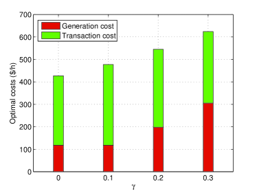
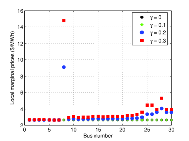
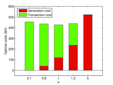
Fig. 1 depicts the optimal costs varying with the regularization weight . It is clear that the conditional transaction cost decreases as increases. Since larger effects heavier penalty on the transaction cost, less will be scheduled to reduce the risk of wind power shortage. This will result in the increase of the conventional generation with the generation cost as shown in Fig. 1.
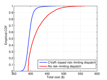
Fig. 2 shows the cumulative distribution functions (CDFs) of the optimal costs of the novel CVaR-based risk-limiting dispatch and no risk-limiting counterpart. For the latter, the forecast wind power quantity is simply used in the nodal balance (12d) for solving (P1), but without the regularizer . Note that after solving (P1) to obtain the optimal dispatch, the generation cost part becomes fixed. Hence, randomness of the total cost comes from that of the transaction cost. Clearly, the no-risk control scheme always incurs a higher total cost than the novel CVaR-based risk-limiting approach. The values of the mean and variance of the optimal total costs are given in Table III, which again speak for the merits of the proposed scheme that exhibits reduced expected cost and variance.
Fig. 3 depicts the optimal power dispatch of conventional generation and committed wind power for both schemes: CVaR-based risk control versus no-risk control. It can be seen that for the CVaR-based approach, the large scheduled wind power at bus makes the lower than that of the no-risk control, and thus gives rise to a lower optimal total cost as corroborated by the CDFs. This happens because the proposed scheme can leverage the condition that purchase price at bus is the lowest one among all wind power injection buses (cf. Table II), which allows for relatively high energy transaction at this bus.
Finally, the effects of demand overload are tested using the results of Figs. 4 and 5. Load demands at all buses are scaled up by , based on the original data of the IEEE -bus system. As expected, the total cost increases with the increase of the overload ratio as confirmed by Fig. 4. It is interesting to observe that the overload hardly affects the transaction cost due to the CVaR-aware risk control mechanism. Being important components of electricity markets, LMPs represent the cost (revenue) of buying (selling) electricity at a particular bus [17]. In Fig. 5, LMPs are plotted for varying overload ratios . Note that all LMPs should be equal in the case of no transmission line congestion. Clearly, the congestion happens as overload demand increases.
V Conclusions and Future Work
CVaR-based DC-OPF with wind integration was investigated in this paper. A convex optimization problem was formulated considering the trade off between conventional generation cost and conditional energy transaction cost. The CVaR-based regularizer plays an important role of risk-limiting dispatch, thus effecting smart utilization of renewables to reduce the cost of conventional power generation, while taking limited risk of wind power shortage.
A number of appealing directions open up towards extending the proposed model and approach. These include CVaR-based UC and AC-OPF, uncertain load demand and transaction costs, as well as distributed scheduling.
Acknowledgement
The authors are grateful to Drs. Vassilis Kekatos and Nikolaos Gatsis for helpful discussions and their aid with the data collection in [6]. The authors also would like to thank Prof. Shuzhong Zhang of the Univ. of Minnesota, for his inspiring suggestion to consider CVaR.
References
- [1] GWEC, “Global wind statistics 2012,” Feb. 2013, [Online]. Available: http://www.gwec.net/wp-content/uploads/2013/02/GWEC-PRstats-2012_english.pdf.
- [2] “20% wind energy by 2030: Increasing wind energy’s contribution to U.S. electricity supply,” July 2008, [Online]. Available: http://www1.eere.energy.gov/wind/pdfs/41869.pdf.
- [3] J. Hetzer, C. Yu, and K. Bhattarai, “An economic dispatch model incorporating wind power,” IEEE Trans. on Energy Conver., vol. 23, no. 2, pp. 603–611, Jun. 2008.
- [4] Y. Zhang, N. Gatsis, and G. B. Giannakis, “Robust energy management for microgrids with high-penetration renewables,” IEEE Trans. on Sustainable Energy, 2013 (to appear).
- [5] ——, “Risk-constrained energy management with multiple wind farms,” in Proc. of Innovative Smart Grid Tech., Washington, D.C., Feb. 2013.
- [6] Y. Zhang, N. Gatsis, V. Kekatos, and G. B. Giannakis, “Risk-aware management of distributed energy resources,” in Proc. of 18th Intl. Conf. on DSP, Santorini Island, Greece, July 2013.
- [7] R. Rajagopal, E. Bitar, F. Wu, and P. Varaiya, “Risk limiting dispatch of wind power,” in Proc. of American Control Conf., Montréal, Canada, June 2012.
- [8] Q. Fang, Y. Guan, and J. Wang, “A chance-constrained two-stage stochastic program for unit commitment with uncertain wind power output,” IEEE Trans. on Power Syst., vol. 27, no. 1, pp. 206–215, 2012.
- [9] D. Bienstock, M. Chertkov, and S. Harnett, “Chance constrained optimal power flow: Risk-aware network control under uncertainty,” Feb. 2013, [Online]. Avaialble: http://arxiv.org/pdf/1209.5779.pdf.
- [10] E. Sjödin, D. F. Gayme, and U. Topcu, “Risk-mitigated optimal power flow for wind powered grids,” in Proc. of American Control Conf., Montréal, Canada, June 2012, pp. 4431–4437.
- [11] Power systems test case archive. Univ. of Washington. [Online]. Available: http://www.ee.washington.edu/research/pstca/
- [12] R. D. Zimmerman, C. E. Murillo-Sánchez, and R. J. Thomas, “MATPOWER: steady-state operations, planning and analysis tools for power systems research and education,” IEEE Trans. on Power Syst., vol. 26, no. 1, pp. 12–19, Feb. 2011.
- [13] Global energy forecasting competition 2012 - wind forecasting. [Online]. Available: http://www.kaggle.com/c/GEF2012-wind-forecasting
- [14] F. J. Fabozzi, P. N. Kolm, D. A. Pachamanova, and S. M. Focardi, Robust Portfolio Optimization and Management. Hoboken, NJ: John Wiley & Sons, 2007.
- [15] R. T. Rockafellar and S. Uryasev, “Optimization of conditional value-at-risk,” Journal of Risk, vol. 2, no. 3, pp. 21–41, 2000.
- [16] ——, “Conditional value-at-risk for general loss distributions,” Journal of Banking and Finance, vol. 26, pp. 1443–1471, 2002.
- [17] A. Gómez-Expósito, A. J. Conejo, and C. Canizares, Eds., Electric Energy Systems, Analysis and Operation. Boca Raton, FL: CRC Press, 2009.
- [18] S. Boyd and L. Vandenberghe, Convex Optimization. Cambridge University Press, 2004.
- [19] R. D. Christie, B. F. Wollenberg, and I. Wangensteen, “Transmission management in the deregulated environment,” Proc. of the IEEE, vol. 88, no. 2, pp. 170–195, Feb. 2000.
- [20] A. J. Kleywegt, A. Shapiro, and T. Homem-De-Mello, “The sample average approximation method for stochastic discrete optimization,” SIAM J. Optim., vol. 12, no. 2, pp. 479–502, 2001.
- [21] CVX Research Inc., “CVX: Matlab software for disciplined convex programming, version 2.0 (beta),” http://cvxr.com/cvx, Sep. 2012.
- [22] J. F. Sturm, “Using SeDuMi 1.02, a MATLAB toolbox for optimization over symmetric cones,” Optim. Meth. Softw., vol. 11–12, pp. 62–653, Aug. 1999.