On the Marčenko–Pastur law for linear time series

Abstract

This paper is concerned with extensions of the classical Marčenko–Pastur law to time series. Specifically, $p$-dimensional linear processes are considered which are built from innovation vectors with independent, identically distributed (real- or complex-valued) entries possessing zero mean, unit variance and finite fourth moments. The coefficient matrices of the linear process are assumed to be simultaneously diagonalizable. In this setting, the limiting behavior of the empirical spectral distribution of both sample covariance and symmetrized sample autocovariance matrices is determined in the high-dimensional setting $p/n\to c\in(0,\infty)$ for which dimension $p$ and sample size $n$ diverge to infinity at the same rate. The results extend existing contributions available in the literature for the covariance case and are one of the first of their kind for the autocovariance case.

FLA

, and T2Supported in part by NSF Grants DMS-12-09226, DMS-13-05858 and DMS-14-07530. T3Supported in part by NSF Grants DMR-10-35468, DMS-11-06690 and DMS-14-07530.

1 Introduction

One of the exciting developments in statistics during the last decade has been the development of the theory and methodologies for dealing with high-dimensional data. The term high dimension is primarily interpreted as meaning that the dimensionality of the observed multivariate data is comparable to the available number of replicates or subjects on which the measurements on the different variables are taken. This is often expressed in the asymptotic framework as $p/n\to c>0$, where $p$ denotes the dimension of the observation vectors (forming a triangular array) and $n$ the sample size. Much of this development centered on understanding the behavior of the sample covariance matrix and especially its eigenvalues and eigenvectors, due to their role in dimension reduction, in estimation of population covariances and as building block of numerous inferential procedures for multivariate data. Comprehensive reviews of this topic can be found in Johnstone j07 and Paul and Aue pa13 .

One most notable high-dimensional phenomena associated with sample covariance matrices is that the sample eigenvalues do not converge to their population counterparts if dimension and sample sizes remain comparable even as the sample size increases. A formal way to express this phenomenon is through the use of the empirical spectral distribution (ESD), that is, the empirical distribution of the eigenvalues of the sample covariance matrix. The celebrated work of Marčenko and Pastur mp67 shows that if one studies a triangular array of random vectors $X_{1},\ldots,X_{n}$, whose components form independent, identically distributed (i.i.d.) random variables with zero mean, unit variance and finite fourth moment, then as $p,n\to\infty$ such that $p/n\to c\in(0,\infty)$, the ESD of $\mathbf{S}=n^{-1}\sum_{j=1}^{n}X_{j}X_{j}^{T}$ converges almost surely to a nonrandom probability distribution known as the Marčenko–Pastur distribution. Since this highly influential discovery a large body of literature under the banner of random matrix theory (RMT) has been developed to explore the properties of the eigenvalues and eigenvectors of large random matrices. One may refer to Anderson et al. agz09 , Bai and Silverstein bs10 and Tao t12 to study various aspects of this literature.

Many important classes of high-dimensional data, particularly those arising in signal processing, economics and finance, have the feature that in addition to the dimensional correlation, the observations are correlated in time. Classical models for time series often assume a stationary correlation structure and use spectral analysis methods or methods built on the behavior of the sample autocovariance matrices for inference and prediction purposes. In spite of this, to our knowledge, no work exists that analyzes the behavior of the sample autocovariance matrices of a time series from a random matrix perspective, even though Jin et al. jwbnh14 have dealt recently covered autocovariance matrices in the independent case. A striking observation is that, in the high-dimensional scenario, the distribution of the eigenvalues of the symmetrized sample autocovariance of a given lag order tends to stabilize to a nondegenerate distribution even in the setting where the observations are i.i.d. This raises questions about the applicability of sample autocovariance matrices as diagnostic tools for determining the nature of temporal dependence in high-dimensional settings. Thus a detailed study of the phenomena associated with the behavior of the ESD of the sample autocovariance matrices when the observations have both dimensional and temporal correlation is of importance to gain a better understanding of the ways in which the dimensionality affects the inference for high-dimensional time series.

All the existing work on high-dimensional time series dealing with the limiting behavior of the ESD focuses on the sample covariance matrix of the data when $X_{1},\ldots,X_{n}$ are $p$-dimensional observations recorded in time and $p,n\to\infty$ such that $p/n\to c\in(0,\infty)$. This includes the works of Jin et al. jwml09 , who assume the process $(X_{t}\dvtx t\in\mathbb{Z})$ has i.i.d. rows with each row following a causal ARMA process. Pfaffel and Schlemm ps12 and Yao y12 extend this framework to the setting where the rows are arbitrary i.i.d. stationary processes with short-range dependence. Zhang z06 , Paul and Silverstein ps09 and El Karoui e09 , under slightly different assumptions, consider the limiting behavior of the ESD of the sample covariance when the data matrices are of the form $\mathbf{A}^{1/2}\mathbf{Z}\mathbf{B}^{1/2}$ where $\mathbf{A}$ and $\mathbf{B}$ are positive semidefinite matrices, and $\mathbf{Z}$ has i.i.d. entries with zero mean, unit variance and finite fourth moment. This model is known as the separable covariance model, since the covariance of the data matrix is the Kronecker product of $\mathbf{A}$ and $\mathbf{B}$. If the rows indicate spatial coordinates and columns indicate time instances, then this model implies that spatial (dimensional) and temporal dependencies in the data are independent of each other. The work of this paper is also partly related to the results of Hachem et al. hln05 , who prove the existence of the limiting ESD for sample covariance of data matrices that are rectangular slices from a bistationary Gaussian process on $\mathbb{Z}^{2}$.

In this paper, the focus is on a class of time series known as linear processes [or $\mathrm{MA}(\infty)$ processes]. The assumptions to be imposed in Section 2 imply that, up to an unknown rotation, the coordinates of the linear process, say $(X_{t}\dvtx t\in\mathbb{Z})$, are uncorrelated stationary linear processes with short range dependence. Extending the work of Jin et al. jwbnh14 to the time series case, the goal is to relate the behavior of the ESD of the lag-$\tau$ symmetrized sample autocovariances, defined as $\mathbf{C}_{\tau}=(2n)^{-1}\sum_{t=1}^{n-\tau}(X_{t}X_{t+\tau}^{*}+X_{t+\tau}X_{t}^{*})$, with ^∗ denoting complex conjugation, to that of the spectra of the coefficient matrices of the linear process when $p,n\to\infty$ such that $p/n\to c\in(0,\infty)$. This requires assuming certain stability conditions on the joint distribution of the eigenvalues of the coefficient matrices which are described later. The class of models under study here includes the class of causal autoregressive moving average (ARMA) processes of finite orders satisfying the requirement that the coefficient matrices are simultaneously diagonalizable and the joint empirical distribution of their eigenvalues (when diagonalized in the common orthogonal or unitary basis), converges to a finite-dimensional distribution. The results are expressed in terms of the Stieltjes transform of the ESD of the sample autocovariances. Specifically, it is shown that the ESD of the symmetrized sample autocovariance matrix of any lag order converges to a nonrandom probability distribution on the real line whose Stieltjes transform can be expressed in terms a unique Stieltjes kernel. The definition of the Stieltjes kernel involves integration with respect to the limiting joint empirical distribution of the eigenvalues of the coefficient matrices as well as the spectral density functions of the one-dimensional processes that correspond to the coordinates of the process $(X_{t}\dvtx t\in\mathbb{Z})$, after rotation in the common unitary or orthogonal matrix that simultaneously diagonalizes the coefficient matrices. Thus this result neatly ties the dimensional correlation, captured by the eigenvalues of the coefficient matrices, with the temporal correlation, captured by the spectral density of the coordinate processes.

The main contributions of this paper are the following: (i) A framework is provided for analyzing the behavior of symmetrized autocovariance matrices of linear processes; (ii) for linear processes satisfying appropriate regularity conditions, a concrete description of the limiting Stieltjes transform is given in terms of the limiting joint ESD of the coefficient matrices and the spectral density of the coordinate processes after a rotation of the coordinates of the observation. Extensions to these main results are (iii) the characterization of the behavior of the ESD of autocovariances of linear filters applied to the observed process; (iv) the description of the ESDs of a class of tapered estimates of the spectral density operator of the observed process that can be used to analyze the long-run variance and spectral coherence of the process. These contributions surpass the work in the existing literature dealing with high-dimensionality effects for time series in two different ways. First, the class of time series models that are analyzed in detail encompasses the setting of stationary i.i.d. rows studied by Jin et al. jwml09 , Pfaffel and Schlemm ps12 and Yao y12 , as well as the setting of separable covariance structure studied by Zhang z06 , Paul and Silverstein ps09 and El Karoui e09 . The proofs of the main results also require more involved arguments. They are partly related to the constructions in Hachem et al. hln05 , but additional technical arguments are needed to go beyond Gaussanity. The results are also related to the work of Hachem et al. hln07 , who studies limiting spectral distributions of covariance matrices for data with a given variance profile. The connection is through the fact that after an approximation of lag operators by circulant shift matrices, and appropriate row and column rotations, the data matrix in our setting can be equivalently expressed as a matrix with independent entries and with a variance profile related to the spectral densities of the different coordinates of the time series. Second, the framework allows for a unified analysis of the ESD of symmetrized autocovariance matrices of all lag orders as well as that of the tapered spectral density operator. None of the existing works deals with the behavior of autocovariances for time series (note again that Jin et al. jwbnh14 treat the i.i.d. case), and this analysis requires a nontrivial variation of the arguments used for dealing with the Stieltjes transform of the sample covariance matrix. Moreover, even though we stick to the setting where the coefficient matrices are Hermitian and simultaneously diagonalizable, the main steps in the derivation, especially the construction of a “deterministic equivalent” of the resolvent of the symmetrized autocovariance matrix, is very general and can be applied to linear processes with structures that go beyond the settings studied in this paper, for example, when the simultaneous diagonalizability of the coefficient matrices is replaced by a form of simultaneous block diagonalizability, even though the latter is not pursued in this paper due to lack of clear statistical motivation. The existence and uniqueness of the limits of the resulting equations and their solutions is the key to establishing the existence of liming ESDs of the autocovariances. This step requires certain regularity conditions on the coefficient matrices and is not pursued beyond the setting described in Section 2. A number of potential applications, for example, to problems in signal processing, and dynamic and static factor models, are discussed in Section 3.

The remaining sections of the paper are organized as follows. Extensions of the main results in Section 2 are discussed in Section 4. The outcomes of a small simulation study are reported in Section 5, while the proofs of the main results are provided in Sections 6–11. Several technical lemmas are collected in the online Supplemental Material (SM) lap-sm .

2 Main results

Let $\mathbb{Z}$ denote the set of integers. A sequence of random vectors $(X_{t}\dvtx t\in\mathbb{Z})$ with values in $\mathbb{C}^{p}$ is called a linear process or moving average process of order infinity, abbreviated by the acronym MA($\infty$), if it has the representation

$$X_{t}=\sum_{\ell=0}^{\infty}\mathbf{A}_{\ell}Z_{t-\ell},\qquad t\in\mathbb{Z},$$ (1)

where $(Z_{t}\dvtx t\in\mathbb{Z})$ denotes a sequence of independent, identically distributed $p$-dimensional random vectors whose entries are independent and satisfy $\mathbb{E}[Z_{jt}]=0$, $\mathbb{E}[|Z_{jt}|^{2}]=1$ and $\mathbb{E}[|Z_{jt}|^{4}]<\infty$, where $Z_{jt}$ denotes the $j$th coordinate of $Z_{t}$. In the complex-valued case this is meant as $\mathbb{E}[\operatorname{Re}(Z_{jt})^{2}]=\mathbb{E}[\operatorname{Im}(Z_{jt})^{2}]=1/2$. It is also assumed that real and imaginary parts are independent. Let further $\mathbf{A}_{0}=\mathbf{I}$, the identity matrix. To ensure finite fourth moments for $(X_{t}\dvtx t\in\mathbb{Z})$ and a sufficiently fast decaying weak dependence structure, Assumption 2.1 below lists several additional conditions imposed on the coefficient matrices $\mathbf{A}_{\ell}$.

The results presented in this paper are concerned with the behavior of the symmetrized lag-$\tau$ sample autocovariances

$$\mathbf{C}_{\tau}=\frac{1}{2n}\sum_{t=1}^{n-\tau}\bigl{(}X_{t}X_{t+\tau}^{*}+X_{t+\tau}X_{t}^{*}\bigr{)},\qquad\tau\in\mathbb{N}_{0},$$

assuming observations for $X_{1},\ldots,X_{n}$ are available. For $\tau=0$, this definition gives the covariance matrix $\mathbf{S}=\mathbf{C}_{0}$ discussed in the Introduction. Note that in order to make predictions in the linear process setting, it is imperative to understand the second-order dynamics which are captured in the population autocovariance matrices $\bolds{\Gamma}_{\tau}=\mathbb{E}[X_{t+\tau}X_{t}^{*}]$, $\tau\in\mathbb{N}_{0}$, as all of the popular prediction algorithms such as the Durbin–Levinson and innovations algorithms are starting from there; see, for example, Lütkepohl l06 . The set-up in (1) provides a (strictly) stationary process and consequently the definition of $\bolds{\Gamma}_{\tau}$ does not depend on the value of $t$. The main goal of this paper is to analyze the behavior of the matrices $\mathbf{C}_{\tau}$, which can be viewed as a special sample counterpart to the corresponding $\bolds{\Gamma}_{\tau}$, in the high-dimensional setting for which $p=p(n)$ is a function of the sample size such that

$$\lim_{n\to\infty}\frac{p}{n}=c\in(0,\infty),$$ (2)

thereby extending the above mentioned Marčenko–Pastur-type results to more general time series models and to autocovariance matrices. We can weaken requirement (2) to “$p/n$ bounded away from zero and infinity,” in which case, the asymptotic results hold for subsequences $(p_{k},n_{k})$ satisfying $p_{k}/n_{k}$ converging to a positive constant $c_{k}$, provided that the structural assumptions on the model continue to hold. Let then $\hat{F}_{\tau}$ denote the empirical spectral distribution (ESD) of $\mathbf{C}_{\tau}$ given by

$$\hat{F}_{\tau}(\sigma)=\frac{1}{p}\sum_{j=1}^{p}\mathbb{I}_{\{\sigma_{j}\leq\sigma\}},$$

where $\sigma_{1},\ldots,\sigma_{p}$ are the eigenvalues of $\mathbf{C}_{\tau}$. The proof techniques for establishing large-sample results about $\hat{F}_{\tau}$ are based on exploiting convergence properties of Stieltjes transforms, which continue to play an important role in verifying theoretical results in RMT; see, for example, Paul and Aue pa13 for a recent summary. The Stieltjes transform of a distribution function $F$ on the real line is the function

$$s_{F}\dvtx\mathbb{C}^{+}\to\mathbb{C}^{+},\qquad z\mapsto s_{F}(z)=\int\frac{1}{\sigma-z}\,dF(\sigma),$$

where $\mathbb{C}^{+}=\{x+iy\dvtx x\in\mathbb{R},y>0\}$ denotes the upper complex half plane. It can be shown that $s_{F}$ is analytic on $\mathbb{C}^{+}$ and that the distribution function $F$ can be reconstructed from $s_{F}$ using an inversion formula; see pa13 . In order to make statements about $\hat{F}_{\tau}$, the following additional assumptions on the coefficient matrices $\mathbf{A}_{\ell}$ are needed. Let $\mathbb{N}$ and $\mathbb{N}_{0}$ denote the positive and nonnegative integers, respectively.

Assumption 2.1.

(a) The matrices $(\mathbf{A}_{\ell}\dvtx\ell\in\mathbb{N}_{0})$ are simultaneously diagonalizable random Hermitian matrices, independent of $(Z_{t}\dvtx t\in\mathbb{Z})$ and satisfying $\|\mathbf{A}_{\ell}\|\leq\bar{\lambda}_{\mathbf{A}_{\ell}}$ for all $\ell\in\mathbb{N}_{0}$ and large $p$ with

$$\sum_{\ell=0}^{\infty}\bar{\lambda}_{\mathbf{A}_{\ell}}\leq\bar{\lambda}_{\mathbf{A}}<\infty\quad\mbox{and}\quad\sum_{\ell=0}^{\infty}\ell\bar{\lambda}_{\mathbf{A}_{\ell}}\leq\bar{\lambda}_{\mathbf{A}}^{\prime}<\infty.$$

Note that one can set $\bar{\lambda}_{\mathbf{A}_{0}}=1$.

(b) There are continuous functions $f_{\ell}\dvtx\mathbb{R}^{m}\to\mathbb{R}$, $\ell\in\mathbb{N}_{0}$, such that, for every $p$, there is a set of points $\lambda_{1},\ldots,\lambda_{p}\in\mathbb{R}^{m}$, not necessarily distinct, and a unitary $p\times p$ matrix $\mathbf{U}$ such that

$$\mathbf{U}^{*}\mathbf{A}_{\ell}\mathbf{U}=\operatorname{diag}\bigl{(}f_{\ell}(\lambda_{1}),\ldots,f_{\ell}(\lambda_{p})\bigr{)},\qquad\ell\in\mathbb{N},$$

and $f_{0}(\lambda)=1$. [Note that the functions $f_{\ell}$ are allowed to depend on $p=p(n)$ as long as they converge to continuous functions as $n\to\infty$ uniformly.]

(c) With probability one, $F_{p}^{\mathbf{A}}$, the ESD of $\{\lambda_{1},\ldots,\lambda_{p}\}$, converges weakly to a nonrandom probability distribution function $F^{\mathbf{A}}$ on $\mathbb{R}^{m}$ as $p\to\infty$.

Let $\mathbf{A}=[\mathbf{A}_{0}\dvtx\mathbf{A}_{1}\dvtx\cdots]$ denote the matrix collecting the coefficient matrices of the linear process $(X_{t}\dvtx t\in\mathbb{Z})$. Define the transfer functions

$$\psi(\lambda,\nu)=\sum_{\ell=0}^{\infty}e^{i\ell\nu}f_{\ell}(\lambda)\quad\mbox{and}\quad\psi(\mathbf{A},\nu)=\sum_{\ell=0}^{\infty}e^{i\ell\nu}\mathbf{A}_{\ell},$$ (3)

as well as the power transfer functions

$$h(\lambda,\nu)=\bigl{|}\psi(\lambda,\nu)\bigr{|}^{2}\quad\mbox{and}\quad\mathcal{H}(\mathbf{A},\nu)=\psi(\mathbf{A},\nu)\psi(\mathbf{A},\nu)^{*}.$$

Note that the contribution of the temporal dependence of the underlying time series on the asymptotic behavior of $\hat{F}_{\tau}$ is quantified through $h(\lambda,\nu)$. Specifically, $h(\lambda_{j},\nu)$ with $\lambda_{j}$ as in part (b) of Assumption 2.1 is (up to normalization) the spectral density of the $j$th coordinate of the process rotated with the help of the unitary matrix $\mathbf{U}$. With these definitions, the main results of this paper can be stated as follows.

Theorem 2.1

If a complex-valued linear process $(X_{t}\dvtx t\in\mathbb{Z})$ with independent, identically distributed $Z_{jt}$, $\mathbb{E}[Z_{jt}]=0$, $\mathbb{E}[\operatorname{Re}(Z_{jt})^{2}]=\mathbb{E}[\operatorname{Im}(Z_{jt})^{2}]=1/2$, $\operatorname{Re}(Z_{jt})$ and $\operatorname{Im}(Z_{jt})$ are independent, and $\mathbb{E}[|Z_{jt}|^{4}]<\infty$, satisfies Assumption 2.1, then, with probability one and in the high-dimensional setting (2), $\hat{F}_{\tau}$ converges to a nonrandom probability distribution $F_{\tau}$ with Stieltjes transform $s_{\tau}$ determined by the equation

$$s_{\tau}(z)=\int\biggl{[}\frac{1}{2\pi}\int_{0}^{2\pi}\frac{\cos(\tau\nu)h(\lambda,\nu)}{1+c\cos(\tau\nu)K_{\tau}(z,\nu)}\,d\nu-z\biggr{]}^{-1}\,dF^{\mathbf{A}}(\lambda),$$ (4)

where $K_{\tau}\dvtx\mathbb{C}^{+}\times[0,2\pi]\to\mathbb{C}^{+}$ is a Stieltjes kernel; that is, $K_{\tau}(\cdot,\nu)$ is the Stieltjes transform of a measure with total mass $m_{\nu}=\int h(\lambda,\nu)\,dF^{\mathbf{A}}(\lambda)$ for every fixed $\nu\in[0,2\pi]$, whenever $m_{\nu}>0$. Moreover, $K_{\tau}$ is the unique solution of

$$K_{\tau}(z,\nu)$$

(5)

$$\qquad=\int\biggl{[}\frac{1}{2\pi}\int_{0}^{2\pi}\frac{\cos(\tau\nu^{\prime})h(\lambda,\nu^{\prime})}{1+c\cos(\tau\nu^{\prime})K_{\tau}(z,\nu^{\prime})}\,d\nu^{\prime}-z\biggr{]}^{-1}h(\lambda,\nu)\,dF^{\mathbf{A}}(\lambda),$$

subject to the restriction that $K_{\tau}$ is a Stieltjes kernel. Otherwise, if $m_{\nu}=0$, then $K_{\tau}(z,\nu)$ is identically zero on $\mathbb{C}^{+}$ and so still satisfies (2.1).

Theorem 2.2

If a real-valued linear process $(X_{t}\dvtx t\in\mathbb{Z})$ with independent, identically distributed real-valued $Z_{jt}$, $\mathbb{E}[Z_{jt}]=0$, $\mathbb{E}[Z_{jt}^{2}]=1$ and $\mathbb{E}[Z_{jt}^{4}]<\infty$, satisfies Assumption 2.1 with real symmetric coefficient matrices $(\mathbf{A}_{\ell}\dvtx\ell\in\mathbb{N}_{0})$, then the result of Theorem 2.1 is retained.

Remark 2.1.

When each coefficient matrix $\mathbf{A}_{\ell}$ is a multiple of the identity matrix, that is, $\mathbf{A}_{\ell}=\alpha_{\ell}I_{p}$ where $(\alpha_{\ell}\dvtx\ell\in\mathbb{N})$ is a sequence of real numbers satisfying $\sum_{\ell=1}^{\infty}\ell|\alpha_{\ell}|<\infty$, the result of Theorem 2.1 reduces to the results obtained in Pfaffel and Schlemm ps12 and Yao y12 .

Remark 2.2.

One can relax the assumption of simultaneous diagonalizability of the coefficient matrices of the linear process to certain forms of near-simultaneous diagonalizability, so that the conclusions of Theorem 2.1 continue to hold for linear processes where the MA coefficients are Toeplitz matrices whose entries decay away from the diagonal at an appropriate rate. Specifically, if $\mathbf{A}_{\ell}$ is the Toeplitz matrix with $j$th row equaling $(a_{k-j,\ell}\dvtx 0\leq k<p)$, for the bi-infinite sequence $(a_{k,\ell})$ satisfying the condition

$$\sum_{\ell=0}^{\infty}\sum_{k=-\infty}^{\infty}|k|^{\beta}(\ell+1)|a_{k,\ell}|<\infty$$

for some $\beta>0$, which in particular implies Assumption 2.1(a) by the Gershgorin theorem, then the existence of the limiting ESD of symmetrized autocovariance matrices can be proved. For brevity, instead of giving a thorough technical argument, we only provide the main idea of proof. First, the $\mathrm{MA}(\infty)$ series is approximated by an $\mathrm{MA}(q_{p})$ series with $q_{p}=O(p^{1/3})$, using arguments along the line of Section 6.3. Second, banding with bandwidth $k_{p}$ is applied to the coefficient matrices $\mathbf{A}_{\ell}$. It can be shown through an application of norm inequality, that the limiting spectral behavior is unchanged under the banding so long as $k_{p}\to\infty$ under (2). Third, circulant matrices are constructed from the banded Toeplitz matrices by periodization. The resulting matrices are therefore simultaneously diagonalizable, and the eigenvalues of the $\ell$th approximate coefficient matrix approximate the transfer function of the sequence $(a_{k,\ell}\dvtx k\in\mathbb{Z})$. The limiting spectral behavior is seen to be unchanged after the use of the rank inequality so long as $k_{p}/p\to 0$ under (2). The rest of the derivations follow the arguments in the proof of Theorem 2.1. While this particular result is related to the work of Hachem et al. hln05 , who study the convergence of the empirical distribution of the sample covariance matrix of rectangular slices of bistationary Gaussian random fields, hln05 does not cover the transition to non-Gaussian processes or the spectral behavior of sample autocovariance matrices.

Several extensions of Theorem 2.1 are discussed in Section 4 below. The proof steps needed in order to verify the main result are outlined in Section 6, and the details are in Sections 7–11. The online SM lap-sm contains additional technical lemmas.

3 Examples and applications

3.1 An $\mathrm{ARMA}(1,1)$ example

In this section, let $(X_{t}\dvtx t\in\mathbb{Z})$ be the causal ARMA($1,1$) process given by the stochastic difference equations

$$\Phi(L)X_{t}=\Theta(L)Z_{t},\qquad t\in\mathbb{Z},$$

where $\Phi(L)=I-\Phi_{1}L$ and $\Theta(L)=I+\Theta_{1}L$ are, respectively, the matrix-valued autoregressive and moving average polynomials in the lag operator $L$ for which it is assumed that $\|\Phi_{1}\|\leq\bar{\phi}<1$ and $\|\Theta_{1}\|\leq\bar{\theta}<\infty$. Moreover, $(Z_{t}\dvtx t\in\mathbb{Z})\sim\mathrm{IID}(0,I)$ with entries possessing finite fourth moments. Under these conditions $(X_{t}\dvtx t\in\mathbb{Z})$ admits the MA($\infty$) representation

$$X_{t}=\mathbf{A}(L)Z_{t},\qquad t\in\mathbb{Z},$$

with $\mathbf{A}(L)=\sum_{\ell=0}^{\infty}\mathbf{A}_{\ell}L^{\ell}=\Phi^{-1}(L)\Theta(L)$. Assume now further that $\Phi_{1}$ and $\Theta_{1}$ are simultaneously diagonalizable. Then $\Phi_{1}=\mathbf{U}\bolds{\Lambda}_{\Phi}\mathbf{U}^{*}$ and $\Theta_{1}=\mathbf{U}\bolds{\Lambda}_{\Theta}\mathbf{U}^{*}$, where $\bolds{\Lambda}_{\Phi}=\operatorname{diag}(\phi_{1},\ldots,\phi_{p})$ and $\bolds{\Lambda}_{\Theta}=\operatorname{diag}(\theta_{1},\ldots,\theta_{p})$ such that $\max_{j}|\phi_{j}|\leq\bar{\phi}$ and $\max_{j}|\theta_{j}|\leq\bar{\theta}$. With regard to Assumption 2.1, let $\lambda_{j}=(\phi_{j},\theta_{j})^{\prime}\in\mathbb{R}^{2}$. Part (c) of the assumption then requires almost sure weak convergence of the ESD of $\{\lambda_{1},\ldots,\lambda_{p}\}$ to a nonrandom probability distribution function on $\mathbb{R}^{2}$. Moreover, using that for each coordinate,

$$\frac{1+\theta_{j}L}{1-\phi_{j}L}=(1+\theta_{j}L)\sum_{\ell=0}^{\infty}(\phi_{j}L)^{\ell}=1+(\theta_{j}+\phi_{j})\sum_{\ell=1}^{\infty}\phi_{j}^{\ell-1}L^{\ell},$$

it follows that $\mathbf{A}_{\ell}=\mathbf{U}\operatorname{diag}(f_{\ell}(\lambda_{1}),\ldots,f_{\ell}(\lambda_{p}))\mathbf{U}^{*}$ with $f_{0}(\lambda_{j})=1$ and $f_{\ell}(\lambda_{j})=(\theta_{j}+\phi_{j})\phi_{j}^{\ell-1}$ for $\ell\in\mathbb{N}$. This illustrates part (b) of Assumption 2.1. The summability conditions stated in part (a) are clearly satisfied. Generalization to arbitrary causal ARMA models follows in a similar fashion.

3.2 Time series with independent rows

In this section, the situation of time series with independent rows is considered. Our results describe the limiting ESD of the symmetrized sample autocovariances in the setting where the $j$th row of the time series, denoted $\{\xi_{jt}\dvtx t\in\mathbb{Z}\}$, is given by

$$\xi_{jt}=\sum_{\ell=0}^{\infty}f_{\ell}(\lambda_{j})Z_{j,t-\ell},$$ (6)

where: (i) the $Z_{jt}$’s are independent, identically distributed real- or complex-valued random variables with mean zero, unit variance and finite fourth moments; (ii) the $f_{\ell}$’s are continuous functions from $\mathbb{R}^{m}\to\mathbb{R}$ satisfying $f_{0}(\lambda)\equiv 1$ and the summability condition $\sup_{\lambda\in\operatorname{supp}(F^{\mathbf{A}})}\sum_{\ell=0}^{\infty}(\ell+1)|f_{\ell}(\lambda)|<\infty$; (iii) the $\lambda_{j}$’s are i.i.d. realizations from an $m$-dimensional probability distribution denoted by $F^{\mathbf{A}}$. If the supremum in condition (ii) is taken over $\mathbb{R}^{m}$, condition (iii) can be weakened to require that the empirical distribution of the $\lambda_{j}$’s converges almost surely to a nonrandom distribution $F^{\mathbf{A}}$.

Let $h(\lambda,\nu)=|\sum_{\ell=0}^{\infty}e^{i\ell\nu}f_{\ell}(\lambda)|^{2}$. Then the empirical distributions of the eigenvalues of the lag-$\tau$ symmetrized autocovariance matrices converge almost surely to a nonrandom probability distribution $F_{\tau}$ with Stieltjes transform $s_{\tau}$ determined by equations (4) and (2.1), where $K_{\tau}(z,\nu)$ is as in Theorem 2.1. This is in the spirit of the works of Jin et al. jwml09 , Pfaffel and Schlemm ps12 and Yao y12 , who studied the sample covariance case with $f_{\ell}(\lambda)\equiv\bar{f}_{\ell}$ for all $\ell\geq 0$, Hachem et al. hln05 , who considered the sample covariance case for stationary Gaussian fields and Jin et al. jwbnh14 , who studied the symmetrized sample autocovariance case with $f_{1}(\lambda)\equiv 1$ and $f_{\ell}(\lambda)\equiv 0$ for $\ell\geq 1$ (i.e., when the $\xi_{jt}$’s are i.i.d. with zero mean and unit variance).

3.3 Signal processing and diagnostic checks

The results derived here can be useful in dealing with a number of important statistical questions. Signal detection in a noisy background is one of the most important problems in signal processing and communications theory. Often the observations are taken in time, and the standard assumption is that the noise is i.i.d. in time, referred to as white noise. However, in spatio-temporal signal processing, it is quite apt to formulate the noise as “colored” or correlated in time, as well as in the spatial dimension. The proposed model for the time series is a good prototype for such a noise structure. Thus the problem of detecting a low-dimensional signal embedded in high-dimensional noise, for example, through a factor model framework, can be effectively addressed by making use of the behavior of the ESDs of autocovariances of the noise. Another potential application of the results is in building diagnostic tools for high-dimensional time series. By focusing on the ESDs of the autocovariances for various lag orders, or that of a tapered estimate of the spectral density operator, one can infer about the nature of dependence, provided the model assumptions hold. The proposed model also provides a broad class of alternatives for the hypothesis of independence of observations in settings where those observations are measured in time. Finally, in practical applications, it is of interest whether the spectrum of the coefficient matrices of the linear process can be estimated from the data. The equations for the limiting Stieltjes kernel and its relation to the Stieltjes transform of the autocovariance matrices provide a tool for attacking this problem. This aspect has been explored in the Ph.D. thesis of the first author l13 and the methodology will be reported elsewhere.

3.4 Dynamic factor models

Forni and Lippi fl99 describe a class of time series models that captures the subject specific variations of microeconomic activities. This class of models, referred to as Dynamic Factor Models (DFM), has proved immensely popular in the econometrics community and beyond. DFMs have, for example, been used for describing the stock returns in ner92 , forecasting national accounts in abr10 , modeling portfolio allocation in aw10 and modeling psychological development in m94 , as well as in many other applications. Important theoretical and inferential questions regarding DFMs have been investigated in a series of papers by Forni and Lippi fl01 , Forni et al. fhlr00 , fhlr04 , fhlr05 and Stock and Watson sw05 , to name a few. DFMs have also shown early promise for applications to other interesting multivariate time series problems such as the study of fMRI data.

A DFM can be described as follows. As in fl99 , let $Y_{jt}$ be the response corresponding to the $j$th individual/agent at time $t$, modeled as

$$Y_{jt}=b_{j1}(L)U_{1t}+\cdots+b_{jM}(L)U_{Mt}+\xi_{jt},\qquad j=1,\ldots,p.$$ (7)

The model specifies that $Y_{jt}$ is determined by a small, fixed number of underlying common factors $U_{kt}$ and their lags, determined by the polynomials $b_{jk}(L)$ in the lag-operator $L$, plus an idiosyncratic component $\xi_{jt}$ assumed independent across individuals. Typically, $(\xi_{jt}\dvtx t\in\mathbb{Z})$ is taken to be a stationary linear processes, independent across $j$.

One of the key questions pertaining to DFM is the determination of the number of dynamic factors. This question has been investigated by Bai and Ng bn07 , Stock and Watson sw05 and Hallin and Liška hl07 . Unlike in PCA, here one has to deal with the additional problem of detecting the lag orders of the dynamic factors. This can be approached through the study of the behavior of the extreme eigenvalues of the sample autocovariance matrices as in Jin et al. jwbnh14 . The issue becomes even more challenging when the dimensionality of the problem increases. In such settings, one expects that a form of phase transition phenomenon, well known in the context of a high-dimensional static factor model (or spiked covariance model) with i.i.d. observations (see, e.g., Baik and Silverstein bs06 ), will set in. In particular, as Jin et al. jwbnh14 argue, a dynamic factor will be detectable from the data only if the corresponding total signal intensity, as measured, for example, by the sum of the variances of the factor loadings, is above a threshold. Moreover, the number of eigenvalues that lie outside the bulk of the eigenvalues of the symmetrized sample autocovariance of a certain lag order provide information about the lag order of the DFM. Driven by the analogy with the static factor model with i.i.d. observations, it is expected that the detection thresholds will depend on the dimension-to-sample size ratio, as well as the behavior of the bulk spectrum of the autocovariances of the idiosyncratic terms at specific lag orders, including the support of the limiting ESD. Equation (6) in Section 3.2 constitutes the “null” model for the DFM in which the dynamic common factors are absent. Therefore follow-up studies on the different aspects of the ESD of the symmetrized sample autocovariances of such processes will be helpful in determining the detection thresholds and estimation characteristics of high-dimensional DFMs.

3.5 An idealized production model

Onatski o12 describes a model for production $Y_{t}$, at time $t$, involving $p$ different industries in an economy that is given by the equations

$$Y_{t}=\mathbf{W}^{-1}\Biggl{(}\sum_{k=1}^{M}u_{kt}\mathbf{f}_{k}+\xi_{t}\Biggr{)}.$$ (8)

Model (8) is a static factor model in which $p\times 1$ vectors $\mathbf{f}_{k}$ denote the (unobserved) common static factors, $u_{kt}$ denote the (unobserved) factor scores consisting of independent time series corresponding to different factors $k$ and $\xi_{t}$ denote the $p\times 1$ vectors of idiosyncratic components. The entries of the matrix $\mathbf{W}$ indicate the interactions among the different industries. In the following an enhanced version of the model is considered where the economy is thought to be divided into a finite number of distinct sectors for which the interaction across the sectors is assumed “weak” in a suitable sense to be described. In addition, the assumption of separable covariance structure of the $\xi_{t}$ made in o12 is relaxed by requiring instead that the temporal variation in $\xi_{t}$ for all the industrial units within a sector is the same and is stationary in time. This assumption means that the component of the vector $\xi_{t}$ corresponding to a particular sector has a separable covariance structure with stationary time variation, and the components corresponding to different sectors are independent. Specifically, if there are $K$ sectors, we can divide $\mathbf{W}$ into $K\times K$ block matrices

$$\mathbf{W}=\left[\matrix{\mathbf{W}_{11}&\mathbf{W}_{12}&\cdots&\mathbf{W}_{1K}\cr\cdot&\cdot&\cdots&\cdot\cr\mathbf{W}_{K1}&\mathbf{W}_{K2}&\cdots&\mathbf{W}_{KK}}\right]=\widetilde{\mathbf{W}}+\Delta,$$

where $\widetilde{\mathbf{W}}=\operatorname{diag}(\mathbf{W}_{11},\ldots,\mathbf{W}_{KK})$. If the sectors have no interaction at all, that is, if $\mathbf{W}_{jk}=0$ for all $j\neq k$, then the corresponding data model is an instance of a blockwise separable covariance model. “Weak interaction” means that the norms of the off-diagonal blocks in the matrix $\mathbf{W}$ are small. More precisely, if $p^{-1}\|\Delta\|_{F}^{2}\to 0$ as $p\to\infty$, then the limiting ESD of the symmetrized autocovariances for the data matrix $\mathbf{Y}$ is the same as that of $\widetilde{\mathbf{Y}}$ obtained by replacing $\mathbf{W}$ by $\widetilde{\mathbf{W}}$ in (8). Under the assumption of a linear process structure on the different components of $\xi_{t}$, and a natural requirement on the stability of the singular values of $\widetilde{\mathbf{W}}$, the existence and characterization of the limiting ESDs of the symmetrized autocovariances of $\widetilde{\mathbf{Y}}$ can be dealt within the framework studied in Section 2. These limiting ESDs will help in determining the detection thresholds for the static factors, or even dynamic factors, if the model were to be enhanced further.

4 Extensions of the main results

This section discusses three different extensions of the main result. The arguments for the proof are similar to that of the proof of Theorem 2.1 and hence only a brief outline is provided. Moreover, the results stated here apply to both real- and complex-valued cases, the only difference being that, in the former case, the relevant matrices are real symmetric while, in the latter case, they are Hermitian.

The first extension involves a rescaling of the process defined in (1). Thus it is assumed that

$$X_{t}=\mathbf{B}^{1/2}\sum_{\ell=0}^{\infty}\mathbf{A}_{\ell}Z_{t-\ell},\qquad t\in\mathbb{Z},$$ (9)

where the processes $(Z_{t}\dvtx t\in\mathbb{Z})$ and matrices $(A_{\ell}\dvtx\ell\in\mathbb{N}_{0})$ satisfy Assumption 2.1, and the matrix $\mathbf{B}^{1/2}$ is the square root of a $p\times p$ positive semidefinite Hermitian (or symmetric) matrix $\mathbf{B}$ satisfying the following assumption.

Assumption 4.1.

Let $\mathbf{U}$ be as in Assumption 2.1. Then

$$\mathbf{U}^{*}\mathbf{B}\mathbf{U}=\operatorname{diag}\bigl{(}g_{\mathbf{B}}(\lambda_{1}),\ldots,g_{\mathbf{B}}(\lambda_{p})\bigr{)},$$

where $g_{\mathbf{B}}\dvtx\mathbb{R}^{m}\to\mathbb{R}_{+}$ is continuous and bounded on $\mathbb{R}^{m}$, and $\{\lambda\dvtx g_{\mathbf{B}}(\lambda)>0\}\cap\operatorname{supp}(F^{\mathbf{A}})$ is nonempty.

As before, $\hat{F}_{\tau}$ is defined to be the ESD of the symmetrized autocovariance $\mathbf{C}_{\tau}$ of lag order $\tau$. If the linear process $(X_{t}\dvtx t\in\mathbb{Z})$ defined through (9) satisfies Assumptions 2.1 and 4.1, then the statement of Theorem 2.1 holds with the function $h(\lambda,\nu)$ replaced by $g_{\mathbf{B}}(\lambda)h(\lambda,\nu)$.

The second extension is about the existence and description of the limiting ESD of the autocovariances of linear filters of the process $(X_{t}\dvtx t\in\mathbb{Z})$ defined through (9). A linear filter of this process is of the form

$$Y_{t}=\sum_{k=0}^{\infty}b_{k}X_{t-k},\qquad t\in\mathbb{Z},$$ (10)

where $(b_{k}\dvtx k\in\mathbb{N}_{0})$ is a sequence of real numbers for which the following summability condition is needed.

Assumption 4.2.

The sequence $(b_{k}\dvtx k\geq 0)$ satisfies $\sum_{k=0}^{\infty}k|b_{k}|<\infty$.

If the linear process $(X_{t}\dvtx t\in\mathbb{Z})$ defined through (9) satisfies Assumptions 2.1 and 4.1, then the statement of Theorem 2.1 holds with the function $h(\lambda,\nu)$ replaced by $\zeta(\nu)g_{\mathbf{B}}(\lambda)h(\lambda,\nu)$, where $\zeta(\nu)=|\sum_{k=0}^{\infty}e^{ik\nu}b_{k}|^{2}$, $\nu\in[0,2\pi]$. This result follows using the properties of convolution and Fourier transform.

The third extension is about estimation of the spectral density operator

$$\Gamma(\eta)=\sum_{\tau=-\infty}^{\infty}e^{i\tau\eta}\mathbb{E}\bigl{[}X_{t}X_{t+\tau}^{*}\bigr{]},\qquad\eta\in[0,2\pi].$$ (11)

It is well known from classical multivariate time series analysis (see, e.g., Chapter 10 of Hamilton h94 ) that the “natural” estimator that replaces the population autocovariance $\mathbb{E}[X_{t}X_{t+\tau}^{*}]$ by the corresponding sample autocovariance may not be positive definite. In order to obtain positive definite estimators and a better bias-variance trade-off, it is therefore standard in the literature to consider certain tapered estimators with standard choices given, for example, by the Bartlett and Parzen kernels as described in h94 . In the following, the behavior of a class of tapered estimators of $\Gamma(\eta)$, which are given by

$$\widehat{\Gamma}_{n}(\eta)=\sum_{\tau=-\infty}^{\infty}T_{n}(\tau)e^{i\tau\eta}\frac{1}{n}\sum_{t=1}^{n-\tau}X_{t}X_{t+\tau}^{*},\qquad\eta\in[0,2\pi],$$ (12)

is studied, where $T_{n}(\cdot)$ is a sequence of even functions and the quantities $T_{n}(\tau)$ are known as tapering weights for which the following restriction is imposed.

Assumption 4.3.

(i) The even functions $T_{n}(\cdot)$ are such that $T_{n}(\tau)=0$ for $\tau\geq n$; (ii) there exists an even function $T(x)$ such that $T_{n}(x)\to T(x)$ as $n\to\infty$ and $|T_{n}(x)|\leq C|T(x)|$ for some $C>0$, for all $x$; (iii) $\sum_{\tau=0}^{\infty}(1+|\tau|)|T(\tau)|<\infty$.

An implication of this assumption is that the function $\mathfrak{f}_{T}(\eta)$ defined by

$$\mathfrak{f}_{T}(\eta)=1+2\sum_{\tau=1}^{\infty}T(\tau)\cos(\tau\eta)$$ (13)

is well defined and is uniformly Lipschitz, and $\mathfrak{f}_{T_{n}}(\eta)=1+\sum_{\tau=1}^{\infty}T_{n}(\tau)\cos(\tau\eta)$ converges to $\mathfrak{f}_{T}(\eta)$ uniformly in $\eta$. Examples of kernels $T_{n}$ are $T_{n}(x)=(1+|x|)^{-\alpha}\mathbb{I}(|x|<n)$ for $\alpha>2$ and $T_{n}(x)=\beta^{|x|}\mathbb{I}(|x|<n)$ for $\beta\in(0,1)$. It can be seen from Assumption 4.3 that in the high-dimensional setting under consideration here, standard choices for tapering weights, such as those given by the Bartlett and Parzen kernels, are ruled out. Now the following generalization of Theorem 2.1 is obtained.

Theorem 4.1

Suppose that the linear process $(X_{t}\dvtx t\in\mathbb{Z})$ defined through (9) satisfies Assumptions 2.1 and 4.1, and that the estimated spectral density operators $(\widehat{\Gamma}_{n}(\eta)\dvtx\eta\in[0,2\pi])$ are defined by (12) with tapering weights satisfying Assumption 4.3. Then, with probability one and in the high-dimensional setting (2), for every $\eta\in[0,2\pi]$, the ESD of $\widehat{\Gamma}_{n}(\eta)$ converges weakly to a probability distribution $F_{T,\eta}$ with Stieltjes transform $s_{T,\eta}$ determined by the equation

$$s_{T,\eta}(z)=\int\biggl{[}\frac{1}{2\pi}\int_{0}^{2\pi}\frac{\mathfrak{f}_{T}(\eta-\nu)g_{\mathbf{B}}(\lambda)h(\lambda,\nu)}{1+c\mathfrak{f}_{T}(\eta-\nu)K_{T,\eta}(z,\nu)}\,d\nu-z\biggr{]}^{-1}\,dF^{\mathbf{A}}(\lambda),$$

where $K_{T,\eta}\dvtx\mathbb{C}^{+}\times[0,2\pi]\to\mathbb{C}^{+}$ is a Stieltjes kernel; that is, $K_{T,\eta}(\cdot,\nu)$ is the Stieltjes transform of a measure with total mass $m_{\nu}=\int g_{\mathbf{B}}(\lambda)h(\lambda,\nu)\,dF^{\mathbf{A}}(\lambda)$ for every fixed $\nu\in[0,2\pi]$, whenever $m_{\nu}>0$. Moreover, $K_{T,\eta}$ is the unique solution to

$$K_{T,\eta}(z,\nu)$$

$$\qquad=\int\biggl{[}\frac{1}{2\pi}\int_{0}^{2\pi}\frac{\mathfrak{f}_{T}(\eta-\nu^{\prime})g_{\mathbf{B}}(\lambda)h(\lambda,\nu^{\prime})}{1+c\mathfrak{f}_{T}(\eta-\nu^{\prime})K_{T,\eta}(z,\nu^{\prime})}\,d\nu^{\prime}-z\biggr{]}^{-1}$$

$$\quad\qquad{}\hskip 7.0pt\times g_{\mathbf{B}}(\lambda)h(\lambda,\nu)\,dF^{\mathbf{A}}(\lambda),$$

subject to the restriction that $K_{T,\eta}$ is a Stieltjes kernel. Else, if $m_{\nu}=0$, $K_{T,\eta}(z,\nu)$ is identically zero on $\mathbb{C}^{+}$ and so still satisfies the latter equation.

Section 6.5 outlines the main argument needed to prove Theorem 4.1.

5 Simulations

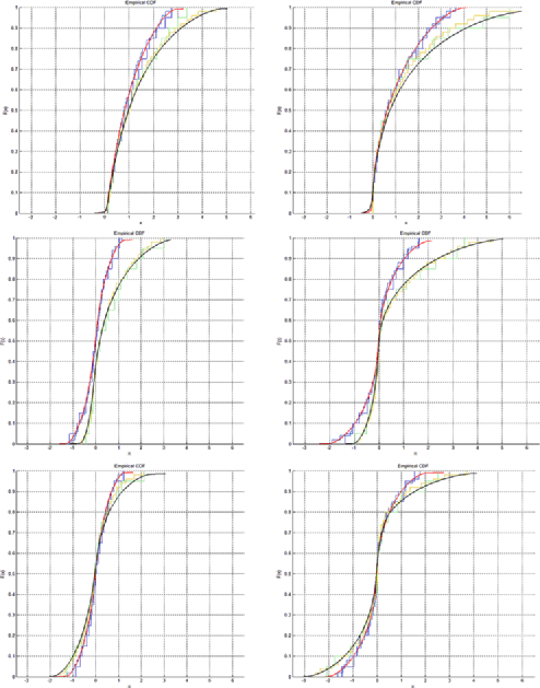
Figure 1: ESDs and LSDs of the sample autocovariances for i.i.d. and $\mathrm{MA}(1)$ observations. Left panel: $p/n=0.5$; right panel: $p/n=1$. Top panel: $\tau=0$; middle panel: $\tau=1$; bottom panel: $\tau=2$. Red curve: LSD for i.i.d.; black curve: LSD for $\mathrm{MA}(1)$. ESDs are corresponding to $p=20$ [deep blue for i.i.d., light green for $\mathrm{MA}(1)$] and $p=50$ [light blue for i.i.d., orange for $\mathrm{MA}(1)$].

In this section, a small simulation study is conducted to illustrate the behavior of the LSD (limiting ESD) of the symmetrized sample autocovariances $\mathbf{C}_{\tau}$ for different lag orders $\tau$ when the observations are i.i.d. ($X_{t}=Z_{t}$) versus when they come from an $\mathrm{MA}(1)$ process ($X_{t}=Z_{t}+\mathbf{A}_{1}Z_{t-1}$) with a symmetric coefficient matrix $\mathbf{A}_{1}$. In this study, two different sets of $(n,p)$ are chosen such that $p/n=0.5$ and $p/n=1$, respectively, for $p=20$ and 50. Also, for the $\mathrm{MA}(1)$ case, the ESD of $\mathbf{A}_{1}$ is chosen to be $0.5\delta_{0.2}+0.5\delta_{0.8}$, where $\delta_{b}$ denotes the degenerate distribution at $b$. The distribution of the $Z_{jt}$’s is chosen to be i.i.d. $N(0,1)$. In Figure 1, the ESD of $\mathbf{C}_{\tau}$ is plotted for the lags $\tau=0,1,2$, for one random realization corresponding to each setting. The theoretical limits (c.d.f.) for all cases are plotted as solid smooth curves [red for i.i.d. and black for $\mathrm{MA}(1)$]. These c.d.f.’s are obtained through numerically inverting the Stieltjes transform $s_{\tau}$ of the LSD of $\mathbf{C}_{\tau}$ using the inversion formula for Stieltjes transforms; cf. bs10 , pa13 . Here $s_{\tau}$ is obtained from equations (4) and (2.1) where $c=p/n$ and $h(\lambda,\nu)=1+2\cos(\nu)\lambda+\lambda^{2}$. Given $F^{\mathbf{A}}=0.5\delta_{0.2}+0.5\delta_{0.8}$, the Stieltjes kernel $K_{\tau}(z,\nu)$ for the $\mathrm{MA}(1)$ case is solved numerically by using calculus of residues. The computational algorithm can be found in the first author’s Ph.D. thesis l13 .

The graphs clearly show the distinction in behavior of ESD of symmetrized sample autocovariances between the i.i.d. and the $\mathrm{MA}(1)$ processes. The LSDs of $\mathbf{C}_{\tau}$ for the i.i.d. case for $\tau=1$ and 2 are the same, which follows immediately from equations (4) and (2.1) that reduce to a single equation since the i.i.d. case corresponds to $F^{\mathbf{A}}=\delta_{0}$. The behavior of the LSDs in the $\mathrm{MA}(1)$ case is distinctly different. It can be shown that LSDs of $\mathbf{C}_{\tau}$ in the $\mathrm{MA}(1)$ case converge to the LSD for $\mathbf{C}_{1}$ in the i.i.d. case as $\tau$ becomes larger. Owing to space constraints, the graphical displays for higher lags are omitted. Another important feature is that the LSDs approximate the ESDs quite well even for $p$ as small as 20, indicating a fast convergence.

6 The structure of the proof

6.1 Developing intuition for the Gaussian $\mathrm{MA}(1)$ case

In this section, the overall proof strategy is briefly outlined, and the intuition behind the individual steps is developed for simpler first-order moving average, $\mathrm{MA}(1)$, time series. The key ideas in the proof of Theorem 2.1 consist of showing that:

• there is a unique Stieltjes kernel solution $K_{\tau}$ to equation (2.1);

• almost surely, the Stieltjes transform of $\hat{F}_{\tau}$, say, $s_{p,\tau}$ converges pointwise to a Stieltjes transform $s_{\tau}$ which will be identified with $F_{\tau}$;

• $\hat{F}_{\tau}$ is tight.

To achieve the second item, one can argue as follows. First, replace the original linear process observations $X_{1},\ldots,X_{n}$ with transformed vectors $\tilde{X}_{1},\ldots,\tilde{X}_{n}$ that are serially independent. Second, replace the symmetrized lag-$\tau$ autocovariance matrix $\mathbf{C}_{\tau}$ by a transformed version $\tilde{\mathbf{C}}_{\tau}$ built from $\tilde{X}_{1},\ldots,\tilde{X}_{n}$. A heuristic formulation for the simpler Gaussian $\mathrm{MA}(1)$ case is given below in some detail. Once these two steps have been achieved, the proof proceeds by verifying some technical conditions with the help of classical RMT results, available, for example, in the monograph Bai and Silverstein bs10 . In the following, let $(X_{t}\dvtx t\in\mathbb{Z})$ denote the $p$-dimensional $\mathrm{MA}(1)$ process given by the equations

$$X_{t}=Z_{t}+\mathbf{A}_{1}Z_{t-1},\qquad t\in\mathbb{Z},$$ (14)

where $(Z_{t}\dvtx t\in\mathbb{Z})$ are assumed complex Gaussian in addition to the requirements of Section 2. For this time series, the conditions imposed through Assumption 2.1 simplify considerably with part (a) reducing to the condition that the eigenvalues of $\mathbf{A}_{1}$ be uniformly bounded and part (b) being satisfied by choosing $f_{1}$ as the identity. Moreover, $\mathbf{A}=[\mathbf{I}\dvtx\mathbf{A}_{1}]$, $\psi(\lambda,\nu)=1+e^{i\nu}\lambda$, $\psi(\mathbf{A},\nu)=\mathbf{I}+e^{i\nu}\mathbf{A}_{1}$, $h(\lambda,\nu)=1+2\cos(\nu)\lambda+\lambda^{2}$ and $\mathcal{H}(\mathbf{A},\nu)=\mathbf{I}+2\cos(\nu)\mathbf{A}_{1}+\mathbf{A}_{1}^{2}$, implying for each $\lambda$, $h(\lambda,\nu)$ is the spectral density (up to normalization) of a univariate $\mathrm{MA}(1)$ process with parameter $\lambda$.

The transformation to serial independence requires two steps, the first consisting of an approximation of the lag operator by a circulant matrix and the second of a rotation using the complex Fourier basis to achieve independence. Accordingly, let

$$\mathbf{L}=[o\dvtx e_{1}\dvtx\cdots\dvtx e_{n-1}]\quad\mbox{and}\quad\tilde{\mathbf{L}}=[e_{n}\dvtx e_{1}\dvtx\cdots\dvtx e_{n-1}]$$

be the $n\times n$ lag operator and its approximating circulant matrix, respectively, where $o$ denotes the $n$-dimensional zero vector and $e_{j}$ the $j$th canonical unit vector in $\mathbb{R}^{n}$ taking the value 1 in the $j$th component and 0 elsewhere. Since $\tilde{\mathbf{L}}$ is a circulant matrix, its spectral decomposition is $\tilde{\mathbf{L}}u_{t}=\eta_{t}u_{t}$, $t=1,\ldots,n$, where $\eta_{t}=e^{i\nu_{t}}$, $\nu_{t}={2\pi t}/{n}$ and $u_{t}$ the vector whose $j$th entry is $\eta_{t}^{j}$. It follows that $\tilde{\mathbf{L}}$ diagonalizes in the complex Fourier basis with the usual Fourier frequencies. Let $\bolds{\Lambda}_{\tilde{\mathbf{L}}}=\operatorname{diag}(\eta_{1},\ldots,\eta_{n})$ and $\mathbf{U}_{\tilde{\mathbf{L}}}=[u_{1}\dvtx\cdots\dvtx u_{n}]$ denote the corresponding eigenvalue and eigenvector matrices, so that $\tilde{\mathbf{L}}=\mathbf{U}_{\tilde{\mathbf{L}}}\bolds{\Lambda}_{\tilde{\mathbf{L}}}\mathbf{U}_{\tilde{\mathbf{L}}}^{*}$. Using $\mathbf{X}=[X_{1}\dvtx\cdots\dvtx X_{n}]$ and $\mathbf{Z}=[Z_{1}\dvtx\cdots\dvtx Z_{n}]$, the $\mathrm{MA}(1)$ process (14) can be transformed into

$$\mathbf{X}_{1}=\mathbf{Z}+\mathbf{A}_{1}\mathbf{Z}\tilde{\mathbf{L}},$$

where $\mathbf{X}_{1}$ constitutes a redefinition of $\mathbf{X}$ such that the first column is changed to $Z_{1}+\mathbf{A}_{1}Z_{n}$, while all other columns are as in the original data matrix $\mathbf{X}$. Rotating in the complex Fourier basis, the observations are transformed again into the vectors $\tilde{X}_{1},\ldots,\tilde{X}_{n}$ given by

$$\tilde{\mathbf{X}}=[\tilde{X}_{1}\dvtx\cdots\dvtx\tilde{X}_{n}]=\mathbf{X}_{1}\mathbf{U}_{\tilde{\mathbf{L}}}.$$

Observe that $\tilde{\mathbf{X}}$ has independent columns. To see this, note first that $\tilde{\mathbf{Z}}=\mathbf{Z}\mathbf{U}_{\tilde{\mathbf{L}}}$ possesses the same distribution as $\mathbf{Z}$, since $\mathbf{Z}$ has (complex) Gaussian entries and $\mathbf{U}_{\tilde{\mathbf{L}}}$ is a unitary matrix. Write then

$$\tilde{\mathbf{X}}=\tilde{\mathbf{Z}}+\mathbf{A}_{1}\tilde{\mathbf{Z}}\bolds{\Lambda}_{\tilde{\mathbf{L}}}=\bigl{[}(\mathbf{I}+\eta_{1}\mathbf{A}_{1})\tilde{Z}_{1}\dvtx\cdots\dvtx(\mathbf{I}+\eta_{n}\mathbf{A}_{1})\tilde{Z}_{n}\bigr{]},$$

where $\tilde{\mathbf{Z}}=[\tilde{Z}_{1}\dvtx\cdots\dvtx\tilde{Z}_{n}]$, and independence of the columns (and thus serial independence) follows. Note also that $\mathbf{I}+\eta_{t}\mathbf{A}_{1}=\psi(\mathbf{A},\nu_{t})$ and consequently $\tilde{\mathbf{X}}=\psi(\mathbf{A},\nu_{t})\tilde{\mathbf{Z}}$, using the transfer function $\psi$ defined in (3).

The vectors $\tilde{X}_{1},\ldots,\tilde{X}_{n}$ give rise to approximations $\tilde{\mathbf{C}}_{\tau}$ to the lag-$\tau$ symmetrized autocovariance matrices $\mathbf{C}_{\tau}$; in particular $\tilde{\mathbf{C}}_{\tau}$ and $\mathbf{C}_{\tau}$ will be shown to have the same large-sample spectral behavior, irrespective of the distribution of the entries. So let

$$\tilde{\mathbf{C}}_{\tau}\equiv\frac{1}{2n}\mathbf{X}_{1}\bigl{(}\tilde{\mathbf{L}}^{\tau}+\bigl{[}\tilde{\mathbf{L}}^{*}\bigr{]}^{\tau}\bigr{)}\mathbf{X}_{1}^{*}=\frac{1}{n}\sum_{t=1}^{n}\cos(\tau\nu_{t})\tilde{X}_{t}\tilde{X}_{t}^{*},$$

where the latter equality follows from several small computations using the quantities introduced in the preceding paragraph. Now,

$$\mathbf{C}_{\tau}-\tilde{\mathbf{C}}_{\tau} = \biggl{(}\mathbf{C}_{\tau}-\frac{1}{2n}\mathbf{X}_{1}\bigl{(}\mathbf{L}^{\tau}+\bigl{[}\mathbf{L}^{*}\bigr{]}^{\tau}\bigr{)}\mathbf{X}_{1}^{*}\biggr{)}$$

$${}+\biggl{(}\frac{1}{2n}\mathbf{X}_{1}\bigl{(}\mathbf{L}^{\tau}+\bigl{[}\mathbf{L}^{*}\bigr{]}^{\tau}\bigr{)}\mathbf{X}_{1}^{*}-\frac{1}{2n}\mathbf{X}_{1}\bigl{(}\tilde{\mathbf{L}}^{\tau}+\bigl{[}\tilde{\mathbf{L}}^{*}\bigr{]}^{\tau}\bigr{)}\mathbf{X}_{1}^{*}\biggr{)}.$$

The rank of the first difference on the right-hand side of the last display is at most $2$, since $\mathbf{X}$ and $\mathbf{X}_{1}$ differ only in the first column. The rank of the second difference is at most $2\tau$. The rank of $\mathbf{C}_{\tau}-\tilde{\mathbf{C}}_{\tau}$ is therefore at most $2(1+\tau)$. Defining the resolvents

$$\mathbf{R}_{\tau}(z)=(\mathbf{C}_{\tau}-z\mathbf{I})^{-1}\quad\mbox{and}\quad\tilde{\mathbf{R}}_{\tau}(z)=(\tilde{\mathbf{C}}_{\tau}-z\mathbf{I})^{-1},$$

the Stieltjes transforms corresponding to the ESDs of $\mathbf{C}_{\tau}$ and $\tilde{\mathbf{C}}_{\tau}$ are, respectively, given by

$$s_{\tau,p}(z)=\frac{1}{p}\operatorname{tr}\bigl{[}\mathbf{R}_{\tau}(z)\bigr{]}\quad\mbox{and}\quad\tilde{s}_{\tau,p}(z)=\frac{1}{p}\operatorname{tr}\bigl{[}\tilde{\mathbf{R}}_{\tau}(z)\bigr{]}.$$

It follows from Lemma S.2 that with probability one, the ESDs of $\mathbf{C}_{\tau}$ and $\tilde{\mathbf{C}}_{\tau}$ converge to the same limit, provided the limits exist. We conclude from Lemma S.3 that the ESD of $\tilde{\mathbf{C}}_{\tau}$ converges a.s. to a nonrandom distribution by showing that $\tilde{s}_{\tau,p}$ converge pointwise a.s. to the Stieltjes transform of a probability measure, thus establishing a.s. convergence of the ESD of $\mathbf{C}_{\tau}$.

In order to derive limiting equation (2.1), a finite sample counterpart is needed. This can be derived as follows. The transformed data $\tilde{\mathbf{X}}$ gives rise to the transformed Stieltjes kernel $\tilde{K}_{\tau}\dvtx\mathbb{C}^{+}\times[0,2\pi]\to\mathbb{C}^{+}$ given by

$$\tilde{K}_{\tau}(z,\nu)=\frac{1}{p}\operatorname{tr}\bigl{[}\tilde{\mathbf{R}}_{\tau}(z)\mathcal{H}(\mathbf{A},\nu)\bigr{]}.$$

Following arguments typically used to establish the deterministic equivalent of a resolvent matrix, $p\times p$ matrix-valued function solutions $(\mathbf{H}_{\tau,p}(z)\dvtx p\in\mathbb{N})$ are needed such that, for sufficiently large $p$,

$$\frac{1}{p}\operatorname{tr}\bigl{[}\bigl{(}\bigl{(}\mathbf{I}+\mathbf{H}_{\tau,p}(z)\bigr{)}^{-1}+z\tilde{\mathbf{R}}_{\tau}(z)\bigr{)}\mathbf{D}_{p}\bigr{]}\approx 0$$ (15)

for all $z\in\mathbb{C}^{+}$ and all $p\times p$ Hermitian matrix sequences $(\mathbf{D}_{p}\dvtx p\in\mathbb{N})$ with uniformly bounded norms $\|\mathbf{D}_{p}\|$. If one uses $\mathbf{D}_{p}=\mathcal{H}(\mathbf{A},\nu)$ and the definition of $\tilde{K}_{\tau}$, the latter approximate equation becomes

$$\tilde{K}_{\tau}(z,\nu)\approx-\frac{1}{pz}\operatorname{tr}\bigl{[}\bigl{(}\mathbf{I}+\mathbf{H}_{\tau,p}(z)\bigr{)}^{-1}\mathcal{H}(\mathbf{A},\nu)\bigr{]}.$$

Section 7 below is devoted to making precise the use of $\approx$ in the above equations and to showing that choosing

$$\mathbf{H}_{\tau,p}(z)=-\frac{1}{zn}\sum_{t=1}^{n}\frac{\cos(\tau\nu_{t})\mathcal{H}(\mathbf{A},\nu_{t})}{1+c_{n}\cos(\tau\nu_{t})\tilde{K}_{\tau}(z,\nu_{t})},$$ (16)

with $\nu_{t}=2\pi t/n$ and $c_{n}=p/n$, is appropriate.

6.2 Extension to the non-Gaussian case

In order to verify the statement of Theorem 2.1 for non-Gaussian innovations $(Z_{t}\dvtx t\in\mathbb{Z})$, two key ideas are invoked, namely showing that:

• for any $z\in\mathbb{C}^{+}$, the Stieltjes transform $s_{p}(z)$ concentrates around $\mathbb{E}[s_{p}(z)]$ regardless of the underlying distributional assumption;

• the difference between the expectations $\mathbb{E}[s_{p}(z)]$ under the Gaussian model and the non-Gaussian model is asymptotically negligible.

To establish the concentration property of the first item, McDiarmid’s inequality is used to bound probabilities of the type $\mathbb{P}(|s_{p}(z)-\mathbb{E}[s_{p}(z)]|\geq\varepsilon)$ for arbitrary $\varepsilon>0$. These probabilities are then shown to converge to zero exponentially fast under (2). To establish the second item, the generalized Lindeberg principle of Chatterjee c06 is applied. To this end, the argument $z$ is viewed as a parameter and $s_{p}(z)$ as a function of the real parts $Z_{jt}^{R}$ and the imaginary parts $Z_{jt}^{I}$ of the innovation entries $Z_{jt}$, for $j=1,\ldots,p$ and $t=1,\ldots,n$. The difference between Gaussian $Z_{t}$ and non-Gaussian $Z_{t}$ can then be analyzed by consecutively changing one pair $(Z_{jt}^{R},Z_{jt}^{I})$ from Gaussian to non-Gaussian, thereby expressing the respective differences in the expected Stieltjes transforms as a sum of these entrywise changes. These differences will be evaluated through a Taylor series expansion, bounding certain third-order partial derivatives of $s_{p}$. Details are given in Section 9.

6.3 Extension to the linear process case

While the arguments established so far work in the same fashion also for MA($q$) processes, certain difficulties arise when making the transition to the MA($\infty$) or linear process case. First, if one constructs the data matrix $\mathbf{X}$ not from $\mathrm{MA}(1)$ observations as above but from the linear process $X_{t}=\sum_{\ell=0}^{\infty}\mathbf{A}_{\ell}Z_{t-\ell}$, then every column of $\mathbf{X}$ is different from the corresponding column in the transformed matrix $\mathbf{X}_{\infty}=\sum_{\ell=0}^{\infty}\mathbf{A}_{\ell}\mathbf{Z}\tilde{\mathbf{L}}^{\ell}$ and not only the first column [or the first $q$ columns for the MA($q$) case]. Second, for the $\mathrm{MA}(1)$ case one can write the Stieltjes transform $s_{p}(z)$ as a function of $2p(n+1)$ variables $Z_{jt}^{R}$ and $Z_{jt}^{I}$ [or $2p(n+q)$ variables for the MA($q$) case], but for linear processes, even for finite $p$, $s_{p}(z)$ is a function of infinitely many $Z_{jt}^{R}$ and $Z_{jt}^{I}$. This makes their study substantially harder.

Linear processes are thus, for the purposes of this paper, approached through truncation, that is, by approximation through finite-order MA processes $X_{t}=\sum_{\ell=0}^{q(p)}\mathbf{A}_{\ell}Z_{t-\ell}$ whose order $q(p)$ is a function of the dimension $p$ and therefore grows with the sample size under (2). Obviously $q(p)\to\infty$ is a necessary condition to make this approximation work. However, $q(p)$ cannot grow too fast (leading to the same difficulties in transitioning from the Gaussian to the non-Gaussian case as for the linear process itself) or too slow (showing that the LSDs of the linear process and its truncated version are identical becomes an issue). It turns out in Section 10 that $q(p)=\lceil p^{1/3}\rceil$, with $\lceil\cdot\rceil$ denoting the ceiling function, is an appropriate choice.

6.4 Including the real-valued case

To address the statements of Theorem 2.2, the arguments presented thus far have to be adjusted for real-valued innovations $(Z_{t}\dvtx t\in\mathbb{Z})$. This is done using the eigen-decomposition of the coefficient matrices in the real Fourier basis, after which arguments already developed for the complex case apply. Detailed steps are given in Section 11.

6.5 Dealing with the spectral density operator

The key step toward proving Theorem 4.1 is to express $\widehat{\Gamma}_{n}(\eta)$ as

$$\widehat{\Gamma}_{n}(\eta) = \sum_{\tau=-\infty}^{\infty}T_{n}(\tau)e^{i\tau\eta}\frac{1}{n}\mathbf{X}\mathbf{L}^{-\tau}\mathbf{X}^{*}$$

$$= \frac{1}{n}\mathbf{X}\Biggl{(}\mathbf{I}_{p}+\sum_{\tau=1}^{\infty}T_{n}(\tau)\bigl{(}e^{i\tau\eta}\mathbf{L}^{-\tau}+e^{-i\tau\eta}\mathbf{L}^{\tau}\bigr{)}\Biggr{)}\mathbf{X}^{*},$$

and then noticing that the matrix $\mathbf{I}_{p}+\sum_{\tau=1}^{\infty}T_{n}(\tau)(e^{i\tau\eta}\tilde{\mathbf{L}}^{\tau}+e^{-i\tau\eta}\tilde{\mathbf{L}}^{-\tau})$ diagonalizes in the (real or complex) Fourier basis with eigenvalues $\mathfrak{f}_{T_{n}}(\eta-\nu_{t})$, for $t=1,\ldots,n$, so that the ESD of $\widehat{\Gamma}_{n}(\eta)$ can be approximated by the ESD of the matrix $\widetilde{\Gamma}_{n}(\eta)=n^{-1}\sum_{t=1}^{n}\mathfrak{f}_{T_{n}}(\eta-\nu_{t})\tilde{X}_{t}\tilde{X}_{t}^{*}$, where $\tilde{X}_{t}^{*}$ is the $t$th column of the matrix $\mathbf{X}\mathbf{F}_{n}^{*}$, and $\mathbf{F}_{n}$ denotes the $n\times n$ Fourier rotation matrix. We give the main steps of the arguments leading to this result. First, suppose that $m_{n}\to\infty$ such that $m_{n}/n\to 0$ as $n\to\infty$. Then we can write

$$\widehat{\Gamma}_{n}(\eta)=\widetilde{\Gamma}_{n,m_{n}}^{(1)}(\eta)+\bigl{(}\widehat{\Gamma}_{n,m_{n}}^{(1)}(\eta)-\widetilde{\Gamma}_{n,m_{n}}^{(1)}(\eta)\bigr{)}+\widehat{\Gamma}_{n,m_{n}}^{(2)}(\eta),$$ (17)

where

$$\widetilde{\Gamma}_{n,m_{n}}^{(1)}(\eta) = \frac{1}{n}\mathbf{X}\Biggl{(}\mathbf{I}_{p}+\sum_{\tau=1}^{m_{n}}T_{n}(\tau)\bigl{(}e^{i\tau\eta}\tilde{\mathbf{L}}^{-\tau}+e^{-i\tau\eta}\tilde{\mathbf{L}}^{\tau}\bigr{)}\Biggr{)}\mathbf{X}^{*}$$

$$= \frac{1}{n}\sum_{t=1}^{n}\mathfrak{f}_{T_{n},m_{n}}(\eta-\nu_{t})\tilde{X}_{t}\tilde{X}_{t}^{*},$$

with $\mathfrak{f}_{T_{n},m_{n}}(\theta)=1+2\sum_{\tau=1}^{m_{n}}\cos(\tau\theta)$,

$$\widehat{\Gamma}_{n,m_{n}}^{(1)}(\eta)=\frac{1}{n}\mathbf{X}\Biggl{(}\mathbf{I}_{p}+\sum_{\tau=1}^{m_{n}}T_{n}(\tau)\bigl{(}e^{i\tau\eta}\mathbf{L}^{-\tau}+e^{-i\tau\eta}\mathbf{L}^{\tau}\bigr{)}\Biggr{)}\mathbf{X}^{*}$$

and

$$\widehat{\Gamma}_{n,m_{n}}^{(2)}(\eta)=\frac{1}{n}\mathbf{X}\Biggl{(}\sum_{\tau=m_{n}+1}^{n}T_{n}(\tau)\bigl{(}e^{i\tau\eta}\mathbf{L}^{-\tau}+e^{-i\tau\eta}\mathbf{L}^{\tau}\bigr{)}\Biggr{)}\mathbf{X}^{*}.$$

Now, the following facts together with representation (17) and Theorem A.43 of Bai and Silverstein bs10 (rank inequality) and Lemma S.1 (norm inequality) prove the assertion: [(iii)]

$\sup_{\theta\in[0,2\pi]}\max\{|\mathfrak{f}_{T_{n},m_{n}}(\theta)-\mathfrak{f}_{T_{n}}(\theta)|,|\mathfrak{f}_{T_{n}}(\theta)-\mathfrak{f}_{T}(\theta)|\}\to 0$, as $n\to\infty$;

rank$(\widehat{\Gamma}_{n,m_{n}}^{(1)}(\eta)-\widetilde{\Gamma}_{n,m_{n}}^{(1)}(\eta))\leq 2m_{n}=o(p)$;

$$p^{-1}\bigl{\|}\widehat{\Gamma}_{n,m_{n}}^{(2)}(\eta)\bigr{\|}_{F}^{2}\leq\bigl{\|}\widehat{\Gamma}_{n,m_{n}}^{(2)}(\eta)\bigr{\|}^{2}$$

and

$$\big{\|}\widehat{\Gamma}_{n,m_{n}}^{(2)}(\eta)\big{\|}\leq\big{\|}n^{-1}\mathbf{X}\mathbf{X}^{*}\big{\|}\sum_{\tau=m_{n}+1}^{\infty}\big{|}T_{n}(\tau)\big{|}\to 0\qquad\mbox{a.s.}$$

7 Proof for the complex Gaussian $\mathrm{MA}(q)$ case

Throughout, $(\mathbf{A}_{\ell}\dvtx\ell\in\mathbb{N})$ is treated as a sequence of nonrandom matrices, and all the arguments are valid conditionally on this sequence. In this section, the result of Theorem 2.1 is first verified for the MA($q$) process $X_{t}=\sum_{\ell=0}^{q}\mathbf{A}_{\ell}Z_{t-\ell}$ when $Z_{jt}$’s are i.i.d. standard complex Gaussian; that is, real and imaginary parts of $Z_{jt}$ are independent normals with mean zero and variance one half. Following the outline in Section 6.1, the data matrix $\mathbf{X}=[X_{1}\dvtx\cdots\dvtx X_{n}]$ is transformed into the matrix $\tilde{\mathbf{X}}=[\tilde{X}_{1}\dvtx\cdots\dvtx\tilde{X}_{n}]$, with each column satisfying $\tilde{X}_{t}=\psi(\mathbf{A},\nu_{t})\tilde{Z}_{t}$. Then, since the rank of $\mathbf{X}-(\mathbf{Z}+\sum_{\ell=1}^{q}\mathbf{A}_{\ell}\mathbf{Z}\tilde{\mathbf{L}}^{\ell})$ is at most $q$, by Lemma S.2, it follows that the ESDs of $\mathbf{C}_{\tau}$ and $\tilde{\mathbf{C}}_{\tau}$ have the same limit, if the latter exists. For simplicity, let $\bolds{\psi}_{t}=\psi(\mathbf{A},\nu_{t})$. To keep notation more compact, the extra subscripts $p$ and $\tau$ (indicating the lag of the autocovariance matrix under consideration) are often suppressed when no confusion can arise. For example, in (15) the notation $\mathbf{H}(z)$ will be preferred over the more complex $\mathbf{H}_{\tau,p}(z)$. The proof is given in several steps. First, a bound on the approximation error is derived if the Stieltjes kernel $K$ in (2.1) is replaced with its finite sample counterpart $\tilde{K}$. Second, existence, convergence and continuity of the solution to (15) are verified. Third, tightness of the ESDs $\hat{F}_{p}$ and convergence of the corresponding Stieltjes transforms $s_{p}$ is shown.

7.1 Bound on the approximation error

The goal is to provide a rigorous formulation of (15) and a bound on the resulting approximation error. The first step consists of giving a heuristic argument for the definition of $\mathbf{H}(z)$ in (16). To this end, note that

$$\bigl{(}\mathbf{I}+\mathbf{H}(z)\bigr{)}^{-1}+z\tilde{\mathbf{R}}(z)$$

$$\qquad=\tilde{\mathbf{R}}(z)\tilde{\mathbf{R}}(z)^{-1}\bigl{(}\mathbf{I}+\mathbf{H}(z)\bigr{)}^{-1}-\tilde{\mathbf{R}}(z)\bigl{(}\mathbf{I}+\mathbf{H}(z)\bigr{)}\bigl{(}\mathbf{I}+\mathbf{H}(z)\bigr{)}^{-1}$$ (18)

$$\qquad=\tilde{\mathbf{R}}(z)\bigl{(}\tilde{\mathbf{C}}_{\tau}+z\mathbf{H}(z)\bigr{)}\bigl{(}\mathbf{I}+\mathbf{H}(z)\bigr{)}^{-1}.$$

It follows that, to achieve (15), it is sufficient to solve $\tilde{\mathbf{R}}(z)\tilde{\mathbf{C}}_{\tau}\approx-z\tilde{\mathbf{R}}(z)\mathbf{H}(z)$. (The use of $\approx$ will be clarified below.) Let

$$\gamma_{\tau,t}=\cos(\tau\nu_{t}),$$

and define the rank-one perturbation and its corresponding resolvent, respectively, given by

$$\tilde{\mathbf{C}}_{\tau,t}=\tilde{\mathbf{C}}_{\tau}-\frac{1}{n}\gamma_{\tau,t}\tilde{X}_{t}\tilde{X}_{t}^{*}\quad\mbox{and}\quad\tilde{\mathbf{R}}_{t}(z)=(\tilde{\mathbf{C}}_{\tau,t}-z\mathbf{I})^{-1}.$$

Using $\tilde{\mathbf{R}}(z)=([\tilde{\mathbf{C}}_{\tau,t}-z\mathbf{I}]+\frac{1}{n}\gamma_{\tau,t}X_{t}X_{t}^{*})^{-1}$ and defining

$$\mathcal{H}_{t}=\mathcal{H}(\mathbf{A},\nu_{t}),$$

the Sherman–Morrison formula and some matrix algebra lead to

$$\tilde{\mathbf{R}}(z)\tilde{\mathbf{C}}_{\tau} = \frac{1}{n}\sum_{t=1}^{n}\biggl{(}\tilde{\mathbf{R}}_{t}(z)-\frac{(1/n)\gamma_{\tau,t}\tilde{\mathbf{R}}_{t}(z)\tilde{X}_{t}\tilde{X}_{t}^{*}\tilde{\mathbf{R}}_{t}(z)}{1+(1/n)\gamma_{\tau,t}\tilde{X}_{t}^{*}\tilde{\mathbf{R}}_{t}(z)\tilde{X}_{t}}\biggr{)}\gamma_{\tau,t}\tilde{X}_{t}\tilde{X}_{t}^{*}$$

$$= \frac{1}{n}\sum_{t=1}^{n}\tilde{\mathbf{R}}_{t}(z)\frac{\gamma_{\tau,t}\tilde{X}_{t}\tilde{X}_{t}^{*}}{1+(1/n)\gamma_{\tau,t}\tilde{X}_{t}^{*}\tilde{\mathbf{R}}_{t}(z)\tilde{X}_{t}}$$

$$= \frac{1}{n}\sum_{t=1}^{n}\tilde{\mathbf{R}}_{t}(z)\frac{\gamma_{\tau,t}\bolds{\psi}_{t}\tilde{Z}_{t}\tilde{Z}_{t}^{*}\bolds{\psi}_{t}^{*}}{1+(1/n)\gamma_{\tau,t}\tilde{Z}_{t}^{*}\bolds{\psi}_{t}^{*}\tilde{\mathbf{R}}_{t}(z)\bolds{\psi}_{t}\tilde{Z}_{t}}$$

$$\approx \tilde{\mathbf{R}}(z)\frac{1}{n}\sum_{t=1}^{n}\frac{\gamma_{\tau,t}\mathcal{H}_{t}}{1+(1/n)\gamma_{\tau,t}\operatorname{tr}[\tilde{\mathbf{R}}(z)\mathcal{H}_{t}]}$$

$$= \tilde{\mathbf{R}}(z)\frac{1}{n}\sum_{t=1}^{n}\frac{\gamma_{\tau,t}\mathcal{H}_{t}}{1+c_{n}\gamma_{\tau,t}\tilde{K}(z,\nu_{t})},$$

thus validating the choice of $\mathbf{H}(z)$ as given in (16). The $\approx$ sign is due to substituting $\tilde{\mathbf{R}}_{t}(z)$, $\tilde{Z}_{t}\tilde{Z}_{t}^{*}$, $\tilde{Z}_{t}^{*}\bolds{\psi}_{t}^{*}\tilde{\mathbf{R}}_{t}(z)\bolds{\psi}_{t}\tilde{Z}_{t}$ with $\tilde{\mathbf{R}}(z)$, $\mathbf{I}$, $\operatorname{tr}[\bolds{\psi}_{t}^{*}\tilde{\mathbf{R}}(z)\bolds{\psi}_{t}]$, respectively. The arguments are made precise in the following theorem.

Theorem 7.1

Let $\mathbf{D}$ be a Hermitian matrix such that $\|\mathbf{D}\|\leq\bar{\lambda}_{\mathbf{D}}$ and $z\in\mathbb{C}^{+}$. If the assumptions of Theorem 2.1 are satisfied, then

$$\frac{1}{zp}\operatorname{tr}\bigl{[}\bigl{(}\bigl{(}\mathbf{I}+\mathbf{H}(z)\bigr{)}^{-1}+z\tilde{\mathbf{R}}(z)\bigr{)}\mathbf{D}\bigr{]}\to 0\qquad\mbox{a.s.}$$ (20)

under (2), where $\mathbf{H}$ is defined in (16), and $\tilde{\mathbf{R}}(z)=(\tilde{\mathbf{C}}_{\tau}-z\mathbf{I})^{-1}$ is the resolvent of the symmetrized autocvariance matrix $\tilde{\mathbf{C}}_{\tau}=\frac{1}{n}\sum_{t=1}^{n}\gamma_{\tau,t}\tilde{X}_{t}\tilde{X}_{t}^{*}$ with $\gamma_{\tau,t}=\cos(\tau\nu_{t})$.

Observe that using (7.1), (7.1) and the definition of $\mathbf{H}$ in (16), the a.s. convergence in (20) is shown to be equivalent to

$$\bar{d}_{\tau}^{(n)}=\frac{1}{n}\sum_{t=1}^{n}d_{\tau,t}\to 0\qquad\mbox{a.s.},$$

where

$$d_{\tau,t}=\frac{1}{zp}\operatorname{tr}\bigl{[}\gamma_{\tau,t}\bigl{(}\tilde{\beta}_{\tau,t}\tilde{\mathbf{R}}_{t}(z)\tilde{\mathcal{H}}_{t}-\beta_{\tau,t}\tilde{\mathbf{R}}(z)\mathcal{H}_{t}\bigr{)}\bigl{(}\mathbf{I}+\mathbf{H}(z)\bigr{)}^{-1}\mathbf{D}\bigr{]},$$

with $\tilde{\mathcal{H}}_{t}=\bolds{\psi}_{t}\tilde{Z}_{t}\tilde{Z}_{t}^{*}\bolds{\psi}_{t}^{*}=\tilde{X}_{t}\tilde{X}_{t}^{*}$,

$$\tilde{\beta}_{\tau,t} = \biggl{(}1+\frac{1}{n}\gamma_{\tau,t}\tilde{X}_{t}^{*}\tilde{\mathbf{R}}_{t}(z)\tilde{X}_{t}\biggr{)}^{-1},$$

$$\beta_{\tau,t} = \biggl{(}1+\frac{1}{n}\gamma_{\tau,t}\operatorname{tr}\bigl{[}\tilde{\mathbf{R}}(z)\mathcal{H}_{t}\bigr{]}\biggr{)}^{-1}.$$

Decomposing further, write next $d_{\tau,t}=d_{\tau,t}^{(1)}+\cdots+d_{\tau,t}^{(5)}$, where

$$d_{\tau,t}^{(1)} = \frac{1}{zp}\operatorname{tr}\bigl{[}\gamma_{\tau,t}\tilde{\beta}_{\tau,t}\tilde{\mathbf{R}}_{t}(z)\tilde{\mathcal{H}}_{t}\bigl{(}\bigl{(}\mathbf{I}+\mathbf{H}(z)\bigr{)}^{-1}-\bigl{(}\mathbf{I}+\mathbf{H}_{t}(z)\bigr{)}^{-1}\bigr{)}\mathbf{D}\bigr{]},$$

$$d_{\tau,t}^{(2)} = \frac{1}{zp}\operatorname{tr}\bigl{[}\gamma_{\tau,t}\tilde{\beta}_{\tau,t}\tilde{\mathbf{R}}_{t}(z)(\tilde{\mathcal{H}}_{t}-\mathcal{H}_{t})\bigl{(}\mathbf{I}+\mathbf{H}_{t}(z)\bigr{)}^{-1}\mathbf{D}\bigr{]},$$

$$d_{\tau,t}^{(3)} = \frac{1}{zp}\operatorname{tr}\bigl{[}\gamma_{\tau,t}\tilde{\beta}_{\tau,t}\tilde{\mathbf{R}}_{t}(z)\mathcal{H}_{t}\bigl{(}\bigl{(}\mathbf{I}+\mathbf{H}_{t}(z)\bigr{)}^{-1}-\bigl{(}\mathbf{I}+\mathbf{H}(z)\bigr{)}^{-1}\bigr{)}\mathbf{D}\bigr{]},$$

$$d_{\tau,t}^{(4)} = \frac{1}{zp}\operatorname{tr}\bigl{[}\gamma_{\tau,t}\tilde{\beta}_{\tau,t}\bigl{(}\tilde{\mathbf{R}}_{t}(z)-\tilde{\mathbf{R}}(z)\bigr{)}\mathcal{H}_{t}\bigl{(}\mathbf{I}+\mathbf{H}(z)\bigr{)}^{-1}\mathbf{D}\bigr{]},$$

$$d_{\tau,t}^{(5)} = \frac{1}{zp}\operatorname{tr}\bigl{[}\gamma_{\tau,t}(\tilde{\beta}_{\tau,t}-\beta_{\tau,t})\tilde{\mathbf{R}}(z)\mathcal{H}_{t}\bigl{(}\mathbf{I}+\mathbf{H}(z)\bigr{)}^{-1}\mathbf{D}\bigr{]},$$

with

$$\qquad\mathbf{H}_{t}=-\frac{1}{zn}\sum_{t=1}^{n}\bar{\beta}_{\tau,t}\gamma_{\tau,t}\mathcal{H}_{t},\qquad\bar{\beta}_{\tau,t}=\biggl{(}1+\frac{1}{n}\gamma_{\tau,t}\operatorname{tr}\bigl{[}\tilde{\mathbf{R}}_{t}(z)\mathcal{H}_{t}\bigr{]}\biggr{)}^{-1},$$ (22)

thus exhibiting the various approximations being made in the proof.

The Borel–Cantelli lemma provides that $\bar{d}_{\tau}^{(n)}\to 0$ almost surely is implied if $\mathbb{P}(\max_{t\leq n}|{d}_{\tau,t}|>\varepsilon)\to 0$ faster than $\frac{1}{n}$ for all $\varepsilon>0$. Since $\mathbb{P}(\max_{t\leq n}|{d}_{\tau,t}|>\varepsilon)\leq\sum_{\ell=1}^{5}\mathbb{P}(\max_{t\leq n}|{d}_{\tau,t}^{(\ell)}|>\frac{\varepsilon}{5})$, in order to verify (20), it is sufficient to show that $\mathbb{P}(\max_{t\leq n}|{d}_{\tau,t}^{(\ell)}|>\varepsilon)$ goes to zero faster than $\frac{1}{n}$ for all $\varepsilon>0$ and $\ell=1,\ldots,5$. The corresponding arguments are detailed in Section S1.1 of the online SM.

7.2 Existence and uniqueness of the solution

In this section, the proof of Theorem 2.1 is completed for the complex Gaussian innovation model. In what follows, $\mathbf{A}$ is without loss of generality assumed to be nonrandom, thereby restricting randomness to the innovations $\mathbf{Z}=[Z_{1}\dvtx\cdots\dvtx Z_{n}]$. For a fixed $\omega$ in the underlying sample space $\Omega$, notation such as $\mathbf{Z}(\omega)$ will be utilized to indicate realizations of the respective random quantities.

Noticing first that Theorem 2.1 makes an almost sure convergence statement, a suitable subset $\Omega_{0}\subset\Omega$ with $\mathbb{P}(\Omega_{0})=1$ is determined. This subset is used for all subsequent arguments. To this end, observe that since the matrix $\tilde{\mathbf{Z}}=[\tilde{Z}_{1}\dvtx\cdots\dvtx\tilde{Z}_{n}]$ has i.i.d. entries with zero mean and unit variance the norm of $n^{-1}\tilde{\mathbf{Z}}\tilde{\mathbf{Z}}^{*}$ converges almost surely to a number not exceeding $(1+\sqrt{c})^{2}+1$. Let ${F}_{\tilde{\mathbf{Z}}}$ denote the ESD of $n^{-1}\tilde{\mathbf{Z}}\tilde{\mathbf{Z}}^{*}$, and define

$$\Omega_{1}=\bigl{\{}\omega\in\Omega\dvtx F_{\tilde{\mathbf{Z}}(\omega)}<(1+\sqrt{c})^{2}+1\mbox{ for }p\geq p_{0}(\omega)\bigr{\}},$$

with suitably chosen $p_{0}(\omega)$. Then $\mathbb{P}(\Omega_{1})=1$. Define next

$$\bar{d}(z,\nu,\omega) = \frac{1}{zp}\operatorname{tr}\bigl{[}\bigl{(}\bigl{(}\mathbf{I}+\mathbf{H}(z)\bigr{)}^{-1}+z\tilde{\mathbf{R}}(z,\omega)\bigr{)}\mathcal{H}(\mathbf{A},\nu)\bigr{]},$$

$$\bar{d}_{\mathbf{I}}(z,\omega) = \frac{1}{zp}\operatorname{tr}\bigl{[}\bigl{(}\mathbf{I}+\mathbf{H}(z)\bigr{)}^{-1}+z\tilde{\mathbf{R}}(z,\omega)\bigr{]}.$$

Let $\mathbb{C}_{\mathbb{Q}}^{+}$ denote the set of complex numbers with rational real part and positive rational imaginary part and $[0,2\pi]_{\mathbb{Q}}=[0,2\pi]\cap\mathbb{Q}$. Define the set

$$\Omega_{2}=\bigl{\{}\omega\in\Omega\dvtx\bar{d}(z,\nu,\omega)\to 0,\bar{d}_{\mathbf{I}}(z,\omega)\to 0,z\in\mathbb{C}_{\mathbb{Q}}^{+},\nu\in[0,2\pi]_{\mathbb{Q}}\bigr{\}}.$$

In view of Theorem 7.1, it follows that $\bar{d}(z,\nu,\cdot)\to 0$ a.s. and $\bar{d}_{\mathbf{I}}(z,\cdot)\to 0$ a.s. for all fixed $z\in\mathbb{C}_{\mathbb{Q}}^{+}$ and $\nu\in[0,2\pi]_{\mathbb{Q}}$. Thus $\mathbb{P}(\Omega_{2})=1$. Henceforth only $\omega\in\Omega_{0}=\Omega_{1}\cap\Omega_{2}$, so that $\mathbb{P}(\Omega_{0})=1$, are considered.

Recall that $\tilde{K}_{\tau}(z,\nu,\omega)=p^{-1}\operatorname{tr}[\tilde{\mathbf{R}}(z,\omega)\mathcal{H}(\mathbf{A},\nu)]$. The following theorem establishes existence of a Stieltjes kernel solution to the equations in (2.1) along a subsequence.

Theorem 7.2 ((Existence))

Suppose that the assumptions of Theorem 2.1 are satisfied: [(a)]

For all $\omega\in\Omega_{0}$ and for all subsequences of $\{p\}$, there exists another subsequence $\{p_{\ell}\}$ along which $\tilde{K}_{\tau}(z,\nu,\omega)$ converges pointwise in $z\in\mathbb{C}^{+}$ and uniformly in $\nu\in[0,2\pi]$ to a limit $\mathfrak{K}_{\tau}(z,\nu,\omega)$ analytic in $z$ and continuous in $\nu$.

For every subsequence $\{p_{\ell}\}$ satisfying (a), $\mathfrak{K}_{\tau}(z,\nu,\omega)$ satisfies (2.1) for any $z\in\mathbb{C}^{+}$. Moreover, $\mathfrak{K}_{\tau}(z,\nu,\omega)$ is the Stieltjes transform of a measure with mass $m_{\nu}=\int h(\lambda,\nu)\,dF^{\mathbf{A}}(\lambda)$, provided that $m_{\nu}>0$.

(a) Let $z=w+iv$. Then for a compact subset $S\subset\mathbb{C}^{+}$, $\tilde{K}_{\tau}(z,\nu,\break\omega)\leq\bar{\lambda}_{\mathbf{A}}^{2}(\min_{z\in S}v)^{-1}$ for all $\nu\in[0,2\pi]$ and $z\in S$. Enumerate $[0,2\pi]_{\mathbb{Q}}=\{\nu_{\ell}\dvtx\ell\in\mathbb{N}\}$. Let $\{p_{\ell}^{j}(\omega)\}\subset\{p_{\ell}^{j-1}(\omega)\}$ mean that $\{p_{\ell}^{j}(\omega)\}$ is a further subsequence of $\{p_{\ell}^{j-1}(\omega)\}$, and let $\{p\}$ denote the original sequence. An application of Lemma 3 in Geronimo and Hill gh03 yields that, for any fixed $\omega\in\Omega_{0}$, there is a sequence of subsequences

$$\bigl{\{}p_{\ell}^{j}(\omega)\bigr{\}}\subset\bigl{\{}p_{\ell}^{j-1}(\omega)\bigr{\}}\subset\cdots\subset\bigl{\{}p_{\ell}^{1}(\omega)\bigr{\}}\subset\{p\},$$

so that $K_{\tau}^{(p_{\ell}^{j})}(z,\nu,\omega)$ converges to an analytic function of $z$ on $\{\nu_{\ell}\dvtx\ell=1,\ldots,\ell\}$. A standard diagonal argument implies that $K_{\tau}^{(p_{\ell}^{\ell})}(z,\nu,\omega)$ converges to an analytic function of $z$ on $[0,2\pi]_{\mathbb{Q}}$. To simplify notation, write $K_{\tau}^{(p_{\ell})}(z,\break\nu,\omega)$ in place of $K_{\tau}^{(p_{\ell}^{\ell})}(z,\nu,\omega)$. Observe that the thus obtained limit, which will be denoted by $\mathfrak{K}_{\tau}(z,\nu,\omega)$, is so far defined only on $\mathbb{C}^{+}\times[0,2\pi]_{\mathbb{Q}}$. It remains to obtain the extension of the limit to $\mathbb{C}^{+}\times[0,2\pi]$. Note that Lemma S.10 implies that, for any $z\in\mathbb{C}^{+}$, $K_{\tau}^{(p_{\ell})}(z,\nu,\omega)$ are equicontinuous in $\nu$ and converge pointwise to $\mathfrak{K}_{\tau}(z,\nu,\omega)$ on the dense subset $[0,2\pi]_{\mathbb{Q}}$ of $[0,2\pi]$. By the Arzela–Ascoli theorem, $K_{\tau}^{(p_{\ell})}(z,\nu,\omega)$ converges therefore uniformly to a continuous function of $\nu$ on $\mathbb{C}^{+}\times[0,2\pi]$. This limit, denoted again by $\mathfrak{K}_{\tau}(z,\nu,\omega)$, is also analytic on $\mathbb{C}^{+}$. To see this, pick $\nu_{0}\in[0,2\pi]\setminus\mathbb{Q}$ and a sequence $\{\nu_{p}\}\subset[0,2\pi]_{\mathbb{Q}}$ such that $\nu_{p}\to\nu_{0}$. Then $\{\mathfrak{K}_{\tau}(z,\nu_{p},\omega)\}$ satisfies the conditions of Lemma 3 in gh03 , and consequently there is a subsequence of $\{\mathfrak{K}_{\tau}(z,\nu_{p},\omega)\}$ that converges to an analytic function. The limit of this subsequence has to coincide with $\mathfrak{K}_{\tau}(z,\nu_{0},\omega)$ by continuity on $[0,2\pi]$. It follows that $\mathfrak{K}_{\tau}(z,\nu,\omega)$ analytic.

(b) By Lemma S.11 and the definition of $\Omega_{0}$, for all $\omega\in\Omega_{0}$, $\mathfrak{K}_{\tau}(z,\nu,\omega)$ satisfies (2.1) for all $z\in\mathbb{C}^{+}_{\mathbb{Q}}$. So, by analyticity in $z$, it holds for all $\mathbb{C}^{+}$.

Suppose first that $m_{\nu}=0$. Then $|K_{\tau}(z,\nu,\omega)|\leq v^{-1}\int h(\lambda,\nu)\,dF_{p}^{\mathbf{A}}(\lambda)\to v^{-1}\int h(\lambda,\nu)\,dF^{\mathbf{A}}(\lambda)=0$. Thus $\mathfrak{K}(z,\nu,\omega)=0$ for all $z\in\mathbb{C}^{+}$, and the claim is verified.

For the remainder, suppose that $m_{\nu}>0$. Showing that $\mathfrak{K}_{\tau}(z,\nu,\omega)$ is a Stieltjes transform of a measure with mass $m_{\nu}=\int h(\lambda,\nu)\,dF^{\mathbf{A}}(\lambda)$ is equivalent to showing that $m_{\nu}^{-1}\mathfrak{K}_{\tau}(z,\nu,\omega)$ is Stieltjes transform of a Borel probability measure. Let $\bolds{\Lambda}_{\tilde{\mathbf{C}}}$ and $\mathbf{U}_{\tilde{\mathbf{C}}}$ denote the eigenvalue and eigenvector matrices of $\tilde{\mathbf{C}}_{\tau}$. Then $\tilde{K}_{\tau}^{(p_{\ell})}(z,\nu,\omega)=p_{\ell}^{-1}\operatorname{tr}[(\bolds{\Lambda}_{\tilde{\mathbf{C}}}-z\mathbf{I})^{-1}\mathbf{U}_{\tilde{\mathbf{C}}}^{*}h(\mathbf{A},\nu)\mathbf{U}_{\tilde{\mathbf{C}}}]$ is the Stieltjes transform of a measure with mass $m_{\nu}^{(p_{\ell})}=p_{\ell}^{-1}\operatorname{tr}[h(\mathbf{A},\nu)]$. By the weak convergence of $F^{\mathbf{A}}_{p_{\ell}}$ to $F^{\mathbf{A}}$, $m_{\nu}^{(p_{\ell})}\to m_{\nu}>0$ as $p_{\ell}\to\infty$. This shows that $m_{\nu}^{(p_{\ell})}\geq\bar{m}_{\nu}>0$ for all $p_{\ell}$. Since the diagonal entries of $\mathbf{U}_{\tilde{\mathbf{C}}}^{*}h(\mathbf{A},\nu)\mathbf{U}_{\tilde{\mathbf{C}}}$ are bounded from above by $\bar{\lambda}_{\mathbf{A}}^{2}$, it follows that $(m_{\nu}^{(p_{\ell})})^{-1}\tilde{K}_{\tau}^{(p_{\ell})}(z,\nu,\omega)$ is the Stieltjes transform of a measure $\mu_{p_{\ell}}$, say, such that, for all real $x$, $\mu_{p_{\ell}}((x,\infty))\leq\bar{\lambda}_{\mathbf{A}}^{2}\bar{m}_{\nu}^{-1}F^{\tilde{\mathbf{C}}_{\tau}}((x,\infty))$, where $F^{\tilde{\mathbf{C}}_{\tau}}$ denotes the ESD of $\tilde{\mathbf{C}}_{\tau}$. It follows from Lemma S.12 that $\{F^{\tilde{\mathbf{C}}_{\tau}}\}$ is a tight sequence. Therefore $(m_{\nu}^{(p_{\ell})})^{-1}\times\break\tilde{K}_{\tau}^{(p_{\ell})}(z,\nu,\omega)$ are the Stieltjes transforms of a tight sequence of Borel measures. An application of Lemma S.13 yields that $K_{\tau}(z,\nu,\omega)$ is the Stieltjes transform of a measure with mass $m_{\nu}$, completing the proof.

Theorem 7.3 ((Uniqueness))

If the assumptions of Theorem 2.1 are satisfied, then there is a unique solution $K_{\tau}(z,\nu)$ to (2.1) that is analytic in $z\in\mathbb{C}^{+}$ and continuous in $\nu\in[0,2\pi]$ with $K_{\tau}(z,\nu)$ being a Stieltjes transform of a measure with mass $\int h(\lambda,\nu)\,dF^{\mathbf{A}}(\lambda)$.

Suppose there are two solutions $K_{\tau,1}(z,\nu)$ and $K_{\tau,2}(z,\nu)$ to (2.1). Let $\gamma_{\tau}(\nu)=\cos(\tau\nu)$ and $\beta_{\tau,j}(z,\nu)=(1+c\gamma_{\tau}(\nu)K_{\tau,j}(z,\nu))^{-1}$. Define then $U_{\tau,j}(z,\lambda)=(2\pi)^{-1}\int_{0}^{2\pi}\beta_{\tau,j}(z,\lambda)\gamma_{\tau}(\nu)h(\lambda,\nu)\,d\nu$, $j=1,2$. Note that$U_{\tau,1}(z,\lambda)$ and $U_{\tau,2}(z,\lambda)$ have nonpositive imaginary parts. Now

$$U_{\tau,1}(z,\lambda)-U_{\tau,2}(z,\lambda)$$

$$\qquad=\frac{c}{2\pi}\int_{0}^{2\pi}\beta_{\tau,1}(z,\nu)\beta_{\tau,2}(z,\nu)\gamma_{\tau}^{2}(\nu)\bigl{(}K_{\tau,1}(z,\nu)-K_{\tau,2}(z,\nu)\bigr{)}h(\lambda,\nu)\,d\nu$$

and thus

$$K_{\tau,1}(z,\nu)-K_{\tau,2}(z,\nu)$$

$$\qquad=-\int\frac{(U_{\tau,1}(z,\lambda)-U_{\tau,2}(z,\lambda))h(\lambda,\nu)}{(U_{\tau,1}(z,\lambda)-z)(U_{\tau,2}(z,\lambda)-z)}\,dF^{\mathbf{A}}(\lambda)$$

$$\qquad=-\int\frac{c}{2\pi}\int_{0}^{2\pi}\prod_{j=1}^{2}\frac{\beta_{\tau,j}(z,\nu^{\prime})}{U_{\tau,j}(z,\lambda)-z}\gamma_{\tau}^{2}\bigl{(}\nu^{\prime}\bigr{)}$$

$$\quad\qquad{}\hskip 75.0pt\times\bigl{(}K_{\tau,1}\bigl{(}z,\nu^{\prime}\bigr{)}-K_{\tau,2}\bigl{(}z,\nu^{\prime}\bigr{)}\bigr{)}h\bigl{(}\lambda,\nu^{\prime}\bigr{)}\,d\nu^{\prime}h(\lambda,\nu)\,dF^{\mathbf{A}}(\lambda).$$

Using the fact that $K_{\tau,j}(z,\nu)$ is a Stieltjes transform with mass bounded from above by $\bar{\lambda}_{\mathbf{A}}^{2}$, it follows that $\prod_{j=1}^{2}\beta_{\tau,j}(z,\nu^{\prime})(U_{\tau,j}(z,\lambda)-z)^{-1}$ is bounded by $C(v)=\max\{64c^{2}\bar{\lambda}_{\mathbf{A}}^{4}v^{-4},4v^{-2}\}$. Thus

$$\int_{0}^{2\pi}\bigl{|}K_{\tau,1}(z,\nu)-K_{\tau,2}(z,\nu)\bigr{|}\,d\nu$$

$$\qquad\leq 4C(v)c\bar{\lambda}_{\mathbf{A}}^{4}\int_{0}^{2\pi}\bigl{|}K_{\tau,1}\bigl{(}z,\nu^{\prime}\bigr{)}-K_{\tau,2}\bigl{(}z,\nu^{\prime}\bigr{)}\bigr{|}\,d\nu^{\prime}.$$

If $v>4\bar{\lambda}^{2}_{\mathbf{A}}\max\{c^{3/4},\sqrt{c}\}$, then $4C(v)c\bar{\lambda}_{\mathbf{A}}^{4}<1$ and thus

$$\int_{0}^{2\pi}\bigl{|}K_{\tau,1}(z,\nu)-K_{\tau,2}(z,\nu)\bigr{|}\,d\nu=0,$$

which by continuity in $\nu$ implies that $K_{\tau,1}(z,\nu)=K_{\tau,2}(z,\nu)$ for any fixed $z\in\mathbb{C}^{+}$. Since both solutions are analytic, the equality holds indeed for all $z\in\mathbb{C}^{+}$. This proves uniqueness.

In the remainder of this section, the proof of Theorem 2.1 is completed for the Gaussian MA($q$) case. This is done by establishing that (a) the convergence along subsequences as stated in Theorem 7.2 holds indeed for the whole sequence and (b) the relevant ESDs converge.

Toward (a), it is necessary to prove that, for every $\omega\in\Omega_{0}$, $\tilde{K}_{\tau}(z,\nu,\omega)$ converges to $K_{\tau}(z,\nu)$ pointwise in $z\in\mathbb{C}^{+}$ and uniformly for $\nu\in[0,2\pi]$ under (2). Assume the contrary, and suppose that there are $z_{0}\in\mathbb{C}^{+}$, $\nu_{0}\in[0,2\pi]$ and $\omega_{0}\in\Omega_{0}$ such that $\tilde{K}_{\tau}(z_{0},\nu_{0},\omega_{0})$ does not converge to $K_{\tau}(z_{0},\nu_{0})$. By boundedness of $\tilde{K}_{\tau}(z_{0},\nu_{0},\omega_{0})$, there is a subsequence $\{p_{\ell}\}$ along which $\tilde{K}_{\tau}(z_{0},\nu_{0},\omega_{0})$ converges to a limit different from $K_{\tau}(z_{0},\nu_{0})$. Invoking Theorems 7.2 and 7.3, there is a further subsequence $\{p_{\ell^{\prime}}\}$ of $\{p_{\ell}\}$ along which $\tilde{K}_{\tau}(z_{0},\nu,\omega_{0})$ converges to $K_{\tau}(z_{0},\nu)$ uniformly in $\nu\in[0,2\pi]$. This is a contradiction. It follows that for every $\omega\in\Omega_{0}$, $\tilde{K}_{\tau}(z,\nu,\omega)$ converges to $K_{\tau}(z,\nu)$ pointwise in $z\in\mathbb{C}^{+}$ and $\nu\in[0,2\pi]$. An application of Theorem 7.2 and the Arzela–Ascoli theorem shows that the convergence is uniform on $[0,2\pi]$. Note that, for any $z\in\mathbb{C}^{+}$, $K_{\tau,p}(z,\nu,\omega)=p^{-1}\operatorname{tr}[\mathbf{R}(z)\mathcal{H}(\mathbf{A},\nu)]$ converges to $K_{\tau}(z,\nu)$ uniformly on $[0,2\pi]$. Since we have $|\tilde{K}_{\tau}(z,\nu,\omega)-K_{\tau,p}(z,\nu,\omega)|<\bar{\lambda}_{\mathbf{A}}^{2}(vp)^{-1}$, assertion (a) follows.

Toward (b), let $\omega\in\Omega_{0}$. It needs to be shown that $s_{\tau,p}(z,\omega)\to s_{\tau}(z)$ on $\mathbb{C}^{+}$. By arguments as in the proof of Lemma S.11, it is already established that $\tilde{s}_{\tau,p}(z,\omega)\to s_{\tau}(z)$ on $\mathbb{C}_{\mathbb{Q}}^{+}$. Now, for any compact $S\subset\mathbb{C}^{+}$ and $z_{1},z_{2}\in S$,

$$\bigl{|}\tilde{s}_{\tau,p}(z_{1},\omega)-\tilde{s}_{\tau,p}(z_{2},\omega)\bigr{|} = \frac{1}{p}\bigl{|}\operatorname{tr}\bigl{[}\tilde{\mathbf{R}}(z_{1},\omega)-\tilde{\mathbf{R}}(z_{2},\omega)\bigr{]}\bigr{|}$$

$$= \frac{1}{p}\bigl{|}\operatorname{tr}\bigl{[}(z_{1}-z_{2})\tilde{\mathbf{R}}(z_{1},\omega)\tilde{\mathbf{R}}(z_{2},\omega)\bigr{]}\bigr{|}$$

$$\leq |z_{1}-z_{2}|\Bigl{(}\min_{z\in S}v\Bigr{)}^{2}.$$

Thus $\{\tilde{s}_{\tau,p}(z,\omega)\}$ are equicontinuous in $z$ (with $p$ and $\omega$ as parameters) on $S$. By Arzela–Ascoli, $\tilde{s}_{\tau,p}(z,\omega)$ thus converges uniformly to $s_{\tau}(z)$ on $S$. Consequently $\tilde{s}_{\tau,p}(z,\omega)\to s_{\tau}(z)$ on $\mathbb{C}^{+}$. Since $\tilde{F}_{\tau}$, the ESD of $\tilde{\mathbf{C}}_{\tau}$, is tight (by Lemma S.12), it follows from Lemmas S.13 and S.3 that $s_{\tau}(z)$ is a Stieltjes transform of a (nonrandom) probability measure, and $\tilde{F}_{\tau}$ converges a.s. to the distribution whose Stieltjes transform is given by $s_{\tau}$. Since, by Lemma S.2, $\sup_{\sigma}|\tilde{F}_{\tau}(\sigma)-\hat{F}_{\tau}(\sigma)|\to 0$ a.s., it follows that $\hat{F}_{\tau}$ converges a.s. to the same limit, and hence $s_{\tau,p}(z)$ converges a.s. to $s_{\tau}(z)$. The proof for the Gaussian MA($q$) case is complete. It can be checked that all the statements remain valid even if $q=q(p)\to\infty$ sufficiently slowly under (2), for example, if $q(p)=o(p^{1/2})$.

8 Truncation, centering and rescaling

The extension of the result to non-Gaussian innovations requires in its first step, a truncation argument, followed by a centering and rescaling of the innovations. This section justifies that the symmetrized autocovariance matrices obtained from Gaussian innovations and from their truncated, centered and rescaled counterparts have the same LSD. The extension to the non-Gaussian case is then completed in Section 9.

Since the underlying process is an MA($q$) series, the observations $X_{1},\ldots,X_{n}$ are functions of the innovations $Z_{1-q},\ldots,Z_{n}$. For $j=1,\ldots,p$ and $t=1-q,\ldots,n$, define the quantities

$$\bar{Z}_{jt}^{R} = Z_{jt}^{R}\mathbb{I}\bigl{(}\bigl{|}Z_{jt}^{R}\bigr{|}<\sqrt{p}\bigr{)},\qquad\check{Z}_{jt}^{R}=\bar{Z}_{jt}^{R}-\mathbb{E}\bigl{[}\bar{Z}_{jt}^{R}\bigr{]},$$

$$\bar{Z}_{jt}^{I} = Z_{jt}^{I}\mathbb{I}\bigl{(}\bigl{|}Z_{jt}^{I}\bigr{|}<\sqrt{p}\bigr{)},\qquad\check{Z}_{jt}^{I}=\bar{Z}_{jt}^{R}-\mathbb{E}\bigl{[}\bar{Z}_{jt}^{I}\bigr{]},$$

where $Z_{jt}=Z_{jt}^{R}+iZ_{jt}^{I}$ and $\mathbb{I}$ the indicator function. Correspondingly define $\bar{\mathbf{C}}_{\tau}$ and $\check{\mathbf{C}}_{\tau}$ to be the autocovariance matrices obtained from $\bar{Z}_{jt}^{R},\bar{Z}_{jt}^{I}$ and $\check{Z}_{jt}^{R}$, $\check{Z}_{jt}^{I}$, respectively.

Proposition 8.1.

If the assumptions of Theorem 2.1 are satisfied, then a.s. under (2),

$$\sup_{\lambda}\bigl{|}F^{\mathbf{C}_{\tau}}-F^{\bar{\mathbf{C}}_{\tau}}\bigr{|}\to 0\quad\mbox{and}\quad\sup_{\lambda}\bigl{|}F^{\bar{\mathbf{C}}_{\tau}}-F^{\check{\mathbf{C}}_{\tau}}\bigr{|}\to 0,$$

where $F^{\mathbf{C}_{\tau}}$, $F^{\bar{\mathbf{C}}_{\tau}}$ and $F^{\check{\mathbf{C}}_{\tau}}$ denote the ESDs of $\mathbf{C}_{\tau}$, $\bar{\mathbf{C}}_{\tau}$ and $\check{\mathbf{C}}_{\tau}$, respectively.

Let $\eta_{jt}^{R}=1-\mathbb{I}(|Z_{jt}^{R}|>\sqrt{p})$ and $\eta_{jt}^{I}=1-\mathbb{I}(|Z_{jt}^{I}|>\sqrt{p})$. Let further $\delta^{R}=\mathbb{P}(|Z_{jt}^{R}|>\sqrt{p})$ and $\delta^{I}=\mathbb{P}(|Z_{jt}^{I}|>\sqrt{p})$, and note that these quantities are independent due to the assumed i.i.d. structure on $Z_{jt}$. Since the fourth moments of the latter random variables are assumed finite, it also follows that $\delta^{R}<p^{-2}\mathbb{E}[Z_{11}^{R}|^{4}]<\infty$ and $\delta^{I}<p^{-2}\mathbb{E}[Z_{11}^{I}|^{4}]<\infty$.

Observe next that the rank of a matrix does not exceed the number of its nonzero columns and that each nonzero $Z_{jt}$ causes at most $2(q+1)$ nonzero columns. Recalling that $\mathbf{C}_{\tau}=(2n)^{-1}\mathbf{X}(\mathbf{L}+\mathbf{L}^{*})\mathbf{X}^{*}$, Theorem A.44 of bs10 (using $\mathbf{F}=\mathbf{0}$ and $\mathbf{D}=\mathbf{L}+\mathbf{L}^{*}$) implies that, for any $\varepsilon>0$,

$$\mathbb{P}\Bigl{(}\sup_{\lambda}\bigl{|}F^{\mathbf{C}_{\tau}}(\lambda)-F^{\bar{\mathbf{C}}_{\tau}}(\lambda)\bigr{|}>\varepsilon\Bigr{)}$$

$$\qquad\leq\mathbb{P}\biggl{(}\frac{2(q+1)}{p}\sum_{jt}\bigl{(}\eta_{jt}^{R}+\eta_{jt}^{I}\bigr{)}>\varepsilon\biggr{)}$$

$$\qquad\leq\mathbb{P}\biggl{(}\sum_{jt}\eta_{jt}^{R}>\frac{\varepsilon p}{4(q+1)}\biggr{)}+\mathbb{P}\biggl{(}\sum_{jt}\eta_{jt}^{I}>\frac{\varepsilon p}{4(q+1)}\biggr{)}$$

$$\qquad=\mathbb{P}\biggl{(}\sum_{jt}\eta_{jt}^{R}-p(q+n)\delta^{R}>\frac{\varepsilon p}{4(q+1)}-p(q+n)\delta^{R}\biggr{)}$$

$$\quad\qquad{}+\mathbb{P}\biggl{(}\sum_{jt}\eta_{jt}^{I}-p(q+n)\delta^{R}>\frac{\varepsilon p}{4(q+1)}-p(q+n)\delta^{I}\biggr{)}.$$

Let $\varepsilon(p,q)=\varepsilon p[4(q+1)]^{-1}$. For $p$ large enough so that $2p(q+n)\min\{\delta^{R},\delta^{I}\}<\varepsilon(p,q)$, Hoeffding’s inequality yields

$$\mathbb{P}\biggl{(}\sum_{jt}\eta_{jt}^{R}-p(q+n)\delta^{R}>\varepsilon(p,q)-p(q+n)\delta^{R}\biggr{)}$$

$$\qquad\leq 2\exp\bigl{(}-\bigl{(}\varepsilon(p,q)-p(q+n)\delta^{R}\bigr{)}^{2}\bigl{(}p(q+n)\delta^{R}+\varepsilon(p,q)\bigr{)}^{-1}\bigr{)}$$

$$\qquad\leq 2\exp\biggl{(}-\biggl{(}\frac{\varepsilon(p,q)}{2}\biggr{)}^{2}\biggl{(}\frac{3\varepsilon(p,q)}{2}\biggr{)}^{-1}\biggr{)}$$

$$\qquad=2\exp\biggl{(}-\frac{\varepsilon p}{24(q+1)}\biggr{)}$$

as well as

$$\mathbb{P}\biggl{(}\sum_{jt}\eta_{jt}^{I}-p(q+n)\delta^{I}>\varepsilon(p,q)-p(q+n)\delta^{R}\biggr{)}\leq 2\exp\biggl{(}-\frac{\varepsilon p}{24(q+1)}\biggr{)}.$$

The Borel–Cantelli lemma now implies that $\sup_{\sigma}|F^{\mathbf{C}_{\tau}}(\sigma)-F^{\bar{\mathbf{C}}_{\tau}}(\sigma)|\to 0$ a.s., which is the first claim of the proposition.

To verify the second, note that the equality

$$\sum_{\ell=0}^{q}\mathbf{A}_{\ell}\bar{Z}_{t-\ell}-\sum_{\ell=0}^{q}\mathbf{A}_{\ell}\check{Z}_{t-\ell}=\sum_{\ell=0}^{q}\mathbf{A}_{\ell}\bigl{(}\mathbb{E}\bigl{[}\bar{Z}_{11}^{R}\bigr{]}+i\mathbb{E}\bigl{[}\bar{Z}_{11}^{I}\bigr{]}\bigr{)}\mathbf{1},$$

with $\mathbf{1}$ being the vector with all entries equal to 1, shows that $\sum_{\ell=0}^{q}\mathbf{A}_{\ell}\bar{Z}_{t-\ell}-\sum_{\ell=0}^{q}\mathbf{A}_{\ell}\check{Z}_{t-\ell}$ is independent of $t$. Thus an application of Lemma S.1 leads to

$$\sup_{\sigma}\bigl{|}F^{\bar{\mathbf{C}}_{\tau}}(\sigma)-F^{\check{\mathbf{C}}_{\tau}}(\sigma)\bigr{|}\leq\frac{1}{p},$$

which converges to 0 a.s. under (2). This is the second assertion.

After truncation and centering, it does not necessarily follow that$\mathbb{E}[|\check{Z}_{11}|^{2}]=\mathbb{E}[|\check{Z}_{11}^{R}+i\check{Z}_{11}^{I}|^{2}]$ is equal to 1. However, rescaling $\check{Z}_{11}^{R}+i\check{Z}_{11}^{I}$ by dividing with $(\mathbb{E}[|\check{Z}_{11}^{R}+i\check{Z}_{11}^{I}|^{2}])^{1/2}$ (in order to obtain unit variance) does not affect the LSD because $\mathbb{E}[|\check{Z}_{11}|^{2}]\to 1$ under (2). The detailed arguments follow as in Section 3.1.1 of Bai and Silverstein bs10 . This shows that the symmetrized autocovariances from $Z_{jt}$ and their truncated, centered and rescaled counterparts have the same LSD. Thus to simplify the argument, it can be assumed that the recentered process has variance one.

9 Extension to the non-Gaussian case

In this section, the results for the Gaussian MA($q$) case are extended to general innovation sequences $(W_{t}\dvtx t\in\mathbb{Z})$ satisfying the same moment conditions as their Gaussian counterparts $(Z_{t}\dvtx t\in\mathbb{Z})$. The processes of interest are then the two MA($q$) processes

$$X_{t}=\sum_{\ell=0}^{q}\mathbf{A}_{\ell}Z_{t-\ell}\quad\mbox{and}\quad\bar{X}_{t}=\sum_{\ell=0}^{q}\mathbf{A}_{\ell}W_{t-\ell}.$$

Define the symmetrized autocovariance matrix $\bar{\mathbf{C}}_{\tau}=(2n)^{-1}\sum_{t=1}^{n-\tau}(\bar{X}_{t}\bar{X}_{t+\tau}^{*}+\bar{X}_{t+\tau}\bar{X}_{t}^{*})$, the resolvent $\bar{\mathbf{R}}(z)=(\bar{\mathbf{C}}_{\tau}-z\mathbf{I})^{-1}$ and the Stieltjes transform $\bar{s}_{p}(z)=p^{-1}\operatorname{tr}[\bar{\mathbf{R}}(z)]$. In the following, it will be shown that the ESDs of $\mathbf{C}_{\tau}$ and $\bar{\mathbf{C}}_{\tau}$ converge to the same limit. This is done via verifying that, for all $z\in\mathbb{C}^{+}$, $\bar{s}_{p}(z)$ and $s_{p}(z)$ converge to the same limit $s(z)$ under (2), which in turn requires us to show that: [(a)]

$\mathbb{E}[\bar{s}_{p}(z)-s_{p}(z)]\to 0$ under (2) for all $z\in\mathbb{C}^{+}$;

$\mathbb{P}[|\bar{s}_{p}(z)-\mathbb{E}[\bar{s}_{p}(z)]|\geq\varepsilon]\to 0$ under (2) for all $z\in\mathbb{C}^{+}$ and $\varepsilon>0$. Part (a) requires the use of the Lindeberg principle, and part (b) is achieved via an application of McDiarmid’s inequality.

9.1 Showing that $\mathbb{E}[\bar{s}_{p}(z)-s_{p}(z)]\to 0$

For the use in this section, redefine $\mathbf{Z}=[Z_{1-q}\dvtx\cdots\dvtx Z_{n}]$, define $\mathbf{W}=[W_{1-q}\dvtx\cdots\dvtx W_{n}]$ and let $\mathbf{Z}^{R}$, $\mathbf{W}^{R}$ and $\mathbf{Z}^{I}$, $\mathbf{W}^{I}$ be the corresponding matrices of real and imaginary parts. Claim (a) will be verified via the Lindeberg principle developed in Chatterjee c06 . This involves successive replacements of Gaussian variables with non-Gaussian counterparts in a telescoping sum. To this end, define an order on the index set $\{(j,t)\dvtx j=1,\ldots,p,t=1-q,\ldots,n\}$ by letting $(j,t)<(j^{\prime},t^{\prime})$ if either (1) $t<t^{\prime}$ or (2) $t=t^{\prime}$ and $j<j^{\prime}$, so that one successively moves columnwise through the entries of a matrix. Moreover, let

$$(j,t)-1=\cases{(j-1,t),&\quad if $j>1$ and $t\geq 1-q$,\cr(p,t-1),&\quad if $j=1$ and $t>1-q$,\cr(0,-q),&\quad if $j=1$ and $t=1-q$.}$$

Let $\mathbf{V}_{j,t}^{R}$ denote the $p\times(q+n)$ matrix given by the entries

$$\bigl{(}\mathbf{V}_{jt}^{R}\bigr{)}_{j^{\prime}t^{\prime}}=\cases{Z_{j^{\prime}t^{\prime}}^{R},&\quad if $\bigl{(}j^{\prime},t^{\prime}\bigr{)}\leq(j,t)$,\vspace*{3pt}\cr W_{j^{\prime}t^{\prime}}^{R},&\quad if $\bigl{(}j^{\prime},t^{\prime}\bigr{)}>(j,t)$.}$$

Further let the $p\times(q+n)$ matrix $\bar{\mathbf{V}}_{jt}^{R}$ be equal to $\mathbf{V}_{jt}^{R}$ for all entries but the $(j,t)$th one, which is set to equal 0, and define analogously the matrices $\mathbf{V}_{jt}^{I}$ and $\bar{\mathbf{V}}_{jt}^{I}$. These matrices determine how many of the original Gaussian $Z_{jt}$’s have been replaced by the non-Gaussian $W_{jt}$. In the following, $s_{p}(z)$ will be viewed as a function of $\mathbf{Z}^{R}$ and $\mathbf{Z}^{I}$, fixing $z$ and $p$ as parameters, that is, $s_{p}^{z}(\mathbf{Z}^{R},\mathbf{Z}^{I})=s_{p}(z)$. Similarly, let $s_{p}^{z}(\mathbf{W}^{R},\mathbf{W}^{I})=\bar{s}_{p}(z)$. Utilizing this notation, the quantity to be bounded in expectation can be written as

$$s_{p}^{z}\bigl{(}\mathbf{Z}^{R},\mathbf{Z}^{I}\bigr{)}-s_{p}^{z}\bigl{(}\mathbf{W}^{R},\mathbf{W}^{I}\bigr{)}$$

$$\qquad=s_{p}^{z}\bigl{(}\mathbf{V}_{pn}^{R},\mathbf{V}_{pn}^{I}\bigr{)}-s_{p}^{z}\bigl{(}\mathbf{V}_{0,-q}^{R},\mathbf{V}_{0,-q}^{I}\bigr{)}$$

$$\qquad=\sum_{(j,t)=(1,1-q)}^{(p,n)}\bigl{[}s_{p}^{z}\bigl{(}\mathbf{V}_{jt}^{R},\mathbf{V}_{pn}^{I}\bigr{)}-s_{p}^{z}\bigl{(}\mathbf{V}_{(j,t)-1}^{R},\mathbf{V}_{pn}^{I}\bigr{)}\bigr{]}$$

$$\quad\qquad{}+\sum_{(j,t)=(1,1-q)}^{(p,n)}\bigl{[}s_{p}^{z}\bigl{(}\mathbf{V}_{0,-q}^{R},\mathbf{V}_{jt}^{I}\bigr{)}-s_{p}^{z}\bigl{(}\mathbf{V}_{0,-q}^{R},\mathbf{V}_{(j,t)-1}^{I}\bigr{)}\bigr{]}$$

$$\qquad=\Delta_{1}+\Delta_{2},$$

where $\Delta_{1}=\sum_{(j,t)=(1,1-q)}^{(p,n)}\Delta_{j,t}^{(1)}$ and $\Delta_{2}=\sum_{(j,t)=(1,1-q)}^{(p,n)}\Delta_{j,t}^{(2)}$ are the real and imaginary part of the difference with $\Delta_{j,t}^{(1)}=s_{p}^{z}(\mathbf{V}_{jt}^{R},\mathbf{V}_{pn}^{I})-s_{p}^{z}(\mathbf{V}_{(j,t)-1}^{R},\mathbf{V}_{pn}^{I})$ and $\Delta_{j,t}^{(2)}=s_{p}^{z}(\mathbf{V}_{0,-q}^{R},\mathbf{V}_{jt}^{I})-s_{p}^{z}(\mathbf{V}_{0,-q}^{R},\mathbf{V}_{(j,t)-1}^{I})$. In the following only the telescoping real parts will be discussed, as the imaginary parts can be estimated along the same lines. Inserting $\bar{\mathbf{V}}_{jt}^{R}$, one obtains

$$\Delta_{j,t}^{(1)} = \bigl{[}s_{p}^{z}\bigl{(}\mathbf{V}_{j,t}^{R},\mathbf{V}_{p,n}^{I}\bigr{)}-s_{p}^{z}\bigl{(}\bar{\mathbf{V}}_{j,t}^{R},\mathbf{V}_{p,n}^{I}\bigr{)}\bigr{]}+\bigl{[}s_{p}^{z}\bigl{(}\bar{\mathbf{V}}_{j,t}^{R},\mathbf{V}_{p,n}^{I}\bigr{)}-s_{p}^{z}\bigl{(}\mathbf{V}_{(j,t)-1}^{R},\mathbf{V}_{p,n}^{I}\bigr{)}\bigr{]}$$

$$= \Delta_{j,t}^{(1,1)}+\Delta_{j,t}^{(1,2)}.$$

Let $\partial_{j,t,1}^{(k)}s_{p}^{z}$ denote the $k$th-order partial derivative of $s_{p}^{z}$ with respect to $Z_{jt}^{R}$. A Taylor series expansion gives

$$\biggl{|}\Delta_{j,t}^{(1,1)}-Z_{jt}^{R}\partial_{j,t,1}^{(1)}s_{p}^{z}\bigl{(}\bar{\mathbf{V}}^{R}_{jt},\mathbf{V}_{pn}^{I}\bigr{)}-\frac{1}{2}\bigl{(}Z_{jt}^{R}\bigr{)}^{2}\partial_{j,t,1}^{(2)}s_{p}^{z}\bigl{(}\bar{\mathbf{V}}^{R}_{jt},\mathbf{V}_{pn}^{I}\bigr{)}\biggr{|}$$

$$\qquad\leq\frac{1}{6}\bigl{|}Z_{jt}^{R}\bigr{|}^{3}\max_{\alpha\in[0,1]}\bigl{|}\partial_{j,t,1}^{(3)}s_{p}^{z}\bigl{(}\alpha\mathbf{V}_{jt}^{R}+(1-\alpha)\bar{\mathbf{V}}_{jt}^{R},\mathbf{V}_{pn}^{I}\bigr{)}\bigr{|}$$

and

$$\biggl{|}\Delta_{j,t}^{(1,2)}+W_{jt}^{R}\partial_{j,t,1}^{(1)}s_{p}^{z}\bigl{(}\bar{\mathbf{V}}^{R}_{jt},\mathbf{V}_{pn}^{I}\bigr{)}+\frac{1}{2}\bigl{(}W_{jt}^{R}\bigr{)}^{2}\partial_{j,t,1}^{(2)}s_{p}^{z}\bigl{(}\bar{\mathbf{V}}^{R}_{jt},\mathbf{V}_{pn}^{I}\bigr{)}\biggr{|}$$

$$\qquad\leq\frac{1}{6}\bigl{|}W_{jt}^{R}\bigr{|}^{3}\max_{\alpha\in[0,1]}\bigl{|}\partial_{j,t,1}^{(3)}s_{p}^{z}\bigl{(}\alpha\mathbf{V}_{(j,t)-1}^{R}+(1-\alpha)\bar{\mathbf{V}}_{jt}^{R},\mathbf{V}_{pn}^{I}\bigr{)}\bigr{|}.$$

The entries of the matrices $\mathbf{Z}^{R}$, $\mathbf{Z}^{I}$, $\mathbf{W}^{R}$ and $\mathbf{W}^{I}$ are all independent of each other and the first and second moments of the various real parts (and imaginary parts) coincide, so that the bound in the last two inequalities also hold for higher-order terms (HOT). This leads to

$$\bigl{|}\mathbb{E}\bigl{[}\Delta_{j,t}^{(1)}\bigr{]}\bigr{|} = \biggl{|}\mathbb{E}\biggl{[}\bigl{(}Z_{jt}^{R}-W_{jt}^{R}\bigr{)}\partial_{j,t,1}^{(1)}s_{p}^{z}\bigl{(}\bar{\mathbf{V}}^{R}_{jt},\mathbf{V}_{pn}^{I}\bigr{)}$$

$$\hskip 15.0pt{}+\frac{1}{2}\bigl{[}\bigl{(}Z_{jt}^{R}\bigr{)}^{2}-\bigl{(}W_{jt}^{R}\bigr{)}^{2}\bigr{]}\partial_{j,t,1}^{(2)}s_{p}^{z}\bigl{(}\bar{\mathbf{V}}^{R}_{jt},\mathbf{V}_{pn}^{I}\bigr{)}\pm\mathrm{HOT}\biggr{]}\biggr{|}$$

$$\leq \frac{1}{6}\mathbb{E}\Bigl{[}\bigl{|}Z_{jt}^{R}\bigr{|}^{3}\max_{\alpha\in[0,1]}\bigl{|}\partial_{j,t,1}^{(3)}s_{p}^{z}\bigl{(}\alpha\mathbf{V}_{jt}^{R}+(1-\alpha)\bar{\mathbf{V}}_{jt}^{R},\mathbf{V}_{pn}^{I}\bigr{)}\bigr{|}\Bigr{]}$$

$${}+\frac{1}{6}\mathbb{E}\Bigl{[}\bigl{|}W_{jt}^{R}\bigr{|}^{3}\max_{\alpha\in[0,1]}\bigl{|}\partial_{j,t,1}^{(3)}s_{p}^{z}\bigl{(}\alpha\mathbf{V}_{(j,t)-1}^{R}+(1-\alpha)\bar{\mathbf{V}}_{jt}^{R},\mathbf{V}_{pn}^{I}\bigr{)}\bigr{|}\Bigr{]}.$$

Dealing with the right-hand side of (9.1) requires the computation and estimation of the third-order derivatives $\partial_{j,t,1}^{(3)}s_{p}^{z}(\mathbf{Z}^{R},\mathbf{Z}^{I})=p^{-1}\operatorname{tr}[\partial_{j,t,1}^{(3)}\mathbf{R}(z)]$. Focusing only on the first term of the right-hand side of (9.1) (the second can be handled similarly), Lemma S.14 shows that this term converges to zero under (2) if, almost surely under (2),

$$\frac{q+1}{n^{3}p}\sum_{(j,t)=(1,1-q)}^{(p,n)}\mathbb{E}\biggl{[}\bigl{|}Z_{t,j}^{R}\bigr{|}^{3}\max_{\alpha\in[0,1]}\biggl{(}\sum_{\ell\in\mathcal{I}_{+}(t)}\|\mathbf{A}_{\ell}\|\bigl{\|}\tilde{X}_{t+\tau+\ell}^{\alpha}\bigr{\|}$$

(24)

$$\hskip 165.0pt{}+\sum_{\ell\in\mathcal{I}_{-}(t)}\bigl{\|}\tilde{X}_{t-\tau+\ell}^{\alpha}\bigr{\|}\|\mathbf{A}_{\ell}\|\biggr{)}^{3}\biggr{]}\to 0,$$

$$\frac{q+1}{n^{2}p}\sum_{(j,t)=(1,1-q)}^{(p,n)}\mathbb{E}\biggl{[}\bigl{|}Z_{t,j}^{R}\bigr{|}^{3}\max_{\alpha\in[0,1]}\biggl{(}\sum_{\ell\in\mathcal{I}_{+}(t)}\|\mathbf{A}_{\ell}\|\bigl{\|}\tilde{X}_{t+\tau+\ell}^{\alpha}\bigr{\|}$$

(25)

$$\hskip 165.0pt{}+\sum_{\ell\in\mathcal{I}_{-}(t)}\bigl{\|}\tilde{X}_{t-\tau+\ell}^{\alpha}\bigr{\|}\|\mathbf{A}_{\ell}\|\biggr{)}\biggr{]}\to 0,$$

where $\mathcal{I}_{+}(t)=\{\ell\dvtx\max\{0,1-t-\tau\}\leq\ell\leq\min\{q,n-t-\tau\}\}$, $\mathcal{I}_{-}(t)=\{\ell\dvtx\break\max\{0,1-t+\tau\}\leq\ell\leq\min\{q,n-t\}\}$, $\tilde{\mathbf{X}}^{\alpha}=[\tilde{X}_{1}^{\alpha}\dvtx\cdots\dvtx\tilde{X}_{n}^{\alpha}]=\sum_{\ell=0}^{q}\mathbf{A}_{\ell}\mathbf{V}^{\alpha}\mathbf{L}^{\ell}\mathbf{F}$, $\mathbf{V}^{\alpha}=\alpha\mathbf{V}_{jt}^{R}+(1-\alpha)\bar{\mathbf{V}}_{jt}^{R}+i\mathbf{Z}^{I}$ and $\mathbf{F}=[\mathbf{0}_{n\times q}\dvtx\mathbf{I}_{n}]^{\prime}$ being an $(n+q)\times n$ matrix. The choice of $\alpha\in[0,1]$ only affects the value of the $j$th entry of $V_{t}^{\alpha}$. For $t\neq t^{\prime}$, the notation $V_{t^{\prime}}=V_{t^{\prime}}^{\alpha}$ is therefore preferred. By definition, $V_{t}^{0}$ is the vector whose $j$th entry has a real part of zero. Let $\mathcal{J}_{\pm}(t,\ell)=\{\ell^{\prime}\in\{0,\ldots,q\}\dvtx\ell^{\prime}\neq\tau\pm\ell,t\pm\tau+\ell-\ell^{\prime}\geq 1\}$. Then

$$\max_{\alpha\in[0,1]}\bigl{\|}\tilde{X}^{\alpha}_{t\pm\tau+\ell}\bigr{\|}$$

$$\qquad\leq\sum_{\ell^{\prime}\in\mathcal{J}_{\pm}(t,\ell)}\bar{\lambda}_{\mathbf{A}_{\ell^{\prime}}}\|Z_{t\pm\tau+\ell-\ell^{\prime}}\|+\bar{\lambda}_{\mathbf{A}_{\ell\pm\tau}}\bigl{(}\bigl{\|}V_{t}^{0}\bigr{\|}+\bigl{|}Z_{j,t}^{R}\bigr{|}\bigr{)}.$$

Hence, setting $\bar{\lambda}_{\ell}^{\mathrm{rem}}=(\sum_{\ell^{\prime}=|\ell|}^{q}\bar{\lambda}_{\mathbf{A}_{\ell^{\prime}}}^{2})^{1/2}$,

$$\max_{\alpha\in[0,1]}\sum_{\ell\in\mathcal{J}_{\pm}(t)}\|\mathbf{A}_{\ell}\|\bigl{\|}\tilde{X}^{\alpha}_{t\pm\tau+\ell}\bigr{\|}$$

$$\qquad\leq\bar{\lambda}_{\mathbf{A}}\sum_{\ell=-q,\ell\neq\mp\tau}^{q}\bar{\lambda}_{\ell}^{\mathrm{rem}}\|Z_{t\pm\tau+\ell}\|+\bar{\lambda}_{\mathbf{A}}\bar{\lambda}_{\pm\tau}^{\mathrm{rem}}\bigl{(}\bigl{\|}V_{t}^{0}\bigr{\|}+\bigl{|}Z_{j,t}^{R}\bigr{|}\bigr{)}.$$

Using this, it follows from Lemma S.15 that the left-hand sides of (24) and (25) converge to zero a.s., thus establishing that $\mathbb{E}[\bar{s}_{p}(z)-s_{p}(z)]\to 0$.

9.2 Showing that $\mathbb{P}[|\bar{s}_{p}(z)-\mathbb{E}[\bar{s}_{p}(z)]|\geq\varepsilon]\to 0$

For a fixed $z$, $\bar{s}_{p}(z)$ is a function of the $n+q$ vectors $W_{1-q},\ldots,W_{n}$. Letting $m=\lceil q^{-1}(n+q)\rceil$, these are now segmented into the groups $W_{(k-1)q+1},\ldots,W_{kq}$, $k=0,1,\ldots,m$, possibly adding additional vectors to the last group to ensure all groups have the same length [even though the value $\bar{s}_{p}(z)$ does not depend on the additions]. To satisfy the conditions needed in order to apply McDiarmid’s inequality, note that a change of the values $W_{(k-1)q+1},\ldots,W_{kq}$ in one group to, say, $W^{\prime}_{(k-1)q+1},\ldots,W^{\prime}_{kq}$, causes the values of $\bar{X}_{(k-1)q+1},\ldots,\bar{X}_{(k+1)q}$ to change to, say, $\bar{X}^{\prime}_{(k-1)q+1},\ldots,\bar{X}^{\prime}_{(k+1)q}$. In the following, the focus is on changes applied to the first group of innovations $W_{1},\ldots,W_{q}$. Consider the case $\tau\leq 2q$ and let

$$\bar{\mathbf{C}}_{\tau}^{\prime}=\frac{1}{2n}\sum_{t=1}^{2q}\bigl{(}\bar{X}_{t}^{\prime}\bar{X}_{t+\tau}^{*}+\bar{X}_{t+\tau}{\bar{X}}_{t}^{\prime,*}\bigr{)}+\frac{1}{2n}\sum_{t=2q+1}^{n-\tau}\bigl{(}\bar{X}_{t}\bar{X}_{t+\tau}^{*}+\bar{X}_{t+\tau}\bar{X}_{t}^{*}\bigr{)},$$

$\bar{\mathbf{R}}_{\tau}^{\prime}(z)=(\bar{\mathbf{C}}_{\tau}^{\prime}-z\mathbf{I})^{-1}$ and $\bar{s}_{p}^{\prime}(z)=p^{-1}\operatorname{tr}[\bar{\mathbf{R}}_{\tau}^{\prime}(z)]$. The goal is now to represent $\bar{\mathbf{C}}_{\tau}^{\prime}$ as a finite rank perturbation of $\bar{\mathbf{C}}_{\tau}$ in the form $\sum_{j=1}^{J}r_{j}r_{j}^{*}$ with appropriate $r_{j}$ and $J$. Write

$$\bar{\mathbf{C}}_{\tau}^{\prime}-\bar{\mathbf{C}}_{\tau} = \frac{1}{2n}\sum_{t=1}^{2q}\bigl{(}\bar{X}_{t}^{\prime}\bar{X}_{t+\tau}^{*}+\bar{X}_{t+\tau}\bar{X}_{t}^{\prime,*}-\bar{X}_{t}\bar{X}_{t+\tau}^{*}-\bar{X}_{t+\tau}\bar{X}_{t}^{*}\bigr{)}$$

$$= \frac{1}{2n}\sum_{t=1}^{2q}\bigl{[}\bigl{(}\bar{X}_{t}^{\prime}+\bar{X}_{t+\tau}\bigr{)}\bigl{(}\bar{X}_{t}^{\prime}+\bar{X}_{t+\tau}\bigr{)}^{*}$$

$$\hskip 31.0pt{}-(\bar{X}_{t}+\bar{X}_{t+\tau})(\bar{X}_{t}+\bar{X}_{t+\tau})^{*}-\bar{X}_{t}^{\prime}\bar{X}_{t}^{\prime,*}+\bar{X}_{t}\bar{X}_{t}^{*}\bigr{]}.$$

Choosing $J=8q$ and repeatedly utilizing (S.3) with $\mathcal{H}_{t}$ replaced by $\mathbf{I}_{p}$, it follows that $|\bar{s}_{p}(z)-\bar{s}_{p}^{\prime}(z)|\leq C_{1}q(vp)^{-1}$ for some appropriately chosen constant $C_{1}>0$. This bound holds for any of the $m$ groups of innovations. McDiarmid’s inequality consequently implies, for any $\varepsilon>0$ and a suitable constant $C_{2}>0$,

$$\mathbb{P}\bigl{(}\bigl{|}\bar{s}_{p}(z)-\mathbb{E}\bigl{[}\bar{s}_{p}(z)\bigr{]}\bigr{|}\geq\varepsilon\bigr{)}\leq 4\exp\biggl{(}-C_{2}\frac{\varepsilon^{2}v^{2}p^{2}}{mq^{2}}\biggr{)}\sim 4\exp\biggl{(}-C_{2}\frac{\varepsilon^{2}v^{2}c}{q}p\biggr{)}.$$

The right-hand side converges to zero at a rate faster than $qp^{-1}$ and concentration of the Stieltjes transform around its mean is established, since the case $\tau>2q$ can be handled in a similar fashion. Note that the last argument remains valid if $q=q(p)\to\infty$ as $p\to\infty$ at a sufficiently slow rate, for example, if $q=o(p^{1/2})$.

10 Extension to the linear process case

Let $(X_{t}\dvtx t\in\mathbb{Z})$ now denote a linear process. To complete the proof of Theorem 2.1, a truncation argument is invoked. Let $(X_{t}^{\mathrm{tr}}\dvtx\mathbb{Z})$ denote the truncated process given by $X_{t}^{\mathrm{tr}}=\sum_{\ell=0}^{q(p)}\mathbf{A}_{\ell}Z_{t-\ell}$, $t\in\mathbb{Z}$, where $q(p)$ depends on the dimension. Let $(\check{X}_{t}\dvtx t\in\mathbb{Z})$ be the process given by $\check{X}_{t}=X_{t}-X_{t}^{\mathrm{tr}}$, $t\in\mathbb{Z}$, and denote by $L(F,G)$ the Lévy distance between distribution functions $F$ and $G$.

Lemma 10.1

If the assumptions of Theorem 2.1 are satisfied and if $q(p)=\lceil p\rceil^{1/3}$, then

$$L\bigl{(}F^{\mathbf{C}_{\tau}},F^{\mathbf{C}_{\tau}^{\mathrm{tr}}}\bigr{)}\to 0\qquad\mbox{a.s.}$$

under (2), where $\mathbf{C}_{\tau}^{\mathrm{tr}}=(2n)^{-1}\sum_{\tau=1}^{n-\tau}(X_{t}^{\mathrm{tr}}(X_{t+\tau}^{\mathrm{tr}})^{*}+X_{t+\tau}^{\mathrm{tr}}(X_{t}^{\mathrm{tr}})^{*})$.

By Lemma S.1, it suffices to show that $p^{-1}\operatorname{tr}[(\tilde{\mathbf{C}}_{\tau}-\tilde{\mathbf{C}}_{\tau}^{\mathrm{tr}})^{2}]\to 0$ a.s. Write $\mathbf{X}=\mathbf{X}^{\mathrm{tr}}+\check{\mathbf{X}}$ and $\mathbf{D}_{\tau}=(\mathbf{L}_{\tau}+\mathbf{L}_{\tau}^{*})/2$. Then

$$\tilde{\mathbf{C}}_{\tau}-\tilde{\mathbf{C}}_{\tau}^{\mathrm{tr}}=\frac{1}{n}\mathbf{X}^{\mathrm{tr}}\mathbf{D}_{\tau}\check{\mathbf{X}}^{*}+\frac{1}{n}\check{\mathbf{X}}\mathbf{D}_{\tau}\bigl{(}\mathbf{X}^{\mathrm{tr}}\bigr{)}^{*}+\frac{1}{n}\check{\mathbf{X}}\mathbf{D}_{\tau}\check{\mathbf{X}}^{*}=\mathbf{P}+\mathbf{P}^{*}+\mathbf{Q},$$

say. From repeated applications of the Cauchy–Schwarz inequality, we have

$$\operatorname{tr}\bigl{[}\bigl{(}\tilde{\mathbf{C}}_{\tau}-\tilde{\mathbf{C}}_{\tau}^{\mathrm{tr}}\bigr{)}^{2}\bigr{]} = 2\operatorname{tr}\bigl{(}\mathbf{P}^{2}\bigr{)}+\operatorname{tr}\bigl{(}\mathbf{Q}^{2}\bigr{)}+2\operatorname{tr}\bigl{(}\mathbf{P}\mathbf{P}^{*}\bigr{)}+4\operatorname{tr}(\mathbf{P}\mathbf{Q})$$

$$\leq 4\operatorname{tr}\bigl{(}\mathbf{P}\mathbf{P}^{*}\bigr{)}+\operatorname{tr}\bigl{(}\mathbf{Q}^{2}\bigr{)}+4\sqrt{\operatorname{tr}\bigl{(}\mathbf{P}\mathbf{P}^{*}\bigr{)}}\sqrt{\operatorname{tr}\bigl{(}\mathbf{Q}^{2}\bigr{)}}.$$

Since $\|\mathbf{D}_{\tau}\|\leq 1$, $\operatorname{tr}(\mathbf{Q}^{2})\leq n^{-2}\operatorname{tr}[(\check{\mathbf{X}}\check{\mathbf{X}}^{*})^{2}]$, and by another application of Cauchy–Schwarz,

$$\operatorname{tr}\bigl{(}\mathbf{P}\mathbf{P}^{*}\bigr{)}\leq\biggl{(}\frac{1}{n^{2}}\operatorname{tr}\bigl{[}\bigl{(}\mathbf{X}^{\mathrm{tr}}\bigl{(}\mathbf{X}^{\mathrm{tr}}\bigr{)}^{*}\bigr{)}^{2}\bigr{]}\biggr{)}^{1/2}\biggl{(}\frac{1}{n^{2}}\operatorname{tr}\bigl{[}\bigl{(}\check{\mathbf{X}}\check{\mathbf{X}}^{*}\bigr{)}^{2}\bigr{]}\biggr{)}^{1/2}.$$

Since it is easy to see that $(pn^{2})^{-1}\operatorname{tr}[(\mathbf{X}^{\mathrm{tr}}(\mathbf{X}^{\mathrm{tr}})^{*})^{2}]$ is stochastically bounded (e.g., by showing that the expectation is finite), it is enough to show that $(pn^{2})^{-1}\operatorname{tr}[(\check{\mathbf{X}}\check{\mathbf{X}}^{*})^{2}]\to 0$ a.s. This is established by showing that the sum $\sum_{p=1}^{\infty}(pn^{2})^{-1}\mathbb{E}[\operatorname{tr}[(\check{\mathbf{X}}\check{\mathbf{X}}^{*})^{2}]]<\infty$, and then applying the Borel–Cantelli lemma. To this end, note that

$$\mathbb{E}\bigl{[}\operatorname{tr}\bigl{[}\bigl{(}\check{\mathbf{X}}\check{\mathbf{X}}^{*}\bigr{)}^{2}\bigr{]}\bigr{]}$$

$$\qquad=\sum_{t=1}^{n}\sum_{s=1}^{n}\mathbb{E}\bigl{[}\bigl{|}\check{X}_{t}^{*}\check{X}_{s}\bigr{|}^{2}\bigr{]}$$

$$\qquad=\sum_{t=1}^{n}\sum_{s=1}^{n}\sum_{\ell=q+1}^{\infty}\sum_{\ell^{\prime}=q+1}^{\infty}\sum_{m=q+1}^{\infty}\sum_{m^{\prime}=q+1}^{\infty}\mathbb{E}\bigl{[}\operatorname{tr}\bigl{(}Z_{t-\ell^{\prime}}Z_{t-\ell}^{*}\mathbf{A}_{\ell}\mathbf{A}_{m}$$

$$\hskip 204.0pt{}\times Z_{s-m}Z_{s-m^{\prime}}\mathbf{A}_{\ell^{\prime}}\mathbf{A}_{m^{\prime}}\bigr{)}\bigr{]}.$$

It is clear from the independence of $Z_{t}$’s that the summands are nonzero only if the indices of $Z$’s pair up. Direct calculation shows that the total contribution of all four types of pairings: (i) $t-\ell=t-\ell^{\prime}\neq s-m=s-m^{\prime}$; (ii) $t-\ell=s-m\neq s-m^{\prime}=t-\ell^{\prime}$; (iii) $t-\ell=s-m^{\prime}\neq s-m=t-\ell^{\prime}$ and (iv) $t-\ell=t-\ell^{\prime}=s-m=s-m^{\prime}$ can be bounded by $C(p^{2}n^{2})(\sum_{\ell=q}^{\infty}\bar{\lambda}_{\mathbf{A}_{\ell}}^{2})^{2}$ for some $C>0$, using the fact that $p$ and $n$ are of the same order. Thus since $q=q(p)=\lceil p\rceil^{1/3}$,

$$\sum_{p=1}^{\infty}p\Biggl{(}\sum_{\ell=q}^{\infty}\bar{\lambda}_{\mathbf{A}_{\ell}}^{2}\Biggr{)}^{2} \leq 2\sum_{p=1}^{\infty}p\sum_{\ell=q}^{\infty}\biggl{(}\bar{\lambda}_{\mathbf{A}_{\ell}}^{2}\sum_{j\geq\ell}\bar{\lambda}_{\mathbf{A}_{j}}^{2}\biggr{)}$$

$$= 2\sum_{\ell=1}^{\infty}\biggl{(}\bar{\lambda}_{\mathbf{A}_{\ell}}^{2}\sum_{j\geq\ell}\bar{\lambda}_{\mathbf{A}_{j}}^{2}\biggr{)}\sum_{p=1}^{\infty}p\mathbf{1}\bigl{\{}p\dvtx\lceil p\rceil^{1/3}\leq\ell\bigr{\}}$$

$$\leq 2\sum_{\ell=1}^{\infty}\biggl{(}\bar{\lambda}_{\mathbf{A}_{\ell}}^{2}\sum_{j\geq\ell}\bar{\lambda}_{\mathbf{A}_{j}}^{2}\biggr{)}\sum_{p=1}^{\ell^{3}}p$$

$$\leq 2\sum_{\ell=1}^{\infty}\ell^{4}\bar{\lambda}_{\mathbf{A}_{\ell}}^{2}\sum_{j\geq\ell}\bar{\lambda}_{\mathbf{A}_{j}}^{2}\leq 2\sum_{\ell=1}^{\infty}\ell^{2}\bar{\lambda}_{\mathbf{A}_{\ell}}^{2}\sum_{j\geq\ell}j^{2}\bar{\lambda}_{\mathbf{A}_{j}}^{2}$$

$$\leq 2\Biggl{(}\sum_{\ell=1}^{\infty}\ell\bar{\lambda}_{\mathbf{A}_{\ell}}\Biggr{)}^{4}.$$

This proves the result.

Using Gaussian innovations $(Z_{t}\dvtx t\in\mathbb{Z})$, let $\tilde{\mathbf{X}}^{\mathrm{tr}}=[X_{1}^{\mathrm{tr}}\dvtx\cdots\dvtx X_{n}^{\mathrm{tr}}]=\break\sum_{\ell=0}^{q}\mathbf{A}_{\ell}\mathbf{Z}\tilde{\mathbf{L}}^{\ell}\mathbf{U}_{\tilde{\mathbf{L}}}$ be the corresponding transformed data matrix. Then define $\psi^{\mathrm{tr}}(\lambda,\nu)=\sum_{\ell=0}^{q(p)}e^{i\ell\nu}f_{\ell}(\lambda)$, $\psi^{\mathrm{tr}}(\mathbf{A},\nu)=\sum_{\ell=0}^{q(p)}e^{i\ell\nu}\mathbf{A}_{\ell}$, $\tilde{\mathbf{C}}_{\tau}^{\mathrm{tr}}=\gamma_{\tau,t}\tilde{X}_{t}^{\mathrm{tr}}(\tilde{X}_{t}^{\mathrm{tr}})^{*}$,$\tilde{\mathbf{R}}_{\tau}^{\mathrm{tr}}=(\tilde{\mathbf{C}}_{\tau}^{\mathrm{tr}}-z\mathbf{I})^{-1}$, $\tilde{s}^{\mathrm{tr}}(z)=p^{-1}\operatorname{tr}[\tilde{\mathbf{R}}_{\tau}^{\mathrm{tr}}(z)]$, $\tilde{K}_{p}^{\mathrm{tr}}(z,\nu)=p^{-1}\operatorname{tr}[\tilde{\mathbf{R}}_{\tau}^{\mathrm{tr}}(z)\psi^{\mathrm{tr}}(\mathbf{A},\nu)]$, $h^{\mathrm{tr}}(\lambda,\nu)=|\psi^{\mathrm{tr}}(\lambda,\nu)|^{2}$ and $\mathcal{H}^{\mathrm{tr}}(\mathbf{A},\nu)=\psi^{\mathrm{tr}}(\mathbf{A},\nu)\psi^{\mathrm{tr}}(\mathbf{A},\nu)^{*}$. Then one verifies in a similar vein, as in the proofs of Theorems 7.2 and 7.3, that for all $\omega\in\Omega_{0}$ with $\Omega_{0}$ defined in the beginning of Section 7.2, under (2),

$$\tilde{K}_{p_{\ell}}^{\mathrm{tr}}(z,\nu,\omega)-\int\bigl{[}U_{p_{\ell}}^{\mathrm{tr}}(z,\lambda)-z\bigr{]}^{-1}h^{\mathrm{tr}}(\lambda,\nu)\,dF_{p_{\ell}}^{\mathbf{A}}(\lambda)\to 0,$$

where $U_{p_{\ell}}^{\mathrm{tr}}(z,\lambda)=(n(p_{\ell}))^{-1}\sum_{t=1}^{n(p_{\ell})}[1+c_{p_{\ell}}\gamma_{\tau,t}\tilde{K}_{p_{\ell}}^{\mathrm{tr}}(z,\nu_{tj},\omega)]^{-1}h^{\mathrm{tr}}(\lambda,\nu_{tj})$. This is done by exploiting the convergence $h^{\mathrm{tr}}(\lambda,\nu)\to h(\lambda,\nu)$, which is uniform in $\nu$ and $\lambda$, and $U_{p_{\ell}}^{\mathrm{tr}}(z,\lambda)\to U(z,\lambda,\omega)=(2\pi)^{-1}\int_{0}^{2\pi}\beta_{\tau}(z,\lambda)\gamma_{\tau}(\nu)h(\lambda,\nu)\,d\nu$, which is uniform in $\lambda$. Therein, $\beta_{\tau}(z,\nu)=[1+c\gamma_{\tau}(\nu)K_{\tau}(z,\nu)]^{-1}$. From these facts it follows that the limiting version of the truncated version satisfies the defining equations for the Stieltjes kernel (2.1). Therefore the results for the complex Gaussian innovation model with fixed order $q$ are, subject to minor modifications, still applicable when orders $q(p)$ grow at a suitable rate.

11 The real-valued case

The idea of the proof of Theorem 2.2 is motivated by focusing on the $\mathrm{MA}(1)$ case. The derivation for the $\mathrm{MA}(q)$ and finally $\mathrm{MA}(\infty)$ cases follows the from the corresponding transformations and subsequent constructions analogous to the complex case. So, let $\mathbf{X}=\mathbf{Z}+\mathbf{A}_{1}\mathbf{Z}\mathbf{L}$ be the data matrix obtained from a Gaussian $\mathrm{MA}(1)$ time series, and suppose that $\mathbf{A}_{1}$ possesses an eigendecomposition $\mathbf{A}_{1}=\mathbf{U}_{\mathbf{A}_{1}}\bolds{\Lambda}_{\mathbf{A}_{1}}\mathbf{U}^{*}_{\mathbf{A}_{1}}$ with $\mathbf{U}_{\mathbf{A}_{1}}$ orthogonal. Let $\mathbf{U}$ denote the real Fourier basis (see, e.g., Chapter 10 of bd92 ), and let for the real case $\tilde{\mathbf{X}}=\mathbf{U}_{\mathbf{A}_{1}}(\mathbf{Z}+\mathbf{A}_{1}\mathbf{Z}\tilde{\mathbf{L}})\mathbf{U}$. Since $\mathbf{Z}\mathbf{U}$ and $\mathbf{Z}\tilde{\mathbf{L}}\mathbf{U}$ have independent columns, it follows that $\tilde{\mathbf{X}}$ has independent columns. Moreover, $\tilde{\mathbf{X}}$ has also independent rows. To see this, note that the transpose of the $j$th row of $\tilde{\mathbf{X}}$ is

$$\bigl{(}\mathbf{U}_{\mathbf{A}_{1}}(\mathbf{Z}+\mathbf{A}_{1}\mathbf{Z}\tilde{\mathbf{L}})\mathbf{U}\bigr{)}^{T}e_{j}=\mathbf{U}^{T}(\mathbf{I}+\lambda_{j}\tilde{\mathbf{L}})Z_{j},$$

where $Z_{j}$ is the $j$th column of $\mathbf{U}_{\mathbf{A}_{1}}\mathbf{Z}\mathbf{U}$ and $\lambda_{j}$ the $j$th eigenvalue of $\mathbf{A}_{1}$. The covariance of the $j$th column is

$$\mathbb{E}\bigl{[}\mathbf{U}^{T}(\mathbf{I}+\lambda_{j}\tilde{\mathbf{L}})Z_{j}Z_{j}^{T}(\mathbf{I}+\lambda_{j}\tilde{\mathbf{L}})^{T}\mathbf{U}\bigr{]}=\mathbf{U}^{T}\bigl{(}\mathbf{I}+\lambda_{j}\bigl{(}\tilde{\mathbf{L}}+\tilde{\mathbf{L}}^{T}\bigr{)}+\lambda_{j}^{2}\tilde{\mathbf{L}}\tilde{\mathbf{L}}^{T}\bigr{)}\mathbf{U}.$$

Since $\mathbf{I}+\lambda_{j}(\tilde{\mathbf{L}}+\tilde{\mathbf{L}}^{T})+\lambda_{j}^{2}\tilde{\mathbf{L}}\tilde{\mathbf{L}}^{T}=(1+\lambda_{j}^{2})\mathbf{I}+\lambda_{j}(\tilde{\mathbf{L}}+\tilde{\mathbf{L}}^{T})$ is a symmetric circulant matrix, it diagonalizes in the real Fourier basis, and hence the covariance matrix of the last display is diagonal. From the same display it follows also that the variance of the $(j,t)$th entry is $h(\lambda_{j},\nu_{t})$, so that the rest of the proof follows as in the complex case (Theorem 2.1).

[id=suppA] Supplement to “On the Marčenko–Pastur law for linear time series” [doi]10.1214/14-AOS1294SUPP .pdf aos1294_supp.pdf The supplementary material provides additional technical lemmas and their proofs.

References

• (1) {barticle}[auto:parserefs-M02] \bauthor\bsnmAguilar, \bfnmO.\binitsO. and \bauthor\bsnmWest, \bfnmM.\binitsM. (\byear2000). \btitleBayesian dynamic factor models and portfolio allocation. \bjournalJ. Bus. Econom. Statist. \bvolume18 \bpages338–357. \bptokimsref\endbibitem
• (2) {bbook}[mr] \bauthor\bsnmAnderson, \bfnmGreg W.\binitsG. W., \bauthor\bsnmGuionnet, \bfnmAlice\binitsA. and \bauthor\bsnmZeitouni, \bfnmOfer\binitsO. (\byear2010). \btitleAn Introduction to Random Matrices. \bpublisherCambridge Univ. Press, \blocationCambridge. \bidmr=2760897 \bptnotecheck year \bptokimsref\endbibitem
• (3) {barticle}[auto:parserefs-M02] \bauthor\bsnmAngelini, \bfnmM.\binitsM., \bauthor\bsnmBańbura, \bfnmM.\binitsM. and \bauthor\bsnmRünstler, \bfnmG.\binitsG. (\byear2010). \btitleEstimating and forecasting the Euro area monthly national accounts from a dynamic factor model. \bjournalJ. Bus. Cycle Meas. Anal. \bvolume2010 \bpages1–22. \bptokimsref\endbibitem
• (4) {barticle}[mr] \bauthor\bsnmBai, \bfnmJushan\binitsJ. and \bauthor\bsnmNg, \bfnmSerena\binitsS. (\byear2007). \btitleDetermining the number of primitive shocks in factor models. \bjournalJ. Bus. Econom. Statist. \bvolume25 \bpages52–60. \biddoi=10.1198/073500106000000413, issn=0735-0015, mr=2338870 \bptokimsref\endbibitem
• (5) {bbook}[mr] \bauthor\bsnmBai, \bfnmZhidong\binitsZ. and \bauthor\bsnmSilverstein, \bfnmJack W.\binitsJ. W. (\byear2010). \btitleSpectral Analysis of Large Dimensional Random Matrices, \bedition2nd ed. \bpublisherSpringer, \blocationNew York. \biddoi=10.1007/978-1-4419-0661-8, mr=2567175 \bptokimsref\endbibitem
• (6) {barticle}[mr] \bauthor\bsnmBaik, \bfnmJinho\binitsJ. and \bauthor\bsnmSilverstein, \bfnmJack W.\binitsJ. W. (\byear2006). \btitleEigenvalues of large sample covariance matrices of spiked population models. \bjournalJ. Multivariate Anal. \bvolume97 \bpages1382–1408. \biddoi=10.1016/j.jmva.2005.08.003, issn=0047-259X, mr=2279680 \bptokimsref\endbibitem
• (7) {bbook}[mr] \bauthor\bsnmBrockwell, \bfnmPeter J.\binitsP. J. and \bauthor\bsnmDavis, \bfnmRichard A.\binitsR. A. (\byear1991). \btitleTime Series: Theory and Methods, \bedition2nd ed. \bpublisherSpringer, \blocationNew York. \biddoi=10.1007/978-1-4419-0320-4, mr=1093459 \bptokimsref\endbibitem
• (8) {barticle}[mr] \bauthor\bsnmChatterjee, \bfnmSourav\binitsS. (\byear2006). \btitleA generalization of the Lindeberg principle. \bjournalAnn. Probab. \bvolume34 \bpages2061–2076. \biddoi=10.1214/009117906000000575, issn=0091-1798, mr=2294976 \bptokimsref\endbibitem
• (9) {barticle}[mr] \bauthor\bsnmEl Karoui, \bfnmNoureddine\binitsN. (\byear2009). \btitleConcentration of measure and spectra of random matrices: Applications to correlation matrices, elliptical distributions and beyond. \bjournalAnn. Appl. Probab. \bvolume19 \bpages2362–2405. \biddoi=10.1214/08-AAP548, issn=1050-5164, mr=2588248 \bptokimsref\endbibitem
• (10) {barticle}[auto:parserefs-M02] \bauthor\bsnmForni, \bfnmM.\binitsM., \bauthor\bsnmHallin, \bfnmM.\binitsM., \bauthor\bsnmLippi, \bfnmM.\binitsM. and \bauthor\bsnmReichlin, \bfnmL.\binitsL. (\byear2000). \btitleThe generalized factor model: Identification and estimation. \bjournalRev. Econ. Stat. \bvolume82 \bpages540–554. \bptokimsref\endbibitem
• (11) {barticle}[mr] \bauthor\bsnmForni, \bfnmMario\binitsM., \bauthor\bsnmHallin, \bfnmMarc\binitsM., \bauthor\bsnmLippi, \bfnmMarco\binitsM. and \bauthor\bsnmReichlin, \bfnmLucrezia\binitsL. (\byear2004). \btitleThe generalized dynamic factor model: Consistency and rates. \bjournalJ. Econometrics \bvolume119 \bpages231–255. \biddoi=10.1016/S0304-4076(03)00196-9, issn=0304-4076, mr=2057100 \bptokimsref\endbibitem
• (12) {barticle}[mr] \bauthor\bsnmForni, \bfnmMario\binitsM., \bauthor\bsnmHallin, \bfnmMarc\binitsM., \bauthor\bsnmLippi, \bfnmMarco\binitsM. and \bauthor\bsnmReichlin, \bfnmLucrezia\binitsL. (\byear2005). \btitleThe generalized dynamic factor model: One-sided estimation and forecasting. \bjournalJ. Amer. Statist. Assoc. \bvolume100 \bpages830–840. \biddoi=10.1198/016214504000002050, issn=0162-1459, mr=2201012 \bptokimsref\endbibitem
• (13) {barticle}[mr] \bauthor\bsnmForni, \bfnmMario\binitsM. and \bauthor\bsnmLippi, \bfnmMarco\binitsM. (\byear1999). \btitleAggregation of linear dynamic microeconomic models. \bjournalJ. Math. Econom. \bvolume31 \bpages131–158. \biddoi=10.1016/S0304-4068(98)00060-3, issn=0304-4068, mr=1676417 \bptokimsref\endbibitem
• (14) {barticle}[mr] \bauthor\bsnmForni, \bfnmMario\binitsM. and \bauthor\bsnmLippi, \bfnmMarco\binitsM. (\byear2001). \btitleThe generalized dynamic factor model: Representation theory. \bjournalEconometric Theory \bvolume17 \bpages1113–1141. \bidissn=0266-4666, mr=1867540 \bptokimsref\endbibitem
• (15) {barticle}[mr] \bauthor\bsnmGeronimo, \bfnmJeffrey S.\binitsJ. S. and \bauthor\bsnmHill, \bfnmTheodore P.\binitsT. P. (\byear2003). \btitleNecessary and sufficient condition that the limit of Stieltjes transforms is a Stieltjes transform. \bjournalJ. Approx. Theory \bvolume121 \bpages54–60. \biddoi=10.1016/S0021-9045(02)00042-4, issn=0021-9045, mr=1962995 \bptokimsref\endbibitem
• (16) {barticle}[mr] \bauthor\bsnmHachem, \bfnmW.\binitsW., \bauthor\bsnmLoubaton, \bfnmP.\binitsP. and \bauthor\bsnmNajim, \bfnmJ.\binitsJ. (\byear2005). \btitleThe empirical eigenvalue distribution of a Gram matrix: From independence to stationarity. \bjournalMarkov Process. Related Fields \bvolume11 \bpages629–648. \bidissn=1024-2953, mr=2191967 \bptokimsref\endbibitem
• (17) {barticle}[mr] \bauthor\bsnmHachem, \bfnmWalid\binitsW., \bauthor\bsnmLoubaton, \bfnmPhilippe\binitsP. and \bauthor\bsnmNajim, \bfnmJamal\binitsJ. (\byear2007). \btitleDeterministic equivalents for certain functionals of large random matrices. \bjournalAnn. Appl. Probab. \bvolume17 \bpages875–930. \biddoi=10.1214/105051606000000925, issn=1050-5164, mr=2326235 \bptokimsref\endbibitem
• (18) {barticle}[mr] \bauthor\bsnmHallin, \bfnmMarc\binitsM. and \bauthor\bsnmLis̆ka, \bfnmRoman\binitsR. (\byear2007). \btitleDetermining the number of factors in the general dynamic factor model. \bjournalJ. Amer. Statist. Assoc. \bvolume102 \bpages603–617. \biddoi=10.1198/016214506000001275, issn=0162-1459, mr=2325115 \bptokimsref\endbibitem
• (19) {bbook}[mr] \bauthor\bsnmHamilton, \bfnmJames D.\binitsJ. D. (\byear1994). \btitleTime Series Analysis. \bpublisherPrinceton Univ. Press, \blocationPrinceton, NJ. \bidmr=1278033 \bptokimsref\endbibitem
• (20) {barticle}[mr] \bauthor\bsnmJin, \bfnmBaisuo\binitsB., \bauthor\bsnmWang, \bfnmChen\binitsC., \bauthor\bsnmBai, \bfnmZ. D.\binitsZ. D., \bauthor\bsnmNair, \bfnmK. Krishnan\binitsK. K. and \bauthor\bsnmHarding, \bfnmMatthew\binitsM. (\byear2014). \btitleLimiting spectral distribution of a symmetrized auto-cross covariance matrix. \bjournalAnn. Appl. Probab. \bvolume24 \bpages1199–1225. \biddoi=10.1214/13-AAP945, issn=1050-5164, mr=3199984 \bptokimsref\endbibitem
• (21) {barticle}[mr] \bauthor\bsnmJin, \bfnmBaisuo\binitsB., \bauthor\bsnmWang, \bfnmCheng\binitsC., \bauthor\bsnmMiao, \bfnmBaiqi\binitsB. and \bauthor\bsnmLo Huang, \bfnmMong-Na\binitsM.-N. (\byear2009). \btitleLimiting spectral distribution of large-dimensional sample covariance matrices generated by VARMA. \bjournalJ. Multivariate Anal. \bvolume100 \bpages2112–2125. \biddoi=10.1016/j.jmva.2009.06.011, issn=0047-259X, mr=2543090 \bptokimsref\endbibitem
• (22) {bincollection}[mr] \bauthor\bsnmJohnstone, \bfnmIain M.\binitsI. M. (\byear2007). \btitleHigh dimensional statistical inference and random matrices. In \bbooktitleInternational Congress of Mathematicians. Vol. I \bpages307–333. \bpublisherEur. Math. Soc., \blocationZürich. \biddoi=10.4171/022-1/13, mr=2334195 \bptokimsref\endbibitem
• (23) {bmisc}[mr] \bauthor\bsnmLiu, \bfnmHaoyang\binitsH. (\byear2013). \bhowpublishedSpectral analysis of high dimensional time series. Ph.D. thesis, Univ. California, Davis. \bidmr=3232212 \bptokimsref\endbibitem
• (24) {bmisc}[auto:parserefs-M02] \bauthor\bsnmLiu, \bfnmH.\binitsH., \bauthor\bsnmAue, \bfnmA.\binitsA. and \bauthor\bsnmPaul, \bfnmD.\binitsD. (\byear2014). \bhowpublishedSupplement to “On the Marčenko–Pastur law for linear time series.” DOI:\doiurl10.1214/14-AOS1294SUPP. \bptokimsref \bptokimsref\endbibitem
• (25) {bbook}[mr] \bauthor\bsnmLütkepohl, \bfnmHelmut\binitsH. (\byear2005). \btitleNew Introduction to Multiple Time Series Analysis. \bpublisherSpringer, \blocationBerlin. \biddoi=10.1007/978-3-540-27752-1, mr=2172368 \bptnotecheck year \bptokimsref\endbibitem
• (26) {barticle}[auto:parserefs-M02] \bauthor\bsnmMarčenko, \bfnmV.\binitsV. and \bauthor\bsnmPastur, \bfnmL.\binitsL. (\byear1967). \btitleDistribution of eigenvalues for some sets of random matrices. \bjournalMathematics of the USSR. Sbornik \bvolume1 \bpages457–483. \bptokimsref\endbibitem
• (27) {barticle}[auto:parserefs-M02] \bauthor\bsnmMolenaar, \bfnmP. C. M.\binitsP. C. M. (\byear1994). \btitleA manifesto on psycholog as idiographic science: Bringing the person back into scientific psychology, this time forever. \bjournalMeasurement \bvolume2 \bpages201–218. \bptokimsref\endbibitem
• (28) {barticle}[auto:parserefs-M02] \bauthor\bsnmNg, \bfnmV.\binitsV., \bauthor\bsnmEngel, \bfnmR. F.\binitsR. F. and \bauthor\bsnmRothschild, \bfnmM.\binitsM. (\byear1992). \btitleA multi-dynamic-factor model for stock returns. \bjournalJ. Econometrics \bvolume52 \bpages245–266. \bptokimsref\endbibitem
• (29) {barticle}[mr] \bauthor\bsnmOnatski, \bfnmAlexei\binitsA. (\byear2012). \btitleAsymptotics of the principal components estimator of large factor models with weakly influential factors. \bjournalJ. Econometrics \bvolume168 \bpages244–258. \biddoi=10.1016/j.jeconom.2012.01.034, issn=0304-4076, mr=2923766 \bptokimsref\endbibitem
• (30) {barticle}[mr] \bauthor\bsnmPaul, \bfnmDebashis\binitsD. and \bauthor\bsnmAue, \bfnmAlexander\binitsA. (\byear2014). \btitleRandom matrix theory in statistics: A review. \bjournalJ. Statist. Plann. Inference \bvolume150 \bpages1–29. \biddoi=10.1016/j.jspi.2013.09.005, issn=0378-3758, mr=3206718 \bptokimsref\endbibitem
• (31) {barticle}[mr] \bauthor\bsnmPaul, \bfnmDebashis\binitsD. and \bauthor\bsnmSilverstein, \bfnmJack W.\binitsJ. W. (\byear2009). \btitleNo eigenvalues outside the support of the limiting empirical spectral distribution of a separable covariance matrix. \bjournalJ. Multivariate Anal. \bvolume100 \bpages37–57. \biddoi=10.1016/j.jmva.2008.03.010, issn=0047-259X, mr=2460475 \bptokimsref\endbibitem
• (32) {barticle}[mr] \bauthor\bsnmPfaffel, \bfnmOliver\binitsO. and \bauthor\bsnmSchlemm, \bfnmEckhard\binitsE. (\byear2011). \btitleEigenvalue distribution of large sample covariance matrices of linear processes. \bjournalProbab. Math. Statist. \bvolume31 \bpages313–329. \bidissn=0208-4147, mr=2853681 \bptnotecheck year \bptokimsref\endbibitem
• (33) {bmisc}[auto:parserefs-M02] \bauthor\bsnmStock, \bfnmJ. H.\binitsJ. H. and \bauthor\bsnmWatson, \bfnmM. W.\binitsM. W. (\byear2005). \bhowpublishedImplications of dynamic factor models for VAR analysis. NBER Working Paper No. 11467. \bptokimsref\endbibitem
• (34) {bbook}[mr] \bauthor\bsnmTao, \bfnmTerence\binitsT. (\byear2012). \btitleTopics in Random Matrix Theory. \bseriesGraduate Studies in Mathematics \bvolume132. \bpublisherAmer. Math. Soc., \blocationProvidence, RI. \bidmr=2906465 \bptokimsref\endbibitem
• (35) {barticle}[mr] \bauthor\bsnmYao, \bfnmJianfeng\binitsJ. (\byear2012). \btitleA note on a Marčenko–Pastur type theorem for time series. \bjournalStatist. Probab. Lett. \bvolume82 \bpages22–28. \biddoi=10.1016/j.spl.2011.08.011, issn=0167-7152, mr=2863018 \bptokimsref\endbibitem
• (36) {bmisc}[auto:parserefs-M02] \bauthor\bsnmZhang, \bfnmL.\binitsL. (\byear2006). \bhowpublishedSpectral analysis of large dimensional random matrices. Ph.D. thesis, National Univ. Singapore. \bptokimsref\endbibitem