Statistical repulsion/attraction of electrons in graphene in a magnetic field

Abstract

The aim of this work is to describe the thermodynamic properties of an electron gas in graphene placed in a constant magnetic field. The electron gas is constituted by $N$ Bloch electrons in the long wavelength approximation. The partition function is analyzed in terms of a perturbation expansion of the dimensionless constant $(\sqrt{eB}L)^{-1}$. The statistical repulsion/attraction potential for electrons in graphene is obtained in the respective case in which antisymmetric/symmetric states in the coordinates are chosen. Thermodynamic functions are computed for different orders in the perturbation expansion and the different contributions are compared for symmetric and antisymmetric states, showing remarkable differences between them due to the spin exchange correlation. A detailed analysis of the statistical potential is done, showing that, although electrons satisfy Fermi statistics, attractive potential at some interparticle distances can be found.

1 Introduction

Graphene is a two-dimensional allotrope of carbon which has become one of the most significant topics in solid state physics due to the large number of applications ([1],[2],[3], [4], [5]). The carbon atoms form a honey-comb lattice made of two interpenetrating triangular sublattices, $A$ and $B$. A special feature of the graphene band structure is the linear dispersion at the Dirac points which are dictated by the $\pi$ and $\pi^{\prime}$ bands that form conical valleys touching at the high symmetry points of the Brillouin zone [6]. Electrons near these symmetry points behave as massless relativistic Dirac fermions with an effective Dirac-Weyl Hamiltonian [4]. When a magnetic field is applied perpendicular to the graphene sheet, a discretization of the energy levels is obtained, the so called Landau levels [7]. These quantized energy levels still appear also for relativistic electrons, just their dependence on field and quantization parameter is different. In a conventional non-relativistic electron gas, Landau quantization produces equidistant energy levels, which is due to the parabolic dispersion law of free electrons. In graphene, the electrons have relativistic dispersion law, which strongly modifies the Landau quantization of the energy and the position of the levels. In particular, these levels are not equidistant as occurs in a conventional non-relativistic electron gas in a magnetic field. This large gap allows one to observe the quantum Hall effect in graphene, even at room temperature [8].

The thermodynamics properties of graphene and graphene nanoribbons have been studied under electric and magnetic modulations from the theoretical and experimental viewpoint (see [9], [10], [11], [12] and [13]) The presence of the electric and magnetic modulation expands the Landau energy levels into bands and these bandwidths oscillates with the electric and magnetic fields (Weiss oscillation, [14]). Also, magnetic oscillation can be present in the zigzag ribbons. At large width, the low field oscillations for zigzag ribbons is much faster that that of armchair ribbons. In turn, in doped gapped graphene the electronic heat capacity shows the Schottky anomaly typical for low temperatures systems [15]. Following the line of these previous works, this paper is concerned with the exact description of the quantum partition function of a collection of $N$ Bloch electrons in graphene, in the long wavelength approximation, placed in a constant magnetic field. The classical limit and the lowest quantum corrections are computed. We will define a complete $N$-body wave function with the antisymmetrized/symmetrized product of a set of single particle wave functions, which are the eigenfunctions of Bloch electrons in the long wavelength approximation placed in a magnetic field. In this sense, the procedure to define the partition function and the quantum corrections will be identical to the procedure which appears in textbooks (for example [16]), with the difference that the set of single particle wave functions used in these textbooks are plane waves. Finally, the entropy, internal energy, specific heat and magnetization can be computed for different orders of the partition function.

For a self-contained lecture of this paper, a brief introduction of the quantum mechanics of graphene in a constant magnetic field in the long wavelength approximation can be introduced (see [4]). The Hamiltonian in the two inequivalent corners of the Brillouin zones reads

$$H=v_{f}\left(\begin{array}[]{cccc}0&p_{x}-ip_{y}&0&0\\ p_{x}+ip_{y}&0&0&0\\ 0&0&0&-p_{x}-ip_{y}\\ 0&0&-p_{x}+ip_{y}&0\end{array}\right)$$ (1)

where $\overrightarrow{p}=\overrightarrow{k}-e\overrightarrow{A}$ is the quasiparticle momentum, $e$ is the electron charge, $\overrightarrow{A}$ is the vector potential which in the Landau gauge reads $\overrightarrow{A}=(-By,0,0)$ and $v_{f}=10^{6}m/s$ is the Fermi velocity (in this work we will use $c=\hbar=1$). The eigenfunctions and eigenvectors for the Hamiltonian of last equation reads

$$\psi_{(n,s,k)}(r)=e^{ikx}\frac{C_{n}}{\sqrt{2L}}\varphi_{(n,s,k)}(\xi)$$ (2)

where $\varphi_{(n,s,k)}(\xi)$ reads

$$\varphi_{(n,s,k)}(\xi)=\left(\begin{array}[]{c}-s\phi_{n-1,k}(\xi)(1-\delta_{n,0})\\ \phi_{n,k}(\xi)\\ \phi_{n,k}(\xi)\\ s\phi_{n-1,k}(\xi)(1-\delta_{n,0})\end{array}\right)$$ (3)

being $\phi_{n,k}(\xi)$ the wave function of the harmonic oscillator

$$\phi_{n,k}(\xi)=\frac{\pi^{-1/4}}{\sqrt{2^{n}n!}}e^{-\frac{1}{2}\xi^{2}}H_{n_{,k}}(\xi)$$ (4)

and $\xi=\frac{y}{l_{B}}-l_{B}k$, $L=\sqrt{A}$ where $A~{}$is the area of the graphene sheet and $s=\pm 1$ is the conduction (valence) band index. The coefficient $C_{n}$ is $C_{n}=\frac{1}{\sqrt{2-\delta_{n,0}}}$ and $l_{B}=\sqrt{1/eB}$ is the magnetic length. The eigenvalues of the Hamiltonian reads

$$E_{n,s}=s\Omega\sqrt{n}$$ (5)

where $\Omega=\sqrt{2}v_{f}/l_{B}$. The low energy description is only valid as long as the characteristic energy of the excitations is not larger than an energy cutoff $E_{n,1}<\Delta$, where $\ \Delta=v_{f}k_{\Delta}$ and $k_{\Delta}~{}$is a momentum cutoff. A simple way to choose $k_{\Delta}$ is by the condition imposed by the linear term in the Taylor expansion of the energy, that is, $k_{\Delta}<\frac{1}{a}$ where $a$ is the lattice spacing. Another slightly different, but more exact way, is by choosing $k_{\Delta}$ in such a way to conserve the total number of states in the Brillouin zone, that is, $\pi k_{\Delta}^{2}=(2\pi)^{2}/A_{C}$, where $A_{C}=3\sqrt{3}a^{2}/2$ is thea area of the hexagonal lattice (see [17]). Then, using eq.(5), $E<\Delta$ implies that $n=n_{\Delta}<\frac{4\pi}{3\sqrt{3}a^{2}eB}$, then for weak magnetic fields, the cutoff tends to infinity and for high magnetic fields, the cutoff tends to zero.

With the eigenfunctions and eigenvalues of an electron in graphene we can apply the machinery of statistical mechanics by computing the partition function under succesive permutations.

The work will be organized as follows:

In Section 2, the partition function for $N$ Bloch electrons will be introduced and computed using the results found in Appendix A. A detailed description of the succesive terms of the perturbation expansion is done up to two permutations. Exact results are found for $p=0$ and $p=1$ permutations and for $p=2$ an integral equation is obtained

In Section 3, a comparation for the entropy, internal energy, specific heat and magnetization is shown for $p=0$ and $p=1$ for antisymmetric and symmetric states in the coordinates. The differences between these thermodynamic functions in terms of temperature are analyzed, showing how the exchange correlation introduce unexpected features in the internal energy and entropy of the quantum system.

In section 4, the conclusions are presented.

In Appendix A, a detailed description of the functions involved in the partition function are computed.

2 Partition function for $N$ Bloch electrons

The partition function of $N$ Bloch electrons in the long wavelength approximation in graphene sheet under a constant magnetic field reads

$$Z_{N}(\beta)=\sum\limits_{s_{1}=-1}^{+1}...\sum\limits_{s_{N}=-1}^{+1}\sum\limits_{n_{1}=0}^{+n_{\Delta}}...\sum\limits_{n_{N}=0}^{+n_{\Delta}}\exp(-\beta\sum\limits_{j=1}^{N}E_{n_{j},s_{j}})\times\int\chi_{\alpha_{1},...,\alpha_{N}}(r_{1},...,r_{N})d^{2}r_{1}...d^{2}r_{N}$$ (6)

where $\chi_{\alpha_{1},...,\alpha_{N}}(r_{1},...,r_{N})$ is a function of the position of electrons that reads

$$\chi_{\alpha_{1},...,\alpha_{N}}(r_{1},...,r_{N})=\frac{1}{N!}\sum\limits_{P}\sum\limits_{P^{\prime}}\delta_{P}\delta_{P^{\prime}}\overset{N}{\underset{j=1}{\prod}}f_{\alpha_{j}}(Pr_{j},P^{\prime}r_{j})$$ (7)

where

$$f_{\alpha_{j}}(Pr_{j},P^{\prime}r_{j})=\int dk_{j}\psi_{\alpha_{j}}^{\ast}(Pr_{j})\psi_{\alpha_{j}}(P^{\prime}r_{j})=-\frac{e^{i\sigma(Pr_{j},P^{\prime}r_{j})}}{(2-\delta_{n,0})Ll_{B}}g_{n_{j}}(\left|Pr_{j}-P^{\prime}r_{j}\right|^{2})$$ (8)

and where $\sigma$ is a gauge-dependent function that reads

$$\sigma(Pr_{j},P^{\prime}r_{j})=\frac{1}{2l_{B}^{2}}((P^{\prime}y_{j}+Py_{j})(P^{\prime}x_{j}-Px_{j}))$$ (9)

and

$$g_{n_{j}}(\left|Pr_{j}-P^{\prime}r_{j}\right|^{2})=e^{-\frac{1}{4l_{B}^{2}}\left|Pr_{j}-P^{\prime}r_{j}\right|^{2}}\times$$ (10)

$$\left[L_{n_{j}-1}(\frac{1}{2l_{B}^{2}}\left|Pr_{j}-P^{\prime}r_{j}\right|^{2})(1-\delta_{n_{j},0})+L_{n_{j}}(\frac{1}{2l_{B}^{2}}\left|Pr_{j}-P^{\prime}r_{j}\right|^{2})\right]$$

where $L_{n}(x)$ is the Laguerre polynomial of order $n$ (see Appendix A). The result found in las equation are similar of those found in [18] and [19] for the Green function.

If we change the permutation index $P$ by $P^{\prime}$, the function $f_{\alpha_{j}}$ only changes in the sign of the exponential $e^{i\sigma(Pr_{j},P^{\prime}r_{j})}$, that is, the gauge function is antisymmetric under the interchange of its coordinates

$$\sigma(Pr_{j},P^{\prime}r_{j})=-\sigma(P^{\prime}r_{j},Pr_{j})$$ (11)

then the sum in the permutation $P^{\prime}$ in eq.(7) gives the same contribution as the sum in $P$ with a minus sign in $\sigma$, that is

$$f_{\alpha_{j}}(Pr_{j},P^{\prime}r_{j})+f_{\alpha_{j}}(P^{\prime}r_{j},Pr_{j})=-\frac{1}{(2-\delta_{n_{j},0})Ll_{B}}g_{n_{j}}(\left|Pr_{j}-P^{\prime}r_{j}\right|^{2})\left(e^{i\sigma(Pr_{j},P^{\prime}r_{j})}+e^{-i\sigma(Pr_{j},P^{\prime}r_{j})}\right)$$ (12)

$$=-\frac{2}{(2-\delta_{n_{j},0})Ll_{B}}g_{n_{j}}(\left|Pr_{j}-P^{\prime}r_{j}\right|^{2})\cos(\sigma(Pr_{j},P^{\prime}r_{j}))$$

Taking this into account, the function $\chi_{\alpha_{1},...,\alpha_{N}}(r_{1},...,r_{N})$ can be written in a more useful form as

$$\chi_{\alpha_{1},...,\alpha_{N}}(r_{1},...,r_{N})=\frac{(-1)^{N}}{N!}\frac{2^{N}}{(Ll_{B})^{N}}\sum\limits_{P}\delta_{P}\overset{N}{\underset{j=1}{\prod}}\frac{g_{n_{j}}(\left|Pr_{j}-r_{j}\right|^{2})}{(2-\delta_{n_{j},0})}\cos(\sum\limits_{i=1}^{N}\sigma(Pr_{i},r_{i}))$$ (13)

In textbooks, a thermodynamics limit is taken (see [16], pag. 202), where the interparticle distance is much larger than the thermal wavelength. In this case, the temperature does not appear in eq.(13) and a thermodynamics limit cannot be taken. Nevertheless, a different approximation can be applied, where the graphene sheet area is much larger than the area defined by the magnetic length $l_{B}$, that is, $L^{2}>>>l_{B}^{2}$, then the interparticle distance $\left|r_{i}-r_{j}\right|$ can be larger than $l_{B}$, this is $l_{B}<\left|r_{i}-r_{j}\right|<L$ . The sum in $P$ in last equation contains $N!$ terms that can be arranged as a sum with increased number of permutations, then we can write

$$\chi_{\alpha_{1},...,\alpha_{N}}(r_{1},...,r_{N})=\eta_{N}\sum\limits_{p=0}^{N-1}(-1)^{p}\gamma_{n_{1},...,n_{N}}^{(p)}(r_{1},...,r_{N})$$ (14)

where $\eta_{N}~{}$is a constant with units of area^-N which reads

$$\eta_{N}=\frac{(-1)^{N}}{N!}\frac{2^{N}}{(Ll_{B})^{N}}$$ (15)

and $p$ is an index that counts the number of permutations. The factor $(-1)^{p}$ contains the sign of odd and even permutations. In the case that the antisymmetric state is contained in the spin variables and not over the coordinates, the factor $(-1)^{p}$ do not appears in eq.(14). In particular, the term without permutation reads

$$\gamma_{n_{1},...,n_{N}}^{(0)}(r_{1},...,r_{N})=2^{N}$$ (16)

and with one permutation

$$\gamma_{n_{1},...,n_{N}}^{(1)}(r_{1},...,r_{N})=2^{N-2}\sum\limits_{i=1}^{N}\sum\limits_{j=i+1}^{N}g_{n_{i}}(\left|r_{j}-r_{i}\right|^{2})g_{n_{j}}(\left|r_{i}-r_{j}\right|^{2})$$ (17)

These two last results and the limit $\left|r_{i}-r_{j}\right|>l_{B}$ can be used to apply the following approximation

$$2^{N}(1\pm\frac{1}{4}\gamma_{n_{1},...,n_{N}}^{(1)}(r_{1},...,r_{N}))\sim 2^{N}\overset{N}{\underset{i=1}{\prod}}\overset{N}{\underset{j=i+1}{\prod}}(1\pm\frac{1}{4}g_{n_{i}}(\left|r_{j}-r_{i}\right|^{2})g_{n_{j}}(\left|r_{i}-r_{j}\right|^{2}))=$$ (18)

$$\exp(-\beta\sum\limits_{i=1}^{N}\sum\limits_{j\neq i}^{N}V_{n_{i},n_{j}}(r_{i},r_{j}))$$

where $V_{n_{i},n_{j}}(r_{i},r_{j})$ is the statistical repulsion/attraction interparticle potential which reads

$$V_{n_{i},n_{j}}(r_{i},r_{j})=-\frac{1}{\beta}\ln(1\pm\frac{1}{4}g_{n_{i}}(\left|r_{j}-r_{i}\right|^{2})g_{n_{j}}(\left|r_{i}-r_{j}\right|^{2}))$$ (19)

where the plus (minus) sign is for symmetric (antisymmetric) states in the coordinates. These two results give the statistical repulsion/attraction for fermions in graphene in a constant magnetic field in the limit $\left|r_{i}-r_{j}\right|>l_{B}$. Actually, the interparticle potential will vary with the permutation order and cannot be disentagled into two-particle potential.

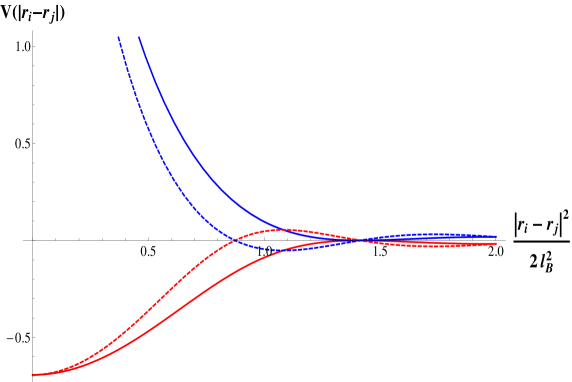
Figure 1: Statistical attraction potential (red line for symmetric states in the coordinates) and statistical repulsion potential (blue line for antisymmetric states in the coordinates) for electrons in graphene. $n_{i}=1$ and $n_{j}=1$ for continuous line and $n_{i}=2$ and $n_{j}=1$ for dashed line.

In the case of weak magnetic fields, the cutoff tends to $n_{\Delta}\rightarrow\infty$, then we can take the limit of large quantum numbers of the statistical potential (see [20], page 1003)

$$\underset{n_{i},n_{j}\rightarrow\infty}{\lim}V_{n_{i},n_{j}}(r_{i,}r_{j})\sim-\frac{1}{\beta}\ln(1\pm 4e^{-\frac{1}{2l_{B}^{2}}\left|r_{i}-r_{j}\right|^{2}}\frac{\sqrt{2}l_{B}}{\left|r_{i}-r_{j}\right|})$$ (20)

which differs from the interparticle statistical potential of eq.(9.57) of [16] for the Coulomb factor. An interesting result is that for antisymmetric states in the coordinates, the logarithm function diverges when the argument is zero, which gives the following equation for the minimum distance for the repulsive potential between electrons in the limit of weak magnetic fields and large quantum numbers

$$\ln\frac{x}{4}=-x^{2}$$ (21)

where $x=\frac{\left|r_{i}-r_{j}\right|}{2l_{B}}$. The solution of last equation is $x=\sqrt{W(2)/2}\sim 0.652$ where $W(x)$ is the Lambert $W$-function (see [21]), then $\left|r_{i}-r_{j}\right|>1.304l_{B}$.

As a final consideration for this section, we can introduce eq.(14) in eq.(6) and because the argument inside the integral do not depends on $s_{j}$, then the summation on this label can be done and the result reads

$$Z_{N}(\beta)=\sum\limits_{n_{1}=0}^{+n_{\Delta}}...\sum\limits_{n_{N}=0}^{+n_{\Delta}}\eta_{N}A_{n_{1},...,n_{N}}(N,\beta,\Omega)B_{n_{1},...,n_{N}}(N)$$ (22)

where

$$A_{n_{1},...,n_{N}}(N,\beta,\Omega)=2^{N}\overset{N}{\underset{j=1}{\prod}}\mu_{n}\cosh(\beta\Omega\sqrt{n_{j}})$$ (23)

where

$$\mu_{n}=(2-\delta_{n,0})^{-1}$$ (24)

and

$$B_{n_{1},...,n_{N}}(N)=\sum\limits_{p=0}^{N-1}\int(-1)^{p}\gamma_{n_{1},...,n_{N}}^{(p)}(r_{1},...,r_{N})d^{2}r_{1}...d^{2}r_{N}$$ (25)

In next sections, the first three terms of last equation will be obtained and general considerations will be done for the remaining terms.

2.1 $p=0$ permutation

If we consider no permutation in the coordinates, then the partition function reads

$$Z_{N}^{(0)}(\beta)=\sum\limits_{n_{1}=0}^{+n_{\Delta}}...\sum\limits_{n_{N}=0}^{+n_{\Delta}}2^{N}\overset{N}{\underset{j=1}{\prod}}\mu_{n}\cosh(\beta\Omega\sqrt{n_{j}})\eta_{N}L^{2N}2^{N}$$ (26)

where we have integrated in $d^{2}r_{j}$ and $L^{2}$ is the area of the graphene sheet. In this case, the function $\gamma_{n_{1},...,n_{N}}^{(0)}(r_{1},...,r_{N})$ reads

$$\gamma_{n_{1},...,n_{N}}^{(0)}(r_{1},...,r_{N})=L^{2N}2^{N}$$ (27)

We can separate each sum in $n_{j}$ and because they are equal we obtain

$$Z_{N}^{(0)}(\beta)=\eta_{N}2^{2N}L^{2N}\left(\sum\limits_{n=0}^{+n_{\Delta}}\mu_{n}\cosh\left(\beta\Omega\sqrt{n}\right)\right)^{N}$$ (28)

which is quite similar to the partition function of a magnetic system. From this partition function we can compute the entropy, the internal energy, the heat capacity and magnetization by using the Helmholtz free energy $F=-kT\ln Z_{N}$ by the following equations

$$S = -\frac{\partial F}{\partial T}\text{\ \ \ \ \ \ \ \ \ }M=-\frac{\partial F}{\partial B}$$ (29)

$$U = F+TS\text{ \ \ \ \ \ \ }C=\frac{\partial U}{\partial T}$$

In turn, using the Helmholtz free energy we can obtain the pressure of the thermodynamic system by the following equation $P=-\frac{\partial F}{\partial A}$, where $A=L^{2}$. Using the partition function obtained in eq.(28), the pressure for a gas of Bloch electrons in the classical limit of the partition function reads

$$PA=\frac{N}{2}kT$$ (30)

which is almost identical to state equation for and ideal gas in two dimension.

2.2 One permutation $p=1$

For one permutation, we have to take into account the function $\gamma_{n_{1},...,n_{N}}^{(1)}(r_{1},...,r_{N})$ which can be integrated in the coordinates

$$\int\gamma_{n_{1},...,n_{N}}^{(1)}(r_{1},...,r_{N})d^{2}r_{1}...d^{2}r_{N}=L^{2(N-2)}2^{N-2}\sum\limits_{i=1}^{N}\sum\limits_{j=i+1}^{N}Q_{n_{i},n_{j}}$$ (31)

where

$$Q_{n_{i},n_{j}}=\int g_{n_{i}}(\left|r_{j}-r_{i}\right|^{2})g_{n_{j}}(\left|r_{i}-r_{j}\right|^{2})d^{2}r_{i}d^{2}r_{j}$$ (32)

The factor $L^{2(N-2)}2^{N-2}$ appears due to the integration of the non-permutted coordinates. The function $Q_{n_{i},n_{j}}$ of similar to eq.(8) of [22], which is used as an interaction potential for electrons within a single Landau level. This potential is determined by the relative strength of the Coulomb interaction within the $n$-Landau level and it is used to study the charge excitacions of quantum ferromagnetic states (see [23] and [24]). In fact, the integral of eq.(13) is the exact interaction potential between $N$ electrons at different Landau levels.Using the result of eq.(13) we can write $Q_{n_{i},n_{j}}$ as

$$Q_{n_{i},n_{j}}=\sum\limits_{l=0}^{1}\sum\limits_{k=0}^{1}W_{n_{i}-l,n_{j}-k}(1-\delta_{n_{i},0})^{l}(1-\delta_{n_{j},0})^{k}$$ (33)

where $W_{a,b}$ reads

$$W_{a,b}=\int e^{-\frac{1}{2l_{B}^{2}}\left|r_{i}-r_{j}\right|^{2}}L_{a}(\frac{1}{2l_{B}^{2}}\left|r_{i}-r_{j}\right|^{2})L_{b}(\frac{1}{2l_{B}^{2}}\left|r_{i}-r_{j}\right|^{2})d^{2}r_{i}d^{2}r_{j}$$ (34)

writing $\left|r_{i}-r_{j}\right|^{2}=(x_{i}-x_{j})^{2}+(y_{i}-y_{j})^{2}$ and making the following center of mass coordinate transformation

$$x_{i}-x_{j} = x_{ij}\text{ \ \ \ \ \ \ \ \ \ }X_{ij}=\frac{1}{2}(x_{i}+x_{j})$$ (35)

$$y_{i}-y_{j} = y_{ij}\text{ \ \ \ \ \ \ \ \ \ }Y_{ij}=\frac{1}{2}(y_{i}+y_{j})$$

then

$$W_{a,b}=L^{2}\int e^{-\frac{1}{2l_{B}^{2}}(x_{ij}^{2}+y_{ij}^{2})}L_{a}(\frac{1}{2l_{B}^{2}}(x_{ij}^{2}+y_{ij}^{2}))L_{b}(\frac{1}{2l_{B}^{2}}(x_{ij}^{2}+y_{ij}^{2}))dx_{ij}dy_{ij}$$ (36)

where the area $L^{2}$ appears due to the $dX_{ij}$ and $dY_{ij}$ integration. Finally, using polar coordinates $x_{ij}=r_{ij}\cos\theta_{ij}$ and $y_{ij}=r_{ij}\sin\theta_{ij}$, and performing the $\theta_{ij}$ integration we obtain

$$W_{a,b}=2\pi L^{2}\int e^{-\frac{r_{ij}^{2}}{2l_{B}^{2}}}L_{a}(\frac{r_{ij}^{2}}{2l_{B}^{2}})L_{b}(\frac{r_{ij}^{2}}{2l_{B}^{2}})r_{ij}dr_{ij}$$ (37)

finally, making the coordinate transformation $s=r_{ij}^{2}/2l_{B}^{2}$ the function $W_{a,b}$ reads

$$W_{a,b}=2\pi(Ll_{B})^{2}\int e^{-s}L_{a}(s)L_{b}(s)ds$$ (38)

using the orthogonality of the Laguerre polynomials we obtain

$$W_{a,b}=2\pi(Ll_{B})^{2}\int e^{-s}L_{a}(s)L_{b}(s)ds=2\pi(Ll_{B})^{2}\delta_{ab}$$ (39)

Replacing this last result in eq.(32) we obtain

$$Q_{n_{i},n_{j}}=\sum\limits_{l=0}^{1}\sum\limits_{k=0}^{1}W_{n_{i}-l,n_{j}-k}(1-\delta_{n_{i},0})^{l}(1-\delta_{n_{j},0})^{k}=2\pi(Ll_{B})^{2}\sum\limits_{l=0}^{1}\sum\limits_{k=0}^{1}\delta_{n_{i}-l,n_{j}-k}(1-\delta_{n_{i},0})^{l}(1-\delta_{n_{j},0})^{k}$$ (40)

Then the partition function with the correction given by one permutation reads

$$Z_{N}^{(1)}(\beta)=\sum\limits_{n_{1}=0}^{+n_{\Delta}}...\sum\limits_{n_{N}=0}^{+n_{\Delta}}2^{N}\overset{N}{\underset{j=1}{\prod}}\mu_{n}\cosh(\beta\Omega\sqrt{n_{j}})\eta_{N}\times$$ (41)

$$\left(L^{2N}2^{N}+\frac{\pi}{2}L^{2(N-1)}2^{N-2}l_{B}^{2}\sum\limits_{i=1}^{N}\sum\limits_{j=i+1}^{N}\sum\limits_{l=0}^{1}\sum\limits_{k=0}^{1}\delta_{n_{i}-l,n_{j}-k}(1-\delta_{n_{i},0})^{l}(1-\delta_{n_{j},0})^{k}\right)$$

By doing some complex algebraic manipulations is possible to obtain a exact description of the contribution of one permutation to the partition function, which reads

$$Z_{N}^{(1)}(\beta)=Z_{N}^{(0)}(\beta)\left(1+\frac{\pi}{8}\frac{l_{B}^{2}}{L^{2}}F_{1}(\beta,\Omega,N)\right)$$ (42)

where

$$F_{1}(\beta,\Omega,N)=N(N-1)\frac{\sum\limits_{n=0}^{+n_{\Delta}}\mu_{n}\cosh^{2}(\beta\Omega\sqrt{n})+\sum\limits_{n=1}^{+n_{\Delta}}\mu_{n}\mu_{n-1}\cosh(\beta\Omega\sqrt{n})\cosh(\beta\Omega\sqrt{n-1})-1/2}{\left(\sum\limits_{n=0}^{+n_{\Delta}}\mu_{n}\cosh(\beta\Omega\sqrt{n})\right)^{2}}$$ (43)

The correction introduced by eq.(43) can be used to obtain the thermodynamic functions and to compare it with the results obtained in last subsection.

2.3 Two permutation $p=2$

The contribution to the partition function of two permutations is computed. In this case, an interesting effect appears due to the gauge dependent term $\sigma$ when we take into account two permutations

$$\int\gamma_{n_{1},...,n_{N}}^{(2)}(r_{1},...,r_{N})d^{2}r_{1}...d^{2}r_{N}=L^{2(N-3)}2^{N-3}\times$$ (44)

$$\sum\limits_{i=1}^{N}\sum\limits_{j=i+1}^{N}\sum\limits_{k=j+1}^{N}U_{n_{i},n_{j},n_{k}}$$

where

$$U_{n_{i},n_{j},n_{k}}=\int g_{n_{i}}(\left|r_{j}-r_{i}\right|^{2})g_{n_{j}}(\left|r_{k}-r_{j}\right|^{2})g_{n_{k}}(\left|r_{i}-r_{k}\right|^{2})\cos(\sigma(r_{j},r_{i})+\sigma(r_{k},r_{j})+\sigma(r_{i},r_{k})))d^{2}r_{i}d^{2}r_{j}d^{2}r_{k}$$ (45)

Last equation prevents to consider the statistical potential of eq.(19) beyond the first order in the perturbation expansion due to the gauge dependent term $\sigma$ that appears when we consider at least three particles. Using eq.(9), the argument of the cosine function reads

$$\sigma(r_{j},r_{i})+\sigma(r_{k},r_{j})+\sigma(r_{i},r_{k})=\frac{1}{2l_{B}^{2}}\left(y_{j}x_{i}-y_{i}x_{j}+y_{k}x_{j}-y_{j}x_{k}+y_{i}x_{k}-y_{k}x_{i}\right)$$ (46)

which can be rewritten in terms of skew products between position vectors

$$\sigma(r_{j},r_{i})+\sigma(r_{k},r_{j})+\sigma(r_{i},r_{k})=\frac{1}{2l_{B}^{2}}\left(\overrightarrow{r}_{j}\times\overrightarrow{r}_{i}+\overrightarrow{r}_{k}\times\overrightarrow{r}_{j}+\overrightarrow{r}_{i}\times\overrightarrow{r}_{k}\right)\widehat{e}_{z}$$ (47)

Introducing the following coordinate transformation

$$\overrightarrow{r}_{ji}=\overrightarrow{r}_{j}-\overrightarrow{r}_{i}$$ (48)

$$\overrightarrow{r}_{kj}=\overrightarrow{r}_{k}-\overrightarrow{r}_{j}$$

$$\overrightarrow{R}=\overrightarrow{r}_{i}+\overrightarrow{r}_{j}+\overrightarrow{r}_{k}$$

eq.(44) reads

$$U_{n_{i},n_{j},n_{k}}=\frac{1}{3}\int g_{n_{i}}(\left|\overrightarrow{r}_{ji}\right|^{2})g_{n_{j}}(\left|\overrightarrow{r}_{kj}\right|^{2})g_{n_{k}}(\left|\overrightarrow{r}_{ji}+\overrightarrow{r}_{kj}\right|^{2})\cos(\frac{1}{6l_{B}^{2}}\left(\overrightarrow{r}_{kj}\times\overrightarrow{r}_{ji}\right)\widehat{e}_{z})d^{2}r_{ji}d^{2}r_{kj}d^{2}R$$ (49)

finally we can introduce polar coordinates

$$x_{ji} = r_{ji}\cos\theta_{ji}\text{ \ \ \ \ \ \ \ \ \ }y_{ji}=r_{ji}\sin\theta_{ji}$$ (50)

$$\text{\ }x_{kj} = r_{kj}\cos\theta_{kj}\text{ \ \ \ \ \ \ \ \ }y_{kj}=r_{kj}\sin\theta_{kj}$$

then, eq.(49) reads

$$U_{n_{i},n_{j},n_{k}}=\sum\limits_{r=0}^{1}\sum\limits_{s=0}^{1}\sum\limits_{t=0}^{1}u_{n_{i}-r,n_{j}-s,n_{k}-t}(1-\delta_{n_{i},0})^{r}(1-\delta_{n_{j},0})^{s}(1-\delta_{n_{k},0})^{t}$$ (51)

where

$$u_{a,b,c}=\frac{L^{2}}{3}\int L_{a}(r_{ji}^{2})L_{b}(r_{kj}^{2})L_{c}((r_{ji}+r_{kj})^{2})\cos(\frac{1}{6l_{B}^{2}}r_{kj}r_{ji}\sin(\theta_{ji}-\theta_{kj}))r_{ji}dr_{ji}d\theta_{ji}r_{kj}dr_{kj}d\theta_{kj}$$ (52)

introducing the coordinates $s_{ji}=r_{ji}^{2}/2l_{B}^{2}$, $s_{kj}=r_{kj}^{2}/2l_{B}^{2}$, $\gamma=\theta_{ji}-\theta_{kj}$ and $\nu=\theta_{ji}+\theta_{kj}$ and integrating over this last variable we obtain

$$u_{a,b,c}=\frac{\pi L^{2}l_{B}^{4}}{3}T_{a,b,c}$$ (53)

where

$$T_{a,b,c}=\int e^{-(\sqrt{s_{ji}}+\sqrt{s_{kj}})^{2}}L_{a}(s_{ji})L_{b}(s_{kj})L_{c}((\sqrt{s_{ji}}+\sqrt{s_{kj}})^{2})\cos(\frac{\sqrt{s_{ji}s_{kj}}}{3}\sin(\gamma))ds_{ij}ds_{kj}d\gamma$$ (54)

We can perform the $\gamma$ integration

$$\int_{0}^{2\pi}\cos(\frac{\sqrt{s_{ji}s_{kj}}}{3}\sin(\gamma))d\gamma=2\pi J_{0}(\frac{\sqrt{s_{ji}s_{kj}}}{3})$$ (55)

then

$$T_{a,b,c}=2\pi\int e^{-(\sqrt{s_{ji}}+\sqrt{s_{kj}})^{2}}L_{a}(s_{ji})L_{b}(s_{kj})L_{c}((\sqrt{s_{ji}}+\sqrt{s_{kj}})^{2})J_{0}(\frac{\sqrt{s_{ji}s_{kj}}}{3})ds_{ij}ds_{kj}$$ (56)

This last integral is not computed in the work because of their complexity. Taking into account all the terms of the sum in eq.(44), the two permutation contribution to the partition function reads

$$\int\gamma_{n_{1},...,n_{N}}^{(2)}(r_{1},...,r_{N})d^{2}r_{1}...d^{2}r_{N}=L^{2(N-3)}2^{N-3}\frac{\pi L^{2}l_{B}^{4}}{3}\times$$ (57)

$$\sum\limits_{i=1}^{N}\sum\limits_{j=1+1}^{N}\sum\limits_{k=j+1}^{N}\sum\limits_{r=0}^{1}\sum\limits_{s=0}^{1}\sum\limits_{t=0}^{1}T_{n_{i}-r,n_{j}-s,n_{k}-t}(1-\delta_{n_{i},0})^{r}(1-\delta_{n_{j},0})^{s}(1-\delta_{n_{k},0})^{t}$$

and the partition function with the two permutation contribution reads

$$Z_{N}(\beta)=\left(\sum\limits_{n=0}^{+n_{\Delta}}\cosh(\beta\Omega\sqrt{n})\right)^{N}\eta_{N}L^{2N}\left(1+\frac{\pi}{2L^{2}}2^{N-2}l_{B}^{2}F_{1}(\beta,\Omega,N)+\frac{\pi 2^{N-3}l_{B}^{4}}{3L^{4}}F_{2}(\beta,\Omega,N)\right)$$ (58)

where

$$F_{2}(\beta,\Omega,N)=\frac{\sum\limits_{n_{1}=0}^{+n_{\Delta}}...\sum\limits_{n_{N}=0}^{+n_{\Delta}}\overset{N}{\underset{j=1}{\prod}}\cosh(\beta\Omega\sqrt{n_{j}})\sum\limits_{i=1}^{N}\sum\limits_{j=1+1}^{N}\sum\limits_{k=j+1}^{N}\sum\limits_{r=0}^{1}\sum\limits_{s=0}^{1}\sum\limits_{t=0}^{1}T_{n_{i}-r,n_{j}-s,n_{k}-t}}{\left(\sum\limits_{n=0}^{+n_{\Delta}}\cosh(\beta\Omega\sqrt{n})\right)^{N}}$$ (59)

In this case, the sum has not been performed because we cannot solve eq.(56). The gauge dependent term $\sigma$ inhibit to consider the statistical potential beyond one permutation and then has to be considered an approximation, not only by the condition $\left|r_{i}-r_{j}\right|>l_{B}$, but also for the correlation between three or more electrons considered at once.

3 Results and discussion

We can use eq.(42) to compute thermodynamic functions. The effective long wavelength approximation of the electron dynamics in graphene in a uniform magnetic field is valid only at low energies, i.e. for low-lying Landau levels as it was shown in the introduction. The properties of higher Landau levels can be described within the tight-binding model by introducing the Peierls substitution (see [25] and [26]). In particular, we can consider an intense magnetic field in such a way that the cutoff $n_{\Delta}$ is $n_{\Delta}\sim 1000$. This implies that $B\sim\frac{4\pi\hbar}{10^{3}3\sqrt{3}a^{2}e}\sim 100T$ which are magnetic fields that can be obtained in laboratory. In particular, we will consider only two particles, $N=2$, in this way, the correction to the partition function of eq.(42) gives the total partition function of the system.

Using the definition of the thermodynamic functions of eq.(29) we can obtain the entropy, the internal energy, the specific heat and magnetization for a quantum system composed of two Bloch electrons in a high magnetic field for symmetric and antisymmetric states in the coordinates. In figure 2, 3, 4 and 5 it is shown the results obtained with the partition function $Z_{2}^{(0)}(\beta)$ (black line in figures) and the partition function $Z_{2}^{(1)}(\beta)$ with the one permutation correction (red dashed line for antisymmetric states and blue dashed line for symmetric states in figures). In all the cases, the thermodynamic functions are plotted against temperature in the range from $0$ to $1000$ K.

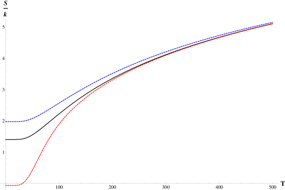
Figure 2: Entropy as a function of the temperature. Without exchange correlation (red line) and with exchange correlation (blue line). The black line shows entropy without permutation correction.

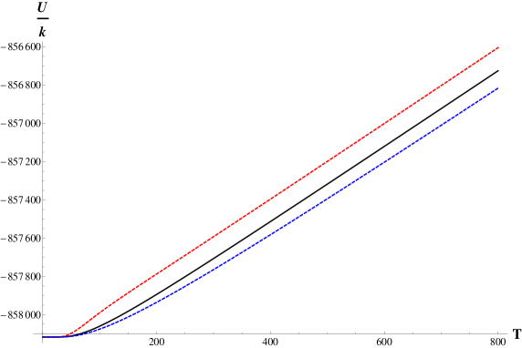
Figure 3: Internal energy as a function of the temperature. Without exchange correlation (red line) and with exchange correlation (blue line). The black line shows entropy without permutation correction.

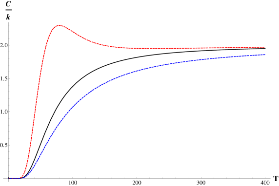
Figure 4: Capacity heat as a function of the temperature. Without exchange correlation (red line) and with exchange correlation (blue line). The black line shows entropy without permutation correction.

As it can be seen in figure 2, the entropy of the quantum system without interaction between Bloch electrons is larger than the entropy of the same system in an anstisymmetric state and lower than the entropy of the same system in a symmetric state in the coordinates. At higher temperatures, both entropies match, which implies that disorder erase the exchange correlation between electrons. At low temperatures, the difference between entropies between antisymmetric states and symmetric states can be understood due to the simple fact that there are more symmetric available states than antisymmetric. The lowest energy value is $-2\Omega\sqrt{n_{\Delta}}$, which cannot support an antisymmetric state because it is zero but it does support a symmetric state. As we move through the possible energy levels of the composite system, more symmetric than antisymmetric states are available. In fact, there are $(2n_{\Delta}+1)(2n_{\Delta}+2)/2$ symmetric states and $(2n_{\Delta}+1)n_{\Delta}$ antisymmetric states available in the spectrum. In turn, the internal energy (see figure 3) for antisymmetric states is larger than the internal energy of the same system in a symmetric state. This is related to energy of the lowest antisymmetric state available which is $E=-\Omega(\sqrt{n_{\Delta}}+\sqrt{n_{\Delta}+1})$. The specific heat (see figure 4) of both statististics has a limit behavior as $T\rightarrow\infty$, which correspond to entropy saturation due to the upper bound in the energy levels. But the specific heat of antisymmetric states has a peak, the Schottky anomaly, which is related to the larger separation between consecutive energy values available (see [27]). In [15], the specific heat is computed with doped graphene in a magnetic field. In this case, the specific heat shows a Schottky anomaly, but this is related to the band gap between conduction and valence band introduced by the impurities (see [28]).

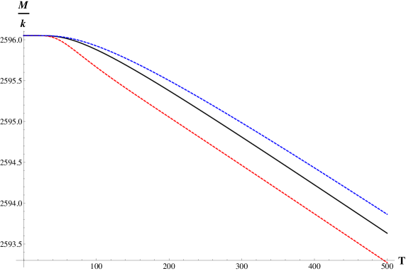
Figure 5: Magnetic susceptibility as a function of temperature.Without exchange correlation (red line) and with exchange correlation (blue line). The black line shows entropy without permutation correction.

The magnetization (see Figure 5) shows a typical behavior of a magnetic system, but in this case, the degrees of freedom that make the role of spins are the conduction and valence bands. From the figure, the magnetic susceptibility is negative and correspond to the ferromagnetic phase of graphene in a magnetic field.

Finally, using the Helmholtz free energy, we can obtain the pressure of the thermodynamic system by the following equation $P=-\frac{\partial F}{\partial A}$, where $A=L^{2}$. The general result reads

$$P=kT\left[\frac{N}{2A}-\frac{\frac{\pi}{8}l_{B}^{2}F_{1}(\frac{1}{kT},\Omega,N)}{A^{2}+\frac{\pi}{8}Al_{B}^{2}F_{1}(\frac{1}{kT},\Omega,N)}\right]$$ (60)

Using this last result for $N=3$,  since with two particles, the correction do not depend on $L^{2}$, the quantum pressure can be plotted against temperature as it is shown in figure 6.

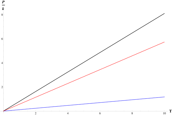
Figure 6: Pressure as a function of temperature. The black line shows entropy without permutation correction.

As we can see in figure 6, the pressure tends to zero as $T\rightarrow 0$. A quantum degeneracy pressure would be expected, but the degeneracy of fermions in graphene in a constant magnetic field introduce an statistical potential that allows fermions to behave as attractive particles at low temperature.

Due to the unusual thermal properties of electrons in graphene found in last section when the exchange correlation term is considered in the partition function, where an attractive statistical potential can be obtained, it would be interesting to study the interaction between graphene-semiconductor junction in the depletion region to see if there is any particular behavior of the Schottky barrier. Theoretical and experimental works has been done in this line of work (see [29], [30], [31] and [32]).

4 General considerations

We can infer a general result for the succesive terms of the perturbation expansion of the partition function that depends on the factor $\lambda=\frac{l_{B}}{L}\,$. The partition function can be written in a general form as

$$Z_{N}(\beta)=\sum\limits_{n_{1}=0}^{+n_{\Delta}}...\sum\limits_{n_{N}=0}^{+n_{\Delta}}A_{n_{1},...,n_{N}}(N,\beta,\Omega)\eta_{N}L^{2N}2^{N}\sum\limits_{p=0}^{N-1}2^{-p}\lambda^{p}C_{p}(N)$$ (61)

A factor $L^{2(N-p)}2^{N-p}$ comes from the $g_{n}$ function integration that contains no permutation in its arguments. A $L^{2}l_{B}^{2p}$ factor comes from the change of variable $s=r^{2}/2l_{B}^{2}$, where $L^{2}$ is due to the center of mass variable integration. The coefficients $C_{p}(N)$ contains the results given by the integral of the $g_{n}$ functions with the permuted arguments and for the first three coefficients we have obtained

$$C_{0}(N)=1\text{, \ \ \ \ }C_{1}(N)=2\pi\sum\limits_{i=1}^{N}\sum\limits_{j=i+1}^{N}\sum\limits_{l=0}^{1}\sum\limits_{k=0}^{1}\delta_{n_{i}-l,n_{j}-k}\text{\ }(1-\delta_{n_{i},0})^{l}(1-\delta_{n_{j},0})^{k}$$ (62)

$$C_{2}(N)=2\pi\sum\limits_{i=1}^{N}\sum\limits_{j=1+1}^{N}\sum\limits_{k=j+1}^{N}\sum\limits_{r=0}^{1}\sum\limits_{s=0}^{1}\sum\limits_{t=0}^{1}T_{n_{i}-r,n_{j}-s,n_{k}-t}(1-\delta_{n_{i},0})^{r}(1-\delta_{n_{j},0})^{s}(1-\delta_{n_{k},0})^{t}$$

where $T_{n_{i}-r,n_{j}-s,n_{k}-t}$ is defined in eq.(56). The factor $\eta_{N}L^{2N}$ in eq.(61) contains the constant $\lambda^{-N}$ which is common for all the terms.

The gauge dependent term $\sigma$ prevent us to understand the statistical potential beyond one permutation. In turn, we cannot apply a cluster expansion, where we separate particles that are close together from another cluster because the cosine function in eq.(13) contains the skew product between position vectors. The unique possible way in which the argument of the cosine function is zero is only when the particles are aligned, but this is a very specific configuration of particles in graphene sheet. In the case of two permutations, the vanishing of the cosine function is translated to the vanishing of the Bessel function $J_{0}$, where the argument is $r_{ji}r_{kj}/6l_{B}^{2}$.

5 Conclusion

In this paper we have studied the thermodynamics properties of non-interacting Bloch electrons in graphene in a constant magnetic field computing the internal energy, specific heat, entropy and magnetic susceptibility at zero and one order of the constant $l_{B}/L$ in the perturbation expansion of the partition function and we have sketch the term that contributes to second order. We have shown that at first order, the partition function can be written as a system of $N$ Bloch electrons with a attractive statistical potential for certain values of the interparticle distance. Thermodynamic functions has been computed and compared between no permutation and one permutation contribution for antisymmetric and symmetric states. Due to the larger microstates available for symmetric states, entropy increase its value with respect to same quantum system without one permutation correction. Internal energy is lower for antisymmetric states showing the effect of exchange correlation and the specific heat present a Schottky anomaly due to the large gaps between energy levels available for antisymmetric states. Graphene in a magnetic field present a magnetic behavior, although no spin-orbit interaction has been taken into account. The conducion and valence band acts as spin in graphene and couples to the magnetic field with $\sqrt{B}$ dependence.

6 Acknowledgment

This paper was partially supported by grants of CONICET (Argentina National Research Council) and Universidad Nacional del Sur (UNS) and by ANPCyT through PICT 1770, and PIP-CONICET Nos. 114-200901-00272 and 114-200901-00068 research grants, as well as by SGCyT-UNS., E.A.G. and P.V.J. are members of CONICET. P.B. and J. S.A. are fellow researchers at this institution.

7 Appendix

Suppose that our system consist of $N$ non-interacting Bloch electrons in graphene in the long wavelength approximation, placed in a constant magnetic field perpendicular to the graphene sheet. The eigenfunctions of the Hamiltonian are those of eq.(2) where the energies are those of eq.(5).

The partition function of the system reads

$$Z_{N}(\beta)=Tr(e^{-\beta H})=\int\left\langle r_{1},..,r_{N}\left|e^{-\beta H}\right|r_{1},..,r_{N}\right\rangle d^{2}r_{1}...d^{2}r_{N}$$ (63)

The eigenfunctions contain three indices, the quantum harmonic oscillator index $n=0,1,2,...,n_{\Delta}$, the conduction and valence band $s=\pm 1$ and the wave vector $k$ in the $x$ direction. With these eigenfunctions we can define an identity operator for a quantum system

$$I=\sum\limits_{s=-1}^{+1}\sum\limits_{n=0}^{+n_{\Delta}}\int dk\left|n,s,k\right\rangle\left\langle n,s,k\right|$$ (64)

We can introduce the identity for each quantum system in the partition function, then

$$Z_{N}(\beta)=\sum\limits_{s_{1}=-1}^{+1}...\sum\limits_{s_{N}=-1}^{+1}\sum\limits_{n_{1}=0}^{+n_{\Delta}}...\sum\limits_{n_{N}=0}^{+n_{\Delta}}\exp(-\beta\sum\limits_{j=1}^{N}E_{n_{j},s_{j}})\times$$ (65)

$$\int dk_{1}...dk_{N}\Phi_{\alpha_{1},...,\alpha_{N}}^{\ast}(r_{1},...,r_{N})\Phi_{\alpha_{1},...,\alpha_{N}}(r_{1},...,r_{N})d^{2}r_{1}...d^{2}r_{N}$$

where $\alpha_{j}=\{n_{j},s_{j},k_{j}\}$ are the index collection for the Bloch electrons in graphene and

$$\Phi_{\alpha_{1},...,\alpha_{N}}(r_{1},...,r_{N})=\frac{1}{\sqrt{N!}}\sum\limits_{P}\delta_{P}P\{\psi_{\alpha_{1}}(r_{1})...\psi_{\alpha_{N}}(r_{N})\}$$ (66)

where $\delta_{P}$ is $+1$ or $-1$ according as the permutation $P$ of the single-particle wave functions $\psi_{\alpha_{j}}(r_{j})$ defined on eq.(2) is even or odd, that is $\delta_{P}=(-1)^{[P]}$, where $[P]$ denotes the order of the permutation. The factor $(N!)^{-1/2}$ is introduced to secure the normalization of the total wave function. Introducing eq.(66) in eq.(65) we have

$$Z_{N}(\beta)=\sum\limits_{s_{1}=-1}^{+1}...\sum\limits_{s_{N}=-1}^{+1}\sum\limits_{n_{1}=0}^{+n_{\Delta}}...\sum\limits_{n_{N}=0}^{+n_{\Delta}}\exp(-\beta\sum\limits_{j=1}^{N}E_{n_{j},s_{j}})\times\int\chi_{\alpha_{1},...,\alpha_{N}}(r_{1},...,r_{N})d^{2}r_{1}...d^{2}r_{N}$$ (67)

where

$$\chi_{\alpha_{1},...,\alpha_{N}}(r_{1},...,r_{N})=\frac{1}{N!}\int dk_{1}...dk_{N}\sum\limits_{P}\sum\limits_{P^{\prime}}\delta_{P}\delta_{P^{\prime}}[\psi_{\alpha_{1}}^{\ast}(Pr_{1})\psi_{\alpha_{1}}(P^{\prime}r_{1})...\psi_{\alpha_{N}}^{\ast}(Pr_{N})\psi_{\alpha_{N}}(P^{\prime}r_{N})]$$ (68)

Taking outside the sum in $P$ and $P^{\prime}$ in last equation

$$\chi_{\alpha_{1},...,\alpha_{N}}(r_{1},...,r_{N})=\frac{1}{N!}\sum\limits_{P}\sum\limits_{P^{\prime}}\delta_{P}\delta_{P^{\prime}}\overset{N}{\underset{j=1}{\prod}}f_{\alpha_{j}}(Pr_{j},P^{\prime}r_{j})$$ (69)

where

$$f_{\alpha_{j}}(Pr_{j},P^{\prime}r_{j})=\int dk_{j}\psi_{\alpha_{j}}^{\ast}(Pr_{j})\psi_{\alpha_{j}}(P^{\prime}r_{j})$$ (70)

is a function of the coordinates and can be evaluated by replacing eq.(2) into last equation

$$f_{\alpha_{j}}(Pr_{j},P^{\prime}r_{j})=\frac{\left|C_{n_{j}}\right|^{2}}{2L}\int dk_{j}e^{ik_{j}(P^{\prime}x_{j}-Px_{j})}\varphi_{(n_{j},s_{j},k_{j})}^{T}(P\xi_{j})\varphi_{(n_{j},s_{j},k_{j})}(P^{\prime}\xi_{j})$$ (71)

where $\varphi_{(n_{j},s_{j},k_{j})}(\xi_{j})$ is defined on eq.(3). Introducing eq.(3) on eq.(71) we obtain

$$f_{\alpha_{j}}(Pr_{j},P^{\prime}r_{j})=\frac{1}{2(2-\delta_{n_{j},0})L}\times$$ (72)

$$\int dk_{j}e^{ik_{j}(P^{\prime}x_{j}-Px_{j})}(2s_{j}^{2}\phi_{n_{j}-1,k_{j}}^{\ast}(P\xi_{j})\phi_{n_{j}-1,k_{j}}(P^{\prime}\xi_{j})(1-\delta_{n_{j},0})+2\phi_{n_{j},k_{j}}^{\ast}(P\xi_{j})\phi_{n_{j},k_{j}}(P^{\prime}\xi_{j}))$$

and using eq.(4)

$$f_{\alpha_{j}}(Pr_{j},P^{\prime}r_{j})=\frac{\pi^{-1/2}}{(2-\delta_{n_{j},0})L}\int dk_{j}e^{ik_{j}(P^{\prime}x_{j}-Px_{j})}\times$$ (73)

$$(\frac{s_{j}^{2}}{2^{n_{j}-1}(n_{j}-1)!}e^{-\frac{1}{2}((P\xi_{j})^{2}+(P^{\prime}\xi_{j})^{2})}H_{n_{j-1,k_{j}}}(P\xi_{j})H_{n_{j-1,k_{j}}}(P^{\prime}\xi_{j})(1-\delta_{n_{j},0})+$$

$$\frac{1}{2^{n_{j}}n_{j}!}e^{-\frac{1}{2}((P\xi_{j})^{2}+(P^{\prime}\xi_{j})^{2})}H_{n_{j,k_{j}}}(P\xi_{j})H_{n_{j,k_{j}}}(P^{\prime}\xi_{j}))$$

Completing squares in the exponentials we obtain for the first integral in last equation

$$f_{\alpha_{j}}^{(1)}(Pr_{j},P^{\prime}r_{j})=\frac{s_{j}^{2}\pi^{-1/2}e^{b}}{(2-\delta_{n_{j},0})L2^{n_{j}-1}(n_{j}-1)!}\times$$ (74)

$$\int dk_{j}e^{-(l_{B}k_{j}-l_{B}a)^{2}}H_{n_{j-1,k_{j}}}(\frac{Py_{j}}{l_{B}}-l_{B}k_{j})H_{n_{j-1,k_{j}}}(\frac{y_{j}}{l_{B}}-l_{B}k_{j})$$

where the supperscript in $f_{\alpha_{j}}^{(1)}(Pr_{j},P^{\prime}r_{j})$ indicate the first integral of eq.(73) and

$$b(Px_{j},P^{\prime}x_{j},Py_{j},P^{\prime}y_{j})=\frac{(Py_{j}+P^{\prime}y_{j}+i(P^{\prime}x_{j}-Px_{j}))^{2}}{4l_{B}^{2}}-\frac{1}{2l_{B}^{2}}((Py_{j})^{2}+(P^{\prime}y_{j})^{2})$$ (75)

and

$$a(Px_{j},P^{\prime}x_{j},Py_{j},P^{\prime}y_{j})=\frac{(Py_{j}+P^{\prime}y_{j}+i(P^{\prime}x_{j}-Px_{j}))}{2l_{B}^{2}}$$ (76)

By introducing the following coordinate transformation

$$q_{j}=\frac{Py_{j}}{l_{B}}-l_{B}k_{j}$$ (77)

eq.(74) reads

$$f_{\alpha_{j}}^{(1)}(Pr_{j},P^{\prime}r_{j})=-\frac{s_{j}^{2}\pi^{-1/2}e^{b}}{(2-\delta_{n_{j},0})Ll_{B}2^{n_{j}-1}(n_{j}-1)!}\times$$ (78)

$$\int dq_{j}e^{-(\frac{Py_{j}}{l_{B}}-q_{j}-l_{B}a)^{2}}H_{n_{j-1,k_{j}}}(q_{j})H_{n_{j-1,k_{j}}}(\frac{P^{\prime}y_{j}}{l_{B}}+q_{j}-\frac{Py_{j}}{l_{B}})$$

A second coordinate transformation can be applied

$$-z_{j}=\frac{Py_{j}}{l_{B}}-q_{j}-l_{B}a$$ (79)

that change eq.(78) in

$$f_{\alpha_{j}}^{(1)}(Pr_{j},P^{\prime}r_{j})=-\frac{s_{j}^{2}\pi^{-1/2}e^{b}}{(2-\delta_{n_{j},0})Ll_{B}2^{n_{j}-1}(n_{j}-1)!}\times$$ (80)

$$\int dz_{j}e^{-z_{j}^{2}}H_{n_{j-1,k_{j}}}(\frac{Py_{j}}{l_{B}}-l_{B}a+z_{j})H_{n_{j-1,k_{j}}}(\frac{y_{j}}{l_{B}}+z_{j}-l_{B}a)$$

Using eq.(7.377⁸) of page 804 of [20]

$$\int e^{-x^{2}}H_{m}(x+y)H_{n}(x+z)dx=2^{n}\pi^{1/2}m!z^{n-m}L_{m}^{n-m}(-2yz)$$ (81)

where $m\leq n$ and $L_{m}^{n-m}(x)$ is the associated Laguerre polynomial, eq.(80) reads

$$f_{\alpha_{j}}^{(1)}(Pr_{j},P^{\prime}r_{j})=-\frac{s_{j}^{2}e^{b}}{(2-\delta_{n_{j},0})Ll_{B}}L_{n_{j}-1}(-2(\frac{Py_{j}}{l_{B}}-l_{B}a)(\frac{P^{\prime}y_{j}}{l_{B}}-l_{b}a))$$ (82)

Finally, taking into account that the same result is obtained in the second integral in eq.(73) with the $n_{j}-1\rightarrow n_{j}$ replacement, eq.(80) reads

$$f_{\alpha_{j}}(Pr_{j},P^{\prime}r_{j})=-\frac{e^{b}}{(2-\delta_{n_{j},0})Ll_{B}}\times$$ (83)

$$\left(L_{n_{j}-1}(-2(\frac{Py_{j}}{l_{B}}-l_{B}a)(\frac{P^{\prime}y_{j}}{l_{B}}-l_{b}a))(1-\delta_{n_{j},0})+L_{n_{j}}(-2(\frac{Py_{j}}{l_{B}}-l_{B}a)(\frac{P^{\prime}y_{j}}{l_{B}}-l_{b}a))\right)$$

by doins some algebraic manipulations we can rewrite the argument of the Laguerre polynomials as

$$-2(\frac{Py_{j}}{l_{B}}-l_{B}a)(\frac{P^{\prime}y_{j}}{l_{B}}-l_{B}a)=\frac{1}{2l_{B}^{2}}\left|P^{\prime}r_{j}-Pr_{j}\right|^{2}$$ (84)

where $Pr_{j}=(Px_{j},Py_{j})$. In turn, the $b$ function can be written as

$$b=-\frac{1}{4l_{B}^{2}}(\left|Pr_{j}-P^{\prime}r_{j}\right|^{2})+i\sigma$$ (85)

where $\sigma$ is the gauge-dependent term which reads

$$\sigma(Pr_{j},P^{\prime}r_{j})=\frac{1}{2l_{B}^{2}}((P^{\prime}y_{j}+Py_{j})(P^{\prime}x_{j}-Px_{j}))$$ (86)

Using these results, the function $f_{\alpha_{j}}(Pr_{j},P^{\prime}r_{j})$ finally reads

$$f_{\alpha_{j}}(Pr_{j},P^{\prime}r_{j})=-\frac{e^{-\frac{1}{4l_{B}^{2}}\left|Pr_{j}-P^{\prime}r_{j}\right|^{2}+i\sigma}}{(2-\delta_{n_{j},0})Ll_{B}}\times$$ (87)

$$\left[L_{n_{j}-1}(\frac{1}{2l_{B}^{2}}\left|Pr_{j}-P^{\prime}r_{j}\right|^{2})(1-\delta_{n_{j},0})+L_{n_{j}}(\frac{1}{2l_{B}^{2}}\left|Pr_{j}-P^{\prime}r_{j}\right|^{2})\right]$$

This result will be used in the main sections of this paper.

References

- [1] K. S. Novoselov, A. K. Geim, S. V. Morozov, D. Jiang, M. I. Katsnelson, I. V. Grigorieva, S. V. Dubonos and A. A. Firsov, Nature, 438, 197 (2005).
- [2] A.K. Geim and K. S. Novoselov, Nature Materials, 6, 183 (2007).
- [3] Y. B. Zhang, Y.W. Tan, H. L. Stormer and P. Kim, Nature, 438, 201 (2005).
- [4] A. H. Castro Neto, F. Guinea, N. M. R. Peres, K. S. Novoselov and A. K. Geim, Rev. Mod. Phys., 81, 109 (2009).
- [5] M. O. Goerbig, Rev. Mod. Phys., 83, 4, (2011).
- [6] J. McClure, Phys. Rev., 104, 666 (1956).
- [7] S. Kuru, J. Negro and L. M. Nieto, J. Phys.: Condens. Matter, 21, 455305 (2009).
- [8] Y. Zheng and T. Ando, Phys. Rev. B, 65, 245420 (2002).
- [9] A. Matulis and F. M. Peters, Phys. Rev. B, 75, 125429 (2007).
- [10] R. Nasir, K. Sabeeh and M. Tahir, Phys. Rev. B, 81, 085402 (2010).
- [11] M. Tahir and K. Sabeeh, Phys. Rev. B, 77, 195421 (2008).
- [12] T.Z. Li, K. I. Wang and J. I. Wang, J. Phys.: Condens. Matter, 9 9299 (1997).
- [13] A.R. Wright, J. Liu, Z. Ma, Z. Zeng, W. Xu and C. Zhang, Microelectronics Journal, 40, 716–718 (2009).
- [14] R. Nasir, M. A. Khan, M. Tahir and K. Sabeeh, J. Phys.: Condens. Matter, 22, 025503 (2010).
- [15] H. Mousavi, Physica B, 414, 78–82 (2013).
- [16] K. Huang, Statistical mechanics, John Wiley & Sons, New York, (1987).
- [17] N. M. Peres, F. Guinea and H. Castro Neto, Phys. Rev. B, 73, 125411 (2006).
- [18] P. K. Pyatkovskiy and V. P. Gusynin, Phys. Rev. B, 83, 075422 (2011)
- [19] T. M. Rusin and W. Zawadzki, J. Phys. A: Math. Theor. 44, 105201 (2011).
- [20] I. S. Gradshtein and I. M. Ryzhik, Table of Integrals, Series, and Products, New York: Academic Press, page 804 (2007).
- [21] R. Corless, G. Gonnet, D. Hare, D. Jeffrey, D. Knuth, On the Lambert W function, Advances in Computational Mathematics, Berlin, New York: Springer-Verlag, 5: 329–359 (1996).
- [22] T. Chakraborty,V. M. Apalkov, Solid State Commun., http://dx.doi.org/10.1016/j.ssc.2013.04.002i, (2013).
- [23] K. Nomura and A.H. MacDonald, Phys. Rev. Lett. 96, p. 256602 (2006).
- [24] .M.O. Goerbig, R. Moessner and B. Doucot, Phys. Rev. B 74 (2006), p. 161407.
- [25] B.A. Bernevig, T.L. Hughes, S.C. Zhang, H.D. Chen, and C. Wu, Int. J. Mod. Phys. B, 20, p. 3257 (2006).
- [26] J.H. Ho, Y.H. Lai, Y.H. Chiu and M.F. Lin, Physica E, 40, pp. 1722–1725(2008).
- [27] A. Tari, The Specific Heat of Matter at Low Temperatures, Imperial College Press, (2003).
- [28] T. Altanhana and B. Kozal, Eur. Phys. J. B, 85: 222 (2012).
- [29] J. Lua, B. Xub, H. Liua , Y. Wanga, W. Zhengc, Superlattices and Microstructures, 60, 217–223 (2013).
- [30] C. Chen, W. Zhang, B. Zhao, Y. Zhang, Phys. Lett. A, 374, 309–312 (2009).
- [31] L. Lancellotti, T. Polichetti, F. Ricciardella, O. Tari, S. Gnanapragasam, S. Daliento, G. Di Francia, Thin Solid Films, 522, 390–394 (2012).
- [32] S. Tongay, T. Schumann, X. Miao, B.R. Appleton, A.F. Hebard, Carbon, 49, 2033–2038 (2011).