Abstract

We consider the linear inverse problem of estimating an unknown signal $f$ from noisy measurements on $Kf$ where the linear operator $K$ admits a wavelet-vaguelette decomposition (WVD). We formulate the problem in the Gaussian sequence model and propose estimation based on complexity penalized regression on a level-by-level basis. We adopt squared error loss and show that the estimator achieves exact rate-adaptive optimality as $f$ varies over a wide range of Besov function classes.

Keywords : Adaptive estimation; Besov space; complexity penalty; linear inverse problem; wavelet-vaguelette decomposition.

1 Introduction

This paper studies the recovery of an unknown function $f$ based on noisy measurements on $g=Kf$ where $K$ is a linear operator belonging to a class of homeogeneous, ill-posed operators. To set the stage, we recall the direct estimation setting, $Y_{\epsilon}(dt)=f(t)dt+\epsilon W(dt)$, where $W(t)$ is the standard Browian motion. Here it is now well understood that expansion in wavelet bases is useful for the estimation of spatially inhomogeneous functions $f$. Spatial inhomogeneity is formulated by supposing that $f$ belongs to an appropriate Besov space. Wavelet shrinkage estimators are shown to have adaptive minimaxity properties over a wide range of Besov space function classes. The key property of adaptivity means that the wavelet estimator attains the optimal rate of convergence for each Besov class even though the estimator is specified without knowledge of the parameters of that Besov class.

The goal of this paper is to exhibit the first wavelet-type estimator with exact rate-adaptive optimality in a class of ill-posed linear inverse problems where the observed data can be described through the model

$$Y_{\epsilon}(dt)=(Kf)(t)dt+\epsilon W(dt),\qquad t\in[0,1]$$ (1)

and $K$ is a linear operator acting on ${\cal D}(K)\subset L_{2}([0,1])$. The inverse problems we consider are those in which $K$ possesses a wavelet-vaguelette decomposition (WVD), to be recalled below. Homogeneous operators, which satisfy $(Kf)(at)=a^{-\beta}(Kf)(t)$ for all $t$, $a>0$ and some $\beta\in\mathbb{R}$, provide a class of examples, such as $r$-fold integration for arbitrary positive integer $r$, fractional integration and convolution with a suitably regular convolution kernel. A two-dimensional example is the Radon transform, seen for example in positron emission tomography (Kolaczyk, 1996).

A detailed discussion of the conditions on the operators and the function spaces involved can be found in Donoho (1995), while Johnstone et al. (2004) treated in detail the case where $K$ is a convolution operator, i.e., $Kf=K*f$ for a kernel $K\in L_{1}([0,1])$. These cases are characterized by an ill-posedness index $\beta\geq 0$ and, as recalled below, can be recast, using the WVD, into the form of a Gaussian multi-resolution sequence model

$$y_{jk}=\theta_{jk}+\epsilon 2^{\beta j}z_{jk}.$$

Here the ill-posedness index $\beta$ appears as a noise inflation factor.

The function classes we consider are represented by Besov norm balls $\Theta_{p,q}^{\alpha}(C)$ indexed by smoothness $\alpha$ and radius $C$. Here $p$ is the $L_{p}$ integration parameter, with $p<2$ corresponding to cases modeling spatial inhomogeneity. The minimax mean squared error for such a class $\Theta$ is

$$R_{N}(\Theta,\epsilon)=\inf_{\hat{\theta}}\sup_{\theta\in\Theta}E_{\theta}\|\hat{\theta}-\theta\|^{2}.$$

The rate of convergence will be defined by a “rate control function” $R(C,\epsilon;\boldsymbol{\gamma})$ depending on a vector parameter $\boldsymbol{\gamma}=(\alpha,p,q,\beta)$ ranging over a set $\Gamma$. The vector $\gamma$ encodes the parameters of the Besov ball and the ill-posedness index $\beta$. The form of $R(C,\epsilon;\gamma)$ depends on one of the three zones comprising $\Gamma$ to be described later; for example, for $\boldsymbol{\gamma}$ in the “dense” zone $\Gamma_{d}$ we have

$$R(C,\epsilon;\boldsymbol{\gamma})=C^{2(1-r)}\epsilon^{2r},\qquad r=2\alpha/(2\alpha+2\beta+1).$$

The rate therefore depends on both the smoothness $\alpha$ and the ill-posedness index $\beta$, with increasing $\beta$ leading to slower rates of convergence.

The main result of this paper—stated more formally in Theorem 3.1 below—is the construction of a penalized least squares estimator $\hat{\theta}_{P}$ and the demonstration that it satisfies, for $\boldsymbol{\gamma}\in\Gamma$ and all $\epsilon$ sufficiently small,

$$\begin{split}c_{0}R(C,\epsilon;\boldsymbol{\gamma})&\leq R_{N}(\Theta_{p,q}^{\alpha}(C),\epsilon)\\ &\leq\sup_{\Theta_{p,q}^{\alpha}(C)}E\|\hat{\theta}_{P}-\theta\|^{2}\leq c_{1}R(C,\epsilon;\boldsymbol{\gamma})+c_{2}\epsilon^{2}\log\epsilon^{-2}.\end{split}$$

The term $\epsilon^{2}\log\epsilon^{-2}$ is of smaller order than $R(C,\epsilon;\boldsymbol{\gamma})$. The constants $c_{1}$ and $c_{2}$ depend on $\gamma$ but the chief conclusion is that $\hat{\theta}_{P}$ achieves the minimax rate of convergence for each $\boldsymbol{\gamma}\in\Gamma$, and does so without knowledge of $\boldsymbol{\gamma}$.

There is an extensive literature on linear inverse problems in statistics. One may refer to Abramovich & Silverman (1998), Bissantz et al. (2007), Cai (2002), Cavalier & Golubev (2006), Cavalier et al. (2004), Cavalier et al. (2002), Cavalier & Raimondo (2007), Cavalier & Tsybakov (2002), Rochet (2013), Donoho (1995), Johnstone (1999), Johnstone et al. (2004), Kalifa & Mallat (2003), Kolaczyk (1996), Loubes & Ludeña (2008) and Pensky & Vidakovic (1997), among others, for some recent advances in this field. Specifically, Donoho (1995) proposed solving the linear inverse problems described above through the WVD framework and obtained lower bound on the rate of convergence in the “dense” regime. He also proposed an estimator that can attain the optimal rate of convergence under the $L_{2}$ loss, with the knowledge of the hyperparameters of the Besov function class. Cavalier & Raimondo (2007) considered an estimator based on hard thresholding of the empirical Fourier coefficients and derived upper bounds for the rate of convergence under $L_{2}$ loss, which are within a factor of $\log\epsilon^{-2}$ of the optimal rate in all three (“dense”, “sparse” and “critical”) regimes. Cavalier (2008) and Loubes & Rivoirard (2009) gave nice surveys of the various approaches to statistical inverse problems and summarized results on the rates of convergence of the estimators.

We now review aspects of the WVD and its relation to our sequence model. Given a wavelet basis with mother wavelet $\psi$ and scaling function $\phi$, satisfying appropriate regularity conditions, there are biorthogonal systems of vaguelettes ${\cal U}$ and ${\cal V}$ and a sequence of pseudo-singular values $\kappa_{j}$ (depending on the scale index $j$ but not on the spatial index $k$) such that, formally,

$$K\psi_{jk}=\kappa_{j}v_{jk},\qquad Ku_{jk}=\kappa_{j}\psi_{jk},\qquad\mbox{and hence}~{}~{}\langle u_{jk},v_{j^{\prime}k^{\prime}}\rangle=\delta_{j-j^{\prime}}\delta_{k-k^{\prime}}$$ (2)

where $\delta_{j}$ denotes the Kronecker’s delta function. Supposing that we have a representation of the function $f$ in the inhomogeneous wavelet basis as

$$f(t)=\sum_{k}\langle f,\phi_{j_{0}k}\rangle\phi_{j_{0}k}(t)+\sum_{j=j_{0}}^{\infty}\sum_{k}\langle f,\psi_{jk}\rangle\psi_{jk}(t)$$

we can use (2) to write $\theta_{jk}:=\langle f,\psi_{jk}\rangle=\kappa_{j}^{-1}\langle Kf,u_{jk}\rangle$. The coefficients $\langle f,\phi_{j_{0}k}\rangle$ can be obtained as a linear combination of the coefficients $\theta_{j_{0}k}$ since the function $\phi_{j_{0}0}$ can be expressed as a linear combination of the functions $\{\psi_{j_{0}k}\}$.

The frame property of the WVD system (Donoho, 1995) states that there exist constants $0<\Xi_{0}<\Xi_{1}<\infty$ so that

$$\Xi_{0}\parallel(\alpha_{jk})\parallel_{2}^{2}~{}\leq~{}\parallel\sum_{j,k}\alpha_{jk}u_{jk}\parallel_{2}^{2}~{}\leq~{}\Xi_{1}\parallel(\alpha_{jk})\parallel_{2}^{2}~{}\mbox{and}~{}~{}\Xi_{0}\parallel(\alpha_{jk})\parallel_{2}^{2}~{}\leq~{}\parallel\sum_{j,k}\alpha_{jk}v_{jk}\parallel_{2}^{2}~{}\leq~{}\Xi_{1}\parallel(\alpha_{jk})\parallel_{2}^{2}$$ (3)

for any sequence $(\alpha_{jk})\in\ell_{2}$. In other words, if (by an abuse of notation) we denote by ${\cal U}$ and ${\cal V}$ the operators corresponding to the vaguelette transform on appropriate domains, then the Gram operators satisfy

$$\Xi_{0}I~{}\leq~{}{\cal U}^{*}{\cal U}~{}\leq~{}\Xi_{1}I,\qquad\qquad\mbox{and}\qquad\qquad\Xi_{0}I~{}\leq~{}{\cal V}^{*}{\cal V}~{}\leq~{}\Xi_{1}I.$$ (4)

Therefore one may perform a vaguelette transform of the data in model (1) in the system ${\cal U}$ and get empirical wavelet coefficients $y_{jk}=\kappa_{j}^{-1}\langle Y,u_{jk}\rangle$. We assume that $\sigma$ is known and set $\epsilon=\sigma n^{-1/2}$. Then, we can express the model (1) in the transformed system as

$$y_{jk}=\theta_{jk}+\epsilon_{j}z_{jk},\qquad k=1,\ldots,2^{j},\quad j\geq j_{0}$$ (5)

where $z_{jk}=\int_{0}^{1}u_{jk}(t)dW(t)$ and $\epsilon_{j}=\epsilon\sigma_{j}$ with $\sigma_{j}=\kappa_{j}^{-1}$. Therefore the variance of the noise $z_{jk}$ at the dyadic level $j$ is $\epsilon_{j}^{2}$. Henceforth, we define $n_{j}=2^{j}$. Let $\Sigma_{j}$ denote the covariance matrix of $z_{j}=(z_{jk}:k=1,\ldots,2^{j})$, with $\parallel\Sigma_{j}\parallel~{}=\xi_{j}$. Observe that $\xi_{j}\leq\Xi_{1}$. In many cases, for example when $K$ is a convolution operator, $\xi_{j}$ is numerically computable.

We assume that the pseudo-singular values $\kappa_{j}$ of the operator $K$, or equivalently, their inverses $\sigma_{j}=\kappa_{j}^{-1}$, satisfy

$$B_{0}\leq\sigma_{j}2^{-\beta j}\leq B_{1}\qquad\mbox{for some}~{}~{}\beta>0$$ (6)

and for constants $0<B_{0}\leq B$. To keep the exposition simple and avoid cumbersome expressions, throughout we assume that $B_{0}=B_{1}=1$, i.e., $\sigma_{j}=2^{\beta j}$, since the discrepancy between $\sigma_{j}2^{-\beta j}$ and 1 can be absorbed in the covariance matrix $\Sigma_{j}$ and this simplification can only change the extreme singular values of $\Sigma_{j}$ by a constant multiple.

Then, one can estimate $f$ by obtaining estimates of the coefficients $\theta_{jk}$ derived by regularizing $y_{jk}$. Indeed, the central proposal of Donoho (1995) is to estimate $f$ by coordinate-wise hard thresholding of the coefficients $y_{jk}$, assuming that the function $f$ belongs to a certain Besov function class. This estimator has asymptotically optimal rate of convergence over the Besov function class in the minimax sense as $\epsilon\rightarrow 0$. However, this estimator requires the knowledge of the hyperparameters defining the Besov class to which $f$ belongs and therefore it is not adaptive. The estimator of Johnstone et al. (2004) has rate of convergence within a factor of (a power of) $\log\epsilon^{-2}$ of the minimax rate, even though it does not require the knowledge of the hyperparameters. Cai (2002) obtained similar results for a level-wise James-Stein estimator of the vaguelette coefficients.

Outline of the paper.  The frame property (3) obviously holds for each individual scale (i.e., for each $j$) and therefore we shall first provide a general monoscale estimation procedure in a gaussian linear model setup known as additive, weakly correlated noise. This is the topic of Section 2. In Section 3 we deal specifically with the WVD paradigm and propose a multiscale estimation procedure which uses a penalized estimator for each scale separately. In Section 4 we produce upper bounds on the risk of our estimator. In Section 5 we provide the matching lower bounds that prove the rate-optimality of the proposed estimator. Owing to space constraints, numerical simulations and realistic applications are not considered in this paper. In order to give a compact account of the derivations in Sections 4 and 5, we refer to well established material covered in Johnstone (2013). In addtion, some technical details are provided in the Supplementary Material (SM).

2 Penalized estimation at one resolution level

We first consider estimating a sparse parameter vector in presence of additive, weakly correlated Gaussian noise:

$$y_{k}=\theta_{k}+\epsilon z_{k},\quad k=1,\ldots,n.$$ (7)

Here, the noise vector $Z=(z_{k})_{1}^{n}$ is distributed as $N(0,\Sigma)$. Let $\xi_{0}$ and $\xi_{1}$ denote the smallest and largest eigenvalues of the covariance matrix $\Sigma$ such that $1\leq\xi_{1}/\xi_{0}<\infty$ uniformly in $n$. Then

$$\xi_{0}I_{n}\leq\Sigma\leq\xi_{1}I_{n}.$$ (8)

Inequality (8) is similar in spirit to (4) and this similarity will be exploited later on.

Our primary aim here is to develop a rate-adaptive estimation scheme for the model (7). We use a penalized least squares criterion

$${\cal R}(\theta,y;\epsilon)=~{}\parallel y-\theta\parallel^{2}+\epsilon^{2}\mbox{pen}(N(\theta)),$$ (9)

where $\parallel\cdot\parallel$ denotes the $\ell_{2}$ norm, $N(\theta)$ is the number of nonzero coordinates of $\theta$, and pen$(\cdot)$ is a nonnegative function defined on the nonnegative integers. We consider a class of penalty functions of the form

$$\mbox{pen}(k)=\xi_{1}\zeta k(1+\sqrt{2L_{n,k}})^{2}$$ (10)

where $\zeta>1$ and $L_{n,k}$ is of the form

$$L_{n,k}=(1+2\beta)\log(\nu n/k),~{}~{}k=1,2,\ldots,n,$$ (11)

for some $\beta\geq 0$ and $\nu>e^{1/(1+2\beta)}$ (this condition will be made clear in Section 4). Here $\beta$ is an auxiliary parameter that can be taken to be zero in the direct estimation problem, but will be positive for the WVD setting. For now, we treat $\beta$ as a generic parameter taking only nonnegative values. The choice of the penalty function is motivated by an equivalent formulation to the False Discovery Rate (FDR) control procedure studied in Abramovich et al. (2006). Specifically, for the direct estimation problem (i.e., when $\beta=0$), the choice $\nu=2/w$ with $w\in(0,1)$ corresponds to controlling the FDR at $w$. Qualitatively similar penalties in the context of direct estimation also appear in Foster & Stein (1997). Birgé & Massart (2001) carried out a systematic study of complexity penalized model selection in the direct estimation problem, and obtained non-asymptotic bounds using a penalty class similar to but more general than that used here.

We define our complexity penalized estimator as

$$\widehat{\theta}=\arg\min_{\theta}{\cal R}(\theta,y;\epsilon).$$ (12)

The estimator $\hat{\theta}$ is given by hard thresholding with a data dependent threshold. Indeed, define $\lambda_{n,k}=\sqrt{\xi_{1}\zeta}(1+\sqrt{2L_{n,k}})$, so that the penalty function pen$(k)=k\lambda_{n,k}^{2}$. Let $|y|_{(k)}$ denote the order statistics of $|y_{i}|$: $|y|_{(1)}\geq|y|_{(2)}\geq\cdots\geq|y|_{(n)}$, and let

$$\widehat{k}=\arg\min_{k\geq 0}\sum_{i>k}y_{(i)}^{2}+\epsilon^{2}k\lambda_{n,k}^{2}$$ (13)

Finally, let $t_{k}^{2}=k\lambda_{k}^{2}-(k-1)\lambda_{k-1}^{2}=\text{pen}(k)-\text{pen}(k-1)$. Then it can be shown that $\hat{\theta}$ is given by hard thresholding at $t_{\hat{k}}$ and, for the choices (10) and (11), that $t_{k}\approx\lambda_{k}$ in the sense that $|t_{k}-\lambda_{k}|\leq c/\lambda_{k}$ Johnstone (2013, Proposition 11.2 and Lemma 11.7).

3 Besov sequence space and the minimax bounds

We consider the idealized setting where the parameter $\theta=(\theta_{jk}:k=1,\ldots,2^{j};j=0,1,\ldots)\in\mathbb{R}^{\infty}$ belongs to a Besov sequence space determined by a smoothness parameter $\alpha$ and a norm index $p$. For $\alpha>1/p-1/2$, we define the Besov sequence space $\Theta_{p,q}^{\alpha}(C)$ for $C>0$ as

$$\Theta_{p,q}^{\alpha}(C)=\{\theta\in\mathbb{R}^{\infty}:\sum_{j=0}^{\infty}2^{(\alpha-1/p+1/2)qj}\parallel\theta_{j}\parallel_{p}^{q}\leq C^{q}\}$$ (14)

where $\theta_{j}=(\theta_{jk})_{k=1}^{2^{j}}$ and $\parallel\cdot\parallel_{p}$ denotes the $\ell_{p}$ norm.

We estimate $\theta_{j}=(\theta_{jk}:k=1,\ldots,2^{j})$ for $j\geq j_{0}$ by applying the penalization method described in Section 2 separately for each dyadic level $j\geq j_{0}$ where $j_{0}$ is an arbitrary but fixed index $\geq 1$. We estimate the coefficients $\theta_{j_{0}k}$ by their empirical value $y_{j_{0}k}$. For $j<j_{0}$, we set $\widehat{\theta}_{j}=y_{j}$. For $j\geq j_{0}$, we obtain the penalized estimator of $\theta_{j}$ as

$$\widehat{\theta}_{j}=\arg\min_{\mu\in\mathbb{R}^{2^{j}}}\parallel y_{j}-\mu\parallel^{2}+\epsilon_{j}^{2}\mbox{pen}_{j}(N(\mu))$$ (15)

where $\mbox{pen}_{j}(\mu)=\xi_{j}\zeta N(\mu)(1+\sqrt{2L_{n_{j},N(\mu)}})^{2}$ where $N(\mu)=$ number of nonzero coordinates in $\mu$ and $L_{n_{j},k}$ is as in (11), with $n_{j}$ replacing $n$, and $\nu_{n,j}$ satisfying

$$\nu_{n,j}=\begin{cases}\nu&~{}\mbox{if}~{}j\leq j_{\epsilon}\\ \nu[1+(j-j_{\epsilon})]^{2}&~{}\mbox{if}~{}j>j_{\epsilon}\\ \end{cases}\qquad\mbox{where}~{}~{}j_{\epsilon}:=\log_{2}\epsilon^{-2}~{}~{}\mbox{and}~{}~{}\nu>e^{1/(1+2\beta)}.$$ (16)

As will be shown later, this choice of $\nu_{n,j}$ ensures sufficient control on the MSE corresponding to each Besov shell, which ensures rate adaptivity of the proposed estimator. For simplicity of exposition, we take $j_{0}=1$ for the rest of the paper since it does not affect the asymptotic bounds. From now on we refer to the vector $(\widehat{\theta}_{j_{0}},\widehat{\theta}_{j_{0}+1},\ldots)$ as $\widehat{\theta}$.

Now we state the main contribution of this paper. The most important novelty of the proposed estimator is that it is rate adaptive, i.e., its rate of convergence under the squared error loss attains the minimax bound up to a constant factor over a wide class of Besov sequence spaces. We also show that the minimax risk for estimation of $\theta$ under the squared error loss undergoes a phase transition depending on the value of the hyper-parameter $\boldsymbol{\gamma}=(\alpha,p,q,\beta)$, where $\alpha$, $p$ and $q$ describe the Besov sequence space and the parameter $\beta$ describes the decay of singular values of the operator. Specifically, as the noise level $\epsilon\to 0$, there exist three different rate exponents depending on $\boldsymbol{\gamma}$. Let $\Gamma_{0}=\{\boldsymbol{\gamma}:\alpha>(1/p-1/2)_{+}\}$: this ensures that $\Theta_{p,q}^{\alpha}(C)$ is compact in $\ell_{2}$.

• “Dense” regime:   $\Gamma_{d}:=\{\boldsymbol{\gamma}:\alpha>(2\beta+1)\left(1/p-1/2\right)_{+},~{}\mbox{and}~{}p>0\}$;

• “Sparse” regime:   $\Gamma_{s}:=\{\boldsymbol{\gamma}:\alpha<(2\beta+1)\left(1/p-1/2\right)~{}\mbox{and}~{}0<p<2\}\cap\Gamma_{0}$;

• “Critical” regime:   $\Gamma_{c}:=\{\boldsymbol{\gamma}:\alpha=(2\beta+1)\left(1/p-1/2\right)~{}\mbox{and}~{}0<p<2\}$,

When $0<p<2$, we prove the adaptivity of the proposed estimator under an additional assumption, namely, $\alpha+\beta>1/p$ (see also Remark 3.1). Note that the condition $\alpha>1/p$ is necessary for the Besov function class $B_{p,q}^{\alpha}$ to embed in spaces of continuous functions (cf. Johnstone (2013)). By the frame property of vaguelette systems, there exist $0<\Xi_{0}\leq 1\leq\Xi_{1}$ such that $\Xi_{0}\leq\xi_{j}\leq\Xi_{1}$ for all $j\geq 1$. The quantities $\Xi_{0}$ and $\Xi_{1}$ also enter in the minimax bounds even though their roles are not made explicit. Figures 1 and 2 depict the different regimes in the $(1/p,\alpha)$ plane, for $\beta\in[0,1/2]$ and $\beta>1/2$, respectively.

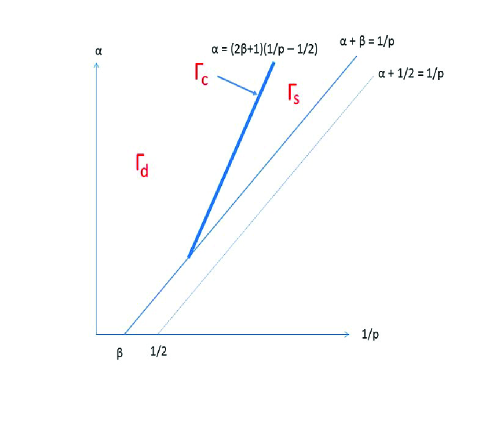
Figure 1: Different regimes ($\Gamma_{d}$: “dense”; $\Gamma_{s}$: “sparse”; $\Gamma_{c}$: “critical”) for the rate of convergence when $0\leq\beta\leq 1/2$.

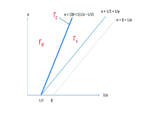
Figure 2: Different regimes ($\Gamma_{d}$: “dense”; $\Gamma_{s}$: “sparse”; $\Gamma_{c}$: “critical”) for the rate of convergence when $\beta>1/2$.

Theorem 3.1.

Assume observation model (5) with $\epsilon_{j}=\epsilon 2^{\beta j},\beta\geq 0$. Suppose that $\alpha>(1/p-1/2)_{+}$ for all $p$, and $\alpha+\beta>1/p$ for $0<p<2$. Define the rate exponent

$$r=\begin{cases}\frac{2\alpha}{2\alpha+2\beta+1}&\boldsymbol{\gamma}\in\Gamma_{d}\\ \frac{2\alpha-2/p+1}{2\alpha+2\beta-2/p+1}&\boldsymbol{\gamma}\in\Gamma_{s}\\ 1-p/2&\boldsymbol{\gamma}\in\Gamma_{c}.\end{cases}$$ (17)

Then, for $0<\epsilon<\epsilon_{0}$ ($\epsilon_{0}$ may depend on $C$), we have

$$\inf_{\widehat{\theta}}\sup_{\theta\in\Theta_{p,q}^{\alpha}(C)}\mathbb{E}\parallel\widehat{\theta}-\theta\parallel^{2}~{}\asymp~{}\begin{cases}C^{2(1-r)}\epsilon^{2r}&\boldsymbol{\gamma}\in\Gamma_{d}\\ C^{2(1-r)}\epsilon^{2r}(1+\log(C/\epsilon))^{r}&\boldsymbol{\gamma}\in\Gamma_{s}\\ C^{2(1-r)}\epsilon^{2r}(1+\log(C/\epsilon))^{r+(1-p/q)_{+}}&\boldsymbol{\gamma}\in\Gamma_{c}\end{cases}$$ (18)

where “$\asymp$” means that both sides are within positive constant multiples of each other, where the constants depend on $\alpha$, $\beta$, $p$, $\zeta$, $\Xi_{0}$ and $\Xi_{1}$. Moreover, the optimal rates are attained by the estimator defined through (15) and (16).

Remark 3.1.

We can expand the domain of applicability of Theorem 3.1 to $\{\boldsymbol{\gamma}:\alpha+\beta>1/p-1/2+1/(2K)\}$ where $K>1$, when $0<p<2$, if we also have $\alpha>1/p-1/2$. However, this requires modifying the expression of $j_{\epsilon}$ in (16) to $K\log_{2}\epsilon^{-2}$.

4 Upper bound on the risk

This section outlines the approach to establishing the upper bounds in Theorem 3.1.

Oracle inequalities at a single resolution level.  As a first step towards deriving upper bounds on the risk of $\widehat{\theta}=(\widehat{\theta}_{j})_{j\geq j_{0}}$, with $\widehat{\theta}_{j}$ defined by (15), we bound the risk of the estimator defined by (12) through the “oracle inequalities” that bound the maximal empirical complexity in terms of the maximal theoretical complexity plus an asymptotically small term.

With a slight abuse of notation, we write $L_{J}$ for $L_{n,n_{J}}$, where $J\subset\{1,\ldots,n\}$ and $n_{J}=|J|$. Then define

$$M_{n}^{\prime}=\sum_{J\neq\{\}}e^{-L_{J}n_{J}},$$ (19)

where the sum is taken over all subsets $J$ of $\{1,\ldots,n\}$. As long as $\nu_{n}>e^{1/(1+2\beta)}$, we have,

$$M_{n}^{\prime}\leq C_{\beta}n^{-2\beta}\nu_{n}^{-1},$$ (20)

for some $C_{\beta}>0$, as is shown in SM.

For any $\theta\in\mathbb{R}^{n}$, let $\theta_{J}=P_{J}\theta$, where $(P_{J}y)_{i}=y_{i}$ if $i\in J$, and $(P_{J}y)_{i}=0$, if $i\not\in J$. Now, let $\widehat{\theta}_{J}=P_{J}y$. Then, define the complexity criterion

$$C_{\epsilon}(J,y)=\parallel y-\widehat{\theta}_{J}\parallel^{2}+\epsilon^{2}\mbox{pen}(n_{J})=\sum_{i\not\in J}y_{i}^{2}+\epsilon^{2}\mbox{pen}(n_{J}).$$ (21)

Define

$$\widehat{J}=\arg\min_{J\subset\{1,\ldots,n\}}C_{\epsilon}(J,y)$$ (22)

and observe that, $\widehat{\theta}=P_{\widehat{J}}y=\widehat{\theta}_{\widehat{J}}$. Moreover, if we define

$${\cal R}(\theta,\epsilon):=\inf_{\theta^{\prime}}\parallel\theta-\theta^{\prime}\parallel^{2}+\epsilon^{2}\mbox{pen}(N(\theta^{\prime})),$$ (23)

then $\min_{J}C_{\epsilon}(J,\theta)={\cal R}(\theta,\epsilon)$.

The next step is the following non-asymptotic bound on the risk of the penalized least squares estimator (9) which is especially useful for dealing with our problem. This a restatement of Theorem 11.9 of Johnstone (2013).

Proposition 4.1.

Let $\widehat{\theta}$ be the penalized least squares estimator of (9) and (12) for the penalty (10) and with $M_{n}^{\prime}$ defined by (19). Then there exists a constant $D=D(\zeta)$ such that

$$\mathbb{E}\parallel\widehat{\theta}-\theta\parallel^{2}\leq D\left[2M_{n}^{\prime}\xi_{1}\epsilon^{2}+\min_{J}C_{\epsilon}(J,\theta)\right]=D\left[2M_{n}^{\prime}\xi_{1}\epsilon^{2}+{\cal R}(\theta,\epsilon)\right].$$ (24)

The constant $D$ may be taken to be $2\zeta(\zeta+1)^{3}(\zeta-1)^{-3}$.

We will need to bound the ‘ideal risk’ $\mathcal{R}(\theta,\epsilon)$ over certain $\ell_{p}$ balls $\ell_{n,p}(C)=\{x\in\mathbb{R}^{n}:\sum_{i=1}^{n}|x_{i}|^{p}\leq C^{p}\}$. To state the bound, we introduce control functions $r_{n,p}(C)$. For $C>0$ and $0<p<2$, let

$$r_{n,p}(C)=\begin{cases}C^{2}&~{}\mbox{if}~{}~{}C\leq\sqrt{1+\log n},\\ C^{p}[1+\log(n/C^{p})]^{1-p/2}&~{}\mbox{if}~{}~{}\sqrt{1+\log n}\leq C\leq n^{1/p},\\ n&~{}\mbox{if}~{}~{}C\geq n^{1/p},\\ \end{cases}$$ (25)

while for $p\geq 2$, let

$$r_{n,p}(C)=\begin{cases}n^{1-2/p}C^{2}&~{}\mbox{if}~{}~{}C\leq n^{1/p},\\ n&~{}\mbox{if}~{}~{}C\geq n^{1/p}.\\ \end{cases}$$ (26)

When $p<2$, we shall refer to the region $C\geq n^{1/p}$ as the “dense zone”, the region $\sqrt{1+\log n}\leq C\leq n^{1/p}$ as the “sparse zone” and the region $C\leq\sqrt{1+\log n}$ as the “highly sparse zone”. When $p\geq 2$, we shall refer to the region $C\geq n^{1/p}$ as the “large signal zone” and the region $C\leq n^{1/p}$ as the “small signal zone”.

The proof of the next bound is given in SM.

Lemma 4.1.

For the ‘ideal risk’ defined in (9)- (11), there exists $c>0$ such that

$$\sup_{\theta\in\ell_{n,p}(C)}\mathcal{R}(\theta,\epsilon)\leq c(\log\nu)\epsilon^{2}r_{n,p}(C/\epsilon).$$ (27)

A general MSE bound.  Now we establish a general purpose upper bound for the risk of the estimator $\widehat{\theta}$ when $\theta\in\Theta_{p,q}^{\alpha}(C)$. Let

$$T(\theta,\epsilon)=\mathbb{E}_{\theta}\parallel\widehat{\theta}-\theta\parallel^{2}=\sum_{j\geq j_{0}}\mathbb{E}_{\theta}\parallel\widehat{\theta}_{j}-\theta_{j}\parallel^{2}.$$

By Proposition 4.1 we have the following bound:

$$T(\theta,\epsilon)/D\leq 2\sum_{j\geq j_{0}}\xi_{j}M_{j}^{\prime}\epsilon_{j}^{2}+\sum_{j\geq j_{0}}{\cal R}_{j}(\theta_{j},\epsilon_{j})=:T_{1}(\epsilon)+T_{2}(\theta,\epsilon),$$ (28)

say, where $M_{j}^{\prime}$ is the analog of $M_{n}^{\prime}$ (defined in (19)) when $n$ is replaced by $n_{j}$, $\xi_{1}$ by $\xi_{j}$, $\nu$ by $\nu_{n_{j}}$, and

$${\cal R}_{j}(\theta_{j},\epsilon_{j}):=\min_{\theta_{j}^{\prime}}\parallel\theta_{j}^{\prime}-\theta_{j}\parallel^{2}+\epsilon_{j}^{2}\mbox{pen}(N(\theta_{j}^{\prime}))$$

is the theoretical complexity in level $j$, and $D>0$ is some constant. The bound (20) is constructed to offset the geometric growth of $\epsilon_{j}^{2}=2^{2\beta j}\epsilon^{2}$ and together with the choice (16) of $\nu_{n_{j}}$, we obtain the bound

$$T_{1}(\epsilon)\leq c(\zeta,\Xi_{1},\beta,\nu)\epsilon^{2}\log\epsilon^{-2},$$ (29)

which shows that this term is asymptotically negligible.

In order to deal with $T_{2}(\theta,\epsilon)$, first observe that with $a=\alpha+1/2-1/p$,

$$\theta\in\Theta_{p,q}^{\alpha}(C)\quad\Longrightarrow\quad\|\theta_{j}\|_{p}\leq C_{j}:=C2^{-aj},\qquad\forall~{}j\geq 1.$$ (30)

We bound $T_{2}(\theta,\epsilon)$ by using bounds for the theoretical complexities $\mathcal{R}_{j}(\theta_{j},\epsilon_{j})$ over the corresponding Besov shells. Indeed, with $R_{j}:=\epsilon_{j}^{2}r_{n_{j},p}(C_{j}/\epsilon_{j})$, from (27) we have

$$\sup_{\theta\in\Theta_{p,q}^{\alpha}(C)}T_{2}(\theta,\epsilon)=\sup_{\theta\in\Theta_{p,q}^{\alpha}(C)}\sum_{j\geq j_{0}}{\cal R}_{j}(\theta_{j},\epsilon_{j})\leq c\sum_{j\geq j_{0}}(\log\nu_{n,j})R_{j}.$$ (31)

“Dense” regime:  Here, $\alpha>(2\beta+1)(1/p-1/2)_{+}$ and so $r=2\alpha/(2\alpha+2\beta+1)$. We show that for $p\geq 2$, there exists an index $j_{*}$—which we allow to be real valued—such that $R_{j}$ reaches its peak $R_{*}=R_{j_{*}}$ at $j=j_{*}$ and decays geometrically away from it. Specifically, we show that

$$R_{*}=C^{2(1-r)}\epsilon^{2r}.$$ (32)

The index $j_{*}$ is determined by solving the equation $C_{j_{*}}=\epsilon_{j_{*}}n_{j_{*}}^{1/p}$, i.e., at the “large signal – small signal” boundary (see (26)). Note that this equation reduces to

$$2^{(\alpha+\beta+1/2)j_{*}}=(C/\epsilon).$$ (33)

We also show that, for $p\geq 2$,

$$R_{j}=\begin{cases}R_{*}2^{(2\beta+1)(j-j_{*})}&~{}\mbox{if}~{}j\leq j_{*}\\ R_{*}2^{-2\alpha(j-j_{*})}&~{}\mbox{if}~{}j\geq j_{*}.\\ \end{cases}$$ (34)

For $0<p<2$, we have an additional index $j_{+}>j_{*}$ which is obtained from the equation $C_{j_{+}}=\epsilon_{j_{+}}(1+\log n_{j_{+}})^{1/2}$, i.e., at the “sparse – highly sparse zone” boundary (see (25)). Thus, $j_{+}$ satisfies

$$2^{(\alpha+\beta-1/p+1/2)j_{+}}(1+\log n_{j_{+}})^{1/2}=(C/\epsilon).$$ (35)

In this case, there is a second peak of $R_{j}$ at $j=j_{+}$. Defining $R_{+}=R_{j_{+}}$, from (25), we deduce that $R_{+}=C^{2}2^{-2aj_{+}}$. We also show that when $p<2$,

$$R_{j}=\begin{cases}R_{*}2^{(2\beta+1)(j-j_{*})}&~{}\mbox{if}~{}j<j_{*}\\ R_{*}2^{-p\rho(j-j_{*})}[1+\varphi(j-j_{*})]^{1-p/2}&~{}\mbox{if}~{}j_{*}\leq j<j_{+}\\ R_{+}2^{-2a(j-j_{+})}&~{}\mbox{if}~{}j\geq j_{+},\\ \end{cases}$$ (36)

where $\rho:=\alpha-(2\beta+1)(1/p-1/2)>0$ and $\varphi=p(\alpha+\beta+1/2)\log 2$. The schematic behavior of the shell risk is depicted in Figure 3. In particular, using (33), (35) and (40) (stated below), it can be checked that $R_{*}\geq R_{+}$ for small enough $\epsilon$. The proofs of (32) and (36) are as in Section 12.5 of Johnstone (2013), and hence are given in SM. From (35), we deduce that

$$j_{+}=\delta^{-1}\log_{2}(C/\epsilon)(1+o(1))~{}~{}~{}\mbox{as}~{}\epsilon\to 0,~{}~{}~{}\mbox{where}~{}~{}\delta:=\alpha+\beta-1/p+1/2.$$ (37)

Since $\alpha+\beta>1/p$, so that $\delta>1/2$, we have $j_{+}<j_{\epsilon}$ for $0<\epsilon<\epsilon_{0}(C)$ (compare with Remark 3.1). Thus, by the geometric decay of $R_{j}$ for $j\geq j_{+}$, and (16) and (31), the risk upper bound follows in the setting $0<p<2$. When $p\geq 2$, by (33) we have $j_{*}<j_{\epsilon}$, and so a similar argument, now involving (34), establishes the risk upper bound.

“Sparse” regime:  Now, we consider the setting where $0<p<2$, $\alpha<(2\beta+1)(1/p-1/2)$ and $\alpha+\beta>1/p$. The basic strategy is similar to that in the dense case, namely, bounding $R_{j}$ by splitting the scale indices $j$’s into three parts: $j\leq j_{*}$, $j_{*}<j<j_{+}$ and $j\geq j_{+}$, respectively. Since $R_{j_{+}}=C^{2}2^{-2aj_{+}}$, noticing that $r=a/\delta$, by (33), we have

$$R_{+}=R_{j_{+}}=C^{2}2^{-2aj_{+}}=C^{2}\left(\frac{C^{2}}{\epsilon^{2}}\right)^{-r}(1+\log n_{j_{+}})^{r}\asymp C^{2(1-r)}\epsilon^{2r}(1+\log(C/\epsilon))^{r}$$ (38)

as $\epsilon\to 0$, where the last step follows from (37).

For $j\not\in[j_{*},j_{+})$, the equalities in (36) remain valid, while it is shown in SM that

$$R_{j}\leq R_{+}2^{-\tau(j_{+}-j)}~{}~{}\mbox{for}~{}j_{*}\leq j<j_{+},$$ (39)

where $\tau=(2\beta+1)-p(\alpha+\beta+1/2)=-p[\alpha-(2\beta+1)(1/p-1/2)]=-p\rho>0$.

Observe that

$$\frac{\alpha}{\alpha+\beta+1/2}\geq\frac{\alpha-1/p+1/2}{\alpha+\beta-1/p+1/2}~{}~{}\Leftrightarrow~{}~{}\alpha\leq(2\beta+1)\left(\frac{1}{p}-\frac{1}{2}\right),$$ (40)

while equality on one side implies equality on the other. Defining $r^{\prime}=\alpha/(\alpha+\beta+1/2)$, by (33),

$$R_{*}=R_{j_{*}}=n_{j_{*}}\epsilon_{j_{*}}^{2}=\epsilon^{2}2^{(2\beta+1)j_{*}}=\epsilon^{2}\left(\frac{C^{2}}{\epsilon^{2}}\right)^{1-r^{\prime}}=C^{2}\left(\frac{C^{2}}{\epsilon^{2}}\right)^{-r^{\prime}}.$$ (41)

Thus, recalling (38), from (40) we conclude that $R_{j_{*}}\leq R_{j_{+}}$. Combining, we obtain the result. Again, since $j_{+}<j_{\epsilon}$ for $0<\epsilon<\epsilon_{0}(C)$, by (16) and (31), the risk upper bound follows.

The proof of the rate upper bound in the “critical” regime is given in SM.

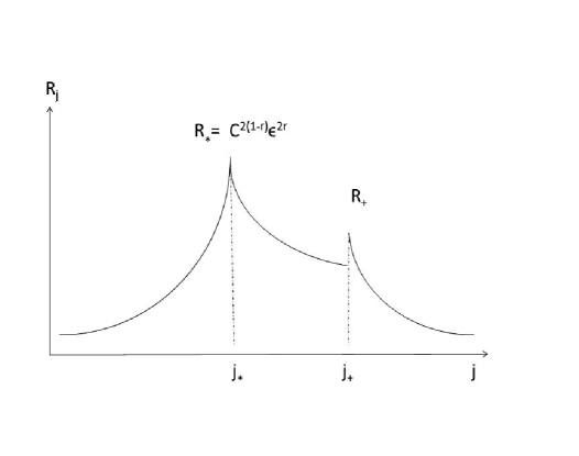
Figure 3: Schematic behavior of “shell risk” $R_{j}$, with $j$ treated as a real variable.

5 Lower bound on the risk

The idea for the risk lower bound is to minorize the minimax risk of the model (5) by the minimax risk of a i.i.d. Gaussian noise model with covaraince matrix $\Xi_{0}I$. Then a lower bound on the latter is obtained by considering a restricted parameter space for $\theta$ such that all the level-wise components $\theta_{j}$ are 0 except for certain specific dyadic levels $j$, and in those levels the vectors $\theta_{j}$ are restricted to lie in $\ell_{p}$ balls of appropriate radii. Thereafter we can use minimax risk asymptotics for $\ell_{p}$ balls Johnstone (2013) to show that the lower bound thus obtained is of the right asymptotic order.

Equivalence to white noise.  We first show that the minimax risk with noise $z_{jk}$ in the model (5) can be bounded below by the minimax risk from a white noise model. Indeed, let $\Xi_{0}$ and $\Xi_{1}$ be as in (4). Then we define a new model

$$\tilde{y}_{jk}=\theta_{jk}+\Xi_{0}\epsilon_{j}w_{jk},\qquad k=1,\ldots,2^{j},\quad j\geq j_{0},$$ (42)

where $w_{jk}$ are i.i.d. $N(0,1)$. We denote the minimax risk for estimating $(\theta)$ in $\ell_{2}$ loss and with scale parameter $\epsilon$ in model (5) by $R_{z}(\Theta_{p,q}^{\alpha}(C),\epsilon):=\inf_{\widehat{\theta}}\sup_{\theta\in\Theta_{p,q}^{\alpha}(C)}\parallel\widehat{\theta}-\theta\parallel_{2}^{2}$, and that in model (42) by $R_{w}(\Theta_{p,q}^{\alpha}(C),\Xi_{0}\epsilon)$. Then, using Lemma 4.28 of Johnstone (2013), we conclude that

$$R_{z}(\Theta_{p,q}^{\alpha}(C),\epsilon)\geq R_{w}(\Theta_{p,q}^{\alpha}(C),\Xi_{0}\epsilon).$$ (43)

Thus, it suffices to provide lower bounds on the latter quantity that match with the bounds in Theorem 3.1. In the next subsection, we give an outline of the rate lower bound in the “dense” and “sparse” regimes.

Lower bound : “dense” and “sparse” regimes.  In both the “dense” and “sparse” regimes, our strategy is to consider restricted parameter spaces that are Besov-shells $\Theta^{(j)}(C):=\{\theta:\parallel\theta_{j}\parallel_{p}\leq C_{j}~{}\mbox{and}~{}\theta_{j^{\prime}}=0~{}\mbox{if}~{}j^{\prime}\neq j\}$, for appropriately chosen $j$. Then, $\Theta^{(j)}(C)$ is isomorphic to the $\ell_{p}$ ball $\ell_{n_{j},p}(C_{j})$. Let $R_{w}(\Theta^{(j)},\Xi_{0}\epsilon)$ denote the minimax risk over $\Theta^{(j)}$, and let $R_{N}(\ell_{n_{j},p}(C_{j}),\Xi_{0}\epsilon_{j})$ denote the minimax risk (for estimating $\theta_{j}$) over the parameter space $\ell_{n_{j},p}(C_{j})$, both with respect to the $\ell_{2}$-loss. Since $\Theta^{(j)}(C)\subset\Theta_{p,q}^{\alpha}(C)$, and the $\ell_{2}$ loss is coordinate-wise additive, we have

$$R_{w}(\Theta_{p,q}^{\alpha}(C),\Xi_{0}\epsilon)\geq R_{w}(\Theta^{(j)}(C),\Xi_{0}\epsilon)\geq R_{N}(\ell_{n_{j},p}(C_{j}),\Xi_{0}\epsilon_{j}).$$ (44)

We treat the “dense” regime first. Consider the Besov shell $\Theta^{(j_{*})}(C)$, where $j_{*}$ is defined by (33) (treating $j_{*}$ as an integer, for simplicity). Then it follows from Theorem 13.16 of Johnstone (2013) (restated as Theorem S1 in SM) that

$$R_{N}(\ell_{n_{j},p}(C_{j_{*}}),\Xi_{0}\epsilon_{j_{*}})\geq c\Xi_{0}^{2}\epsilon_{j_{*}}^{2}n_{j_{*}}$$ (45)

for some $c>0$, for small enough $\epsilon$. Invoking (33), we conclude from (43), (44) and (45) that, for some $c^{\prime}>0$,

$$R_{z}(\Theta_{p,q}^{\alpha}(C),\epsilon)\geq c^{\prime}C^{2(1-r)}\epsilon^{2r},$$

where $r=2\alpha/(2\alpha+2\beta+1)$.

In the “sparse” regime, we consider the Besov-shell $\Theta^{(j_{+})}(C)$ where $j_{+}$ is defined in (35). Then, by part (b) of Theorem 13.16 of Johnstone (2013), we obtain that

$$R_{N}(\ell_{n_{j},p}(C_{j_{+}}),\Xi_{0}\epsilon_{j_{+}})\geq c\Xi_{0}^{2}\epsilon_{j_{+}}^{2}\log n_{j_{+}}$$ (46)

for some $c>0$ and for small enough $\epsilon$. Using (35) and (37), from (43), (44) and (46), we conclude that for some $c^{\prime}>0$,

$$R_{z}(\Theta_{p,q}^{\alpha}(C),\epsilon)\geq c^{\prime}C^{2(1-r)}\epsilon^{2r}(1+\log(C/\epsilon))^{r},$$ (47)

where $r=(2\alpha-2/p+1)/(2\alpha+2\beta-2/p+1)$.

Proof of the lower bound in the “critical” regime is given in SM.

Acknowledgement

The authors thank Laurent Cavalier for helpful discussions whose untimely death is deeply regretted. Johnstone’s research is partially supported by NSF grant DMS 0906812, Paul’s research is partially supported by NSF grants DMR 1035468 and DMS 1106690.

Supplementary Material

Proof of equation (20):

Using the Stirling’s formula bound $k!>\sqrt{2\pi k}k^{k}e^{-k}$,

$$M^{\prime}\leq\sum_{k=1}^{n}\frac{n^{k}}{k!}\left(\frac{k}{n\nu}\right)^{k(1+2\beta)} \leq \sum_{k=1}^{\infty}\frac{1}{\sqrt{2\pi k}}\left(\frac{k^{2\beta}}{n^{2\beta}}\frac{e}{\nu^{1+2\beta}}\right)^{k}$$

$$\leq \frac{1}{n^{2\beta}\nu}\sum_{k=1}^{\infty}\frac{k^{2\beta}e}{\sqrt{2\pi k}}\left(\frac{e}{\nu^{1+2\beta}}\right)^{k-1}\leq\frac{C_{\beta}}{n^{2\beta}\nu}$$

where, in the last step we used the fact that $\nu>e^{1/(1+2\beta)}$.

Proof of Lemma 4.1:

Let $|\theta_{(1)}|\geq\cdots\geq|\theta_{(n)}|$ be a decreasing rearrangement of $\theta$. Then, it is easy to see that

$${\cal R}(\theta,\epsilon)\leq\sum_{k=1}^{n}\theta_{(k)}^{2}\wedge\epsilon^{2}\lambda_{k}^{2}=\epsilon^{2}\sum_{k=1}^{n}(\theta_{(k)}/\epsilon)^{2}\wedge\lambda_{n,k}^{2},$$ (S1)

where $\lambda_{n,k}=\sqrt{\xi_{1}\zeta}(1+\sqrt{2(1+2\beta)\log(\nu n/k)})$.

First, consider the case $p\geq 2$. Setting $k=n$ in (S1) and noticing that $\lambda_{n,n}^{2}\leq c\log\nu$ for some $c>0$, we have

$${\cal R}(\theta,\epsilon)\leq c(\log\nu)\epsilon^{2}n.$$ (S2)

This bound is valid for all values of $C>0$ and actually for all values of $p>0$. Moreover, this bound is dominant in particular in the “dense zone”: $C/\epsilon\geq n^{1/p}\sqrt{\log\nu}$, in which case the bound reduces to the form $c(\log\nu)\epsilon^{2}r_{n,p}(C/\epsilon)$. Next, by setting $k=0$ in (S1), we have

$${\cal R}(\theta,\epsilon)\leq n\epsilon^{2}(n^{-1}\sum_{k=1}^{n}|\theta_{k}/\epsilon|^{2})\leq n\epsilon^{2}(n^{-1}\sum_{k=1}^{n}|\theta_{k}/\epsilon|^{p})^{2/p}\leq\epsilon^{2}n^{1-2/p}(C/\epsilon)^{2}=\epsilon^{2}r_{n,p}(C/\epsilon).$$

Clearly, the latter is bounded by $c(\log\nu)n^{1-p/2}C^{2}$ which dominates when $0<C/\epsilon<n^{1/p}$.

For $p<2$, we first notice that since $\theta\in\ell_{n,p}(C)$, it implies that $|\theta_{(k)}|\leq Ck^{-1/p}$ for $k=1,\ldots,n$. Therefore, we obtain for all $k\geq 0$,

$$\sum_{j>k}\theta_{(j)}^{2}\leq C^{2-p}(k+1)^{1-2/p}\sum_{j>k}|\theta_{(j)}|^{p}\leq C^{2}(k+1)^{1-2/p}.$$

Now, invoking this in (S1) and setting $k=0$, we have

$${\cal R}(\theta,\epsilon)\leq\epsilon^{2}(C/\epsilon)^{2}$$

which is clearly bounded by $(\log\nu)C^{2}$, and the latter is of the form $c(\log\nu)\epsilon^{2}r_{n,p}(C/\epsilon)$ in the “sparse zone”: $C\leq\sqrt{1+\log n}$. For the “dense zone”: $C\geq n^{1/p}$, we can use the universal bound (i.e., valid for all $p>0$) given by (S2) and we observe that it is also of the form $c(\log\nu)\epsilon^{2}r_{n,p}(C/\epsilon)$. Thus, it only remains to prove the bound (27) in the case $0<p<2$ and $\sqrt{1+\log n}\leq C\leq n^{1/p}$. The proof of this follows by using an optimization argument as in Section 11.4 of Johnstone (2013) and is omitted.

Proof of equations (32) and (34) :

To prove (32), observe that by (26),

$$R_{*}=R_{j_{*}} = n_{j_{*}}\epsilon_{j_{*}}^{2}~{}=~{}\epsilon^{2}2^{(2\beta+1)j_{*}}~{}=~{}C^{2}2^{-2\alpha j_{*}}\qquad(\mbox{by}~{}(\ref{eq:j_star_expand}))$$ (S3)

$$= C^{2}\left(2^{2(\alpha+\beta+1/2)j_{*}}\right)^{-r}=C^{2(1-r)}\epsilon^{2r}.$$

Moreover, we have

$$\log_{2}(R_{+}/R_{*})=2(\alpha j_{*}-aj_{+})$$ (S4)

which follows from the first line of (S3) and the expression for $R_{+}$. From this and (33) and (35), and using $\rho>0$, it can be deduced that $R_{+}\leq R_{*}$, which ensures that the final bound on $\sup_{\theta\in\Theta_{p,q}^{\alpha}(C)}T_{2}(\theta,\epsilon)$ is $O(R_{*})$.

For the rest of the proof, we note that $C_{j}/\epsilon_{j}$ is a monotonically decreasing sequence in $j$. We first show that (34) holds when $p\geq 2$. First, if $j\leq j_{*}$, then we are in the “large signal zone”, i.e., $C_{j}/\epsilon_{j}\geq n_{j}^{1/p}$. Hence, $R_{j}=n_{j}\epsilon_{j}^{2}=\epsilon^{2}2^{(2\beta+1)j}$. Hence, the result holds by the first line of (S3). Now, if $j>j_{*}$, then we are in the in the “small signal zone”, i.e., $C_{j}/\epsilon_{j}<n_{j}^{1/p}$ so that $R_{j}=n_{j}^{1-p/2}C_{j}^{2}$, from which the result follows by (33) and (S3).

Proof of equation (36):

When $p<2$, we first note that the first bound (i.e., when $j\leq j_{*}$), and its proof are exactly the same as in the case $p\geq 2$. The case $j\geq j_{+}$ corresponds to “highly sparse zone”, i.e., $C_{j}/\epsilon_{j}\leq(1+\log n_{j})^{1/2}$, and hence we have $R_{j}=C_{j}^{2}=C^{2}2^{-2aj}$, which shows, by comparing with $R_{+}$, that the result holds in this case. Finally, we turn to the setting $j_{*}\leq j<j_{+}$, i.e., the “sparse zone”. In this case, define $\eta_{j}=(C_{j}/\epsilon_{j})n_{j}^{-1/p}$. Then,

$$R_{j}=C_{j}^{p}\epsilon_{j}^{2-p}(1+\log(n_{j}\epsilon_{j}^{p}/C_{j}^{p}))^{1-p/2}=n_{j}\epsilon_{j}^{2}\eta_{j}^{p}(1+\log\eta_{j}^{-p})^{1-p/2}.$$ (S5)

Thus,

$$\eta_{j}^{-p}=2^{p(\alpha+\beta+1/2)(j-j_{*})}\left[2^{(\alpha+\beta+1/2)j_{*}}/(C/\epsilon)\right]^{p}=2^{p(\alpha+\beta+1/2)(j-j_{*})},$$ (S6)

where the second equality is by (33). Hence, from (S5) and the fact that $R_{*}=R_{j_{*}}=n_{j_{*}}\epsilon_{j_{*}}^{2}$, the result follows.

Verification of equation (39) :

By (S5) and (S6), and recalling that $\tau=(2\beta+1)-p(\alpha+\beta+1/2)$, we have

$$R_{j} = \epsilon^{2}\left(\frac{C}{\epsilon}\right)^{p}2^{[(2\beta+1)-p(\alpha+\beta+1/2)]j}(1+\log\eta_{j}^{-p})^{1-p/2}$$

$$= \epsilon^{2}2^{p[(\alpha+\beta-1/p+1/2)-\alpha+(2\beta+1)(1/p-1/2)]j_{+}}(1+\log n_{j_{+}})^{p/2}(1+\log\eta_{j}^{-p})^{1-p/2}2^{-\tau(j_{+}-j)}$$

$$= \epsilon^{2}2^{2\beta j_{+}}(1+\log n_{j_{+}})^{p/2}(1+\log\eta_{j}^{-p})^{1-p/2}2^{-\tau(j_{+}-j)}$$

$$= \epsilon^{2}\left(\frac{C^{2}}{\epsilon^{2}}\right)^{1-r}(1+\log n_{j_{+}})^{r-(1-p/2)}(1+\log\eta_{j}^{-p})^{1-p/2}2^{-\tau(j_{+}-j)}$$

$$\leq C^{2(1-r)}\epsilon^{2r}(1+\log n_{j_{+}})^{r}2^{-\tau(j_{+}-j)}$$

$$= R_{+}2^{-\tau(j_{+}-j)},$$

where the second and fourth equalities are due to (35) and the inequality follows from the fact that $\eta_{j}$’s are decreasing and that $n_{j_{+}}\eta_{j_{+}}^{p}=(C_{j_{+}}/\epsilon_{j_{+}})^{p}\geq 1$ (since $C_{j_{+}}=\epsilon_{j_{+}}(1+\log n_{j_{+}})^{1/2}$), while the last equality is due to (38).

Proof of upper bound in the “critical” regime

Here, $\alpha=(2\beta+1)(1/p-1/2)$ and $0<p<2$. We again consider three separate blocks : $j\leq j_{*}$, $j_{*}<j<j_{+}$ and $j\geq j_{+}$. The treatment of the first and the last block of indices is the same as in the “sparse” case above. So, we focus on the middle block.

The conditions $\theta\in\Theta_{p,q}^{\alpha}(C)$ and $\alpha=(2\beta+1)(1/p-1/2)$ imply that $\alpha-1/p+1/2=2\beta(1/p-1/2)$ so that

$$\sum_{j=j_{*}}^{j_{+}}2^{2\beta(1/p-1/2)qj}\parallel\theta_{j}\parallel_{p}^{q} \leq C^{q}~{}~{}~{}\Rightarrow~{}~{}~{}\sum_{j=j_{*}}^{j_{+}}2^{(2\beta q/p)j}\parallel\mu_{j}\parallel_{p}^{q}~{}\leq~{}\left(\frac{C}{\epsilon}\right)^{q},$$ (S7)

where $\mu_{j}=(\mu_{jk})_{k=1}^{n_{j}}$ and $\mu_{jk}:=\epsilon_{j}^{-1}\theta_{jk}$. In the following, instead of using the omnibus bound (31) on $T_{2}(\theta,\epsilon)$ we use the more direct bound ${\cal R}_{j}(\theta_{j},\epsilon_{j})\leq c(\log\nu_{n,j})\epsilon_{j}^{2}r_{n_{j},p}(\parallel\mu_{j}\parallel_{p})$ (for some constant $c>0$ independent of the parameters $\theta$, $C$ and $\epsilon$), and then, noticing that $j_{+}<j_{\epsilon}$ so that $\log\nu_{n,j}=\log\nu$, maximize the sum $\sum_{j=j_{*}}^{j_{+}}\epsilon_{j}^{2}r_{n_{j},p}(\parallel\mu_{j}\parallel_{p})$ subject to (S7).

In view of (S7), since $j\geq j_{*}$, from the fact that $C_{j_{*}}=\epsilon_{j_{*}}n_{j_{*}}^{1/p}$ so that $C/\epsilon=2^{(\alpha+\beta+1/2)j_{*}}$, we obtain

$$\parallel\mu_{j}\parallel_{p}\leq(C/\epsilon)2^{-(2\beta/p)j}\leq 2^{(\alpha+\beta+1/2)j}2^{-(2\beta/p)j}=2^{j/p}=n_{j}^{1/p}.$$

Thus, from (25), for $j_{*}\leq j\leq j_{+}$,

$$r_{n_{j},p}(\parallel\mu_{j}\parallel_{p}) \leq c\max\{\parallel\mu_{j}\parallel_{p}^{p}(1+\log(n_{j}/\parallel\mu_{j}\parallel_{p}^{p}))^{1-p/2},\parallel\mu_{j}\parallel_{p}^{2}\}~{}\leq~{}\parallel\mu_{j}\parallel_{p}^{p}(1+\log n_{j})^{1-p/2},$$ (S8)

where the second inequality follows by noticing that the bound $\parallel\mu_{j}\parallel_{p}^{2}$ holds only in the “highly sparse zone”: $\parallel\mu_{j}\parallel_{p}\leq(1+\log n_{j})^{1/2}$. Thus, we consider a majorizing bound for $\sum_{j=j_{*}}^{j_{+}}{\cal R}_{j}(\theta_{j},\epsilon)$ by maximizing

$$\epsilon^{2}(1+\log n_{j_{+}})^{1-p/2}\sum_{j=j_{*}}^{j_{+}}2^{2\beta j}\parallel\mu_{j}\parallel_{p}^{p}~{}~{}~{}\mbox{subject to}~{}(\ref{eq:crit_constr}).$$

Set $x_{j}=2^{2\beta j}\parallel\mu_{j}\parallel_{p}^{p}$, define $x=(x_{j})_{j=j_{*}}^{j_{+}}$, and then the optimization problem reduces to

$$\mbox{maximize}~{}~{}~{}\epsilon^{2}(1+\log n_{j_{+}})^{1-p/2}\parallel x\parallel_{1}\qquad\mbox{subject to}\qquad\parallel x\parallel_{q/p}\leq(C/\epsilon)^{p}.$$

The value of this maximum is $\epsilon^{2}(1+\log n_{j_{+}})^{1-p/2}(j_{+}-j_{*})^{(1-p/q)_{+}}(C/\epsilon)^{p}$. Now, invoking (33) and (35), we get $j_{+}-j_{*}<p[2\beta(2\beta+1)]^{-1}\log_{2}(C/\epsilon)$, and consequently,

$$\sum_{j=j_{*}}^{j_{+}}{\cal R}_{j}(\theta_{j},\epsilon)\leq c\epsilon^{2}(C/\epsilon)^{p}(1+\log(C/\epsilon))^{(1-p/2)+(1-p/q)_{+}}.$$ (S9)

Notice that since $\alpha=(2\beta+1)(1/p-1/2)$, we have

$$r=1-p/2=\frac{\alpha-1/p+1/2}{\alpha+\beta-1/p+1/2}=\frac{\alpha}{\alpha+\beta+1}=r^{\prime},$$

so that from (41) and (38), we have $R_{j_{*}}\leq R_{j_{+}}$, and the latter is dominated by the upper bound in (S9). Thus, the upper bound for $T_{2}(\theta,\epsilon)$ in the critical case follows by combining with the bounds on $R_{j}$ for $j\leq j_{*}$ and $j\geq j_{+}$.

Details on equations (45) and (46)

Theorem 13.16 of Johnstone (2013), stated below, states the asymptotic behavior of the minimax risk of estimation of $\mu\in\mathbb{R}^{n}$, under the data model

$$y_{k}=\mu_{k}+\epsilon_{n}z_{k},\qquad k=1,\ldots,n,$$ (S10)

where $\epsilon_{n}>0$ and the random variables $z_{k}$ are i.i.d. $N(0,1)$. The minimax risk is calculated using the squared error loss and over the parameter space $\ell_{n,p}(C_{n})$, with $C_{n}>0$, i.e.,

$$R_{N}(\ell_{n,p}(C_{n}),\epsilon_{n})=\inf_{\widehat{\mu}}\sup_{\mu\in\ell_{n,p}(C_{n})}\parallel\widehat{\mu}-\mu\parallel_{2}^{2}.$$ (S11)

Johnstone (2013) derived the asymptotic expression for $R_{N}(\ell_{n,p}(C_{n}),\epsilon_{n})$, as $\epsilon_{n}\to 0$, by first deriving an expression for the Bayes minimax risk in the univariate (i.e., $n=1$) problem, under the class of univariate priors

$$\mathfrak{m}_{p}(\tau)=\{\pi(d\mu):\int|\mu|^{p}\pi(d\mu)\leq\tau^{p}\},$$

so that, with $y\sim N(\mu,\epsilon^{2})$, the Bayes minimax risk with respect to the class $\mathfrak{m}_{p}(\tau)$ is given by

$$\beta_{p}(\tau,\epsilon)=\inf_{\widehat{\mu}}\sup_{\pi\in\mathfrak{m}_{p}(\tau)}B(\widehat{\mu},\pi)$$

where $B(\widehat{\mu},\pi)$ denotes the Bayes risk of the estimator $\widehat{\mu}$ under the squared error loss, with respect to the prior $\pi$. Proposition 13.4 of Johnstone (2013) states the properties of $\beta_{p}(\tau,\epsilon)$, in particular that it is (1) increasing in $p$; (2) decreasing in $\epsilon$; (3) strictly increasing, concave and continuous in $\tau^{p}$; and (4) $\beta_{p}(\tau,\epsilon)=\epsilon^{2}\beta_{p}(\tau/\epsilon,1)$ and $\beta_{p}(a\tau,\epsilon)\leq a^{2}\beta_{p}(\tau,\epsilon)$ for all $a\geq 1$.

Furthermore, if we define $\beta_{p}(\eta)=\beta_{p}(\eta,1)$, then Theorem 13.7 of Johnstone (2013) states that, as $\eta\to 0$,

$$\beta_{p}(\eta)\sim\begin{cases}\eta^{2}&~{}\mbox{if}~{}2\leq p\leq\infty,\\ \eta^{p}(2\log\eta^{-p})^{1-p/2}&~{}\mbox{if}~{}0<p<2.\\ \end{cases}$$

Theorem 13.16 of Johnstone (2013), which summarizes the asymptotic behavior of $R_{N}(C_{n},\epsilon_{n})$, is stated in terms of the function $\beta_{p}(\eta)$.

Theorem S1.

(Theorem 13.16 of Johnstone (2013)): Introduce the normalized signal-to-noise ratios

$$\eta_{n}=n^{-1/p}(C_{n}/\epsilon_{n})\qquad\delta_{n}=(2\log n)^{-1/2}(C_{n}/\epsilon_{n}).$$ (S12)

For $2\leq p\leq\infty$, if $\eta_{n}\to\eta\in[0,\infty]$, then

$$R_{N}(C_{n},\epsilon_{n})\sim n\epsilon_{n}^{2}\beta_{p}(\eta_{n}).$$ (S13)

For $0<p<2$,

• if $\eta_{n}\to\eta\in[0,\infty]$ and $\delta_{n}\to\infty$ then again (S13) holds.

• If $\eta_{n}\to 0$ and $\delta_{n}\to\delta\in[0,\infty)$, then

  $$R_{N}(C_{n},\epsilon_{n})\sim\begin{cases}\lambda_{n}^{2}\epsilon_{n}^{2}([\delta]^{p}+\{\delta^{p}\}^{2/p}),&~{}\mbox{if}~{}\delta>0,\\ \lambda_{n}\epsilon_{n}^{2}\delta_{n}^{2},&~{}\mbox{if}~{}\delta=0,\\ \end{cases}$$ (S14)

  where $[\cdot]$ and $\{\cdot\}$ denote the integer and fractional parts, respectively, and $\lambda_{n}=\sqrt{2\log n}$.

We apply this result with $n=n_{j}$, $C_{n}=C_{j}$ and $\epsilon_{n}=\Xi_{0}\epsilon_{j}$, for $j=j_{*}$ in the “dense” case and for $j=j_{+}$ in the “sparse” case. It is easy to verify using (33), (35) and (35) that the conditions for Theorem S1 are satisfied and some elementary calculations then lead to (45) and (46).

Proof of lower bound in the “critical” regime

Next, we consider the “critical” regime. If $p/q\geq 1$, then the lower bound on the minimax risk for the “critical” regime is a continuation of that of the “sparse” regime, since $(2\alpha-2/p+1)/(2\alpha+2\beta-2/p+1)=1-p/2$ when $\alpha=(2\beta+1)(1/p-1/2)$, with $0<p<2$. And so, we can use exactly the same construction as for the “sparse” regime in Section 5 to find the lower bound. However, when $0<p/q<1$, the lower bound on the minimax risk in the “critical” regime has a discontinuity from that in the “sparse” regime and hence we need a different construction.

We fix two indices $\underline{j}=\lfloor\rho_{1}j_{*}\rfloor$ and $\bar{j}=\lceil\rho_{2}j_{*}\rceil$ where $1<\rho_{1}<\rho_{2}<2\beta/(2\beta+1)$ and $\lfloor x\rfloor$ and $\lceil x\rceil$ are the floor and ceiling functions (meaning, respectively, the largest integer $\leq$, and smallest integer $\geq$, $x$). Then, we consider the parameter space

$$\Theta_{\rho_{1},\rho_{2}}(C)=\{\theta:\sum_{j=\underline{j}+1}^{\bar{j}}2^{aqj}\parallel\theta_{j}\parallel_{p}^{q}\leq C^{q}~{}~{}\mbox{and}~{}~{}\theta_{j}=0~{}\mbox{if}~{}j\leq\underline{j}~{}\mbox{or}~{}j>\bar{j}\}.$$

Clearly, $\Theta_{\rho_{1},\rho_{2}}(C)\subset\Theta_{p,q}^{\alpha}(C)$ and therefore,

$$R_{w}(\Theta_{p,q}^{\alpha}(C),\Xi_{0}\epsilon)\geq R_{w}(\Theta_{\rho_{1},\rho_{2}}(C),\Xi_{0}\epsilon),$$ (S15)

where $R_{w}(\Theta_{\rho_{1},\rho_{2}}(C),\Xi_{0}\epsilon)$ denotes the minimax risk over $\Theta_{\rho_{1},\rho_{2}}(C)$ under $\ell_{2}$ loss based on the data from model (42).

We adopt a Bayes-minimax approach to find a lower bound for $R_{w}(\Theta_{\rho_{1},\rho_{2}}(C),\Xi_{0}\epsilon)$. Specifically, following the construction in Lemma 11 of Donoho et al. (1997), for each $j\in\{\underline{j}+1,\ldots,\overline{j}\}$, we construct a prior $\Pi_{j}$ as follows. For appropriately chosen $n_{0j}$ ($\leq n_{j}$) and $\delta_{0j}>0$, set $\tau_{j}=n_{0j}/(2n_{j})$. Then $\theta_{j}\sim\Pi_{j}$ means that the random variables $\theta_{jk}$, $k=1,\ldots,n_{j}$, are i.i.d. according to the distribution which puts mass $1-\tau_{j}$ at 0 and mass $\tau_{j}/2$ each at $\pm\delta_{0j}$. Moreover, we choose the priors $\Pi_{j}$ to be independent for different $j\in\{\underline{j}+1,\ldots,\overline{j}\}$. Define restricted parameter spaces

$$\Theta_{0j}(n_{0j},\delta_{0j})=\{\theta_{j}\in\mathbb{R}^{n_{j}}:\#\{\theta_{jk}\neq 0\}\leq n_{0j},~{}~{}\mbox{and}~{}~{}|\theta_{jk}|\leq\delta_{0j}~{}\mbox{for all}~{}k\},$$

and the restricted priors $\bar{\Pi}_{j}(\cdot)=\Pi_{j}(\cdot|\Theta_{0j}(n_{0j},\delta_{0j}))$ for $j=\underline{j}+1,\ldots,\bar{j}$. Now, suppose that we can choose ${(n_{0j},\delta_{0j})}_{j=\underline{j}+1}^{\bar{j}}$ in such a way that the following conditions hold.

• The set $\{\theta:\theta_{j}\in\Theta_{0j}(n_{0j},\delta_{0j})~{}\mbox{for}~{}j\in\{\underline{j}+1,\ldots,\bar{j}\},~{}\mbox{and}~{}\theta_{j}=0~{}\mbox{otherise}\}$ is contained in $\Theta_{\rho_{1},\rho_{2}}(C)$.

• There exist $d\in(0,1)$, $d^{\prime}\in(0,d)$ and an $A>0$, such that $n_{0j}\leq An_{j}^{(1-d)}$ and $\delta_{0j}\leq\Xi_{0}\epsilon_{j}\sqrt{2(d-d^{\prime})\log n_{j}}$ for all $j=\underline{j}+1,\ldots,\bar{j}$.

If (ii) holds, then we proceed as in the proof of Lemma 11 of Donoho et al. (1997), which uses the bound

$$\parallel\widehat{\theta}_{j}-\theta_{j}\parallel_{2}\geq(\delta_{0j}/2)\sum_{k=1}^{n_{j}}\mathbf{1}(|\widehat{\theta}_{jk}-\theta_{jk}|>\delta_{0j}/2),$$ (S16)

derives the form of the univariate Bayes estimator $\widehat{\theta}_{jk}^{*}$ for $\theta_{jk}$ with loss function $\mathbf{1}(|\widehat{\theta}_{jk}-\theta_{jk}|>\delta_{0j}/2)$, and then uses large deviations bound for Binomial random variables to bound the deviation probabilities under $\bar{\Pi}_{j}$ of the random variable on the RHS of (S16) when $\widehat{\theta}_{j}=\widehat{\theta}_{j}^{*}$. From these, we conclude that, there exists a constant $b>0$, not depending on $j$, such that for any estimator $\widehat{\theta}$ and for each $j\in\{\underline{j}+1,\ldots,\bar{j}\}$,

$$\mathbb{P}_{\bar{\Pi}_{j}}(\parallel\widehat{\theta}_{j}-\theta_{j}\parallel_{2}^{2}\geq n_{0j}\delta_{0j}^{2}/40)\geq 1-2e^{-bn_{0j}},$$

where $\mathbb{P}_{\bar{\Pi}_{j}}$ denotes the joint probability of $(\tilde{y},\theta)$ computed under $\bar{\Pi}_{j}$. Hence, for any $\widehat{\theta}$,

$$\mathbb{P}_{\prod_{j=\underline{j}+1}^{\bar{j}}\bar{\Pi}_{j}}\left(\sum_{j=\underline{j}+1}^{\bar{j}}\parallel\widehat{\theta}_{j}-\theta_{j}\parallel_{2}^{2}\geq\frac{1}{40}\sum_{j=\underline{j}+1}^{\bar{j}}n_{0j}\delta_{0j}^{2}\right)\geq 1-2\sum_{j=\underline{j}+1}^{\bar{j}}e^{-bn_{0j}}.$$ (S17)

Since $\bar{\Pi}_{j}$ is supported on $\Theta_{0j}(n_{0j},\delta_{0j})$, now invoking property (i) and using Chebyshev’s inequality we conclude from (S17) that, for small enough $\epsilon$,

$$\inf_{\widehat{\theta}}\sup_{\theta\in\Theta_{\rho_{1},\rho_{2}}(C)}\mathbb{E}\parallel\widehat{\theta}-\theta\parallel^{2}\geq c\sum_{j=\underline{j}+1}^{\bar{j}}n_{0j}\delta_{0j}^{2}$$ (S18)

for some $c>0$, provided

$$\sum_{j=\underline{j}+1}^{\bar{j}}e^{-bn_{0j}}\to 0~{}~{}\mbox{as}~{}~{}\epsilon\to 0.$$ (S19)

We choose $\delta_{0j}=c_{0}\Xi_{0}\epsilon_{j}(\log_{2}(C/\epsilon))^{1/2}$ and

$$n_{0j} = c_{1}(C/\epsilon)^{p}2^{-2\beta j}(\bar{j}-\underline{j})^{-p/q}(\log_{2}(C/\epsilon))^{-p/2}$$

$$= c_{1}(\bar{j}-\underline{j})^{-p/q}(\log_{2}(C/\epsilon))^{-p/2}2^{j(1-(2\beta+1)(1-j_{*}/j))},$$

for some constants $c_{0},c_{1}>0$. The second expression for $n_{0j}$ follows from (35) and the fact that $\alpha+\beta+1/2=(2\beta+1)/p$. Since $0<\rho_{1}<\rho_{2}<(2\beta+1)/2\beta$, it easily follows that, by choosing $c_{0},c_{1}>0$ appropriately, we can ensure that (i), (ii) and (S19) are satisfied. Finally,

$$\sum_{j=\underline{j}+1}^{\bar{j}}n_{0j}\delta_{0j}^{2}\geq c_{2}\epsilon^{2}(C/\tilde{\epsilon})^{p}(\log_{2}(C/\tilde{\epsilon}))^{(1-p/2)+(1-p/q)},$$

for sufficiently small $\epsilon$, which, together with (43), (S15) and (S18) yields the lower bound in Theorem 3.1 for the “critical” regime.

References

• Abramovich et al. (2006) Abramovich, F, Benjamini, Y, Donoho, D & Johnstone, IM (2006), ‘Adapting to unknown sparsity by controlling the false discovery rate,’ Annals of Statistics, 34, pp. 584–653.
• Abramovich & Silverman (1998) Abramovich, F & Silverman, B (1998), ‘Wavelet decomposition approaches to statistical inverse problems,’ Biometrika, 85, pp. 115–129.
• Birgé & Massart (2001) Birgé, L & Massart, P (2001), ‘Gaussian model selection,’ Journal of European Mathematical Society, 3, pp. 203–268.
• Bissantz et al. (2007) Bissantz, N, Hohage, T, Munk, A & Ruymgaart, F (2007), ‘Convergence rates of general regularization methods for statistical inverse problems and applications,’ SIAM Journal of Numerical Analysis, 45, pp. 2610–2636.
• Cai (2002) Cai, TT (2002), ‘On adaptive wavelet estimation of a derivative and other related linear inverse problems,’ Journal of Statistical Planning and Inference, 108, pp. 329–349.
• Cavalier (2008) Cavalier, L (2008), ‘Nonparametric statistical inverse problems,’ Inverse Problems, 24, p. 034004.
• Cavalier & Golubev (2006) Cavalier, L & Golubev, GK (2006), ‘Risk hull method and regularization by projections of ill-posed inverse problems,’ Annals of Statistics, 34, pp. 1653–1677.
• Cavalier et al. (2004) Cavalier, L, Golubev, GK, Lepskii, O & Tsybakov, AB (2004), ‘Block thresholding and sharp adaptive estimation in severly ill-posed inverse problems,’ Theory of Probability and its Applications, 48, pp. 426–446.
• Cavalier et al. (2002) Cavalier, L, Golubev, GK, Picard, D & Tsybakov, AB (2002), ‘Oracle inequalities in inverse problems,’ Annals of Statistics, 30, pp. 843–874.
• Cavalier & Raimondo (2007) Cavalier, L & Raimondo, M (2007), ‘Wavelet deconvolution with noisy eigenvalues,’ IEEE Transactions on Signal Processing, 55, pp. 2414–2424.
• Cavalier & Tsybakov (2002) Cavalier, L & Tsybakov, AB (2002), ‘Sharp adaptation for inverse problems with random noise,’ Probability Theory and Related Fields, 123, pp. 323–354.
• Donoho (1995) Donoho, DL (1995), ‘Nonlinear solution to linear inverse problems by wavelet-vaguelette decomposition,’ Applied Computational Harmonic Analysis, 2, pp. 102–126.
• Donoho et al. (1997) Donoho, DL, Johnstone, IM, Kerkyacharian, G & Picard, D (1997), ‘Universal near minimaxity of wavelet shrinkage,’ in Festschrift for Lucien Le Cam, Springer-Verlag, pp. 183–218.
• Foster & Stein (1997) Foster, D & Stein, R (1997), ‘An information theoretic comparison of model selection criteria,’ Tech. rep., Department of Statistics, University of Pennsylvania.
• Johnstone (1999) Johnstone, IM (1999), ‘Wavelet shrinkage for correlated data and inverse problems : adaptivity results,’ Statistica Sinica, 9, pp. 51–83.
• Johnstone (2013) Johnstone, IM (2013), Gaussian Estimation : Sequence and Wavelet Models, Cambridge University Press, manuscript, available at http://www-stat.stanford.edu/$\sim$imj/.
• Johnstone et al. (2004) Johnstone, IM, Kerkyacharian, G, Picard, D & Raimondo, M (2004), ‘Wavelet deconvolution in a periodic setting,’ Journal of the Royal Statistical Society, Series B, 66, pp. 1–27.
• Kalifa & Mallat (2003) Kalifa, J & Mallat, S (2003), ‘Thresholding estimators for linear inverse problems and deconvolutions,’ Annals of Statistics, 31, pp. 58–109.
• Kolaczyk (1996) Kolaczyk, ED (1996), ‘A wavelet shrinkage approach to tomographic image reconstruction,’ Journal of the American Statistical Association, 91, pp. 1079–1090.
• Loubes & Ludeña (2008) Loubes, JM & Ludeña, C (2008), ‘Adaptive complexity regularization for linear inverse problems,’ Electronic Journal of Statistics, 2, pp. 661–677.
• Loubes & Rivoirard (2009) Loubes, JM & Rivoirard, V (2009), ‘Review of rates of convergence and regularity conditions for inverse problems,’ International Journal of Tomography and Statistics, 15, pp. 349–373.
• Pensky & Vidakovic (1997) Pensky, M & Vidakovic, B (1997), ‘Adaptive wavelet estimator for nonparametric density deconvolution,’ Annals of Statistics, 27, pp. 2033–2053.
• Rochet (2013) Rochet, P (2013), ‘Adaptive hard-thresholding for linear inverse problems,’ ESAIM: Probability and Statistics, 17, pp. 485–499, doi:10.1051/ps/2012003.