Embedded Star Formation in S⁴G Galaxy Dust Lanes

Abstract

Star-forming regions that are visible at $3.6\mu$m and H$\alpha$ but not in the u,g,r,i,z bands of the Sloan Digital Sky survey (SDSS), are measured in five nearby spiral galaxies to find extinctions averaging $\sim 3.8$ mag and stellar masses averaging $\sim 5\times 10^{4}\;M_{\odot}$. These regions are apparently young star complexes embedded in dark filamentary shock fronts connected with spiral arms. The associated cloud masses are $\sim 10^{7}\;M_{\odot}$. The conditions required to make such complexes are explored, including gravitational instabilities in spiral shocked gas and compression of incident clouds. We find that instabilities are too slow for a complete collapse of the observed spiral filaments, but they could lead to star formation in the denser parts. Compression of incident clouds can produce a faster collapse but has difficulty explaining the semi-regular spacing of some regions along the arms. If gravitational instabilities are involved, then the condensations have the local Jeans mass. Also in this case, the near-simultaneous appearance of equally spaced complexes suggests that the dust lanes, and perhaps the arms too, are relatively young.

1 Introduction

Direct evidence for spiral wave triggering of star formation has been difficult to find since density wave shocks were first identified by Fujimoto (1968) and Roberts (1969). Early proposals for triggering involved shock compression of incoming clouds (Woodward, 1976), diffuse cloud formation in a phase transition driven by thermal instabilities (Shu et al., 1973), diffuse cloud formation in the magnetic instability of Parker (1966; Mouschovias et al. 1974), cloud-cloud collisions (Vogel et al., 1988; Koda & Sofue, 2006), and giant cloud formation by gravitational instabilities in the shocked gas (Elmegreen, 1979; Kim et al., 2002). Color and age gradients downstream from the shock suggest star formation triggering (Sheth et al., 2002; Tamburro et al., 2008; Martínez-García et al., 2009; Egusa et al., 2009; Martínez-García & González-Lópezlira, 2011; Sánchez-Gil et al., 2011), but differential compression of old stars and gas (Elmegreen, 1987) and between HI and CO gas phases (Louie et al., 2013) can produce structures that mimic age gradients. It is sometimes unclear whether there is a preferential formation of stars in spiral arm gas compared to interarm gas: some observations show a clear change in molecular cloud properties or star formation efficiencies inside spiral arms compared to the interarms (Foyle et al., 2010; Hirota et al., 2011; Rebolledo et al., 2012; Sawada et al., 2012a, b; Koda et al., 2012) while other observations do not (Foyle et al., 2010; Eden et al., 2012, 2013).

Infrared observations of galaxies offer a better view of star formation than has been possible before. Grosbøl & Dottori (2009, 2012) found bright young complexes and clusters in ten spiral galaxies using J,H,K photometry, and determined the ages, masses, and extinctions for hundreds of these regions. The extinctions ranged up to $A_{\rm V}\sim 7$ mag for the youngest objects, the masses were up to $\sim 10^{6}\;M_{\odot}$, and the ages were typically less than 10 Myr.

Longer-wavelength observations with the Spitzer space telescope penetrate dust even better than J, H, K photometry. Prescott et al. (2007) studied embedded star formation on 500 pc scales in the Spitzer-based SINGS survey by comparing $24\,\mu$m emission with H$\alpha$. They found a median extinction of 1.4 mag in H$\alpha$, and that 4% of the $24\,\mu$m sources have H$\alpha$ extinctions larger than 3 mag.

Here we select the most opaque regions in the optical bands of five nearby spiral galaxies and search the corresponding Spitzer $3.6\mu$m images for sources without optical counterparts. The spatial resolution is $\sim 150$ pc or less. We find that many spiral arm dust filaments contain such sources and determine the positions, extinctions, and masses of the most prominent objects. The appearance of embedded star formation in spiral arm dust filaments suggests that gas collapse can be rapid in the cores of the filaments. This is in agreement with recent models of spiral shocks by Bonnell et al. (2013).

2 Observations and Sample

The observations reported here are part of the Spitzer Survey of Stellar Structure in Galaxies (S⁴G; Sheth et al., 2010), which is a survey at $3.6\,\mu$m and $4.5\,\mu$m using the Infrared Array Camera (IRAC; Fazio et al., 2004). The survey comprises over 2300 nearby galaxies, including warm mission and archival data that were processed through the S⁴G pipeline. The released images have $0.75^{\prime\prime}$ pixels and a resolution of $1.7^{\prime\prime}$. Five galaxies (Table 1) representing different spiral arm classes but all with about the same luminosity, size, and Hubble type were chosen for inspection of embedded star formation regions, using optical images from the Sloan Digital Sky Survey (SDSS; Gunn et al., 2006) for comparison. The assumed distances come from the NASA/IPAC Extragalactic Database. The SDSS database has images in $u,g,r,i,z$ filters, with $0.396^{\prime\prime}$ pixels. The SDSS images were repixelated and reoriented to match the Spitzer images using the wregister task in the Image Reduction and Analysis Facility (IRAF).

The most obvious embedded star-forming complexes were identified by eye on the $Spitzer$ $3.6\,\mu$m images by blinking these with the SDSS $g$ images in IRAF. Photometric measurements were done for each identified source using the IRAF routine imstat to draw rectangles around the complexes, which are often elongated. The average background intensity for each region and passband was measured from linear scans one pixel wide through the center of the region in a direction perpendicular to the local arm using the IRAF routine pvec. This background was then subtracted from the intensities of the regions to produce source magnitudes.

Ground-based observations with H$\alpha$ narrow-band filters were also compared to the IR and optical images. NGC 4321, NGC 5055, NGC 5194 H$\alpha$ continuum-subtracted images were obtained from The Spitzer Infrared Nearby Galaxies Survey (SINGS) Legacy Project. H$\alpha$ continuum-subtracted images of NGC 5248 and NGC 5457 were obtained from Knapen et al. (2004). The NGC 4321, NGC 5055, NGC 5194 H$\alpha$ images have a resolution of $0.305^{\prime\prime}/$pixel, whereas NGC 5248 and NGC 5457 images have a resolution of 0.241${}^{\prime\prime}/$pixel. All of the information regarding the observations, data reduction and data products can be found in the SINGS webpage and in Knapen et al. (2004).

The H$\alpha+$NII fluxes were measured for the same regions that were used to define the $3.6\mu$m sources, but the entire flux emission from these regions was included, not just the flux confined to the source rectangles (the additional H$\alpha$ flux from outside the rectangles, estimated to be 10-20% of the total, is assumed to be from the embedded sources because HII regions are often larger than the star complexes that excite them). We have estimated the contribution from the neighboring NII lines using integrated spectrophotometry of the galaxies from Moustakas & Kennicutt (2006) in the case of NGC 4321 and NGC 5194, and an empirical scaling relation between the NII/H$\alpha$ ratio and M_B described in Appendix B of Kennicutt et al. (2008) in the case of NGC 5055, NGC 5248 and NGC 5457. The resulting NII/H$\alpha$ ratios are 0.430 (NGC 4321), 0.486 (NGC 5055), 0.590 (NGC 5194), 0.369 (NGC 5248) and 0.389 (NGC 5457). After correcting for the NII contamination, the H$\alpha$ fluxes, F(H$\alpha$), are converted to H$\alpha$ luminosities, as $L({\rm H\alpha})[{\rm erg/s}]=4\pi D^{2}F({\rm H\alpha})$, with D being the distance to the galaxy in cm (Table 1).

2MASS images at J band ($1.25\mu$m, Skrutskie et al. 2006) of the same galaxies were measured as well, using the same box sizes as for the $3.6\mu$m sources and the same background regions for subtraction. The 2MASS pixel sizes are $2^{\prime\prime}$. The 2MASS data is used in our application of a technique proposed by Mentuch et al. (2010) to estimate the underlying old stellar population. As discussed more below, this technique assumes that the old stellar population in the galaxy disk has a flux density at $1.25\mu$m that is typically about twice the flux density at $3.6\mu$m. Mentuch et al. then showed that the excess $3.6\mu$m emission above half the $1.25\mu$m emission correlates with H$\alpha$. This gives an independent measure of the intrinsic H$\alpha$ luminosity of the source, presumably with less extinction than the direct H$\alpha$ measurement.

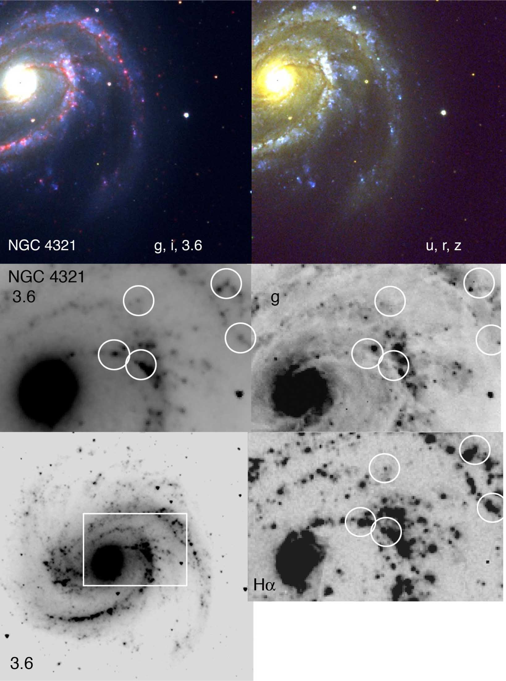
Figure 1: (Top left) color composite of NGC 4321 with SDSS $g$-band image for blue, SDSS $i$-band image for green, and IRAC $3.6\,\mu$m image for red, all with $0.75^{\prime\prime}$ pixels and combined by rotating, stretching, and aligning the optical images to match the infrared images. (Top right) SDSS color image remade from the u, r, and z SDSS filters using data from the SDSS webpage. (Middle left) sample region at $3.6\,\mu$m with circles highlighting $3.6\,\mu$m sources that do not appear in optical bands. (Middle right) The same circles on an SDSS $g$-band image (the circles are $\sim 10\times$ larger than the measurement rectangles). (Bottom left) $3.6\mu$m full image with a rectangle indicating the sample region. (Bottom right) Sample region again in H$\alpha$.

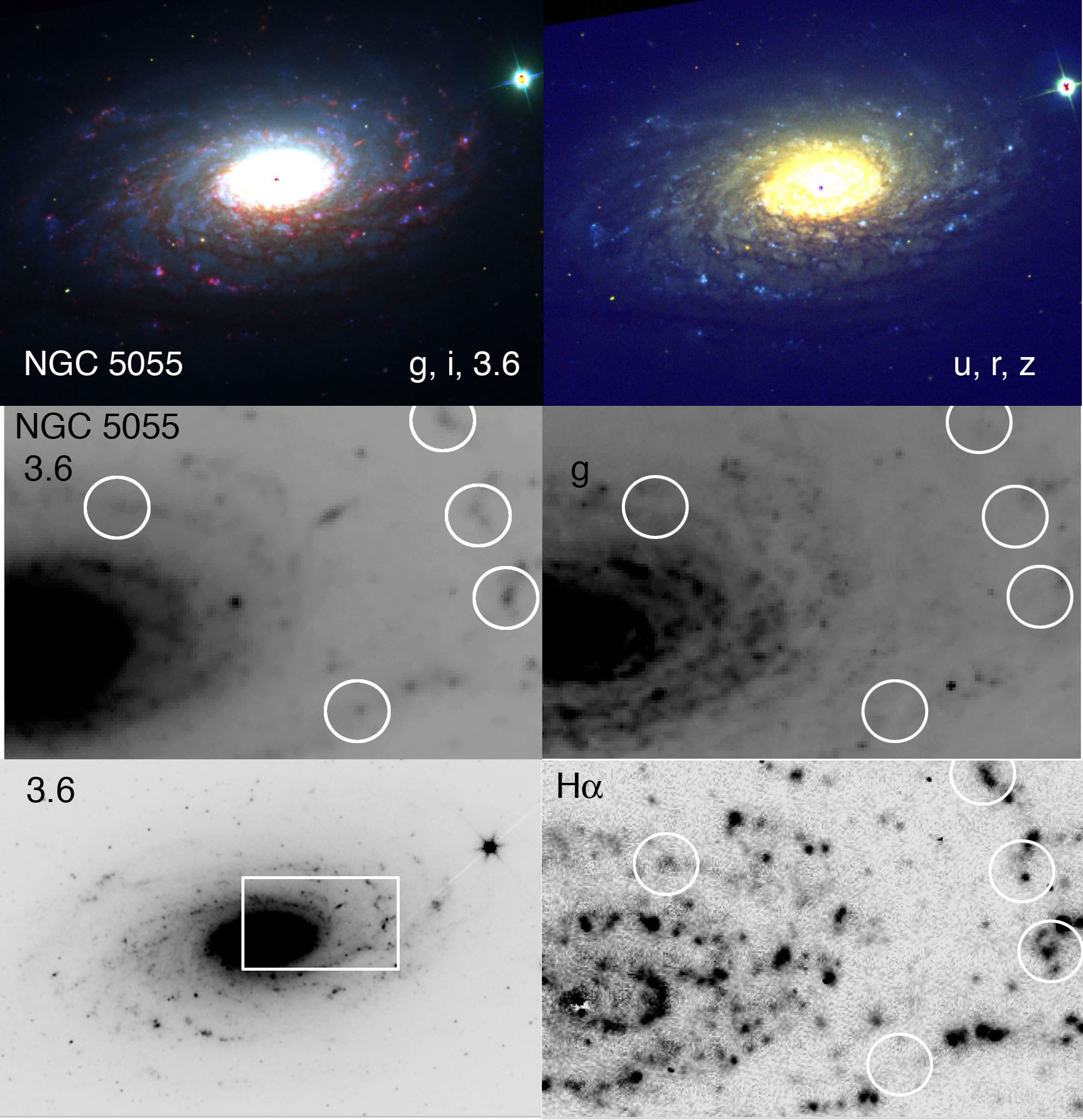
Figure 2: NGC 5055, as in Figure 1.

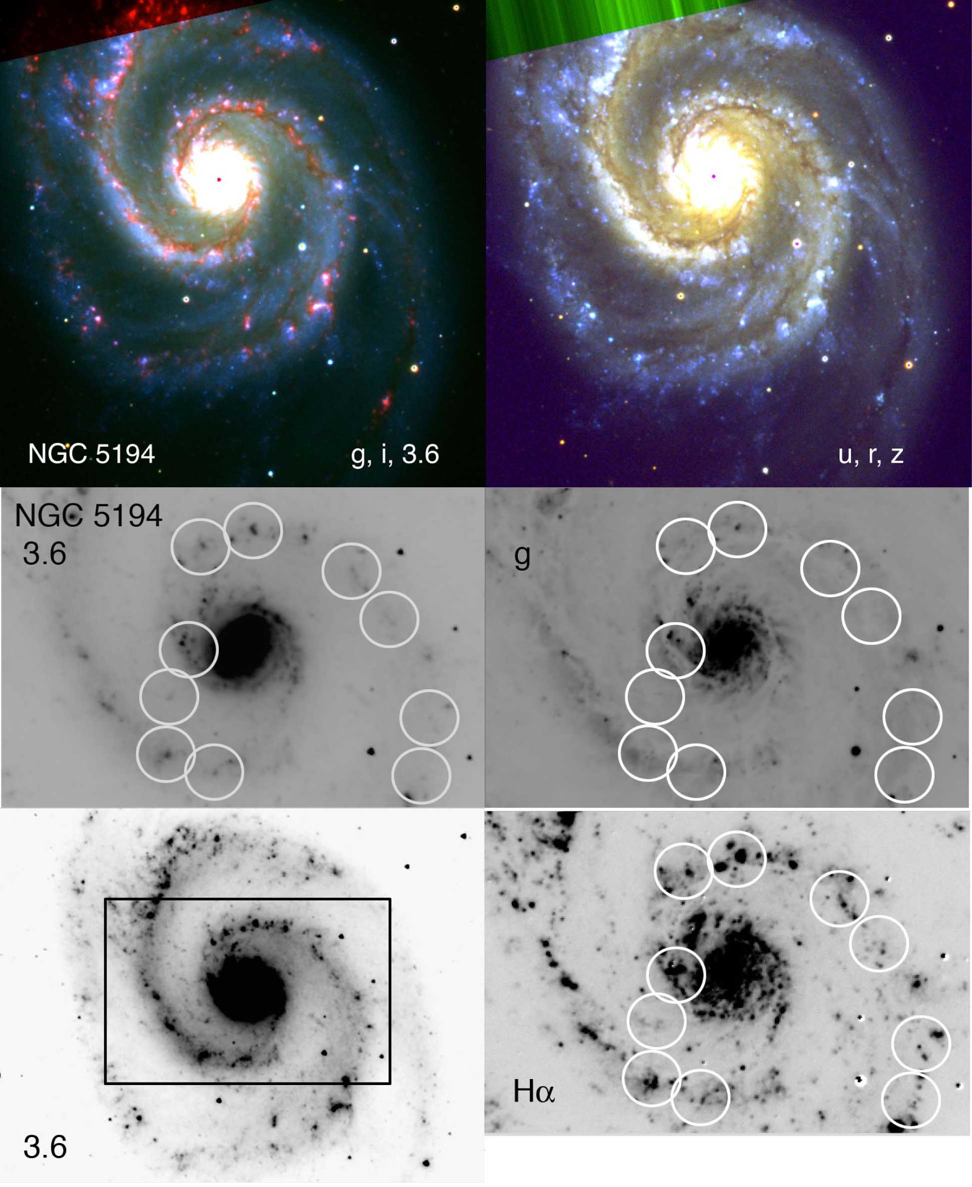
Figure 3: NGC 5194, as in Figure 1.

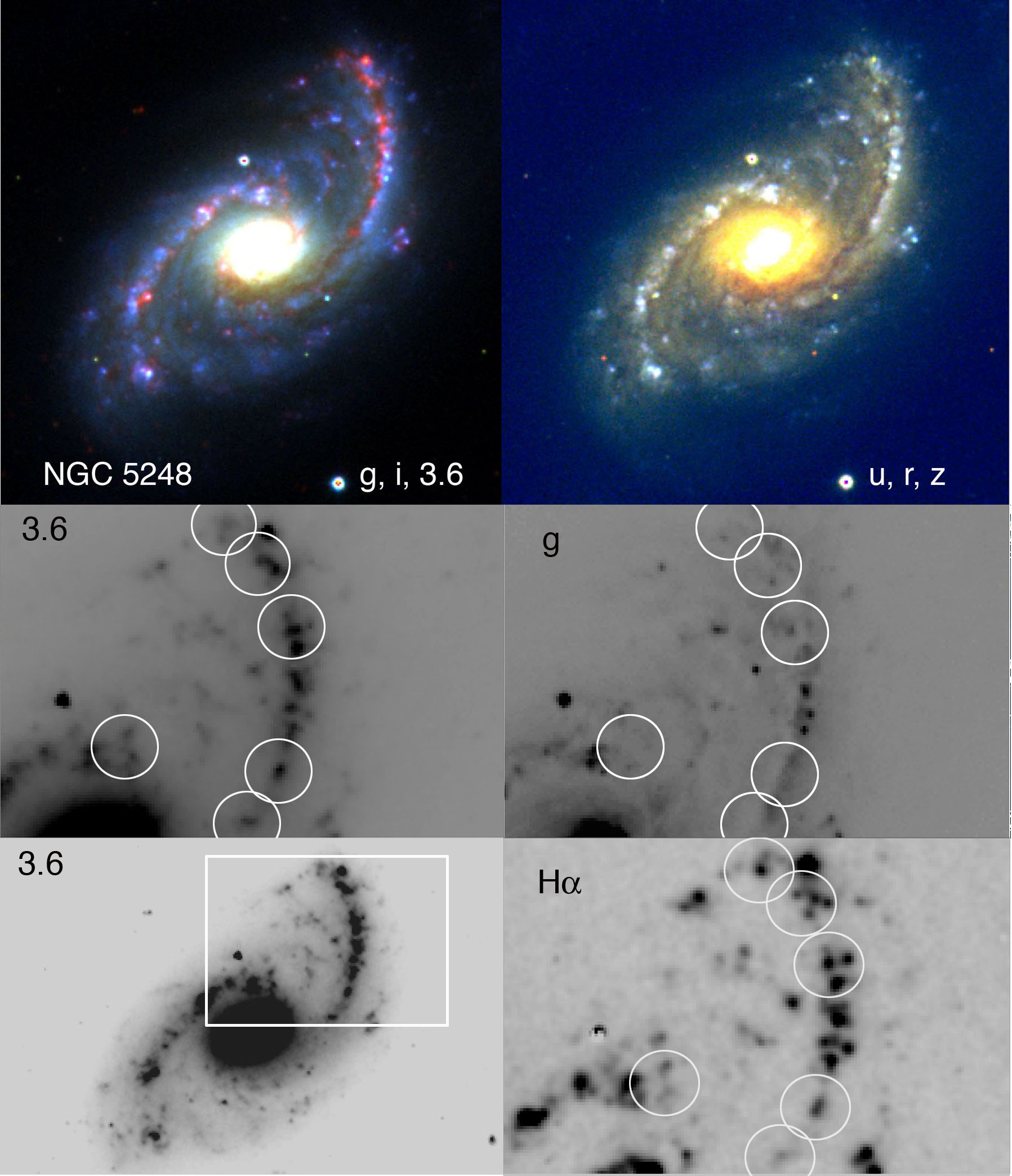
Figure 4: NGC 5248, as in Figure 1.

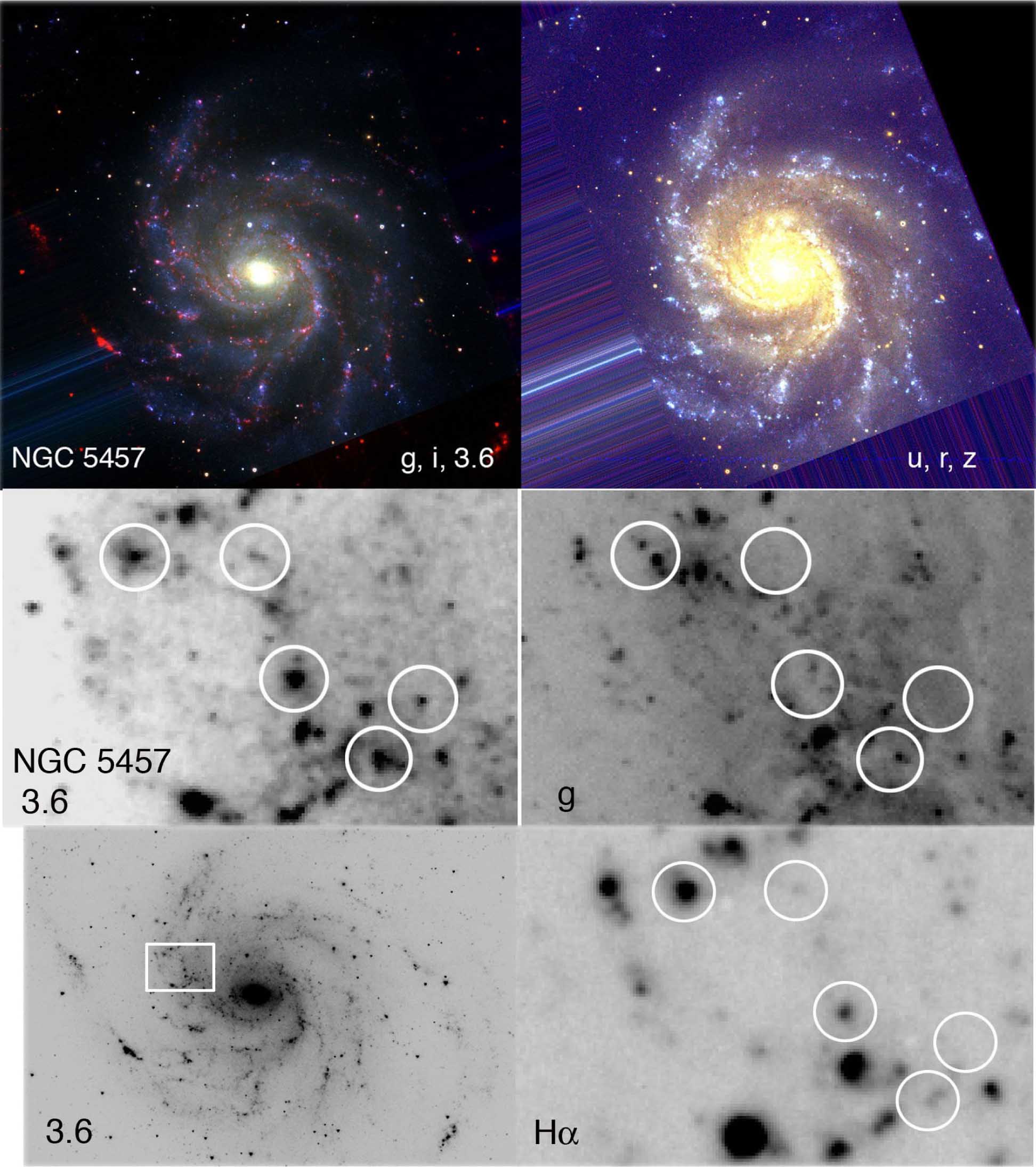
Figure 5: NGC 5457, as in Figure 1.

Figures 1–5 show the galaxies studied here. The color composites in the top left panels use SDSS $g$-band images for blue, SDSS $i$-band images for green, and IRAC $3.6\,\mu$m images for red. They all have $0.75^{\prime\prime}$ pixels and were combined into color images after first using IRAF wregister to rotate, stretch, and align the optical images to match the infrared images. The top right panel shows an image remade from the u, r, and z SDSS filters using data from the SDSS webpage (www.sdss.org). The middle left panel shows a sample region at $3.6\,\mu$m with circles highlighting $3.6\,\mu$m sources that do not appear in optical bands. These same circles are shown in the middle right panel on an SDSS $g$-band image. For clarity, these circles are $\sim 10\times$ larger than the measurement rectangles. The bottom left image is the $3.6\mu$m full image with a rectangle indicating the sample region, and the bottom right image is the sample region again in H$\alpha$.

Comparison of the middle panels in Figures 1–5 shows sources clearly visible at $3.6\mu$m but invisible at $g$-band. Sometimes part of a $3.6\mu$m source is visible at $g$ inside the circles, but the measuring rectangle was made on the part of the $3.6\mu$m source that was not visible at $g$ or at any other SDSS filter. Measurement rectangles are typically several arcseconds in length and width.

The identified sources appear to be embedded star-forming regions in the spiral arm dust lanes. They are visible at $3.6\,\mu$m because the extinction there is only $\sim 5$% of the $g$-band extinction (Cardelli et al., 1989). They are often visible in H$\alpha$ too, which is strange because that is an optical band, but H$\alpha$ emission can sometimes be more easily detected than optical starlight, and some of the H$\alpha$ could be from regions that are between and around the densest parts of the obscuring clouds. Higher resolution HST images show parts of these sources to be visible at optical bands, but the HST optical fluxes are still weak compared to the $3.6\mu$m fluxes because of a generally high obscuration.

The origin of the $3.6\mu$m emission is understood only in general terms. Some of it is from the Rayleigh-Jeans limit of the photospheric emission from young and old stars, some of it is from hot dust in young stellar disks and dense cores, and some is from PAH emission associated with the HII regions. We assume that the PAH part of the $3.6\mu$m emission is an independent measure of flux from the HII region. After subtracting the contribution from underlying stars (Mentuch et al., 2010), we can then determine the embedded cluster masses from the required ionizing fluxes. Comparison with the SDSS-band upper limits then gives a lower limit to the extinction.

The SDSS-band upper limit flux in a dust lane, $F_{\rm up}$, is taken to be the rms value of the SDSS pixel counts, $\sigma_{\rm px}$, multiplied by the counts-to-specific flux conversion factor, $C$, divided by the square root of the number of pixels, $N_{\rm px}^{0.5}$, and multiplied by the student-t value $t_{0.05}=1.7$ giving 95% probability that the mean count is less than $t_{0.05}\sigma_{\rm px}/N_{\rm px}^{0.5}$. That is, the probability that the mean flux from the source is less than the measured mean ($<F>\sim 0$ here) plus the increment $t_{0.05}\sigma_{\rm px}C/N_{\rm px}^{0.5}$ is 0.95. Here, $\sigma_{\rm px}$ comes from the IRAF measurement of the source counts. The value of $t_{0.05}$ is for a typical number of pixels in a source, $n\sim 20$, so the number of degrees of freedom for the student-t statistic is $n-1$, and the probability that the true mean $\mu$ is between $<F>-t_{0.05}\sigma_{\rm px}/N_{\rm px}^{0.5}$ and $<F>+t_{0.05}\sigma_{\rm px}/N_{\rm px}^{0.5}$ is 0.90. This is the same as saying that

$$F_{\rm up}=t_{0.05}\sigma_{\rm px}C/N_{\rm px}^{0.5}$$ (1)

with 95% confidence for $t_{0.05}=1.7$. The limiting magnitude is obtained from the limiting source flux using the usual AB conversion, mag$=-2.5\log_{10}F_{\rm up}-48.60$ for $F_{\rm up}$ in ergs cm^-2 s^-1 Hz^-1.

Table 2 lists the positions of the embedded sources, the number of pixels of $0.75^{\prime\prime}$ size in the measured rectangles, their fluxes, $S_{\nu}$, at $3.6\,\mu$m in $\mu$Jy, AB absolute magnitudes in IRAC $3.6\,\mu$m, AB absolute magnitude upper limits in the SDSS bands, and the H$\alpha$ luminosities measured from ground-based observations.

3 Method

Without optical detections of the embedded sources and only IRAC observations at $1.7^{\prime\prime}$ resolution from Spitzer and $1.25\mu$m observations at $2^{\prime\prime}$ resolution from 2MASS, we cannot uniquely determine the source ages, masses and extinctions. However, the sources are all embedded in spiral arm dust lanes and likely to be young (e.g., Scheepmaker, et al., 2009), as also implied by the H$\alpha$, so we searched over a range of ages, and for each age determined the cluster mass and extinction required to give the observed $3.6\mu$m and $1.25\mu$m fluxes using the conversion to intrinsic H$\alpha$ in Mentuch et al. (2010):

$$I_{\rm IR}(H\alpha)=\left(I[3.6\mu{\rm m}]-0.5I[1.25\mu{\rm m}]\right)/0.043$$ (2)

for $I$ in units of MJy/ster. That is, $I(3.6\mu{\rm m})$ and $I(1.25\mu{\rm m})$ in MJy/ster were measured from the background subtracted specific fluxes in each source (in units of $\mu$Jy from the image source counts), converted to MJy and divided by the area of the source in ster. The resulting $I_{\rm IR}(H\alpha)$ was then multiplied by a typical H$\alpha$ filter width in frequency units, $\Delta\nu$, which comes from the filter width in wavelength units, $\Delta\lambda=75$Å, converted to frequency with the equation $\Delta\nu=c\Delta\lambda/\lambda^{2}$. This gives the source H$\alpha$ flux in units of erg cm^-2 s^-1.

The intrinsic H$\alpha$ flux derived in this way from the IR, and the directly measured H$\alpha$ flux from ground-based observations, were converted to H$\alpha$ luminosities $L_{{\rm H}\alpha}$ by multiplying by $4\pi D^{2}$ for distance $D$, and then to observed ionization rates $S_{\rm obs}$ using the equation $S_{\rm obs}=7.3\times 10^{11}L_{{\rm H}\alpha}$ s^-1 (Kennicutt, 1998). These observed ionization rates were compared to stellar evolution models to determine intrinsic source properties.

For the stellar models, we used tables in Bruzual & Charlot (2003) for AB magnitude versus time in u,g,r,i, and z bands, which are given for a unit of solar mass in an initial cluster with a fully sampled Chabrier IMF and solar abundances. We also used the tables for Lyman continuum ionization rate versus time per unit initial solar mass, and residual stellar mass versus time per unit initial solar mass. The optical magnitudes were converted to luminosities per unit initial mass, and these along with the Lyman continuum rate and the residual stellar mass, were integrated over time up to the assumed age using a constant star formation rate. This integral over the model Lyman continuum rate per unit initial mass will be denoted by $S_{\rm m}(t)$, and the integral over the model residual mass per unit initial mass will be denoted by $M_{\rm m}(t)$.

The ratio of the observed ionization rate $S_{\rm obs}$ to the model rate $S_{\rm m}$ gives the correction factor to the model integrated mass, from which the required cluster mass can be derived:

$$M_{\rm cluster}=\left({{S_{\rm obs}}\over{S_{\rm m}(t)}}\right)M_{\rm m}(t)$$ (3)

The integrated luminosities in each SDSS band were found from the same ratio, e.g., $L_{\rm u}=(S_{\rm obs}/S_{\rm m}[t])L_{\rm m,u}(t)$ for u-band, and converted back to apparent magnitude. The resulting model magnitudes in all five SDSS bands were then subtracted from the observed magnitude limits in each band to get the minimum extinction in each band. These were all converted to g-band extinction using the extinction curve in Cardelli et al. (1989), and the results were averaged together. This extinction curve should be more appropriate for embedded sources than the gray type of extinction that comes from a partially transparent screen (Grosbøl & Dottori, 2012). The different limiting g-converted extinctions varied among the passbands by an average of 0.5 mag, presumably because the SDSS limits were not the same depth relative to the spectral energy distribution of the source.

4 Results

Table 3 gives the derived properties of the embedded sources listed in Table 2 for assumed ages of 3 Myr. The masses and average g-band-equivalent extinctions for the ground-based H$\alpha$ measurements are in columns 3 and 4, the masses and average g-band-equivalent extinctions for the $3.6\mu$m measurements are in columns 5 and 6, and the extinction needed in the HII region, measured at g-band, to produce the observed H$\alpha$ fluxes given the star forming regions measured at $3.6\mu$m, are in column 7. The sources with lower limits have upper limits for the directly observed H$\alpha$ fluxes (more on this below and in the footnote to table 3). All sources are observed at $3.6\mu$m.

The derived cluster masses increase with assumed age in the range from 1 to 10 Myr by about a factor of 2.5 for all sources (not shown). This is small enough for the likely age range that we consider here only masses for an assumed age of 3 Myr, as tabulated, with an uncertainty of a factor of 1.6 either way from unknown age effects. The mass differences obtained using the two methods, direct H$\alpha$ observations and H$\alpha$ inferred from $3.6\mu$m and $1.25\mu$m emissions, typically differed by a factor of 24 with the IR-based masses being larger. This difference amounts to an excess extinction of about 3.5 magnitudes for the direct H$\alpha$ compared to the IR-derived H$\alpha$.

Table 4 gives the embedded source masses and extinctions for the two types of measurements and the equivalent $g$-band extinction in the HII region to give H$\alpha$ consistent with $3.6\mu$m and $1.25\mu$m, averaged over all sources in each galaxy. The masses measured by direct H$\alpha$ observations average $2.4\times 10^{3}\;M_{\odot}$, and the masses measured by $3.6\mu$m and $1.25\mu$m observations and converted to H$\alpha$ average $5.0\times 10^{4}\;M_{\odot}$. The lower limits to the extinctions provided by the upper limits to the SDSS fluxes and the ground-based H$\alpha$ fluxes (column 3) are about zero, meaning that the H$\alpha$ measurements are consistent with the optical broad-band measurements in being highly extincted. In other words, given the stellar masses required to produce the (highly extincted) H$\alpha$ fluxes that were directly observed, the expected $u,g,r,i,z$ fluxes are comparable to the upper limits within a few tenths of a magnitude (the error bars in column 3 of Table 4). The lower limits to the extinctions derived from the $3.6\mu$m fluxes in comparison to the SDSS bands (column 5) are, on average, $\sim 3.8$ mag for all galaxies. This is comparable to the extinction in the HII region (column 6) because the HII emission is extincted by about the same amount as the SDSS bands.

We conclude that these dusty regions are obscuring young stellar associations with an average mass of $5.0\times 10^{4}\;M_{\odot}$ for an age of about 3 Myr. The average mass would be $4.2\times 10^{4}\;M_{\odot}$ for an age of 1 Myr and $1.3\times 10^{5}\;M_{\odot}$ for an age of 10 Myr. The average extinction to these regions in $g$-band is $\sim 3.8$ magnitudes.

5 Discussion

We consider possible star formation mechanisms as summarized in the introduction. Two of these mechanisms, the Parker and thermal instabilities, involve diffuse gas without self-gravity. While they may contribute to interstellar structure, they are not involved with rapid star formation because that requires self-gravity and collapsing cloud cores. The other mechanisms, gravitational instabilities and cloud impacts or collisions, involve strong self-gravity from an early stage, the first because whole dust lanes can be unstable to fragmentation along their lengths, and the second because collisions increase a cloud’s density and that can make the cloud gravitationally unstable.

The observation of bright embedded infrared sources in galactic spiral shocks implies that massive star formation begins quickly in the shocked gas – faster than the time delay usually inferred from the displacement between dust lanes or CO emission and visible HII regions (e.g., Egusa et al., 2009). The observed mass of $\sim 10^{4}-10^{5}\;M_{\odot}$ is comparable to the masses of more visible clusters and star-forming regions in normal galaxies.

In what follows, we consider two possible formation mechanisms for the observed star complexes. For both, the dust lanes are assumed to be shocks in spiral density waves. This is consistent with the streaming motions that are often observed in CO observations of these regions (e.g., Shetty et al., 2007). Most of the molecular clouds in the Milky Way spiral arms (Dame et al., 2001) seem related to spiral shocks too, considering their velocities and positions in the global spiral pattern (Bissantz et al., 2003). Their concentration in spiral arms is apparent in the face-on view of the Milky Way shown by Englmaier et al. (2011). Evidently, these local CO clouds would resemble dust lanes if they were viewed from outside the Milky Way.

The two mechanisms considered are (1) gravitational collapse of gas that accumulates behind the shock front in a spiral arm, and (2) compression and collapse of pre-existing clouds that hit these shock fronts. In the following discussion, we suggest that gravitational collapse of spiral arm shock fronts is too slow on kpc scales to account for the rapid onset of star formation that appears to be required for these embedded sources. The densest parts of the shocked gas could have collapsed into stars, however. Compression of interarm clouds that hit previously shocked gas could trigger the obscured sources faster. Additional considerations are needed to determine which mechanisms apply.

5.1 Gravitational Collapse of Spiral Arm Shock Fronts

Table 4 suggests that a typical value of optical extinction to an embedded dust lane source is $\sim 3.8$ mag. An embedded source with $A_{V}=3.8$ mag of extinction may be inside a dust cloud that has $\sim 8$ mag of extinction all the way through it if the source is centered. This makes the total column density through the cloud $\Sigma_{\rm gas}\sim 160\;M_{\odot}$ pc^-2 for $N(HI)=5.8\times 10^{21}E_{\rm B-V}$ (Bohlin et al., 1978), ratio of total-to-selective extinction $R_{\rm V}=3.1$ (Draine, 2003), and mean atomic weight 1.36. A typical dust lane width is $\sim 4$ pixels in Figures 1–5 (1 px$=0.75^{\prime\prime}$), which is $W\sim 150$ pc at a distance of 10 Mpc. The dust lane linear density is the product of these, $\mu=\Sigma_{\rm gas}W\sim 2.4\times 10^{4}\;M_{\odot}$ pc^-1, or $1.5\times 10^{19}$ g cm^-1. The critical line density for collapse of a filament is $\mu_{\rm c}=2\sigma^{2}/G$ for 1-dimensional velocity dispersion $\sigma$ (Inutsuka & Miyama, 1992, 1997). If $\sigma\sim 7$ km s^-1 in the shock, then $\mu_{c}$ is comparable to the observed line density. This suggests that spiral arm shock fronts are unstable to collapse along their lengths (Elmegreen, 1979; Kim et al., 2002; Kim & Ostriker, 2007; Renaud et al., 2013).

The result of this collapse would be one or more giant cloud complexes with masses equal to $\sim S\mu W$ for spacing $SW$ between the complexes along the arm (Inutsuka & Miyama, 1997). Taking $S\sim 4$ from the figures here and from Inutsuka & Miyama (1997), the resulting cloud mass is $\sim 1.4\times 10^{7}\;M_{\odot}$. If we consider a typical efficiency of 2% for the star-forming complex, then a stellar mass of $\sim 3\times 10^{5}\;M_{\odot}$ results, large enough to account for what we observe.

The key to star formation in spiral arm dust lanes is that it has to happen quickly, before the spiral arm passes and the shocked gas decompresses in the interarm. This is a strong constraint if the spiral wave is steady. Not all compressed regions will be part of a steady flow, however. If a dust lane is sufficiently self-gravitating, then it can remain intact as a giant cloud complex even when it enters the interarm region, making its lifetime longer than the arm crossing time. Such shocks would not be steady but would cycle between gas build up, collapse, and dispersal. If the lifetime of the compressed state is long enough, then interarm protrusions and spurs result (Wada & Koda, 2004; La Vigne et al., 2006; Shetty & Ostriker, 2006; Dobbs & Bonnell, 2006; Lee & Shu, 2012; Renaud et al., 2013) with star formation lingering in the interarm regions.

Egusa et al. (2011) observed M51 with 30 pc resolution and could see cloud build-up from small interarm CO clouds to giant molecular associations as the gas flowed into and through the spiral arms. With 780 pc resolution, the excitation state of M51 CO clouds changes from low in the interarm regions to high in the arms, corresponding to an increase in density and/or temperature with increasing star formation activity (Koda et al., 2012). There is also an indication in M51 of dense CO gas just before prominent spiral arm star formation; the map in Figure 6 of Koda et al. (2012) shows regions with highly excited CO and low $24\,\mu$m emission. These regions appear to be centered on dust lanes, although their exact spatial distribution is uncertain because the 780 pc resolution scale of the map is much larger than a dust lane. These regions avoid the parts of the dust lanes where we identify the brightest embedded sources, but that is expected from the lack of $24\,\mu$m emission in the Egusa et al. (2011) sources. Similarly, Hirota et al. (2011) observed molecular clouds in IC 342 turn from weakly self-gravitating in the interarm regions to strongly self-gravitating and star-forming in the arms.

We now consider when the collapse of density wave-shocked gas is fast enough to make stars in the steady state case. This requires a comparison between the collapse time of this gas and its dwelling time in the arm.

The dwelling time for gas in a dust lane is the arm-to-arm time multiplied by the ratio of the gas mass inside the dust lane within some radial interval to the total gas mass from one arm to the next in that radial interval. This relationship is from the continuity equation. Because of streaming motion along the arm in the dust lane, this dwelling time is longer than the purely geometric time obtained from the ratio of the angular thickness of the dust lane measured from the galaxy center divided by the angular rate of the spiral pattern relative to the gas.

The ratio of the dust lane mass to the total arm-to-arm gas mass in a radial interval equals the ratio of the dust lane column density to the average column density, multiplied by the relative angular extent of the dust lane. In the star-forming part of the main disk of most spiral galaxies, the V-band extinction averaged in azimuth is typically about 1 magnitude. Recall that the column density for general extinction $A_{\rm V}$ equals $20A_{\rm V}\;M_{\odot}$ pc^-2 in units of surface density, and an average value of $20\;M_{\odot}$ pc^-2 for spiral galaxy disks is typical inside the molecular zone (Bigiel et al., 2008). For a general case like this, the ratio of column densities is then approximately $A_{\rm V,dl}/(1\;{\rm mag})$ for $A_{\rm V,dl}$ in the dust lane. The arm-to-arm distance is $\pi R$ for a two-arm spiral at radius $R$. Taking $R=4$ kpc as representative, the relative dust lane thickness is $W/\pi R\sim 1$% with $W=150$ pc from above. Thus the fraction of the gas mass in the dust lane, which is also the fraction of the arm-to-arm time in the dust lane, is approximately $0.01A_{\rm V,dl}$. The arm-to-arm time is $\sim 120$ Myr for a position at $R\sim 4$ kpc that is halfway to corotation where the galaxy rotation speed is $\sim 200$ km s^-1. Then the dwelling time for gas in the dust lane is $\sim 1.2A_{V,dl}$ Myr. In general, the dust lane flow-through time is $(W/V_{\rm rel})\times(A_{\rm V,dl}/A_{\rm V,ave})$ for dust lane width $W$, azimuthal speed $V_{\rm rel}$ of the spiral arm relative to the gas, and average extinction through the disk at the radius of the dust lane, $A_{\rm V,ave}$. This result does not depend on $R$ explicitly. If $W$ is in pc and $V_{\rm rel}$ is in km s^-1, then the unit of this flow-through time is approximately in Myr.

The fraction of the time that gas spends in the vicinity of a spiral arm can be fairly high for a strong arm. For example, a CO map of the galaxy shown in Figure 4, NGC 5248 (Kuno et al., 2007), has two spiral arms midway out with $\sim 12$ K km s^-1 integrated intensities that occupy about 20%-25% of the azimuthal distance to the next arm, and it shows interarm regions with less than 3 K km s^-1. Thus the arms contain about half of the gas at that radius ($(12/3)*0.25=0.5$), and the arm dwelling time is half of the arm-to-arm time if most of the gas is molecular. This fraction would be lower if the $X$-factor that converts CO to H₂ is lower in the arms than in the interarms because of greater CO temperatures in the arms. Using $V_{\rm rel}\sim 100$ km s^-1, which is half of the rotation speed of NGC 5248 (Nishiyama et al., 2001), assuming this position is half the distance to co-rotation, and assuming a galactocentric distance of 1 arcmin $\sim 4$ kpc, the arm-to-arm time is 126 Myr and the arm dwelling time could be about 60-70 Myr. In the spiral arms of M51 (Koda et al., 2011), the dust lanes appear as thin ribbons of CO emission nearly resolved by CARMA. They occupy about 10% of the azimuthal angle and have 5 to 10 times the average interarm intensity in CO. Thus even the thin CO arms in M51 contain 30% to 50% of the molecular mass at that radius, and because most of the gas in this galaxy is molecular (Koda et al., 2009), this is also approximately the fraction of the arm-to-arm time spent in the dust lanes (unless the $X$-factor varies).

The dwelling time in a spiral arm has to be compared with the timescale for self-gravitational collapse. The latter is about $S(G\rho)^{-1/2}$ for length-to-width ratio $S$ along the dust lane and for density $\rho$. The factor $S$ comes from the average equivalent density $\rho_{\rm sph}$ in a sphere containing the fragment, considering that the collapse time is $\sim(G\rho_{\rm sph})^{1/2}$ for that average. In agreement with this, Inutsuka & Miyama (1997) show one case of a filament with a collapse to a singularity in $12.3/(4\pi G\rho)^{1/2}$, which is $3.5/(G\rho)^{1/2}$, giving $S\sim 3.5$ in their case (see also Pon et al., 2012). The average dust lane density is the extinction through the disk, $A_{\rm V,dl}$, converted into grams cm^-2, divided by the line-of-sight thickness, which is $H\sim 70$ pc for a typical molecular disk. For $H$ in parsecs, this density is $1.4\times 10^{-21}A_{\rm V,dl}/H$ g cm^-3, and the collapse time is $3.3S(H/A_{\rm V,dl})^{1/2}$ Myr, or some $\sim 10S$ Myr if $H\sim 70$ pc and $A_{\rm V,dl}\sim 8$ mag (i.e., using $A_{\rm V,dl}\sim 2<A_{\rm g}>$ or $2\Delta A_{\rm g}$ from table 4).

For gravitational collapse in a dust lane, the collapse time has to be less than the flow-through time, which means $A_{\rm V,dl}^{1.5}>3.3SH^{1/2}A_{\rm V,ave}V_{\rm rel}/W$ or $A_{\rm V,dl}>18$ mag for $S=4$, $H=70$ pc, $A_{\rm V,ave}=1$ mag, $V_{\rm rel}=100$ km s^-1, and $W=150$ pc. This result implies that sufficiently dense spiral shocks, i.e., those with extinctions through the disk greater than $\sim 18$ mag for these numbers, should have time to collapse along their lengths into new cloud complexes. Because self-gravity is important from the start in such an instability, the cloud complexes that form will also be strongly self-gravitating, and should form stars at an accelerating pace while they collapse further.

Recall that our sources imply $A_{\rm A,dl}\sim 8$ mag on average, considering we see the foreground extinction equal to half of this value. This extinction is slightly less than the critical value of 18 mag derived above, suggesting that the dust lanes we observe are only marginally unstable to collapse in the short time they have. If the line-of-sight cloud thicknesses were much smaller than the assumed $H\sim 70$ pc, such as the size of a giant molecular cloud, $\sim 10$ pc, then $A_{\rm V,dl}\sim 9$ pc, and this would be closer to our observations. In either case, the observed dust lanes do not appear to be strongly self-gravitating and in the process of rapid collapse. They could be forming stars only in the initially dense regions that were most unstable before they entered the spiral arm. Such partial collapse is consistent with the spiral shock models by Bonnell et al. (2013) and with the growing evidence for star formation in marginally bound or unbound molecular clouds (i.e., but which are still unstable to collapse in their cores; Dobbs et al., 2011).

Kim & Ostriker (2002) ran simulations showing the steady accumulation of shocked gas in spiral arms, with dust lane density perturbations building up over several rotation periods from initially small amplitudes. Eventually the irregularities caused by gaseous self-gravity led to the formation of giant, self-gravitating clouds. This is essentially the process we have in mind here for the formation of the observed embedded sources.

Elmegreen (2012) showed examples of beads-on-a-string of star formation along spiral arms of all types, ranging from two-arm grand design spirals to multiple, long-arm spirals, to flocculent spirals (see also Elmegreen & Elmegreen 1983). Beads-on-a-string patterns were studied in detail by Elmegreen et al. (2006) using IRAC images like those considered here. In many images from the Galaxy Evolution Explorer satellite (GALEX; Martin et al. 2005), one gets the impression that most star formation is in complexes that are strung out along spiral arms in a semi-regular fashion. Interstellar magnetic fields may be involved in this regularity (Efremov, 2010). Evidently, there is a close resemblance between spiral arm star formation on kpc scales and filamentary star formation (André et al, 2010) inside molecular clouds on parsec scales.

5.2 Pressurized Gravitational Collapse of Incident Massive Cloud Complexes

Compression and collapse of an incident interarm cloud can be faster than the collapse time calculated above for an initially uniform dust lane. The compression time $t_{\rm comp}$ is the cloud size $R_{\rm cloud}$ divided by the relative perpendicular speed between the cloud and the spiral arm, $V_{\rm perp}$. For a relative azimuthal speed between the cloud and the arm, $V_{\rm rel}=100$ km s^-1 as above, the perpendicular speed is $V_{\rm rel}\sin i\sim 30$ km s^-1 when the spiral arm pitch angle is $i=20^{\circ}$. Then $t_{\rm comp}\sim 3$ Myr for $R_{\rm cloud}\sim 100$ pc. Collapse would follow compression quickly because the compressed cloud density is high, approximately equal to the product of the interarm cloud density, $20A_{\rm V,ia}/H$ (in $M_{\odot}/$pc³ for an interarm cloud extinction $A_{\rm V,ia}$ and line-of-sight thickness $H$ in pc) multiplied by the square of the ratio of the perpendicular compression speed to the cloud thermal speed, $\left(V_{\rm perp}/v_{\rm th}\right)^{2}$. For $A_{\rm V,ia}\sim 1$ mag, $H=70$ pc, $V_{\rm perp}=30$ km s^-1, and $v_{\rm th}=3$ km s^-1, the compressed cloud density is $n_{\rm comp}\sim 850$ atoms cm^-3 and the cloud collapse time, measured as $(G\rho_{\rm comp})^{-1/2}$, is $\sim 2.8$ Myr. If such a density extends for $H=70$ pc along the line of sight, then the extinction through the disk would be $A_{\rm V}\sim 100$ mag and the extinction to an embedded source $\sim 50$ mag. This is significantly larger than what we observe here for the clouds on $W\sim 150$ pc scales, but could apply in their cores.

The original picture of cloud compression in spiral shocks was based on simulations by Woodward (1976) of a small diffuse cloud engulfed by a rapidly moving, infinitely-extended shock front. The cloud is compressed by the post-shock gas and forms a cometary structure, with the head collapsing into stars. Many simulations have confirmed this basic process. Spiral arms do not typically show cometary clouds and the dust lanes surrounding the embedded sources discussed here are not cometary. Still, the basic model of cloud compression upon impact with an existing spiral arm dust lane (from a previous shock) seems generally valid.

The interarm clouds in Figures 1–5 are spiral-like with large cloud complexes distributed along their lengths. This interarm structure is also evident from well-resolved maps of IR (Block et al., 1997) and CO (Koda et al., 2011), as in the case of M51. Such shapes are remnants of dust lane structures, secondary shocks, and spurs from the previous arms (La Vigne et al., 2006; Shetty & Ostriker, 2006; Dobbs & Bonnell, 2006). Interarm cloud complexes can be moderately massive: $M_{\rm cloud}=6\times 10^{5}\;M_{\odot}$ if $R_{\rm cloud}\sim 100$ pc and $A_{\rm V,ia}=1$ mag. The most opaque interarm clouds may contain $\sim 10^{7}\;M_{\odot}$ and have a substantial molecular fraction (e.g., Koda et al., 2011).

The observed masses of the largest embedded complexes found here are consistent with interarm cloud compression. The pre-collision clouds would have to be $\sim 50$ times more massive than the observed stellar masses, considering a star formation efficiency on $\sim 100$ pc scales of 2%. To form a $\sim 10^{5}\;M_{\odot}$ star complex inside a dust lane (Table 4), the previous interarm cloud would have to contain $5\times 10^{6}\;M_{\odot}$. Such a cloud, if spherical, would be $\sim 280$ pc in diameter if its average extinction is $A_{\rm V,ia}=1$ mag. With such a size in two dimensions, the cloud would form a $\sim 280$ pc long dust filament when it hits the spiral arm, and then the collapse to star formation would be like the dust lane collapse discussed above, with motions along its length and a factor $S\sim 4$ geometric dilution of the collapse time.

5.3 Regular spacing of star formation along spiral arms

Regular spacing of large star complexes along spiral arms, as occasionally seen in Figures 1–5 and in other galaxies, implies that an instability might be involved and we are seeing the fastest growing wavelength of that instability (e.g., Wada & Koda, 2004; Shetty & Ostriker, 2006; Lee & Shu, 2012; Renaud et al., 2013). The presence of several young sources in this string implies that the instability operates all along the length of the pattern with a nearly uniform starting time, to within some variation equal to the instability time or the arm dwelling time. Such simultaneity requires that the dust lanes with regular star formation evolved within this time interval, that is, they built up, fragmented, and turned into stars along the length of the regular pattern within several tens of Myrs. After this, another dust lane would be expected to build up to replace it using fresh interarm gas. This would be the case for a continuously moving spiral arm that accumulates gas, dumps it into star complexes and then accumulates more gas. Alternatively, the whole stellar and gaseous arm could have formed recently as a result of a spiral instability in the disk (Baba et al., 2013). Then the arm structure itself would be fairly young (although the stellar populations in it would be mostly old) and it could just now be forming its first string of star formation, i.e., within the last $\sim 30$ Myr. In both cases, the instability would be slow compared to the dynamics of star formation, so the OB associations that form would be in various stages of obscuration and break-out, ranging from embedded for the youngest to fully exposed with adjacent cloud debris for the oldest in the same arm segment.

In cases without a regular spacing along spiral arms, a similar time sequence may occur with spiral-shocked gas followed by partial cloud collapse, star formation, and cloud dispersal, but with more of a distributed starting time. Then there will be different phases in this process at different positions along the arm. There could also be other processes acting, such as direct compression of interarm clouds, which would be randomly placed with respect to the regular structures.

6 Conclusions

A search for emission at $3.6\mu$m that has no associated optical counterpart in SDSS images and only weak emission at H$\alpha$ revealed 73 sources that are likely to be young star formation regions embedded in molecular clouds. The clouds appear as dark dust lanes in the spiral arms. The intrinsic H$\alpha$ emission of each source was estimated from the $3.6\mu$m and $1.25\mu$m emissions using the method of Mentuch et al. (2010), and the luminosity of the associated stars was determined after assuming an age in the range of 1 to 10 Myr. This stellar luminosity, combined with upper limits from the SDSS images, gave lower limits to the extinction and stellar mass. The observed H$\alpha$, compared with the H$\alpha$ estimated from $3.6\mu$m and $1.25\mu$m, gave a consistent value for the extinction, which is apparently near the estimated lower limit (or else the H$\alpha$ would not be observed either).

The average mass of an embedded source was found to be $5\times 10^{4}\;M_{\odot}$ and the average extinction at $g$-band is $3.8$ mag. These sources are often parts of regular strings of star formation with additional embedded sources and other sources in various stages of lower obscuration. Two mechanisms for triggering this star formation were considered: gravitational collapse of spiral density wave-shocked gas and gravitational collapse of compressed incident clouds. The spiral shock model suggests that the clouds we are observing are not strongly self-gravitating because they have not had enough time after their formation in the spiral arm. Still, collapse should occur in dense cores of these clouds even if the overall cloud complexes are weakly bound. This is consistent with recent ideas that star formation occurs in the dense cores of generally unbound molecular clouds. The incident cloud model is also consistent with our observations if, again, the shock compression and collapse to star formation occurs primarily in unseen dense cores.

The regular distribution of star formation along spiral arms, including the embedded sources as well as the exposed sources, suggest that a mild instability is operating to form weakly bound molecular clouds simultaneously along kpc lengths. Simultaneity on these scales requires a uniform initial starting time for the instability, to within the unstable growth time or the flow-through time. In that case the arm could be relatively young, or the shock front in the arm could be relatively new.

B.G.E. is grateful to E. Mentuch for clarifications about the analysis method that her team proposed. E.A. and A.B. thank the CNES for financial support. We acknowledge financial support to the DAGAL network from the People Programme (Marie Curie Actions) of the European Union’s Seventh Framework Programme FP7/2007-2013/ under REA grant agreement number PITN-GA-2011-289313. This research made use of the NASA/IPAC Infrared Science Archive, which is operated by the Jet Propulsion Laboratory, California Institute of Technology, under contract with the National Aeronautics and Space Administration. This work is based in part on observations made with the Spitzer Space Telescope, which is operated by the Jet Propulsion Laboratory, California Institute of Technology under a contract with NASA. This research made use of the NASA/IPAC Extragalactic Database which is operated by JPL, Caltech, under contract with NASA. This research made use of data products from the Two Micron All Sky Survey, which is a joint project of the University of Massachusetts and the Infrared Processing and Analysis Center/California Institute of Technology, funded by the National Aeronautics and Space Administration and the National Science Foundation. Funding for the SDSS and SDSS-II has been provided by the Alfred P. Sloan Foundation, the Participating Institutions, the National Science Foundation, the U.S. Department of Energy, the National Aeronautics and Space Administration, the Japanese Monbukagakusho, the Max Planck Society, and the Higher Education Funding Council for England. The SDSS Web Site is http://www.sdss.org/. The SDSS is managed by the Astrophysical Research Consortium for the Participating Institutions. The Participating Institutions are the American Museum of Natural History, Astrophysical Institute Potsdam, University of Basel, University of Cambridge, Case Western Reserve University, University of Chicago, Drexel University, Fermilab, the Institute for Advanced Study, the Japan Participation Group, Johns Hopkins University, the Joint Institute for Nuclear Astrophysics, the Kavli Institute for Particle Astrophysics and Cosmology, the Korean Scientist Group, the Chinese Academy of Sciences (LAMOST), Los Alamos National Laboratory, the Max-Planck-Institute for Astronomy (MPIA), the Max-Planck-Institute for Astrophysics (MPA), New Mexico State University, Ohio State University, University of Pittsburgh, University of Portsmouth, Princeton University, the United States Naval Observatory, and the University of Washington.

Table 1: Galaxies Observed for Embedded Sources

Galaxy	Type	Radius (arcsec)	Inc. (deg)	D (Mpc)	pixel (pc)	$B_{\rm T,0}$ (mag)	$M_{\rm B}$ (mag)	$M_{3.6\,u{\rm m}}$ (mag)
NGC 4321	SXS4	222	32	20.9	76	9.98	-21.62	-22.57
NGC 5055	SAT4	377	55	7.54	27	9.03	-20.36	-21.37
NGC 5194	SAS4P	336	52	7.54	27	8.67	-20.72	-21.83
NGC 5248	SXT4	184	44	15.4	56	10.63	-20.31	-21.23
NGC 5457	SXT6	865	21	4.94	18	8.21	-20.26	-20.65

Table 2: Measurements of Embedded Sources

Galaxy
Region	RA	Dec	$N_{\rm px}$	$S_{\nu}(3.6\,\mu{\rm m})$	$M_{\rm 3.6}$	$u$	$g$	$r$	$i$	$z$	$\log_{10}L_{H\alpha}$
				($\mu$Jy)							(erg s-1)
NGC 4321
1	12:22:50.498	15:50:24.03	30	282	-13.83	-6.09	-6.44	-6.60	-6.80	-7.05	38.47
2	12:22:50.238	15:50:19.91	36	240	-13.65	-6.37	-6.74	-7.13	-7.02	-7.36	38.66
3	12:22:48.705	15:50:14.28	16	220	-13.56	-5.88	-6.04	-6.54	-6.74	-7.20	38.19
4	12:22:48.471	15:50:11.66	24	254	-13.71	-6.23	-6.77	-7.21	-7.30	-7.80	$<37.73$
5	12:22:48.263	15:50:09.03	25	297	-13.88	-6.75	-7.20	-7.35	-7.31	-7.80	38.09
6	12:22:48.238	15:49:47.28	20	219	-13.55	-5.93	-5.84	-6.80	-6.49	-6.97	38.14
7	12:22:47.614	15:49:48.78	16	166	-13.25	-6.35	-6.24	-7.13	-6.79	-7.44	38.34
8	12:22:46.575	15:48:55.15	9	32	-11.48	-5.58	-5.91	-5.85	-5.93	-7.25	$<36.75$
9	12:22:46.445	15:48:50.65	6	32	-11.45	-6.98	-5.23	-5.62	-6.63	-7.74	$<36.94$
10	12:22:48.654	15:48:04.53	16	102	-12.72	-5.63	-6.26	-7.10	-7.43	-7.39	$<37.43$
11	12:22:56.241	15:48:10.16	48	1445	-15.60	-6.20	-6.30	-7.20	-6.82	-7.10	38.74
12	12:22:51.642	15:49:33.41	20	596	-14.64	-6.98	-7.13	-7.54	-7.27	-7.56	38.57
13	12:22:52.603	15:49:39.04	30	364	-14.10	-5.72	-6.14	-6.68	-6.79	-7.14	38.38
14	12:22:51.797	15:50:05.66	9	60	-12.14	-6.50	-6.41	-7.01	-7.08	-7.93	37.73
15	12:22:54.656	15:49:33.04	9	383	-14.16	-6.37	-7.41	-8.07	-8.54	-9.13	38.40
NGC 5055
1	13:15:50.565	42:01:16.91	6	63	-9.98	-7.05	-6.38	-7.38	-7.94	-9.15	$<37.11$
2	13:15:49.657	42:01:12.78	12	187	-11.17	-7.95	-8.40	-9.09	-9.31	-9.99	37.26
3	13:15:48.512	42:01:10.91	36	651	-12.52	-5.52	-5.39	-5.95	-6.69	-7.74	37.89
4	13:15:42.286	42:01:31.89	9	211	-11.30	-6.69	-6.36	-7.51	-7.38	-7.77	36.78
5	13:15:38.651	42:01:42.75	12	306	-11.70	-7.93	-7.58	-8.36	-8.34	-9.21	37.82
6	13:15:39.155	42:01:58.50	30	1239	-13.22	-6.58	-7.25	-7.59	-7.57	-8.06	38.13
7	13:15:38.886	42:02:05.63	12	507	-12.25	-5.42	-5.42	-6.68	-6.09	-7.34	38.40
8	13:15:39.861	42:02:19.51	6	129	-10.77	-6.52	-5.98	-6.56	-7.27	-8.40	37.77
9	13:15:39.895	42:02:19.13	9	201	-11.25	-7.98	-8.24	-8.72	-8.74	-9.07	37.58
10	13:15:40.534	42:02:40.14	20	555	-12.35	-7.11	-7.11	-7.61	-7.81	-8.56	38.23
11	13:15:47.401	42:02:19.91	16	175	-11.09	-5.47	-5.45	-6.74	-6.51	-7.45	37.99
12	13:15:50.364	42:02:25.53	6	118	-10.67	-7.16	-7.68	-8.14	-8.60	-9.43	37.59
13	13:15:53.326	42:02:22.53	12	157	-10.98	-8.44	-8.35	-9.36	-8.49	-9.29	$<36.47$
14	13:15:43.330	42:00:57.40	25	852	-12.82	-6.65	-7.08	-7.22	-7.34	-8.49	38.73
15	13:15:56.958	42:00:52.14	16	350	-11.85	-6.54	-6.98	-8.27	-8.20	-8.93	37.42
16	13:15:52.281	42:01:19.53	12	346	-11.84	-6.97	-7.55	-7.86	-7.87	-7.87	38.10
NGC 5194
1	13:29:54.725	47:12:36.45	16	994	-12.98	-7.76	-8.25	-8.86	-8.67	-9.03	38.50
2	13:29:52.038	47:12:42.82	20	1502	-13.43	-9.31	-9.33	-9.95	-9.46	-9.59	38.51
3	13:29:46.997	47:12:23.32	12	278	-11.60	-6.39	-7.25	-7.63	-7.74	-8.84	38.03
4	13:29:45.231	47:11:58.94	9	118	-10.67	-6.41	-6.89	-7.69	-7.76	-8.36	37.66
5	13:29:44.864	47:11:55.18	16	221	-11.35	-6.49	-6.98	-7.53	-7.80	-8.45	37.94
6	13:29:45.489	47:11:55.56	12	57	-9.88	-5.88	-7.11	-7.64	-7.68	-8.27	37.51
7	13:29:42.953	47:11:05.30	9	84	-10.30	-6.48	-7.20	-7.21	-7.04	-7.84	37.82
8	13:29:43.359	47:10:33.80	9	132	-10.79	-6.48	-6.66	-7.02	-7.21	-8.32	37.80
9	13:29:54.098	47:10:36.07	20	662	-12.54	-7.14	-7.89	-8.50	-8.49	-8.88	37.99
10	13:29:56.526	47:10:45.82	42	2465	-13.97	-8.45	-9.23	-9.62	-9.67	-9.81	38.58
11	13:29:56.453	47:11:15.82	30	322	-11.76	-7.26	-7.15	-7.79	-7.70	-8.64	38.09
12	13:29:55.828	47:11:44.70	12	1202	-13.19	-8.02	-8.47	-9.62	-9.60	-9.42	38.56
NGC 5248
1	13:37:29.691	8:54:30.29	28	466	-13.71	-9.08	-9.15	-9.71	-9.57	-10.22	38.44
2	13:37:29.033	8:54:20.91	24	766	-14.25	-8.95	-9.59	-10.10	-10.25	-10.46	38.53
3	13:37:28.780	8:53:27.66	42	1120	-14.66	-10.00	-10.68	-10.86	-10.79	-10.98	38.93
4	13:37:29.286	8:53:14.91	15	278	-13.15	-8.29	-8.21	-8.60	-8.94	-9.86	38.60
5	13:37:30.374	8:52:50.16	20	140	-12.40	-8.65	-8.78	-9.33	-8.91	-9.65	38.37
6	13:37:32.601	8:52:43.41	20	157	-12.53	-8.85	-8.81	-9.35	-9.51	-10.39	38.23
7	13:37:32.930	8:52:32.54	24	291	-13.20	-9.41	-9.65	-10.42	-10.10	-10.46	39.02
8	13:37:34.929	8:53:00.29	15	263	-13.09	-8.94	-9.19	-9.55	-9.51	-9.94	38.65
9	13:37:34.575	8:53:06.29	16	208	-12.83	-8.54	-8.90	-8.64	-9.02	-9.70	38.46
10	13:37:35.106	8:52:20.54	12	157	-12.53	-8.55	-7.88	-8.69	-8.71	-9.34	38.50
11	13:37:33.967	8:53:12.29	6	40	-11.04	-7.56	-7.71	-7.95	-8.58	-9.27	37.61
12	13:37:31.386	8:53:37.04	42	315	-13.29	-9.24	-9.26	-9.55	-9.45	-11.57	38.75
13	13:37:31.285	8:53:31.41	30	155	-12.52	-9.15	-9.28	-9.72	-9.77	-10.32	38.55
NGC 5457
1	14:03:07.750	54:22:43.86	20	227	-10.46	-5.71	-5.56	-6.35	-7.35	-7.76	37.62
2	14:03:05.818	54:22:45.35	12	108	-9.65	-5.75	-5.14	-5.28	-5.93	-6.90	$<37.03$
3	14:03:04.745	54:22:45.73	16	150	-10.01	-5.73	-5.22	-5.93	-6.09	-7.50	$<37.66$
4	14:03:03.843	54:22:47.22	25	246	-10.55	-6.51	-6.58	-7.17	-7.12	-7.76	$<37.76$
5	14:03:03.285	54:22:49.09	6	52	-8.85	-5.29	-4.76	-6.12	-6.33	-6.43	$<37.45$
6	14:03:03.198	54:23:01.84	20	206	-10.35	-6.13	-6.24	-7.28	-7.92	-8.44	36.22
7	14:03:29.293	54:22:02.54	25	270	-10.65	-6.86	-6.85	-7.23	-7.46	-7.95	37.41
8	14:03:28.604	54:21:44.92	81	1251	-12.31	-7.04	-6.94	-7.69	-7.38	-8.16	38.12
9	14:03:27.230	54:21:27.31	25	217	-10.41	-6.86	-6.97	-7.51	-7.47	-7.89	38.18
10	14:03:26.243	54:21:25.07	35	386	-11.04	-7.27	-7.50	-7.84	-7.99	-8.37	37.83
11	14:03:20.620	54:20:47.22	24	204	-10.35	-6.23	-6.61	-7.02	-7.00	-7.54	37.81
12	14:03:19.032	54:20:18.73	12	98	-9.55	-6.37	-6.55	-7.00	-7.19	-7.47	37.35
13	14:03:12.514	54:19:07.87	36	672	-11.64	-6.43	-6.19	-7.12	-6.76	-7.79	37.94
14	14:03:14.186	54:19:08.99	15	150	-10.01	-6.34	-6.16	-6.95	-6.72	-6.89	38.49
15	14:02:57.854	54:19:20.93	12	53	-8.88	-5.93	-5.53	-5.78	-6.05	-6.85	37.52
16	14:02:58.199	54:19:07.06	9	65	-9.10	-5.90	-5.18	-6.56	-6.57	-6.93	37.64
17	14:03:27.177	54:19:46.81	56	1118	-12.19	-7.32	-7.53	-8.13	-8.02	-8.45	38.24

Table 3: Properties of Embedded Sources

Galaxy	Region	$\log_{10}M_{H\alpha}$	$A_{\rm g}(H\alpha)$	$\log_{10}M_{3.6}$	$A_{\rm g}(3.6\mu{\rm m})$	$\Delta A_{\rm g}$
		($M_{\odot}$)	(mag)	($M_{\odot}$)	(mag)	(mag)
NGC 4321	1	3.8	$2.5\pm 0.4$	5.3	$6.5\pm 0.4$	4.2
	2	4.0	$2.7\pm 0.4$	5.0	$5.3\pm 0.4$	2.8
	3	3.5	$1.9\pm 0.5$	5.3	$6.4\pm 0.5$	4.8
	4	$\sim 3.0$	$>0.2\pm 0.5$	5.0	$5.3\pm 0.5$	$\sim 5.3$
	5	3.4	$0.9\pm 0.3$	5.3	$5.7\pm 0.3$	5.1
	6	3.4	$1.9\pm 0.5$	5.3	$6.5\pm 0.5$	4.8
	7	3.6	$2.0\pm 0.4$	5.3	$6.1\pm 0.4$	4.4
	8	$\sim 2.0$	$>-1.3\pm 0.3$	4.4	$4.7\pm 0.3$	$\sim 6.2$
	9	$\sim 2.2$	$>-1.1\pm 0.8$	4.4	$4.3\pm 0.8$	$\sim 5.7$
	10	$\sim 2.7$	$>-0.2\pm 0.8$	5.0	$5.5\pm 0.8$	$\sim 6.0$
	11	4.0	$3.1\pm 0.5$	6.2	$8.5\pm 0.5$	5.7
	12	3.9	$2.1\pm 0.3$	5.8	$6.9\pm 0.3$	5.1
	13	3.7	$2.4\pm 0.5$	5.5	$6.9\pm 0.5$	4.7
	14	3.0	$0.3\pm 0.4$	4.5	$4.0\pm 0.4$	4.0
	15	3.7	$1.0\pm 0.9$	5.6	$5.8\pm 0.9$	5.0
NGC 5055	1	$\sim 2.4$	$>-1.9\pm 0.8$	3.7	$1.5\pm 0.8$	$\sim 3.3$
	2	2.5	$-2.9\pm 0.6$	4.5	$1.9\pm 0.6$	5.1
	3	3.2	$1.4\pm 0.7$	5.0	$6.0\pm 0.7$	4.8
	4	2.1	$-2.2\pm 0.6$	4.5	$3.8\pm 0.6$	6.4
	5	3.1	$-0.8\pm 0.5$	4.6	$3.0\pm 0.5$	4.0
	6	3.4	$0.9\pm 0.5$	5.2	$5.4\pm 0.5$	4.9
	7	3.7	$2.8\pm 0.6$	4.8	$5.6\pm 0.6$	3.1
	8	3.1	$0.4\pm 0.7$	4.3	$3.4\pm 0.7$	3.3
	9	2.9	$-1.6\pm 0.4$	4.5	$2.4\pm 0.4$	4.3
	10	3.5	$0.9\pm 0.4$	4.8	$4.1\pm 0.4$	3.5
	11	3.3	$1.6\pm 0.7$	4.3	$4.1\pm 0.7$	2.8
	12	2.9	$-1.3\pm 0.7$	4.1	$1.9\pm 0.7$	3.4
	13	$\sim 1.8$	$>-4.7\pm 0.4$	4.3	$1.6\pm 0.4$	$\sim 6.5$
	14	4.0	$2.4\pm 0.4$	5.1	$5.1\pm 0.4$	3.0
	15	2.7	$-1.3\pm 0.8$	4.7	$3.8\pm 0.8$	5.3
	16	3.4	$0.6\pm 0.5$	4.7	$3.9\pm 0.5$	3.6
NGC 5194	1	3.8	$0.7\pm 0.5$	5.2	$4.1\pm 0.5$	3.4
	2	3.8	$-0.3\pm 0.4$	5.3	$3.6\pm 0.4$	4.1
	3	3.3	$0.4\pm 0.7$	4.6	$3.7\pm 0.7$	3.5
	4	2.9	$-0.3\pm 0.6$	4.2	$2.8\pm 0.6$	3.4
	5	3.2	$0.4\pm 0.6$	4.4	$3.4\pm 0.6$	3.3
	6	2.8	$-0.6\pm 0.8$	3.9	$2.1\pm 0.8$	3.0
	7	3.1	$0.4\pm 0.3$	4.1	$2.9\pm 0.3$	2.8
	8	3.1	$0.3\pm 0.5$	4.3	$3.3\pm 0.5$	3.2
	9	3.3	$-0.2\pm 0.6$	5.0	$4.0\pm 0.6$	4.5
	10	3.9	$0.1\pm 0.5$	5.5	$4.1\pm 0.5$	4.4
	11	3.4	$0.5\pm 0.4$	4.7	$3.8\pm 0.4$	3.6
	12	3.8	$0.3\pm 0.8$	5.3	$3.9\pm 0.8$	3.8
NGC 5248	1	3.7	$-0.5\pm 0.4$	5.4	$3.7\pm 0.4$	4.2
	2	3.8	$-0.6\pm 0.6$	5.6	$3.9\pm 0.6$	4.7
	3	4.2	$-0.4\pm 0.4$	5.8	$3.6\pm 0.4$	4.2
	4	3.9	$0.7\pm 0.5$	5.2	$4.1\pm 0.5$	3.7
	5	3.7	$-0.2\pm 0.3$	4.9	$2.9\pm 0.3$	3.4
	6	3.5	$-0.8\pm 0.5$	4.8	$2.4\pm 0.5$	3.5
	7	4.3	$0.5\pm 0.5$	5.2	$2.7\pm 0.5$	2.5
	8	3.9	$0.1\pm 0.3$	5.2	$3.4\pm 0.3$	3.5
	9	3.7	$0.1\pm 0.3$	5.0	$3.3\pm 0.3$	3.5
	10	3.8	$0.6\pm 0.4$	5.0	$3.6\pm 0.4$	3.3
	11	2.9	$-1.2\pm 0.5$	4.3	$2.1\pm 0.5$	3.6
	12	4.0	$0.0\pm 0.6$	5.2	$2.9\pm 0.6$	3.1
	13	3.8	$-0.3\pm 0.4$	4.3	$1.0\pm 0.4$	1.6
NGC 5457	1	2.9	$0.4\pm 0.8$	4.0	$3.3\pm 0.8$	2.9
	2	$\sim 2.3$	$>-0.3\pm 0.5$	3.7	$3.3\pm 0.5$	$\sim 3.8$
	3	$\sim 2.9$	$>1.0\pm 0.6$	4.0	$3.6\pm 0.6$	$\sim 2.8$
	4	$\sim 3.0$	$>0.3\pm 0.4$	4.1	$3.1\pm 0.4$	$\sim 3.0$
	5	$\sim 2.7$	$>0.8\pm 0.7$	3.5	$2.7\pm 0.7$	$\sim 2.2$
	6	1.5	$-3.7\pm 0.9$	3.8	$2.1\pm 0.9$	6.1
	7	2.7	$-0.8\pm 0.4$	4.1	$2.8\pm 0.4$	3.9
	8	3.4	$0.8\pm 0.4$	4.9	$4.5\pm 0.4$	4.0
	9	3.5	$1.0\pm 0.4$	4.0	$2.5\pm 0.4$	1.7
	10	3.1	$-0.3\pm 0.4$	4.2	$2.6\pm 0.4$	3.1
	11	3.1	$0.6\pm 0.4$	4.0	$2.9\pm 0.4$	2.6
	12	2.6	$-0.6\pm 0.4$	3.7	$2.1\pm 0.4$	3.0
	13	3.2	$0.9\pm 0.5$	4.6	$4.4\pm 0.5$	3.8
	14	3.8	$2.5\pm 0.4$	4.0	$3.1\pm 0.4$	0.9
	15	2.8	$0.7\pm 0.3$	3.4	$2.2\pm 0.3$	1.7
	16	2.9	$0.8\pm 0.6$	3.4	$2.1\pm 0.6$	1.6
	17	3.5	$0.7\pm 0.4$	4.8	$3.9\pm 0.4$	3.5

Table 4: Average Complex Masses and Extinctions

Galaxy	$<\log_{10}$ Mass$\,>$ $(M_{\odot})$	$<A_{\rm g}>$ (mag)	$<\log_{10}$ Mass$\,>$ $(M_{\odot})$	$<A_{\rm g}>$ (mag)	$\Delta A_{\rm g}$
NGC 4321	$3.6\pm 0.3$	$1.9\pm 0.8$	$5.2\pm 0.5$	$5.9\pm 1.1$	$4.6\pm 0.7$
NGC 5055	$3.1\pm 0.5$	$0.1\pm 1.7$	$4.6\pm 0.4$	$3.6\pm 1.4$	$4.1\pm 1.0$
NGC 5194	$3.4\pm 0.4$	$0.1\pm 0.4$	$4.7\pm 0.5$	$3.5\pm 0.6$	$3.6\pm 0.5$
NGC 5248	$3.8\pm 0.3$	$-0.2\pm 0.5$	$5.1\pm 0.4$	$3.0\pm 0.8$	$3.5\pm 0.8$
NGC 5457	$3.0\pm 0.5$	$0.2\pm 1.4$	$4.0\pm 0.4$	$3.0\pm 0.7$	$3.0\pm 1.3$

References

- André et al (2010) André, Ph., Men’shchikov, A., Bontemps, S., et al. 2010, A&A, 518, L102
- Baba et al. (2013) Baba, J., Saitoh, T.R., & Wada, K. 2013, ApJ, 763, 46
- Bigiel et al. (2008) Bigiel, F., Leroy, A., Walter, F., Brinks, E., de Blok, W. J. G., Madore, B., & Thornley, M. D. 2008, AJ, 136, 2846
- Bissantz et al. (2003) Bissantz, N. Englmaier, P., & Gerhard, O. 2003, MNRAS, 340, 949
- Block et al. (1997) Block, D.K., Elmegreen, B.G., Stockton, A., & Sauvage, M. 1997, ApJL, 486, L95
- Bohlin et al. (1978) Bohlin, R. C., Savage, B. D., & Drake, J. F. 1978, ApJ, 224, 132
- Bonnell et al. (2013) Bonnell, I.A., Dobbs, C.L., & Smith, R.J. 2013, MNRAS, 430, 1790
- Bruzual & Charlot (2003) Bruzual, G. & Charlot, S. 2003, MNRAS, 344, 1000
- Cardelli et al. (1989) Cardelli, J.A., Clayton, G.C., & Mathis, J.S. 1989, ApJ, 345, 245
- Dame et al. (2001) Dame, T. M., Hartmann, D., & Thaddeus, P. 2001, ApJ, 547, 792
- Dobbs & Bonnell (2006) Dobbs, C. L., & Bonnell, I. A. 2006, MNRAS, 367, 873
- Dobbs et al. (2011) Dobbs, C. L., Burkert, A., & Pringle, J. E. 2011, MNRAS, 413, 2935
- Draine (2003) Draine, B.T. 2003, ARA&A, 41, 241
- Eden et al. (2012) Eden, D. J., Moore, T. J. T., Plume, R., Morgan, L. K. 2012, MNRAS, 422, 3178
- Eden et al. (2013) Eden, D. J., Moore, T. J. T., Morgan, L. K., Thompson, M.A., & Urquhart, J. S. 2013, MNRAS, 431, 1587
- Efremov (2010) Efremov, Yu.N. 2010, MNRAS, 405, 1531
- Egusa et al. (2009) Egusa, F., Kohno, K., Sofue, Y., Nakanishi, H., Komugi, S. 2009, ApJ, 697, 1870
- Egusa et al. (2011) Egusa, F., Koda, J., & Scoville, N. 2011, ApJ, 726, 85
- Elmegreen (1979) Elmegreen, B.G. 1979, ApJ, 231, 372
- Elmegreen & Elmegreen (1983) Elmegreen, B.G. & Elmegreen, D.M. 1983, MNRAS, 203, 31
- Elmegreen (1987) Elmegreen, B.G. 1987, IAUS 115, Star Forming Regions, ed. M. Peimbert and J. Jugaku, Dordrecht:Reidel, p. 457
- Elmegreen et al. (2006) Elmegreen, D.M., Elmegreen, B.G., Kaufman, M., Sheth, K., Struck, C., Thomasson, M., & Brinks, E. 2006 ApJ 642, 158
- Elmegreen (2012) Elmegreen, B.G. 2012, in IAUS 284, eds R.J. Tuffs and C.C. Popescu, Cambridge: Cambridge Univ. Press, p. 317
- Englmaier et al. (2011) Englmaier, P.; Pohl, M.; Bissantz, N. 2011, Mem. S.A.It. Suppl., 18, 199
- Fazio et al. (2004) Fazio, G. G., et al. 2004, ApJS, 154, 10
- Foyle et al. (2010) Foyle, K., Rix, H.-W., Walter, F., Leroy, A.K. 2010, ApJ, 725, 534
- Fujimoto (1968) Fujimoto, M. 1968, ApJ, 152, 391
- Grosbøl & Dottori (2009) Grosbøl, P., & Dottori, H. 2009, A&A, 499, L21
- Grosbøl & Dottori (2012) Grosbøl, P., & Dottori, H. 2012, A&A, 542, 39
- Gunn et al. (2006) Gunn, J. E., Siegmund, W. A., & Mannery, E. J. et al. 2006, AJ, 131, 2332
- Hirota et al. (2011) Hirota, A., Kuno, N., Sato, N., Nakanishi, H., Tosaki, T., & Sorai, K. 2011, ApJ, 737, 40
- Inutsuka & Miyama (1992) Inutsuka, S.-I., & Miyama, S. M. 1992, ApJ, 388, 392
- Inutsuka & Miyama (1997) Inutsuka, S.-I., & Miyama, S. M. 1997, ApJ, 480, 681
- Kennicutt (1998) Kennicutt, R. C., Jr. 1998, ARAA, 36, 189
- Kennicutt et al. (2008) Kennicutt, R. C., Lee, J. C., Funes, J. G., Sakai, S., & Akiyama, S. 2008, ApJS, 178, 247
- Kim et al. (2002) Kim, W.-T., Ostriker, E.C., & Stone, J.M. 2002, ApJ, 581, 1080
- Kim & Ostriker (2007) Kim, W.-T., & Ostriker, E.C. 2007, ApJ, 660, 1232
- Kim & Ostriker (2002) Kim, W.T., & Ostriker, E.C. 2002, ApJ, 570, 132
- Kim & Ostriker (2007) Kim, W.-T., & Ostriker, E.C. 2007, ApJ, 660, 1232
- Knapen et al. (2004) Knapen, J.H., Stedman, S., Bramich, D. M., Folkes, S. L., & Bradley, T. R. 2004, A&A, 426, 1135
- Koda & Sofue (2006) Koda, J., & Sofue, Y. 2006, PASJ, 58, 299
- Koda et al. (2009) Koda et al. 2009, ApJL, 700, 132
- Koda et al. (2011) Koda, J., Sawada, T., Wright, M. C. H., et al. 2011, ApJS, 193, 19
- Koda et al. (2012) Koda, J., Scoville, N., Hasegawa, T, et al. 2012, ApJ, 761, 41
- Kuno et al. (2007) Kuno, N., Sato, N., Nakanishi, H., Hirota, A., Tosaki, T., Shioya, Y., Sorai, K., Nakai, N., Nishiyama, K., Vila-Vilaró, B. 2007, PASJ, 59, 117
- La Vigne et al. (2006) La Vigne, M.A., Vogel, S.N., & Ostriker, E.C. 2006, ApJ, 650, 818
- Lee & Shu (2012) Lee, W.-K., & Shu, F.H. 2012, ApJ, 756, 45
- Louie et al. (2013) Louie, M., Koda, J., Egusa, F. 2013, ApJ, 763, 94
- Martin et al. (2005) Martin, D. C., et al. 2005, ApJ, 619, L1
- Martínez-García et al. (2009) Martínez-García, E.E., González-Lópezlira, R.A., & Bruzual, G. 2009, ApJ, 694, 512
- Martínez-García & González-Lópezlira (2011) Martínez-García, E.E. & González-Lópezlira, R.A. 2011, ApJ, 734, 122
- Mentuch et al. (2010) Mentuch, E., Abraham, R.G., & Zibetti, S. 2010, ApJ, 725, 1971
- Mouschovias et al. (1974) Mouschovias, T. Ch., Shu, F.H. & Woodward, P. 1974, A&A, 33, 73
- Moustakas & Kennicutt (2006) Moustakas, J., & Kennicutt, R. C. 2006, ApJS, 164, 81
- Nishiyama et al. (2001) Nishiyama, K., Nakai, N., & Kuno, N. 2001, PASP, 53, 757
- Parker (1966) Parker, E.N. 1966, ApJ, 145, 811
- Pon et al. (2012) Pon, A., Toalá, J.A., Johnstone, D., Vázquez-Semadeni, E., Heitsch, F., Gómez, G.C. 2012, ApJ, 756, 145
- Prescott et al. (2007) Prescott, M.K.M., Kennicutt, R.C., Jr., Bendo, J.W. et al. 2007, ApJ, 668, 182
- Rebolledo et al. (2012) Rebolledo, D., Wong, T., Leroy, A., Koda, J., Donovan Meyer, J., 2012, ApJ, 757, 155
- Renaud et al. (2013) Renaud, F., Bournaud, F., Emsellem, E., et al. 2013arXiv1307.5639, 2013MNRAS.tmp.2414
- Roberts (1969) Roberts, W.W. 1969, ApJ, 158, 123
- Sánchez-Gil et al. (2011) Sánchez-Gil, M.C., Jones, D. H., Pérez, E., Bland-Hawthorn, J., Alfaro, E.J., O’Byrne, J. 2011, MNRAS, 415, 753
- Sawada et al. (2012a) Sawada, T., Hasegawa, T., Sugimoto, M., Koda, J., Handa, T. 2012, ApJ, 752, 118
- Sawada et al. (2012b) Sawada, T., Hasegawa, T., Koda, J. 2012, ApJ, 759, L26
- Scheepmaker, et al. (2009) Scheepmaker, R.A., Lamers, H. J. G. L. M., Anders, P., & Larsen, S.S. 2009, A&A, 494, 81
- Sheth et al. (2002) Sheth, K., Vogel, S.N., Regan, M.W., Teuben, P.J., Harris, A.I., & Thornley, M.D. 2002, AJ, 124, 2581
- Sheth et al. (2010) Sheth, K., et al. 2010, PASP, 122, 1397
- Shetty & Ostriker (2006) Shetty, R. & Ostriker, E.C. 2006, ApJ, 647, 997
- Shetty et al. (2007) Shetty, R., Vogel, S.N., Ostriker, E.C., & Teuben, P.J. 2007, ApJ, 665, 1138
- Shu et al. (1973) Shu, F.H., V. Milione & Roberts, W.W. 1973, ApJ, 183, 819
- Skrutskie et al. (2006) Skrutskie, M.F., Cutri, R.N., Stiening, R., et al. 2006, AJ, 131, 1163
- Tamburro et al. (2008) Tamburro, D., Rix, H.-W., Walter, F., Brinks, E., de Blok, W.J.G., & Kennicutt, R. C., & Mac Low, M.-M. 2008, AJ, 136, 2872
- Vogel et al. (1988) Vogel, S. N., Kulkarni, S. R., & Scoville, N. Z. 1988, Nature, 334, 402
- Wada & Koda (2004) Wada, K. & Koda, J. 2004, MNRAS, 349, 270
- Woodward (1976) Woodward, P.R. 1976, ApJ, 207, 484