the unified form of pollaczek–khinchine formula for lévy processes with matrix-exponential
negative jumps11footnotemark: 1
footnotetext: This is an electronic version of the original article published in Theory of Stochastic Processes, Vol. 18(34), no. 2, 2012.


D. Gusak, Institute of Mathematics, Ukrainian National Academy of Science, 3 Tereshenkivska str., 01601 Kyiv, Ukraine. gusak_dv@mail.ru Ie. Karnaukh Department of Statistics and Probability Theory, O. Honchar Dnipropetrovsk National University, 72, Gagarina Pr., Dnipropetrovsk 49010, Ukraine. ievgen.karnaukh@gmail.com


For Lévy processes with matrix-exponential negative jumps, the unified form of the Pollaczek-Khinchine formula is established.

1 Introduction

The celebrated Pollaczek-Khinchine (PK) formula is known in queuing theory and risk theory in different forms. Following [1], under the safety loading condition, PK formula represents the cumulative distribution function of the waiting time W𝑊W of an ordinary M/G/1𝑀𝐺1M/G/1 queue in terms of the arrival rate λ,𝜆\lambda, the cumulative distribution function F(x)𝐹𝑥F\left(x\right) of the service time Y,𝑌Y, and its mean as

𝖯{W<x}=(1ρ)n=0ρnF0n(x),𝖯𝑊𝑥1𝜌superscriptsubscript𝑛0superscript𝜌𝑛superscriptsubscript𝐹0absent𝑛𝑥\mathsf{P}\left\{W<x\right\}=\left(1-\rho\right)\sum_{n=0}^{\infty}\rho^{n}F_{0}^{*n}\left(x\right), (1)

where ρ=λ𝖤Y,𝜌𝜆𝖤𝑌\rho=\lambda\mathsf{E}Y, F0(x)=(𝖤Y)10xF¯(y)𝑑y,subscript𝐹0𝑥superscript𝖤𝑌1superscriptsubscript0𝑥¯𝐹𝑦differential-d𝑦F_{0}\left(x\right)=\left(\mathsf{E}Y\right)^{-1}\int_{0}^{x}\overline{F}(y)dy, F¯(y)=1F(y)¯𝐹𝑦1𝐹𝑦\overline{F}(y)=1-F\left(y\right), F0nsuperscriptsubscript𝐹0absent𝑛F_{0}^{*n} denotes the convolution of the distribution F0subscript𝐹0F_{0} with itself. Following [2], formula (1) in risk theory is called the Beekman’s convolution formula and represents the survival probability for the classical risk process (with ρ=λ𝖤Y/c,𝜌𝜆𝖤𝑌𝑐\rho=\lambda\mathsf{E}Y/c, where c𝑐c is the premium rate).

Formula (1) is a special case of a more general result on the distribution of the maximum of a spectrally positive Lévy process. If Xt,t0subscript𝑋𝑡𝑡0X_{t},t\geq 0 is a Lévy process with no negative jumps and the cumulant function k(r)=ln𝖤erX1,𝑘𝑟𝖤superscript𝑒𝑟subscript𝑋1k\left(r\right)=\ln\mathsf{E}e^{rX_{1}}, then the moment generating function for the absolute maximum X+=sup0t<Xtsuperscript𝑋subscriptsupremum0𝑡subscript𝑋𝑡X^{+}=\sup_{0\leq t<\infty}X_{t} has the following representation (see, e.g., [3]):

𝖤erX+=rk(0+)k(r).𝖤superscript𝑒𝑟superscript𝑋𝑟superscript𝑘limit-from0𝑘𝑟\mathsf{E}e^{rX^{+}}=-\frac{rk^{\prime}\left(0+\right)}{k\left(r\right)}. (2)

Inverting formula (2) with respect to r,𝑟r, we can get the generalization of formula (1) (see [4]). For the interpretation of the generalized PK for general perturbed risk processes under the Cramer–Lundberg conditions, see [5] and references therein.

In [6], the analog of formula (2) was obtained without specific restrictions on the distribution of negative jumps. Using this analog, the generalization of (1) for risk processes with exponentially distributed premiums (with parameter b>0𝑏0b>0) can be represented in terms of the convolutions of F¯0(x)=F¯(x)+bF¯¯(x)subscript¯𝐹0𝑥¯𝐹𝑥𝑏¯¯𝐹𝑥\overline{F}_{0}(x)=\overline{F}(x)+b\overline{\overline{F}}(x) (see [12] Table IV in appendix). For some alternative representations of the supremum distribution for a Lévy process, when the Lévy measure is nonzero on (,0),0\left(-\infty,0\right), see [7, 8, 9] and references therein.

In this article, we combine the results of [10, 11, 6] to get the Lévy triplet for the supremum of a Lévy process, when the negative jumps have a matrix-exponential distribution. We consider two special cases of matrix-exponential distributions, namely the Erlang and hyperexponential ones, in detail.

2 The unified form of the Pollaczek–Khinchine formula

Consider a Lévy process Xt,t0subscript𝑋𝑡𝑡0X_{t},t\geq 0 with the cumulant function

k(r)=ar+σ22r2+(erx1rxI{|x|1})Π(dx),𝑘𝑟superscript𝑎𝑟superscript𝜎22superscript𝑟2superscriptsubscriptsuperscript𝑒𝑟𝑥1𝑟𝑥subscript𝐼𝑥1Π𝑑𝑥k\left(r\right)=a^{\prime}r+\frac{\sigma^{2}}{2}r^{2}+\int_{-\infty}^{\infty}\left(e^{rx}-1-rxI_{\left\{|x|\leq 1\right\}}\right)\Pi\left(dx\right),

where asuperscript𝑎a^{\prime} and σ𝜎\sigma are real constants, and ΠΠ\Pi is a non-negative measure defined on R\{0}\𝑅0R\backslash\{0\} such that Rmax{x2,1}Π(dx)<.subscript𝑅superscript𝑥21Π𝑑𝑥\int_{R}\max\left\{x^{2},1\right\}\Pi\left(dx\right)<\infty. The components {a,σ,Π}superscript𝑎𝜎Π\left\{a^{\prime},\sigma,\Pi\right\} are called a Lévy triplet. Hereinafter, we assume that γ=11|x|Π(dx)<.𝛾superscriptsubscript11𝑥Π𝑑𝑥\gamma=\int_{-1}^{1}|x|\Pi\left(dx\right)<\infty. Then the cumulant function has the form

k(r)=ar+σ22r2+(erx1)Π(dx),𝑘𝑟𝑎𝑟superscript𝜎22superscript𝑟2superscriptsubscriptsuperscript𝑒𝑟𝑥1Π𝑑𝑥k\left(r\right)=ar+\frac{\sigma^{2}}{2}r^{2}+\int_{-\infty}^{\infty}\left(e^{rx}-1\right)\Pi\left(dx\right), (3)

where a=aγ.𝑎superscript𝑎𝛾a=a^{\prime}-\gamma.

We write Xt+superscriptsubscript𝑋𝑡X_{t}^{+} and Xtsuperscriptsubscript𝑋𝑡X_{t}^{-} for the supremum and infimum processes and X+superscript𝑋X^{+} and Xsuperscript𝑋X^{-} for the absolute extrema:

Xt±=sup(inf)0ttXt,X±=sup(inf)0t<Xt.formulae-sequencesuperscriptsubscript𝑋𝑡plus-or-minussupremumsubscriptinfimum0superscript𝑡𝑡subscript𝑋𝑡superscript𝑋plus-or-minussupremumsubscriptinfimum0𝑡subscript𝑋𝑡X_{t}^{\pm}=\sup\left(\inf\right)_{0\leq t^{\prime}\leq t}X_{t},X^{\pm}=\sup\left(\inf\right)_{0\leq t<\infty}X_{t}.

Denote, by θs,subscript𝜃𝑠\theta_{s}, an exponentially distributed random variable with parameter s>0𝑠0s>0: 𝖯{θs>t}=est,t>0,formulae-sequence𝖯subscript𝜃𝑠𝑡superscript𝑒𝑠𝑡𝑡0\mathsf{P}\left\{\theta_{s}>t\right\}=e^{-st},t>0, independent of Xt,subscript𝑋𝑡X_{t}, and θ0=.subscript𝜃0\theta_{0}=\infty. Then Xθssubscript𝑋subscript𝜃𝑠X_{\theta_{s}} is called a Lévy process killed at the rate s𝑠s (see [13]), and its moment generating function is as follows:

𝖤erXθs=ssk(r),Re[r]=0.formulae-sequence𝖤superscript𝑒𝑟subscript𝑋subscript𝜃𝑠𝑠𝑠𝑘𝑟Redelimited-[]𝑟0\mathsf{E}e^{rX_{\theta_{s}}}=\frac{s}{s-k\left(r\right)},\mathrm{Re}\left[r\right]=0.

The moment generating functions of killed extrema 𝖤erXθs±𝖤superscript𝑒𝑟superscriptsubscript𝑋subscript𝜃𝑠plus-or-minus\mathsf{E}e^{rX_{\theta_{s}}^{\pm}} represent the Wiener–Hopf factors of 𝖤erXθs,𝖤superscript𝑒𝑟subscript𝑋subscript𝜃𝑠\mathsf{E}e^{rX_{\theta_{s}}}, i.e.,

𝖤erXθs=𝖤erXθs+𝖤erXθs.𝖤superscript𝑒𝑟subscript𝑋subscript𝜃𝑠𝖤superscript𝑒𝑟superscriptsubscript𝑋subscript𝜃𝑠𝖤superscript𝑒𝑟superscriptsubscript𝑋subscript𝜃𝑠\mathsf{E}e^{rX_{\theta_{s}}}=\mathsf{E}e^{rX_{\theta_{s}}^{+}}\mathsf{E}e^{rX_{\theta_{s}}^{-}}.

Having a representation of one of the factors, we can get that for another one.

In the general case, we can represent 𝖤erXθs+𝖤superscript𝑒𝑟superscriptsubscript𝑋subscript𝜃𝑠\mathsf{E}e^{rX_{\theta_{s}}^{+}} in terms of the convolution of the cumulative distribution function of the killed infimum P(s,y)=𝖯{Xθs<y}subscript𝑃𝑠𝑦𝖯superscriptsubscript𝑋subscript𝜃𝑠𝑦P_{-}\left(s,y\right)=\mathsf{P}\left\{X_{\theta_{s}}^{-}<y\right\} with the integral transform of the measure ΠΠ\Pi: Π~(x,u)=xeu(xz)Π(dz).~Π𝑥𝑢superscriptsubscript𝑥superscript𝑒𝑢𝑥𝑧Π𝑑𝑧\tilde{\Pi}\left(x,u\right)=\int_{x}^{\infty}e^{u\left(x-z\right)}\Pi\left(dz\right).

In [12] (see corollary 2.2), it was established that if 𝖣X1<,𝖤Xθs+<,formulae-sequence𝖣subscript𝑋1𝖤superscriptsubscript𝑋subscript𝜃𝑠\mathsf{D}X_{1}<\infty,\mathsf{E}X_{\theta_{s}}^{+}<\infty, then

𝖤erXθs+=(1r(A(s)+s1U(s,r)))1,𝖤superscript𝑒𝑟superscriptsubscript𝑋subscript𝜃𝑠superscript1𝑟subscript𝐴𝑠superscript𝑠1𝑈𝑠𝑟1\mathsf{E}e^{rX_{\theta_{s}}^{+}}=\left(1-r\left(A_{*}\left(s\right)+s^{-1}U\left(s,r\right)\right)\right)^{-1}, (4)

where

A(s)={(2s)1σ2yP(s,y)|y=0σ>0,s1𝖯{Xθs=0}max{0,a}σ=0,subscript𝐴𝑠casesevaluated-atsuperscript2𝑠1superscript𝜎2𝑦subscript𝑃𝑠𝑦𝑦0𝜎0superscript𝑠1𝖯superscriptsubscript𝑋subscript𝜃𝑠00𝑎𝜎0A_{*}\left(s\right)=\left\{\begin{array}[]{lc}\left(2s\right)^{-1}\sigma^{2}\left.\frac{\partial}{\partial y}P_{-}(s,y)\right|_{y=0}&\sigma>0,\\ s^{-1}\mathsf{P}\left\{X_{\theta_{s}}^{-}=0\right\}\max\left\{0,a\right\}&\sigma=0,\end{array}\right.

U(s,r)=0erx0Π~(xy,0)𝑑P(s,y)𝑑x.𝑈𝑠𝑟superscriptsubscript0superscript𝑒𝑟𝑥superscriptsubscript0~Π𝑥𝑦0differential-dsubscript𝑃𝑠𝑦differential-d𝑥U\left(s,r\right)=\int_{0}^{\infty}e^{rx}\int_{-\infty}^{0}\tilde{\Pi}\left(x-y,0\right)dP_{-}\left(s,y\right)dx.

Integrating by parts, we get U(s,r)=0(erx1)0Π(dxy)𝑑P(s,y).𝑈𝑠𝑟superscriptsubscript0superscript𝑒𝑟𝑥1superscriptsubscript0Π𝑑𝑥𝑦differential-dsubscript𝑃𝑠𝑦U\left(s,r\right)=\int_{0}^{\infty}\left(e^{rx}-1\right)\int_{-\infty}^{0}{\Pi}\left(dx-y\right)dP_{-}\left(s,y\right). As was shown in [12], if μ=𝖤X1=k(0)<0,𝜇𝖤subscript𝑋1superscript𝑘00\mu=\mathsf{E}X_{1}=k^{\prime}\left(0\right)<0, then there exist lims0A(s)=asubscript𝑠0subscript𝐴𝑠subscript𝑎\lim_{s\rightarrow 0}A_{*}\left(s\right)=a_{*} and

lims0s1U(s,r)=0(erx1)0Π(dxy)d(0𝖯{Xt>y}𝑑t)==00(erx1)Π(dxy)𝑑𝖤τ(y),subscript𝑠0superscript𝑠1𝑈𝑠𝑟superscriptsubscript0superscript𝑒𝑟𝑥1superscriptsubscript0Π𝑑𝑥𝑦𝑑superscriptsubscript0𝖯superscriptsubscript𝑋𝑡𝑦differential-d𝑡superscriptsubscript0superscriptsubscript0superscript𝑒𝑟𝑥1Π𝑑𝑥𝑦differential-d𝖤superscript𝜏𝑦\lim_{s\rightarrow 0}s^{-1}U\left(s,r\right)=-\int_{0}^{\infty}\left(e^{rx}-1\right)\int_{-\infty}^{0}{\Pi}\left(dx-y\right)d\left(\int_{0}^{\infty}\mathsf{P}\left\{X_{t}^{-}>y\right\}dt\right)=\\ =-\int_{0}^{\infty}\int_{-\infty}^{0}\left(e^{rx}-1\right){\Pi}\left(dx-y\right)d\mathsf{E}\tau^{-}(y),

where τ(y)=inf{t>0:Xt<y},superscript𝜏𝑦infimumconditional-set𝑡0subscript𝑋𝑡𝑦\tau^{-}(y)=\inf\{t>0:X_{t}<y\}, y<0.𝑦0y<0. Denote p(0,y)=𝖤τ(y).subscript𝑝0𝑦𝖤superscript𝜏𝑦p_{-}(0,y)=-\mathsf{E}\tau^{-}(y). Then we have the following statement.

Proposition 2.1.

For a Lévy process Xt,subscript𝑋𝑡X_{t}, if 𝖣X1<,𝖤Xθs+<,formulae-sequence𝖣subscript𝑋1𝖤superscriptsubscript𝑋subscript𝜃𝑠\mathsf{D}X_{1}<\infty,\mathsf{E}X_{\theta_{s}}^{+}<\infty, then

𝖤erXθs+=(1(rA(s)+0(erx1)πs(dx)))1,𝖤superscript𝑒𝑟superscriptsubscript𝑋subscript𝜃𝑠superscript1𝑟subscript𝐴𝑠superscriptsubscript0superscript𝑒𝑟𝑥1subscript𝜋𝑠𝑑𝑥1\mathsf{E}e^{rX_{\theta_{s}}^{+}}=\left(1-\left(rA_{*}\left(s\right)+\int_{0}^{\infty}\left(e^{rx}-1\right)\pi_{s}\left(dx\right)\right)\right)^{-1}, (5)

where πs(dx)=0Π(dxy)s1𝑑P(s,y),x>0.formulae-sequencesubscript𝜋𝑠𝑑𝑥superscriptsubscript0Π𝑑𝑥𝑦superscript𝑠1differential-dsubscript𝑃𝑠𝑦𝑥0\pi_{s}\left(dx\right)=\int_{-\infty}^{0}{\Pi}\left(dx-y\right)s^{-1}dP_{-}\left(s,y\right),x>0.

If μ=𝖤X1<0𝜇𝖤subscript𝑋10\mu=\mathsf{E}X_{1}<0 the moment generating function of absolute supremum X+superscript𝑋X^{+} can be represented as the moment generating function of the subordinator Xsuperscript𝑋X^{*} (a Lévy process with bounded variation, drift a0subscript𝑎0a_{*}\geq 0 and measure Π(dx)=0Π(dxy)𝑑p(0,y)subscriptΠ𝑑𝑥superscriptsubscript0Π𝑑𝑥𝑦differential-dsubscript𝑝0𝑦\Pi_{*}\left(dx\right)=\int_{-\infty}^{0}{\Pi}\left(dx-y\right)dp_{-}\left(0,y\right) is concentrated on (0,)0\left(0,\infty\right)) killed at rate 1:

𝖤erX+=11k(r)=𝖤erXθ1.𝖤superscript𝑒𝑟superscript𝑋11subscript𝑘𝑟𝖤superscript𝑒𝑟superscriptsubscript𝑋subscript𝜃1\mathsf{E}e^{rX^{+}}=\frac{1}{1-k_{*}\left(r\right)}=\mathsf{E}e^{rX_{\theta_{1}}^{*}}. (6)

This proposition offers the following scheme for finding the m.g.f. for the supremum of a Lévy process. First, we should find the distribution of the infimum killed at a rate s𝑠s and its convolution with Π~(x,0)=xΠ(dx).~Π𝑥0superscriptsubscript𝑥Π𝑑𝑥\tilde{\Pi}\left(x,0\right)=\int_{x}^{\infty}\Pi\left(dx\right). Then, under the condition μ<0𝜇0\mu<0 after the limit transition as s𝑠s tends to 0, we can get the Lévy triplet of X+.superscript𝑋X^{+}.

We call formula (6) the unified Pollaczek–Khinchine formula. To justify the name, we follow the approach from [4].

Assume Π(0,+)<subscriptΠ0\Pi_{*}\left(0,+\infty\right)<\infty and a>0.subscript𝑎0a_{*}>0. Then, with the use of the notation ρ=1(1+Π(0,+))1,𝜌1superscript1subscriptΠ01\rho=1-\left(1+\Pi_{*}\left(0,+\infty\right)\right)^{-1}, c=(a(1ρ))1,subscript𝑐superscriptsubscript𝑎1𝜌1c_{*}=\left(a_{*}\left(1-\rho\right)\right)^{-1}, and Π^(r)=(0,)erxΠ(dx)/Π(0,+),subscript^Π𝑟subscript0superscript𝑒𝑟𝑥subscriptΠ𝑑𝑥subscriptΠ0\hat{\Pi}_{*}\left(r\right)=\int_{\left(0,\infty\right)}e^{rx}\Pi_{*}\left(dx\right)/\Pi_{*}\left(0,+\infty\right), relation (6) can be rewritten as

𝖤erX+=1ρ1rcρΠ^(r)=ccr1ρ1ccrρΠ^(r)==(1ρ)n=0(ρΠ^(r))n(ccr)n+1.𝖤superscript𝑒𝑟superscript𝑋1𝜌1𝑟subscript𝑐𝜌subscript^Π𝑟subscript𝑐subscript𝑐𝑟1𝜌1subscript𝑐subscript𝑐𝑟𝜌subscript^Π𝑟1𝜌superscriptsubscript𝑛0superscript𝜌subscript^Π𝑟𝑛superscriptsubscript𝑐subscript𝑐𝑟𝑛1\mathsf{E}e^{rX^{+}}=\frac{1-\rho}{1-\frac{r}{c_{*}}-\rho\hat{\Pi}_{*}\left(r\right)}=\frac{c_{*}}{c_{*}-r}\frac{1-\rho}{1-\frac{c_{*}}{c_{*}-r}\rho\hat{\Pi}_{*}\left(r\right)}=\\ =\left(1-\rho\right)\sum_{n=0}^{\infty}\left(\rho\hat{\Pi}_{*}\left(r\right)\right)^{n}\left(\frac{c_{*}}{c_{*}-r}\right)^{n+1}. (7)

If Xtsubscript𝑋𝑡X_{t} is a compound Poisson process with drift 1,1-1, positive jumps, and 𝖤X1<0,𝖤subscript𝑋10\mathsf{E}X_{1}<0, then formula (7) can be reduced to 𝖤erX+=(1ρ)n=0(ρ0erx𝑑F0(x))n𝖤superscript𝑒𝑟superscript𝑋1𝜌superscriptsubscript𝑛0superscript𝜌superscriptsubscript0superscript𝑒𝑟𝑥differential-dsubscript𝐹0𝑥𝑛\mathsf{E}e^{rX^{+}}=\left(1-\rho\right)\sum_{n=0}^{\infty}\left(\rho\int_{0}^{\infty}e^{rx}dF_{0}(x)\right)^{n} with dF0(x)=(Π(0,+))1Π(dx).𝑑subscript𝐹0𝑥superscriptsubscriptΠ01subscriptΠ𝑑𝑥dF_{0}(x)=\left(\Pi_{*}\left(0,+\infty\right)\right)^{-1}\Pi_{*}\left(dx\right). After the inversion with respect to r,𝑟r, we get the classical PK formula (1).

3 Matrix-exponential negative jumps

To be more precise, we use some additional conditions on Π(dx)Π𝑑𝑥\Pi\left(dx\right) if x<0.𝑥0x<0. Assume that (,0)Π(dx)=λ<,subscript0Π𝑑𝑥subscript𝜆\int_{\left(-\infty,0\right)}\Pi\left(dx\right)=\lambda_{-}<\infty, and the negative jumps have a distribution with rational characteristic function (or matrix-exponential distribution). Then, following [11], the Lévy measure for negative x𝑥x has the representation

Π(,x)=i=1mj=0kixaj(i)(y)jebiy𝑑y;x<0,formulae-sequenceΠ𝑥superscriptsubscript𝑖1𝑚superscriptsubscript𝑗0subscript𝑘𝑖superscriptsubscript𝑥superscriptsubscript𝑎𝑗𝑖superscript𝑦𝑗superscript𝑒subscript𝑏𝑖𝑦differential-d𝑦𝑥0\Pi\left(-\infty,x\right)=\sum_{i=1}^{m}\sum_{j=0}^{k_{i}}\int_{-\infty}^{x}a_{j}^{\left(i\right)}\left(-y\right)^{j}e^{b_{i}y}dy;\qquad x<0,

where Re[bm]Re[b2]b1>0.Redelimited-[]subscript𝑏𝑚Redelimited-[]subscript𝑏2subscript𝑏10\mathrm{Re}[b_{m}]\geq\ldots\geq\mathrm{Re}[b_{2}]\geq b_{1}>0.

We study separately two cases:

(NS)

If σ>0𝜎0\sigma>0 or σ=0,a<0.formulae-sequence𝜎0𝑎0\sigma=0,a<0.

(S)

If σ=0,𝜎0\sigma=0, a0.𝑎0a\geq 0.

In [11], it was established that the cumulant equation k(r)=s𝑘𝑟𝑠k\left(r\right)=s have N𝑁N roots ri(s)subscript𝑟𝑖𝑠-r_{i}\left(s\right) in the half-plane Re[r]<0,Redelimited-[]𝑟0\mathrm{Re}\left[r\right]<0, and r1(s)subscript𝑟1𝑠-r_{1}\left(s\right) is the unique root in [b1,0],subscript𝑏10\left[-b_{1},0\right], where

N={i=1mki+m+1, in case (NS),i=1mki+m, in case (S).N=\left\{\begin{array}[]{l}\sum_{i=1}^{m}k_{i}+m+1,\mbox{ in case (NS),}\\ \sum_{i=1}^{m}k_{i}+m,\mbox{ in case (S}).\end{array}\right.

We assume that the roots are ordered in the ascending order of their real parts

Re[rN(s)]Re[r2(s)]>r1(s).Redelimited-[]subscript𝑟𝑁𝑠Redelimited-[]subscript𝑟2𝑠subscript𝑟1𝑠\mathrm{Re}\left[r_{N}\left(s\right)\right]\geq\ldots\geq\mathrm{Re}\left[r_{2}\left(s\right)\right]>r_{1}\left(s\right).

By [11] (see also formula (2.25) [10]),

𝖤erXθs=i=1Nri(s)i=1m(r+bi)ki+1i=1mbiki+1i=1N(r+ri(s)),Re[r]=0.formulae-sequence𝖤superscript𝑒𝑟superscriptsubscript𝑋subscript𝜃𝑠superscriptsubscriptproduct𝑖1𝑁subscript𝑟𝑖𝑠superscriptsubscriptproduct𝑖1𝑚superscript𝑟subscript𝑏𝑖subscript𝑘𝑖1superscriptsubscriptproduct𝑖1𝑚superscriptsubscript𝑏𝑖subscript𝑘𝑖1superscriptsubscriptproduct𝑖1𝑁𝑟subscript𝑟𝑖𝑠Redelimited-[]𝑟0\mathsf{E}e^{rX_{\theta_{s}}^{-}}={\displaystyle\frac{\prod_{i=1}^{N}r_{i}\left(s\right)\prod_{i=1}^{m}\left(r+b_{i}\right)^{k_{i}+1}}{\prod_{i=1}^{m}b_{i}^{k_{i}+1}\prod_{i=1}^{N}\left(r+r_{i}\left(s\right)\right)}},\quad\mathrm{Re}\left[r\right]=0. (8)

Let the cumulant equation have l𝑙l distinct roots rk(s)subscript𝑟𝑘𝑠r_{k}\left(s\right) with multiplicity nk,subscript𝑛𝑘n_{k}, k=1,l¯.𝑘¯1𝑙k=\overline{1,l}. Then the density of Xθssuperscriptsubscript𝑋subscript𝜃𝑠X_{\theta_{s}}^{-} has the representation

P(s,y)=yP(s,y)=D(s,y)+i=1Nri(s)i=1mbiki+1k=1lerk(s)yj=1nkAk,j(s)(j1)!yj1,y<0,formulae-sequencesubscriptsuperscript𝑃𝑠𝑦𝑦subscript𝑃𝑠𝑦subscript𝐷𝑠𝑦superscriptsubscriptproduct𝑖1𝑁subscript𝑟𝑖𝑠superscriptsubscriptproduct𝑖1𝑚superscriptsubscript𝑏𝑖subscript𝑘𝑖1superscriptsubscript𝑘1𝑙superscript𝑒subscript𝑟𝑘𝑠𝑦superscriptsubscript𝑗1subscript𝑛𝑘subscript𝐴𝑘𝑗𝑠𝑗1superscript𝑦𝑗1𝑦0P^{\prime}_{-}\left(s,y\right)=\frac{\partial}{\partial y}P_{-}(s,y)=D_{-}\left(s,y\right)+{\displaystyle\frac{\prod_{i=1}^{N}r_{i}\left(s\right)}{\prod_{i=1}^{m}b_{i}^{k_{i}+1}}}\sum_{k=1}^{l}e^{r_{k}\left(s\right)y}\sum_{j=1}^{n_{k}}\frac{A_{k,j}\left(s\right)}{\left(j-1\right)!}y^{j-1},y<0, (9)

where

Ak,j(s)=1(nkj)!limrrk(s)[d(nkj)dr(nkj)((r+rk(s))nki=1m(r+bi)ki+1i=1N(r+ri(s)))],subscript𝐴𝑘𝑗𝑠1subscript𝑛𝑘𝑗subscript𝑟subscript𝑟𝑘𝑠delimited-[]superscript𝑑subscript𝑛𝑘𝑗𝑑superscript𝑟subscript𝑛𝑘𝑗superscript𝑟subscript𝑟𝑘𝑠subscript𝑛𝑘superscriptsubscriptproduct𝑖1𝑚superscript𝑟subscript𝑏𝑖subscript𝑘𝑖1superscriptsubscriptproduct𝑖1𝑁𝑟subscript𝑟𝑖𝑠A_{k,j}\left(s\right)=\frac{1}{\left(n_{k}-j\right)!}\lim_{r\rightarrow-r_{k}\left(s\right)}\left[\frac{d^{\left(n_{k}-j\right)}}{dr^{\left(n_{k}-j\right)}}{\displaystyle\left(\frac{\left(r+r_{k}\left(s\right)\right)^{n_{k}}\prod_{i=1}^{m}\left(r+b_{i}\right)^{k_{i}+1}}{\prod_{i=1}^{N}\left(r+r_{i}\left(s\right)\right)}\right)}\right],
D(s,x)={0, in case (NS),i=1Nri(s)i=1mbiki+1δ(x), in case (S),D_{-}\left(s,x\right)=\left\{\begin{array}[]{l}0,\mbox{ in case (NS),}\\ \frac{\prod_{i=1}^{N}r_{i}\left(s\right)}{\prod_{i=1}^{m}b_{i}^{k_{i}+1}}\delta\left(x\right),\mbox{ in case (S}),\end{array}\right.

and δ(x)𝛿𝑥\delta\left(x\right) is the Dirac delta function.

It was shown in [11] that if μ=𝖤X1<0,𝜇𝖤subscript𝑋10\mu=\mathsf{E}X_{1}<0, then, as s0,𝑠0s\rightarrow 0, s1r1(s)|μ|1,superscript𝑠1subscript𝑟1𝑠superscript𝜇1s^{-1}r_{1}\left(s\right)\rightarrow|\mu|^{-1}, ri(s)ri,Re[ri]>0,formulae-sequencesubscript𝑟𝑖𝑠subscript𝑟𝑖Redelimited-[]subscript𝑟𝑖0r_{i}\left(s\right)\rightarrow r_{i},\mathrm{Re}\left[r_{i}\right]>0, 2iN.2𝑖𝑁2\leq i\leq N. Hence,

i=1Nri(s)i=1mbiki+1i=2Nri|μ|i=1mbiki+1superscriptsubscriptproduct𝑖1𝑁subscript𝑟𝑖𝑠superscriptsubscriptproduct𝑖1𝑚superscriptsubscript𝑏𝑖subscript𝑘𝑖1superscriptsubscriptproduct𝑖2𝑁subscript𝑟𝑖𝜇superscriptsubscriptproduct𝑖1𝑚superscriptsubscript𝑏𝑖subscript𝑘𝑖1{\displaystyle\frac{\prod_{i=1}^{N}r_{i}\left(s\right)}{\prod_{i=1}^{m}b_{i}^{k_{i}+1}}}\rightarrow{\displaystyle\frac{\prod_{i=2}^{N}r_{i}}{|\mu|\prod_{i=1}^{m}b_{i}^{k_{i}+1}}}

and

p(0,y)=yp(0,y)=D(y)+i=2Nri|μ|i=1mbiki+1k=2lerkyj=1nkAk,j(0)(j1)!yj1,y<0,formulae-sequencesubscriptsuperscript𝑝0𝑦𝑦subscript𝑝0𝑦subscript𝐷𝑦superscriptsubscriptproduct𝑖2𝑁subscript𝑟𝑖𝜇superscriptsubscriptproduct𝑖1𝑚superscriptsubscript𝑏𝑖subscript𝑘𝑖1superscriptsubscript𝑘2𝑙superscript𝑒subscript𝑟𝑘𝑦superscriptsubscript𝑗1subscript𝑛𝑘subscript𝐴𝑘𝑗0𝑗1superscript𝑦𝑗1𝑦0p^{\prime}_{-}\left(0,y\right)=\frac{\partial}{\partial y}p_{-}\left(0,y\right)=D_{-}\left(y\right)+{\displaystyle\frac{\prod_{i=2}^{N}r_{i}}{|\mu|\prod_{i=1}^{m}b_{i}^{k_{i}+1}}}\sum_{k=2}^{l}e^{r_{k}y}\sum_{j=1}^{n_{k}}\frac{A_{k,j}\left(0\right)}{\left(j-1\right)!}y^{j-1},y<0, (10)
D(y)={0, in case (NS),|μ|1i=2Nrii=1mbiki+1δ(x), in case (S).D_{-}\left(y\right)=\left\{\begin{array}[]{l}0,\mbox{ in case (NS),}\\ \frac{|\mu|^{-1}\prod_{i=2}^{N}r_{i}}{\prod_{i=1}^{m}b_{i}^{k_{i}+1}}\delta\left(x\right),\mbox{ in case (S}).\end{array}\right.

If the multiplicity of a real root rk(s)subscript𝑟𝑘𝑠r_{k}\left(s\right) is 1, then the corresponding addends in P(s,y)subscriptsuperscript𝑃𝑠𝑦P^{\prime}_{-}\left(s,y\right) are simplified to the exponential function Ak(s)erk(s)y.subscript𝐴𝑘𝑠superscript𝑒subscript𝑟𝑘𝑠𝑦A_{k}\left(s\right)e^{r_{k}(s)y}. If rk(s)=vk(s)+ıwk(s)subscript𝑟𝑘𝑠subscript𝑣𝑘𝑠italic-ısubscript𝑤𝑘𝑠r_{k}\left(s\right)=v_{k}\left(s\right)+\imath w_{k}\left(s\right) is a complex root of multiplicity 1, then the corresponding addend in P(s,y)subscriptsuperscript𝑃𝑠𝑦P^{\prime}_{-}\left(s,y\right) reduces to the product of exponential and cosine functions Ak(s)evk(s)ycos(wk(s)y+φk(s)),subscript𝐴𝑘𝑠superscript𝑒subscript𝑣𝑘𝑠𝑦subscript𝑤𝑘𝑠𝑦subscript𝜑𝑘𝑠A_{k}\left(s\right)e^{v_{k}\left(s\right)y}\cos\left(w_{k}\left(s\right)y+\varphi_{k}\left(s\right)\right), where Ak(s)=2|res(r(s)k)|,A_{k}\left(s\right)=2|\mathrm{res}\left(r{}_{k}\left(s\right)\right)|, φk(s)=arg(res(r(s)k)),\varphi_{k}\left(s\right)=\mathrm{arg}\left(\mathrm{res}\left(r{}_{k}\left(s\right)\right)\right), res(rk(s))=[(r+rk(s))𝖤erXθs]rrk(s).ressubscript𝑟𝑘𝑠subscriptdelimited-[]𝑟subscript𝑟𝑘𝑠𝖤superscript𝑒𝑟superscriptsubscript𝑋subscript𝜃𝑠𝑟subscript𝑟𝑘𝑠\mathrm{res}\left(r_{k}\left(s\right)\right)=\left[\left(r+r_{k}\left(s\right)\right)\mathsf{E}e^{rX_{\theta_{s}}^{-}}\right]_{r\rightarrow-r_{k}\left(s\right)}.

4 Special cases

Further, we consider several examples, when the negative jumps have the Erlang and hyperexponential distributions. In both cases in the half-plane Re[r]<0,Redelimited-[]𝑟0\mathrm{Re}\left[r\right]<0, the cumulant equation k(r)=s𝑘𝑟𝑠k\left(r\right)=s has N=d+1𝑁𝑑1N=d+1 roots in case (NS) and N=d𝑁𝑑N=d roots in case (S) with negative real parts.

4.1 Hyperexponentially distributed negative jumps

If a Lévy process Xtsubscript𝑋𝑡X_{t} have hyperexponential negative jumps, then all negative roots of the cumulant equation are distinct and real (see, e.g., [15] or [14],) and the distribution of the killed infimum Xθssuperscriptsubscript𝑋subscript𝜃𝑠X_{\theta_{s}}^{-} is mixed exponential.

Corollary 4.1.

Let a process Xtsubscript𝑋𝑡X_{t} have hyperexponentially distributed negative jumps. If μ=𝖤X1<0,𝜇𝖤subscript𝑋10\mu=\mathsf{E}X_{1}<0, then the absolute maximum X+superscript𝑋X^{+} is distributed as the subordinator with Lévy triplet (a,0,Π(dx))subscript𝑎0subscriptΠ𝑑𝑥\left(a_{*},0,\Pi_{*}\left(dx\right)\right) killed rate 1, where, in case (NS),

a=σ22|μ|(1k=2d+1i=1d(1rk/bi)i=2,ikN(1rk/ri)),subscript𝑎superscript𝜎22𝜇1superscriptsubscript𝑘2𝑑1superscriptsubscriptproduct𝑖1𝑑1subscript𝑟𝑘subscript𝑏𝑖superscriptsubscriptproductformulae-sequence𝑖2𝑖𝑘𝑁1subscript𝑟𝑘subscript𝑟𝑖a_{*}=\frac{\sigma^{2}}{2|\mu|}\left(1-\sum_{k=2}^{d+1}\frac{\prod_{i=1}^{d}\left(1-r_{k}/b_{i}\right)}{\prod_{i=2,i\neq k}^{N}\left(1-r_{k}/r_{i}\right)}\right), (11)
Π(dx)=|μ|1(Π~(x,0)k=2d+1i=1d(1rk/bi)i=2,ikd+1(1rk/ri)Π~(x,rk))dx,subscriptΠ𝑑𝑥superscript𝜇1~Π𝑥0superscriptsubscript𝑘2𝑑1superscriptsubscriptproduct𝑖1𝑑1subscript𝑟𝑘subscript𝑏𝑖superscriptsubscriptproductformulae-sequence𝑖2𝑖𝑘𝑑11subscript𝑟𝑘subscript𝑟𝑖~Π𝑥subscript𝑟𝑘𝑑𝑥\Pi_{*}\left(dx\right)=|\mu|^{-1}\left(\tilde{\Pi}\left(x,0\right)-\sum_{k=2}^{d+1}\frac{\prod_{i=1}^{d}\left(1-r_{k}/b_{i}\right)}{\prod_{i=2,i\neq k}^{d+1}\left(1-r_{k}/r_{i}\right)}\tilde{\Pi}\left(x,r_{k}\right)\right)dx,

and, in case (S),

a=a|b1μ|1i=2d(ri/bi),subscript𝑎𝑎superscriptsubscript𝑏1𝜇1superscriptsubscriptproduct𝑖2𝑑subscript𝑟𝑖subscript𝑏𝑖a_{*}=a|b_{1}\mu|^{-1}\prod_{i=2}^{d}\left(r_{i}/b_{i}\right), (12)
Π(dx)=1|μ|(1b1i=2dribiΠ(dx)+(Π~(x,0)k=2di=1d(1rk/bi)i=2,ikd(1rk/ri)Π~(x,rk))dx).subscriptΠ𝑑𝑥1𝜇1subscript𝑏1superscriptsubscriptproduct𝑖2𝑑subscript𝑟𝑖subscript𝑏𝑖Π𝑑𝑥~Π𝑥0superscriptsubscript𝑘2𝑑superscriptsubscriptproduct𝑖1𝑑1subscript𝑟𝑘subscript𝑏𝑖superscriptsubscriptproductformulae-sequence𝑖2𝑖𝑘𝑑1subscript𝑟𝑘subscript𝑟𝑖~Π𝑥subscript𝑟𝑘𝑑𝑥\Pi_{*}\left(dx\right)=\frac{1}{|\mu|}\left(\frac{1}{b_{1}}\prod_{i=2}^{d}\frac{r_{i}}{b_{i}}{\Pi}\left(dx\right)+\left(\tilde{\Pi}\left(x,0\right)-\sum_{k=2}^{d}\frac{\prod_{i=1}^{d}\left(1-r_{k}/b_{i}\right)}{\prod_{i=2,i\neq k}^{d}\left(1-r_{k}/r_{i}\right)}\tilde{\Pi}\left(x,r_{k}\right)\right)dx\right).
Proof.

As all rk(s)subscript𝑟𝑘𝑠r_{k}\left(s\right) are distinct and real, formula (9) yields

P(s,y)=D(s,y)+i=1Nri(s)i=1dbik=1Ni=1d(birk(s))i=1,ikN(ri(s)rk(s))erk(s)y,y<0,formulae-sequencesubscriptsuperscript𝑃𝑠𝑦subscript𝐷𝑠𝑦superscriptsubscriptproduct𝑖1𝑁subscript𝑟𝑖𝑠superscriptsubscriptproduct𝑖1𝑑subscript𝑏𝑖superscriptsubscript𝑘1𝑁superscriptsubscriptproduct𝑖1𝑑subscript𝑏𝑖subscript𝑟𝑘𝑠superscriptsubscriptproductformulae-sequence𝑖1𝑖𝑘𝑁subscript𝑟𝑖𝑠subscript𝑟𝑘𝑠superscript𝑒subscript𝑟𝑘𝑠𝑦𝑦0P^{\prime}_{-}\left(s,y\right)=D_{-}\left(s,y\right)+{\displaystyle\frac{\prod_{i=1}^{N}r_{i}\left(s\right)}{\prod_{i=1}^{d}b_{i}}}\sum_{k=1}^{N}\frac{\prod_{i=1}^{d}\left(b_{i}-r_{k}\left(s\right)\right)}{\prod_{i=1,i\neq k}^{N}\left(r_{i}\left(s\right)-r_{k}\left(s\right)\right)}e^{r_{k}\left(s\right)y},y<0, (13)

where

D(s,x)={0, in case (NS),i=1d(ri(s)/bi)δ(x), in case (S).D_{-}\left(s,x\right)=\left\{\begin{array}[]{l}0,\mbox{ in case (NS),}\\ \prod_{i=1}^{d}\left(r_{i}\left(s\right)/b_{i}\right)\delta\left(x\right),\mbox{ in case (S}).\end{array}\right.

If μ<0,𝜇0\mu<0, then

p(0,y)=D(y)+|μ|1(1k=2Ni=1d(1rk/bi)i=2,ikN(1rk/ri)erky),y<0,formulae-sequencesubscriptsuperscript𝑝0𝑦subscript𝐷𝑦superscript𝜇11superscriptsubscript𝑘2𝑁superscriptsubscriptproduct𝑖1𝑑1subscript𝑟𝑘subscript𝑏𝑖superscriptsubscriptproductformulae-sequence𝑖2𝑖𝑘𝑁1subscript𝑟𝑘subscript𝑟𝑖superscript𝑒subscript𝑟𝑘𝑦𝑦0p^{\prime}_{-}\left(0,y\right)=D_{-}\left(y\right)+|\mu|^{-1}\left(1-\sum_{k=2}^{N}\frac{\prod_{i=1}^{d}\left(1-r_{k}/b_{i}\right)}{\prod_{i=2,i\neq k}^{N}\left(1-r_{k}/r_{i}\right)}e^{r_{k}y}\right),y<0, (14)

where

D(x)={0, in case (NS),|b1μ|1i=2d(ri/bi)δ(x), in case (S).D_{-}\left(x\right)=\left\{\begin{array}[]{l}0,\mbox{ in case (NS),}\\ |b_{1}\mu|^{-1}\prod_{i=2}^{d}\left(r_{i}/b_{i}\right)\delta\left(x\right),\mbox{ in case (S}).\end{array}\right.

Combining formula (14) with Proposition 2.1, we get (11) and (12). Note that Π~(x,0)~Π𝑥0\tilde{\Pi}(x,0) is just xΠ(dy),x>0.superscriptsubscript𝑥Π𝑑𝑦𝑥0\int_{x}^{\infty}\Pi(dy),x>0.

Example 4.1.

If d=2𝑑2d=2 in Corollary 4.1, then the parameters of Xsuperscript𝑋X^{*} in case (NS) are

a=σ22|μ|r2r3b1b2,subscript𝑎superscript𝜎22𝜇subscript𝑟2subscript𝑟3subscript𝑏1subscript𝑏2a_{*}=\frac{\sigma^{2}}{2|\mu|}\frac{r_{2}r_{3}}{b_{1}b_{2}},
Π(dx)=1|μ|[Π~(x,0)+r3(r2b1)(b2r2)b1b2(r3r2)Π~(x,r2)++r2(r3b1)(r3b2)b1b2(r3r2)Π~(x,r3)]dx.subscriptΠ𝑑𝑥1𝜇delimited-[]~Π𝑥0subscript𝑟3subscript𝑟2subscript𝑏1subscript𝑏2subscript𝑟2subscript𝑏1subscript𝑏2subscript𝑟3subscript𝑟2~Π𝑥subscript𝑟2subscript𝑟2subscript𝑟3subscript𝑏1subscript𝑟3subscript𝑏2subscript𝑏1subscript𝑏2subscript𝑟3subscript𝑟2~Π𝑥subscript𝑟3𝑑𝑥\Pi_{*}\left(dx\right)=\frac{1}{|\mu|}\left[\tilde{\Pi}\left(x,0\right)+\frac{r_{3}\left(r_{2}-b_{1}\right)\left(b_{2}-r_{2}\right)}{b_{1}b_{2}\left(r_{3}-r_{2}\right)}\tilde{\Pi}\left(x,r_{2}\right)+\right.\\ \left.+\frac{r_{2}\left(r_{3}-b_{1}\right)\left(r_{3}-b_{2}\right)}{b_{1}b_{2}\left(r_{3}-r_{2}\right)}\tilde{\Pi}\left(x,r_{3}\right)\right]dx.

In case (S), we have

a=ar2|μ|b1b2,subscript𝑎𝑎subscript𝑟2𝜇subscript𝑏1subscript𝑏2a_{*}=\frac{ar_{2}}{|\mu|b_{1}b_{2}},
Π(dx)=r2|μ|b1b2[Π(dx)+(b1b2r2Π~(x,0)+(r2b1)(b2r2)r2Π~(x,r2))dx].subscriptΠ𝑑𝑥subscript𝑟2𝜇subscript𝑏1subscript𝑏2delimited-[]Π𝑑𝑥subscript𝑏1subscript𝑏2subscript𝑟2~Π𝑥0subscript𝑟2subscript𝑏1subscript𝑏2subscript𝑟2subscript𝑟2~Π𝑥subscript𝑟2𝑑𝑥\Pi_{*}\left(dx\right)=\frac{r_{2}}{|\mu|b_{1}b_{2}}\left[\Pi\left(dx\right)+\left(\frac{b_{1}b_{2}}{r_{2}}\tilde{\Pi}\left(x,0\right)+\frac{\left(r_{2}-b_{1}\right)\left(b_{2}-r_{2}\right)}{r_{2}}\tilde{\Pi}\left(x,r_{2}\right)\right)dx\right].

4.2 Erlang-distributed negative jumps

If the negative jumps have the Erlang distribution, then we will use a matrix representation alternative to (9) for the inversion of m.g.f. of Xθssuperscriptsubscript𝑋subscript𝜃𝑠X_{\theta_{s}}^{-} (for details, see [2]): if

0erxf(x)𝑑x=k=1nαkrk1k=1ntkrnk+rn,superscriptsubscript0superscript𝑒𝑟𝑥𝑓𝑥differential-d𝑥superscriptsubscript𝑘1𝑛subscript𝛼𝑘superscript𝑟𝑘1superscriptsubscript𝑘1𝑛subscript𝑡𝑘superscript𝑟𝑛𝑘superscript𝑟𝑛\int_{-\infty}^{0}e^{rx}f\left(x\right)dx=\frac{\sum_{k=1}^{n}\alpha_{k}r^{k-1}}{\sum_{k=1}^{n}t_{k}r^{n-k}+r^{n}},

then

f(x)=𝜶e𝐓x𝐭,x<0,formulae-sequence𝑓𝑥𝜶superscript𝑒𝐓𝑥𝐭𝑥0f\left(x\right)=\boldsymbol{\alpha}e^{\mathbf{T}x}\mathbf{t},\;\;x<0, (15)

where 𝜶=(α1,,αn),𝜶subscript𝛼1subscript𝛼𝑛\boldsymbol{\alpha}=\left(\alpha_{1},\ldots,\alpha_{n}\right), 𝐭=(0,,0,1),𝐭superscript001top\mathbf{t}=\left(0,\ldots,0,1\right)^{\top}, 𝐓=(010001tntn1t1).𝐓010001subscript𝑡𝑛subscript𝑡𝑛1subscript𝑡1\mathbf{T}=\left(\begin{array}[]{cccc}0&-1&\ldots&0\\ \vdots&\vdots&\ddots&\vdots\\ 0&0&\ldots&-1\\ t_{n}&t_{n-1}&\ldots&t_{1}\end{array}\right).

Corollary 4.2.

Let the process Xtsubscript𝑋𝑡X_{t} have Erlang-distributed negative jumps. If μ=𝖤X1<0,𝜇𝖤subscript𝑋10\mu=\mathsf{E}X_{1}<0, then the absolute maximum X+superscript𝑋X^{+} is distributed as the subordinator with Lévy triplet (a,0,Π(dx))subscript𝑎0subscriptΠ𝑑𝑥\left(a_{*},0,\Pi_{*}\left(dx\right)\right) killed rate 1, where, in case (NS), we have

a=σ22|μ|i=2d+1(rib),subscript𝑎superscript𝜎22𝜇superscriptsubscriptproduct𝑖2𝑑1subscript𝑟𝑖𝑏a_{*}=\frac{\sigma^{2}}{2|\mu|}\prod_{i=2}^{d+1}\left(\frac{r_{i}}{b}\right),
Π(dx)=|μ|1i=2d+1(rib)𝜶xe𝐓(xy)Π(dy)𝐭𝑑x,subscriptΠ𝑑𝑥superscript𝜇1superscriptsubscriptproduct𝑖2𝑑1subscript𝑟𝑖𝑏𝜶superscriptsubscript𝑥superscript𝑒𝐓𝑥𝑦Π𝑑𝑦𝐭differential-d𝑥\Pi_{*}\left(dx\right)=|\mu|^{-1}\prod_{i=2}^{d+1}\left(\frac{r_{i}}{b}\right)\boldsymbol{\alpha}\int_{x}^{\infty}e^{\mathbf{T}\left(x-y\right)}\Pi\left(dy\right)\mathbf{t}dx, (16)

αk=()k1dbd+1k,\alpha_{k}=\left({}_{k-1}^{d}\right)b^{d+1-k}, tk=1i1<<ikd+1ri1rik,subscript𝑡𝑘subscript1subscript𝑖1subscript𝑖𝑘𝑑1subscript𝑟subscript𝑖1subscript𝑟subscript𝑖𝑘t_{k}=\sum_{1\leq i_{1}<\ldots<i_{k}\leq d+1}r_{i_{1}}\ldots r_{i_{k}}, ()k1d\left({}_{k-1}^{d}\right) are binomial coefficients, k=1,d+1¯.𝑘¯1𝑑1k=\overline{1,d+1}.

In case (S),

a=a|bμ|1i=2d(ri/b),subscript𝑎𝑎superscript𝑏𝜇1superscriptsubscriptproduct𝑖2𝑑subscript𝑟𝑖𝑏a_{*}=a|b\mu|^{-1}\prod_{i=2}^{d}\left(r_{i}/b\right),
Π(dx)=|bμ|1i=2d(rib)(Π(dx)+𝜶xe𝐓(xy)Π(dy)𝐭𝑑x),subscriptΠ𝑑𝑥superscript𝑏𝜇1superscriptsubscriptproduct𝑖2𝑑subscript𝑟𝑖𝑏Π𝑑𝑥𝜶superscriptsubscript𝑥superscript𝑒𝐓𝑥𝑦Π𝑑𝑦𝐭differential-d𝑥\Pi_{*}\left(dx\right)=|b\mu|^{-1}\prod_{i=2}^{d}\left(\frac{r_{i}}{b}\right)\left(\Pi\left(dx\right)+\boldsymbol{\alpha}\int_{x}^{\infty}e^{\mathbf{T}\left(x-y\right)}\Pi\left(dy\right)\mathbf{t}dx\right), (17)

αk=()k1dbd+1ktd+1k,\alpha_{k}=\left({}_{k-1}^{d}\right)b^{d+1-k}-t_{d+1-k}, tk=1i1<<ikdri1rik,subscript𝑡𝑘subscript1subscript𝑖1subscript𝑖𝑘𝑑subscript𝑟subscript𝑖1subscript𝑟subscript𝑖𝑘t_{k}=\sum_{1\leq i_{1}<\ldots<i_{k}\leq d}r_{i_{1}}\ldots r_{i_{k}}, k=1,d¯.𝑘¯1𝑑k=\overline{1,d}.

Proof.

Using the inversion formula (15) from (8), we deduce in case (NS) that

P(s,y)=r1(s)i=2d+1ri(s)b𝜶e𝐓(s)y𝐭,y<0.formulae-sequencesubscriptsuperscript𝑃𝑠𝑦subscript𝑟1𝑠superscriptsubscriptproduct𝑖2𝑑1subscript𝑟𝑖𝑠𝑏𝜶superscript𝑒𝐓𝑠𝑦𝐭𝑦0P^{\prime}_{-}\left(s,y\right)=r_{1}\left(s\right)\prod_{i=2}^{d+1}\frac{r_{i}\left(s\right)}{b}\boldsymbol{\alpha}e^{\mathbf{T}\left(s\right)y}\mathbf{t},y<0. (18)

In case (S),

P(s,y)=r1(s)i=2dri(s)bd(δ(y)+𝜶e𝐓(s)y𝐭),y<0.formulae-sequencesubscriptsuperscript𝑃𝑠𝑦subscript𝑟1𝑠superscriptsubscriptproduct𝑖2𝑑subscript𝑟𝑖𝑠superscript𝑏𝑑𝛿𝑦𝜶superscript𝑒𝐓𝑠𝑦𝐭𝑦0P^{\prime}_{-}\left(s,y\right)=r_{1}\left(s\right)\frac{\prod_{i=2}^{d}r_{i}\left(s\right)}{b^{d}}\left(\delta\left(y\right)+\boldsymbol{\alpha}e^{\mathbf{T}\left(s\right)y}\mathbf{t}\right),y<0. (19)

As s𝑠s approaches 0, we can get the representation for p(0,y)subscriptsuperscript𝑝0𝑦p^{\prime}_{-}\left(0,y\right) from (18) and (19). From Proposition 2.1, we deduce (16) and (17).∎

To expand the matrix exponents in (16) and (17), we should know the values of their multiplicities and whether the roots risubscript𝑟𝑖r_{i} are real.

Example 4.2.

Assume that d=2𝑑2d=2 in Corollary 4.2. In case (S) as s𝑠s approaches 0: r1(s)0,r2(s)r2>0.formulae-sequencesubscript𝑟1𝑠0subscript𝑟2𝑠subscript𝑟20r_{1}\left(s\right)\rightarrow 0,r_{2}\left(s\right)\rightarrow r_{2}>0. Then 𝜶=(b2,2br2),𝐓=(010r2).formulae-sequence𝜶superscript𝑏22𝑏subscript𝑟2𝐓010subscript𝑟2\boldsymbol{\alpha}=\left(b^{2},2b-r_{2}\right),\mathbf{T}=\left(\begin{array}[]{cc}0&-1\\ 0&r_{2}\end{array}\right). Hence,

p(0,y)=r2|μ|b2(δ(x)+b2r2(br2)2r2er2y)subscriptsuperscript𝑝0𝑦subscript𝑟2𝜇superscript𝑏2𝛿𝑥superscript𝑏2subscript𝑟2superscript𝑏subscript𝑟22subscript𝑟2superscript𝑒subscript𝑟2𝑦p^{\prime}_{-}\left(0,y\right)=\frac{r_{2}}{|\mu|b^{2}}\left(\delta\left(x\right)+\frac{b^{2}}{r_{2}}-\frac{\left(b-r_{2}\right)^{2}}{r_{2}}e^{r_{2}y}\right)

and

a=ar2|μ|b2,subscript𝑎𝑎subscript𝑟2𝜇superscript𝑏2a_{*}=\frac{ar_{2}}{|\mu|b^{2}},
Π(dx)=r2|μ|b2(Π(dx)+𝜶xe𝐓(xy)Π(dy)𝐭𝑑x)==r2|μ|b2(Π(dx)+(b2r2Π~(x,0)(br2)2r2Π~(x,r2))dx).subscriptΠ𝑑𝑥subscript𝑟2𝜇superscript𝑏2Π𝑑𝑥𝜶superscriptsubscript𝑥superscript𝑒𝐓𝑥𝑦Π𝑑𝑦𝐭differential-d𝑥subscript𝑟2𝜇superscript𝑏2Π𝑑𝑥superscript𝑏2subscript𝑟2~Π𝑥0superscript𝑏subscript𝑟22subscript𝑟2~Π𝑥subscript𝑟2𝑑𝑥\Pi_{*}\left(dx\right)=\frac{r_{2}}{|\mu|b^{2}}\left(\Pi\left(dx\right)+\boldsymbol{\alpha}\int_{x}^{\infty}e^{\mathbf{T}\left(x-y\right)}\Pi\left(dy\right)\mathbf{t}dx\right)=\\ =\frac{r_{2}}{|\mu|b^{2}}\left(\Pi\left(dx\right)+\left(\frac{b^{2}}{r_{2}}\tilde{\Pi}\left(x,0\right)-\frac{\left(b-r_{2}\right)^{2}}{r_{2}}\tilde{\Pi}\left(x,r_{2}\right)\right)dx\right).

In case (NS) as s𝑠s approaches 0: r1(s)0,r2(s)r2,formulae-sequencesubscript𝑟1𝑠0subscript𝑟2𝑠subscript𝑟2r_{1}\left(s\right)\rightarrow 0,r_{2}\left(s\right)\rightarrow r_{2}, r3(s)r3.subscript𝑟3𝑠subscript𝑟3r_{3}\left(s\right)\rightarrow r_{3}. Then

a=σ22|μ|r2r3b2,subscript𝑎superscript𝜎22𝜇subscript𝑟2subscript𝑟3superscript𝑏2a_{*}=\frac{\sigma^{2}}{2|\mu|}\frac{r_{2}r_{3}}{b^{2}},

𝜶=(b2,2b,1),𝐓=(0100010r2r3(r2+r3)).formulae-sequence𝜶superscript𝑏22𝑏1𝐓0100010subscript𝑟2subscript𝑟3subscript𝑟2subscript𝑟3\boldsymbol{\alpha}=\left(b^{2},2b,1\right),\mathbf{T}=\left(\begin{array}[]{ccc}0&-1&0\\ 0&0&-1\\ 0&r_{2}r_{3}&\left(r_{2}+r_{3}\right)\end{array}\right). In this case, Π(dx)subscriptΠ𝑑𝑥\Pi_{*}\left(dx\right) can contain, along with the integral transform Π~(x,u),~Π𝑥𝑢\tilde{\Pi}\left(x,u\right), also the integral transform

B(x,u)=x(xz)eu(xz)Π(dz)𝐵𝑥𝑢superscriptsubscript𝑥𝑥𝑧superscript𝑒𝑢𝑥𝑧Π𝑑𝑧B\left(x,u\right)=\int_{x}^{\infty}\left(x-z\right)e^{u\left(x-z\right)}\Pi\left(dz\right)

and integral transforms C1(x,v,w)=xev(xz)cos(w(xz))Π(dz),subscript𝐶1𝑥𝑣𝑤superscriptsubscript𝑥superscript𝑒𝑣𝑥𝑧𝑤𝑥𝑧Π𝑑𝑧C_{1}\left(x,v,w\right)=\int_{x}^{\infty}e^{v\left(x-z\right)}\cos\left(w\left(x-z\right)\right)\Pi\left(dz\right), C2(x,v,w)=xev(xz)sin(w(xz))Π(dz).subscript𝐶2𝑥𝑣𝑤superscriptsubscript𝑥superscript𝑒𝑣𝑥𝑧𝑤𝑥𝑧Π𝑑𝑧C_{2}\left(x,v,w\right)=\int_{x}^{\infty}e^{v\left(x-z\right)}\sin\left(w\left(x-z\right)\right)\Pi\left(dz\right). More precisely, we have 3 possibilities:

1) r2,3subscript𝑟23r_{2,3} are real and distinct, then

𝜶e𝐓x𝐭=b2r2r3+er3xr2(br3)2er2xr3(br2)2r2r3(r3r2),𝜶superscript𝑒𝐓𝑥𝐭superscript𝑏2subscript𝑟2subscript𝑟3superscript𝑒subscript𝑟3𝑥subscript𝑟2superscript𝑏subscript𝑟32superscript𝑒subscript𝑟2𝑥subscript𝑟3superscript𝑏subscript𝑟22subscript𝑟2subscript𝑟3subscript𝑟3subscript𝑟2\boldsymbol{\alpha}e^{\mathbf{T}x}\mathbf{t}=\frac{b^{2}}{r_{2}r_{3}}+\frac{e^{r_{3}x}r_{2}\left(b-r_{3}\right)^{2}-e^{r_{2}x}r_{3}\left(b-r_{2}\right)^{2}}{r_{2}r_{3}\left(r_{3}-r_{2}\right)},

so Π(dx)=|μ|1(Π~(x,0)r3(br2)2b2(r3r2)Π~(x,r2)+r2(br3)2b2(r3r2)Π~(x,r3))dx.subscriptΠ𝑑𝑥superscript𝜇1~Π𝑥0subscript𝑟3superscript𝑏subscript𝑟22superscript𝑏2subscript𝑟3subscript𝑟2~Π𝑥subscript𝑟2subscript𝑟2superscript𝑏subscript𝑟32superscript𝑏2subscript𝑟3subscript𝑟2~Π𝑥subscript𝑟3𝑑𝑥\Pi_{*}\left(dx\right)=|\mu|^{-1}\left(\tilde{\Pi}\left(x,0\right)-\frac{r_{3}\left(b-r_{2}\right)^{2}}{b^{2}\left(r_{3}-r_{2}\right)}\tilde{\Pi}\left(x,r_{2}\right)+\frac{r_{2}\left(b-r_{3}\right)^{2}}{b^{2}\left(r_{3}-r_{2}\right)}\tilde{\Pi}\left(x,r_{3}\right)\right)dx. Here, we get the same formula as for the hyperexponential distribution with b1=b2=b.subscript𝑏1subscript𝑏2𝑏b_{1}=b_{2}=b.

2) r2,3subscript𝑟23r_{2,3} are real and equal, then

𝜶e𝐓x𝐭=b2r22(1+er2x(r22b2b2+(br2)2r2b2x)),𝜶superscript𝑒𝐓𝑥𝐭superscript𝑏2superscriptsubscript𝑟221superscript𝑒subscript𝑟2𝑥superscriptsubscript𝑟22superscript𝑏2superscript𝑏2superscript𝑏subscript𝑟22subscript𝑟2superscript𝑏2𝑥\boldsymbol{\alpha}e^{\mathbf{T}x}\mathbf{t}=\frac{b^{2}}{r_{2}^{2}}\left(1+e^{r_{2}x}\left(\frac{r_{2}^{2}-b^{2}}{b^{2}}+\frac{\left(b-r_{2}\right)^{2}r_{2}}{b^{2}}x\right)\right),

Π(dx)=|μ|1(Π~(x,0)r22b2b2Π~(x,r2)+(br2)2b2B(x,r2))dx.subscriptΠ𝑑𝑥superscript𝜇1~Π𝑥0superscriptsubscript𝑟22superscript𝑏2superscript𝑏2~Π𝑥subscript𝑟2superscript𝑏subscript𝑟22superscript𝑏2𝐵𝑥subscript𝑟2𝑑𝑥\Pi_{*}\left(dx\right)=|\mu|^{-1}\left(\tilde{\Pi}\left(x,0\right)-\frac{r_{2}^{2}-b^{2}}{b^{2}}\tilde{\Pi}\left(x,r_{2}\right)+\frac{\left(b-r_{2}\right)^{2}}{b^{2}}B\left(x,r_{2}\right)\right)dx.

3) r2,3subscript𝑟23r_{2,3} are complex-valued: r2,3=v±ıw,subscript𝑟23plus-or-minus𝑣italic-ı𝑤r_{2,3}=v\pm\imath w, then

𝜶e𝐓x𝐭=b2v2+w2+𝜶superscript𝑒𝐓𝑥𝐭limit-fromsuperscript𝑏2superscript𝑣2superscript𝑤2\boldsymbol{\alpha}e^{\mathbf{T}x}\mathbf{t}=\frac{b^{2}}{v^{2}+w^{2}}+
+evx((v2+w2b2)v2+w2cos(wx)+(v+b(bvv2+w22))wsin(wx)),superscript𝑒𝑣𝑥superscript𝑣2superscript𝑤2superscript𝑏2superscript𝑣2superscript𝑤2𝑤𝑥𝑣𝑏𝑏𝑣superscript𝑣2superscript𝑤22𝑤𝑤𝑥+e^{vx}\left(\frac{\left(v^{2}+w^{2}-b^{2}\right)}{v^{2}+w^{2}}\cos(wx)+\frac{\left(v+b\left(\frac{bv}{v^{2}+w^{2}}-2\right)\right)}{w}\sin(wx)\right),

Π(dx)=|μ|1(Π~(x,0)dx+|r2|2b2b2C1(x,v,w)+b2v+|r2|2(v2b)b2wC2(x,v,w))dx.subscriptΠ𝑑𝑥superscript𝜇1~Π𝑥0𝑑𝑥superscriptsubscript𝑟22superscript𝑏2superscript𝑏2subscript𝐶1𝑥𝑣𝑤superscript𝑏2𝑣superscriptsubscript𝑟22𝑣2𝑏superscript𝑏2𝑤subscript𝐶2𝑥𝑣𝑤𝑑𝑥\Pi_{*}\left(dx\right)=|\mu|^{-1}\left(\tilde{\Pi}\left(x,0\right)dx+\frac{|r_{2}|^{2}-b^{2}}{b^{2}}C_{1}\left(x,v,w\right)+\frac{b^{2}v+|r_{2}|^{2}\left(v-2b\right)}{b^{2}w}C_{2}\left(x,v,w\right)\right)dx.

Example 4.3.

In conclusion, we consider a numerical example, when a process Xtsubscript𝑋𝑡X_{t} have Lévy triplet (a,σ,Π(dx)),𝑎𝜎Π𝑑𝑥\left(a,\sigma,\Pi\left(dx\right)\right), where

Π(dx)={λ+f+(x)x>0,λf(x)x<0,={λ+2βπex2β2πx>0,λ(1+14π2)(1cos(2πx))exx<0,Π𝑑𝑥casessubscript𝜆subscript𝑓𝑥𝑥0subscript𝜆subscript𝑓𝑥𝑥0casessubscript𝜆2𝛽𝜋superscript𝑒superscript𝑥2superscript𝛽2𝜋𝑥0subscript𝜆114superscript𝜋212𝜋𝑥superscript𝑒𝑥𝑥0\Pi\left(dx\right)=\begin{cases}\lambda_{+}f_{+}\left(x\right)&x>0,\\ \lambda_{-}f_{-}\left(x\right)&x<0,\end{cases}=\begin{cases}{\displaystyle\lambda_{+}\frac{2\beta}{\pi}e^{-\frac{x^{2}\beta^{2}}{\pi}}}&x>0,\\ \lambda_{-}\left(1+\frac{1}{4\pi^{2}}\right)\left(1-\cos\left(2\pi x\right)\right)e^{x}&x<0,\end{cases}

i.e., the positive jumps are half-normal(β)𝛽\left(\beta\right) distributed, and the negative jumps are matrix-exponential distributed with b1=1,subscript𝑏11b_{1}=1, b2,3=1±2πısubscript𝑏23plus-or-minus12𝜋italic-ıb_{2,3}=1\pm 2\pi\imath (a special case of the matrix-exponential distribution, which is not a phase-type distribution [2]). The cumulant of Xtsubscript𝑋𝑡X_{t} is

k(r)=ar+σ22r2+λ+(eπr24β2(1+erf(πr2β))1)++λ(1+4π2(1+r)(4π2+(1+r)2)1),𝑘𝑟𝑎𝑟superscript𝜎22superscript𝑟2subscript𝜆superscript𝑒𝜋superscript𝑟24superscript𝛽21erf𝜋𝑟2𝛽1subscript𝜆14superscript𝜋21𝑟4superscript𝜋2superscript1𝑟21k\left(r\right)=ar+\frac{\sigma^{2}}{2}r^{2}+\lambda_{+}\left(e^{\frac{\pi r^{2}}{4\beta^{2}}}\left(1+\mathrm{erf}\left(\frac{\sqrt{\pi}r}{2\beta}\right)\right)-1\right)+\\ +\lambda_{-}\left(\frac{1+4\pi^{2}}{\left(1+r\right)\left(4\pi^{2}+\left(1+r\right)^{2}\right)}-1\right),

where erf(x)=2π0zet2𝑑t.erf𝑥2𝜋superscriptsubscript0𝑧superscript𝑒superscript𝑡2differential-d𝑡\mathrm{erf}\left(x\right)=\frac{2}{\sqrt{\pi}}\int_{0}^{z}e^{-t^{2}}dt.

For a=0.2,𝑎0.2a=0.2, σ=2,𝜎2\sigma=2, λ+=2,subscript𝜆2\lambda_{+}=2, β=1,𝛽1\beta=1, λ=4,subscript𝜆4\lambda_{-}=4, m=𝖤X1=49+36π2520π2<0,𝑚𝖤subscript𝑋14936superscript𝜋2520superscript𝜋20m=\mathsf{E}X_{1}=\frac{49+36\pi^{2}}{-5-20\pi^{2}}<0, the cumulant equation k(r)=0𝑘𝑟0k\left(r\right)=0 has the roots r1=0,subscript𝑟10-r_{1}=0, r2,31.023±6.290ı,subscript𝑟23plus-or-minus1.0236.290italic-ı-r_{2,3}\approx 1.023\pm 6.290\imath, r42.159subscript𝑟42.159-r_{4}\approx 2.159 in the half-plane Re[r]0Redelimited-[]𝑟0\mathrm{Re}\left[r\right]\leq 0 and, by formula (10),

p(0,x)0.501+0.582e2.159x+e1.023x(0.002cos(6.290x)+0.008sin(6.290x)).subscriptsuperscript𝑝0𝑥0.5010.582superscript𝑒2.159𝑥superscript𝑒1.023𝑥0.0026.290𝑥0.0086.290𝑥p^{\prime}_{-}\left(0,x\right)\approx 0.501+0.582e^{2.159x}+e^{1.023x}\left(0.002\cos\left(6.290x\right)+0.008\sin\left(6.290x\right)\right).

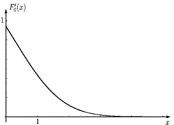
Hence, a=σ22p(0,0)2.169subscript𝑎superscript𝜎22subscriptsuperscript𝑝002.169a_{*}=\frac{\sigma^{2}}{2}p^{\prime}_{-}\left(0,0\right)\approx 2.169 and Π(dx)=xp(0,xy)λ+f+(y)𝑑ysubscriptΠ𝑑𝑥superscriptsubscript𝑥subscriptsuperscript𝑝0𝑥𝑦subscript𝜆subscript𝑓𝑦differential-d𝑦\Pi_{*}\left(dx\right)=\int_{x}^{\infty}p^{\prime}_{-}\left(0,x-y\right)\lambda_{+}f_{+}\left(y\right)dy can be expressed in terms of erf(x).erf𝑥\mathrm{erf}\left(x\right). Using formula (7), we can represent X+superscript𝑋X^{+} as the sum of a geometrically distributed number νG(1ρ),similar-to𝜈G1𝜌\nu\sim\mathrm{G}\left(1-\rho\right), exponentially distributed random variables ξ0,,ξn,Exp(c),similar-tosubscript𝜉0subscript𝜉𝑛Expsubscript𝑐\xi_{0},\ldots,\xi_{n},\ldots\sim\mathrm{Exp}\left(c_{*}\right), and random variables η1,,ηn,F,0\eta_{1},\ldots,\eta_{n},\ldots\sim F{}_{0}, where 1ρ0.418,1𝜌0.4181-\rho\approx 0.418, c1.104,subscript𝑐1.104c_{*}\approx 1.104, F0(x)dx=(Π(0,+))1Π(dx)subscriptsuperscript𝐹0𝑥𝑑𝑥superscriptsubscriptΠ01subscriptΠ𝑑𝑥F^{\prime}_{0}(x)dx=\left(\Pi_{*}\left(0,+\infty\right)\right)^{-1}\Pi_{*}\left(dx\right) (see Fig. 1). That is,

X+=ξ0+n=1ν(ξn+ηn).superscript𝑋subscript𝜉0superscriptsubscript𝑛1𝜈subscript𝜉𝑛subscript𝜂𝑛X^{+}=\xi_{0}+\sum_{n=1}^{\nu}\left(\xi_{n}+\eta_{n}\right).
Refer to caption
Figure 1: Density of ηisubscript𝜂𝑖\eta_{i}

References

  • [1] S. Asmussen, Applied Probability and Queues, Springer, New York, 2003.
  • [2] S. Asmussen, Ruin Probabilities, World Scientific, Singapore, 2010.
  • [3] A. E. Kyprianou, Introductory Lectures on Fluctuations of Levy Processes with Applications, Springer, New York, 2006.
  • [4] O. Kella, The class of distributions associated with the generalized Pollaczek–Khinchine formula, J. of Appl. Prob. 49(3) (2012), 883–887.
  • [5] M. Huzak et al., Ruin probabilities and decompositions for general perturbed risk processes, Annals of Appl Prob. 14 (2004), no. 3, 1378–1397.
  • [6] D. Gusak, On some generalization of the Pollaczek–Khinchine formula, Theory of Stoch. Process. 16(32) (2010), no. 1, 49–56.
  • [7] M. Kwasnicki, J. Malecki, and M. Ryznar, Suprema of Levy processes, Ann. of Probab. 41 (2013), no. 3B, 2047–2065.
  • [8] L. Chaumont, On the law of the supremum of Levy processes, Ann. of Probab. 41 (2013), no. 3A, 1191–1217.
  • [9] A. Kuznetsov, A. E. Kyprianou, J. C. Pardo, Meromorphic Levy processes and their fluctuation identities, Ann. of Appl. Prob. 22 (2012), no. 3, 1101–1135.
  • [10] N. Bratiychuk and D. Husak, Boundary-Values Problems for Processes with Independent Increments, Naukova Dumka, Kyiv, 1990 (in Russian).
  • [11] A. L. Lewis and E. Mordecki, Wiener-Hopf factorization for Levy processes having negative jumps with rational transforms, J. of Appl. Prob. 45 (2008), no. 1, 118–134.
  • [12] D. Husak, Processes with Independent Increments in Risk Theory, Institute of Mathematics of the NAS of Ukraine, Kyiv, 2011 (in Ukrainian).
  • [13] J. Bertoin, Levy Processes, Cambridge Univ. Press, Cambridge, 1996.
  • [14] E. Mordecki, Ruin probabilities for Levy processes with mixed-exponential negative jumps, Teor. Veroyatn. Primen., 48 (2003), 188–194.
  • [15] N. Cai and S. G. Kou, Option pricing under a mixed-exponential jump diffusion model, Manag. Sci. 57 (2011), no. 11, 2067–2081.