Conservation laws, exact travelling waves and modulation instability for an extended Nonlinear Schrödinger equation

Abstract.

We study various properties of solutions of an extended nonlinear Schrödinger (ENLS) equation, which arises in the context of geometric evolution problems – including vortex filament dynamics – and governs propagation of short pulses in optical fibers and nonlinear metamaterials. For the periodic initial-boundary value problem, we derive conservation laws satisfied by local in time, weak $H^{2}$ (distributional) solutions, and establish global existence of such weak solutions. The derivation is obtained by a regularization scheme under a balance condition on the coefficients of the linear and nonlinear terms – namely, the Hirota limit of the considered ENLS model. Next, we investigate conditions for the existence of traveling wave solutions, focusing on the case of bright and dark solitons. The balance condition on the coefficients is found to be essential for the existence of exact analytical soliton solutions; furthermore, we obtain conditions which define parameter regimes for the existence of traveling solitons for various linear dispersion strengths. Finally, we study the modulational instability of plane waves of the ENLS equation, and identify important differences between the ENLS case and the corresponding NLS counterpart. The analytical results are corroborated by numerical simulations, which reveal notable differences between the bright and the dark soliton propagation dynamics, and are in excellent agreement with the analytical predictions of the modulation instability analysis.

1. Introduction

1.1. The model and its physical significance

The present paper deals with an extended nonlinear Schrödinger (ENLS) equation, expressed in the following dimensionless form:

(1.1) $$\phi_{t}+3\alpha|\phi|^{2}\phi_{x}-{\rm i}\,\rho\,\phi_{xx}+\sigma\,\phi_{xxx}-{\rm i}\,\delta|\phi|^{2}\,\phi=0,$$

where $\phi(x,t)$ is the unknown complex field, subscripts denote partial derivatives, and $\alpha$, $\rho$, $\sigma$ and $\delta$ are real constants. Equation (1.1) has important applications in distinct physical and mathematical contexts. First, from the physical point of view, this model is one of the nonlinear dispersive equations which under the Hasimoto thransformation, $\phi(x,t)=\kappa(x,t)\,\exp\left({\rm i}\,\int_{0}^{x}\tau(\sigma,t)\,d\sigma\right)$ can be used to determine the motion of vortex filaments [16, 17, 25, 27, 33, 37, 44, 51]: here, the functions $\kappa(x,t)$ and $\tau(x,t)$ denote the curvature and torsion of the evolving filament, respectively, while $x$ represents length measured along the filament. When $\kappa(x,t)$ and $\tau(x,t)$ are specified, the shape of the filament as a curve is uniquely determined as it evolves in space [33].

It is crucial to remark that the derivation of (1.1) as an evolution equation for the Hasimoto transformation is valid only in the case where the coefficients $\alpha,\rho,\sigma,\delta$ satisfy the balance condition:

(1.2) $$\alpha\rho=\sigma\delta.$$

Then, Eq. (1.1) is known as Hirota equation [35], which is a combination of the nonlinear Schrödinger (NLS) and the Korteweg-de Vries (KdV) models: in particular, the NLS limit corresponds to the case $\alpha=\sigma=0$, while the complex modified KdV (cmKDV) limit corresponds to the case $\rho=\delta=0$. Note that the Hirota equation is a completely integrable model, belonging to the Ablowitz-Kaup-Newell-Segur (AKNS) hierarchy [1]. Its derivation in the context of the vortex filament motion is justified in [27, Sec. 3]. Briefly speaking, this derivation begins from a natural generalization of the localized induction equation (LIE) which governs the velocity of the vortex filament. The generalization takes account of the axial-flow effect up to the second-order (see [27, Eqs. (3.1)-(3.2)]). Then, the Hirota equation is derived by repeating the original Hasimoto’s procedure [33], which proved the equivalence between LIE and the integrable NLS equation $\mathrm{i}\phi_{t}+\phi_{xx}+\frac{1}{2}|\phi|^{2}\phi=0$ (see also [47, 48]). This equivalence implies that LIE is completely integrable. Thus, since the generalized LIE of [27] preserves integrability, the equivalent evolution equation which is in this case ENLS equation (1.1), should be also integrable. This is the reason why condition (1.2) is essential for the association of Eq. (1.1) with the vortex filament dynamics.

On the other hand, non-integrable versions of (1.1), i.e., when the balance condition (1.2) is violated, can be derived in the context of geometric evolution equations. In particular, it was shown in [53] that certain differential equations of one-dimensional dispersive flows into compact Riemann surfaces, may be reduced by a definition of a generalized Hasimoto transform, to ENLS type equations. See also [54, 55], and references therein.

Another important physical context, where certain versions of the ENLS equation have important applications, is that of nonlinear optics: such models have been used to describe femtosecond pulse propagation in nonlinear optical fibers; in such a case, $t$ and $x$ in Eq. (1.1) play, respectively, the role of the propagation distance along the optical fiber and the retarded time (in a reference frame moving with the group velocity), while $\phi(x,t)$ accounts for the (complex) electric field envelope. In the context of nonlinear fiber optics, the propagation of short optical pulses (of temporal width comparable to the wavelength) is accompanied by effects, such as higher-order (and, in particular, third-order) linear dispersion, as well as nonlinear dispersion (the latter is also called self-steepening term, due to its effect on the pulse envelope) [32]. These effects cannot be described within the framework of the standard NLS equation, but are taken into regard in Eq. (1.1): in the latter, the terms $\propto\phi_{xxx}$ and $|\phi|^{2}\phi_{x}$ account, respectively, for the third-order (linear) dispersion and self-steepening effects. Here, it should be noted that while the NLS equation is derived from Maxwell’s equations in the second-order of approximation in the reductive perturbation method (see, e.g., [32]), the above mentioned higher-order linear and nonlinear dispersion effects appear in the third-order of approximation, giving rise to ENLS-type equations, [8, 20, 24, 23, 31, 32, 36, 52, 58]. We also note that a similar situation occurs in the context of nonlinear metamaterials: in such media, propagation of ultrashort pulses (in the microwave of optical regimes) is also governed by various versions of ENLS models [59, 64, 67, 68].

The strong manifestation of the ENLS (1.1) in many applications, such as the ones mentioned above, motivates our study. This starts from basic analytical results concerning the derivation of conservation laws and global existence of weak solutions of (1.1), proceeds to the investigation of appropriate conditions for the existence of exact soliton solutions (in terms of bright and dark solitons), and finally addresses the modulational instability of plane waves, one of the fundamental mechanisms responsible for the generation of localized nonlinear structures [70].

1.2. Structure of the presentation and main findings

In Section 2, we focus on the global existence of $H^{2}$-weak solutions. The result concerns the ENLS (1.1) supplemented with periodic boundary conditions. The proof is based on the derivation of a differential equation for functionals, up to the level of the $H^{2}$-norm. We consider this differential equation for brevity, as an $H^{2}$-“energy equation” (borrowing the terminology of [6, 7] for relevant differential equations on functionals), and stress that it is not a conservation law. The main finding is that condition (1.2) is essential for the justification of the reduction of higher derivative terms, through a regularization and passage to the limit procedure leading to its rigorous derivation for weak solutions. In this regard, let us recall from the Sobolev embedding theorems, that weakly smooth $H^{m}(\mathbb{R})$- functions, for $m\geq 1$, are $C^{m-1}(\mathbb{R})$-smooth, and that the ENLS equation does not possess any smoothing effect. Furthermore, we identify an important difference form the NLS limit [65], related to additional implications on the application of the regularized approximation scheme, when the latter should be applied to the ENLS equation: in the case of the ENLS, we observe that in the passage to the limit, one has to deal with the appearance and handling of nonlinear multipliers, instead of the NLS-limit, where only linear multipliers are involved. For the global existence of weak solutions, the validity of the conservation of the Hamiltonian corresponding to the NLS-limit for weak solutions under the condition (1.2), as well as of the $L^{2}$-norm without any assumption on the coefficients is also crucial. While these conservation laws are known from earlier works [45], we revisit their derivation noting that the required formal computations are valid at least for solutions initiating from $H^{3}$-smooth initial data. However, we choose to work in the space of weak solutions $H^{3}$, only in order to simplify the presentation of the derivation of the conservation laws: comparing to the justification of the $H^{2}$-energy equation (relevant details are provided in Appendix A), the revision highlights that the conservation laws can be derived under weaker assumptions on the initial data –see Remark 2.6. This is a new result showing that conservation laws are valid even in the case of very weak assumptions on the smoothness of the initial conditions.

As a first application of the above results, we apply the $H^{2}$-energy equation to prove global existence of the weak solutions at the level of that norm, by combining it with appropriate alternative theorems [3]. It is interesting to recover that in addition to the balance condition (1.2), the presence of the second-order dispersion $\rho\neq 0$ is required, as a necessary condition for global existence.We note that the periodic case is in general quite different from the Cauchy case since dispersive effects are not expected (cf. [11]), and can lead even to blow-up phenomena in finite time for such types of equations, despite the fact that they may contain just cubic nonlinear terms (see [38] for a ENLS-type equation, and [71] on the periodic Dullin-Gottwald-Holm equation). Furthermore, our lines of approach are justified by the important outcomes of Kato’s theory [40]-[43], that the blow-up occurs in any $H^{k}$, $k\geq 2$-norm, if it occurs at all; see also [14]. The global well-posedness of the Cauchy problem for ENLS type equations in $H^{k}(\mathbb{R})$, $k\geq 2$ has been addressed in [50], with most recent results those of [39, 60] for the global well posedness for $1\leq k\leq 2$. We remark that the importance of the rigorous justification of conservation laws and energy equations has been also underlined in [5, 6, 7], and in [56] which considers the conservation laws for the Cauchy problem of the higher dimensional NLS equation.

In Section 3, we investigate conditions under which the ENLS (1.1) may support traveling wave solutions. The analysis is based on the reduction of (1.1) to an ordinary differential equation (ODE), by means of a traveling-wave ansatz. This method has been extensively used for the derivation of various types of traveling waves – such as periodic [26, 36], solitary [21, 36, 66] and unbounded [36, 66] ones – of the Hirota and other versions of the higher-other NLS model. We revisit the phase-plane analysis of the reduced dynamical system to obtain conditions for the existence of bright and dark solitons, as well as the solutions themselves. The main findings of this section (see also Remark 3.1) are the following. First, traveling solitons exist only under the balance condition (1.2). Second, we reveal the role of the wavenumber $k_{0}$ of the carrier wave: if $k_{0}\neq 0$ and $k_{0}\neq\rho/3\sigma$ traveling wave solutions exist only in the presence of both second ($\rho\neq 0$) and third-order ($\sigma\neq 0$) dispersion; if $k_{0}=0$ traveling waves may exist in both cases $\rho\neq 0$ and $\rho=0$, corresponding to the so-called “zero-dispersion point” (ZDP) in the context of nonlinear fiber optics [4]. Note that in the ZDP case, we find that the carrier frequency should also vanish, in which case the balance condition (1.2) yields $\delta=0$, and the ENLS (1.1) becomes the cmKdV model. This way, we also elucidate the importance of the linear dispersion effect on the existence of soliton solutions. Third, yet another interesting finding is that standing wave solutions are not supported by the ENLS (1.1).

We also present results of direct numerical simulations illustrating that, when (1.2) is satisfied, the solitons are robust under small-amplitude random-noise perturbations. On the other hand, when (1.2) is violated, our numerical results illustrate that an arbitrary initial solitary pulse is always followed by emission of radiation (which tends to disperse at later times. The results on the robustness of the solitons, as well as on the radiation emission when (1.2) is violated, are in accordance to the findings of Ref. [31] and the analysis of [57, 69], which refer to the case of the bright solitons. However, the numerical simulations also reveal important differences, regarding the dynamics of bright and dark pulses. For instance, regarding the emission of radiation, we find that a dark solitary wave initial condition tends to a single dark pulse, which is eventually separated by the emitted radiation; the latter, is traveling faster from the soliton, and assumes the form of an apparent dispersive shock wave [34]. On the contrary, in the case of a bright solitary wave the radiation arises behind the principal pulse. Another important difference concerns the direction of the propagation of the pulses: while the evolution of bright solitons is associated with a turning effect – i.e., the soliton initially starts moving towards the positive $x$-direction, but eventually travels with an almost constant velocity towards the negative $x$-direction – this effect is not observed in the evolution of the dark soliton. This effect for the bright solitary wave structures is somewhat reminiscent of direction-reversing solitary waves, so-called “boomerons”; see, e.g., Ref. [19] and references therein. We note that all numerical experiments have been performed by using a pseudo-spectral method, under which the numerical quantities related to the conservation laws of the ENLS equation under the balance condition (1.2), are also conserved at a high order of accuracy.

In Section 4, we perform a modulation instability (MI) analysis of plane wave solutions of (1.1). Here, we should recall that MI is the process by which a plane wave of the form $\phi(x,t)=\phi_{0}\mathrm{e}^{\mathrm{i}(kx-\omega t)}$, $\phi_{0}\in\mathbb{R}$, becomes unstable and gives rise to the emergence of nonlinear structures [70]. One of the main findings of the MI analysis, is the detection of the drastic differences between the conditions for MI on the ENLS equation (1.1) and its NLS-limit; in particular, we find the following. If the wavenumber of the plane wave solution is $k=0$ then the MI conditions for the focusing counterpart of the ENLS equation (3.12) are exactly the same with its focusing NLS-limit. Additionally, the plane waves are always modulationally stable in the defocusing ENLS equation, as it happens in its defocusing NLS-limit. On the other hand, when $k\neq 0$, we reveal MI conditions for both the focusing and the defocusing counterparts of the ENLS equation that are clearly distinct from their NLS counterparts. Specifically, the MI conditions in the focusing case are similar to those of the focusing NLS-limit but the instability band may decrease or increase depending on the values of the parameters involved; on the other hand, we find that in the defocusing case of the ENLS equation, MI may be manifested. This is a drastic difference with the defocusing NLS limit where the plane waves are always stable. The analytical considerations of the MI analysis are concluded by the justification that, in the MI regime, the Fourier modes of the unstable plane wave solution are the integer multiples of the unstable wave number of the perturbation (the well known “sidebands” pertaining to the MI). The results of the numerical studies are in excellent agreement with the analytical predictions of the MI analysis.

Finally, Section 5 offers a discussion and a summary of our results, and discusses some future directions.

2. Conservation laws and global existence of solutions

In this section, we consider the derivation of conservation laws and energy-type equations for the ENLS equation (1.1). These quantities will have a crucial role in proving global existence of weak solutions, for the periodic initial-boundary value problem of this equation. More precisely, we supplement the ENLS equation (1.1) with space-periodic boundary conditions,

(2.1) $$\phi(x+L,t)=\phi(x,t),\quad\forall\,x\in{\mathbb{R}},\;\;\forall\,t\in{\mathbb{R}},$$

where $L>0$ is given, and with the initial condition

(2.2) $$\phi(x,0)=\phi_{0}(x),\;\;\forall\,x\in{\mathbb{R}}.$$

Let us recall some preliminary information on the functional setting of the problem, as well as a local existence result. Problem (1.1)-(2.1)-(2.2) will be considered in complexifications of the Sobolev spaces $H^{m}_{per}(\Omega)$ of real periodic functions, locally in $H^{m}(\mathbb{R})$, where $m$ is a nonnegative integer and $\Omega=(0,L)$. These spaces $H^{m}_{per}(\Omega)$ are endowed with the scalar product and the induced from it norm, given below

(2.3) $$(\phi,\psi)_{\scriptscriptstyle H^{m}(\Omega)}:=\sum_{j=0}^{m}\int_{\scriptscriptstyle\Omega}\partial^{j}\phi\,\partial^{j}\overline{\psi}\;dx\quad\text{\rm and}\quad\|\phi\|_{\scriptscriptstyle H^{m}(\Omega)}:=\sqrt{(\phi,\phi)_{m}},$$

where $\partial^{j}:=\frac{\partial^{j}}{\partial x^{j}}$. The case $m=0$, simply corresponds to $L^{2}(\Omega)$. The spaces $H^{m}_{per}(\Omega)$ can be studied by using Fourier series expansion, and they can be characterized as

$$H^{m}_{per}(\Omega)=\left\{\sum_{k\in\mathbb{Z}}\widehat{\phi}_{k}\,\mathrm{e}^{{\rm 2\pi i}\,\frac{k}{L}\,x}:\quad\widehat{\phi}_{k}=\overline{{\widehat{\phi}}_{-k}}\quad\forall\,k\in{\mathbb{Z}},\quad\sum_{k\in\mathbb{Z}}(1+|k|^{2})^{m}\,|\widehat{\phi}_{k}|^{2}<\infty\right\},$$

where $\widehat{\phi}_{k}=\overline{\widehat{\phi}_{-k}}$ are the (real) Fourier coefficients [22]. The scalar product and the norm in $H^{m}_{per}(\Omega)$ given by (2.3), are equivalent to those defined in terms of Fourier coefficients

(2.4) $$(\phi,\psi)_{m,*}=\sum_{k\in\mathbb{Z}}(1+|k|^{2})^{m}\,\widehat{\phi}_{k}\,\widehat{\psi}_{k}\quad\text{\rm and}\quad\|\phi\|_{m,*}=\left[\,\sum_{k\in\mathbb{Z}}(1+|k|^{2})^{m}\,|\widehat{\phi}_{k}|^{2}\right]^{\frac{1}{2}},$$

i.e., there exist constants $c_{1},c_{2}>0$ such that

(2.5) $$c_{1}\,\|\phi\|_{\scriptscriptstyle H^{m}(\Omega)}\,\leq\,\|\phi\|_{m,*}\,\leq\,c_{2}\,\|\phi\|_{\scriptscriptstyle H^{m}(\Omega)}.$$

The complexified space of $H^{m}_{per}(\Omega)$ becomes a real Hilbert space, (which shall be still denoted for convenience by $H^{m}_{per}(\Omega)$), if it is endowed with the inner product and norm

(2.6) $$\begin{gathered}{[}\phi,\psi]_{\scriptscriptstyle H^{m}(\Omega)}:=\mathrm{Re}\left[\,\sum_{j=0}^{m}\int_{\scriptscriptstyle\Omega}\partial^{j}\phi\,\partial^{j}\overline{\psi}\;dx\,\right]=(\phi_{1},\psi_{1})_{\scriptscriptstyle H^{m}(\Omega)}+(\phi_{2},\psi_{2})_{\scriptscriptstyle H^{m}(\Omega)},\\ \|\phi\|_{\scriptscriptstyle H^{m}(\Omega)}:=\sqrt{[\phi,\phi]_{\scriptscriptstyle H^{m}(\Omega)}},\end{gathered}$$

where $\phi=\phi_{1}+{\rm i}\,\phi_{2}$ and $\psi=\psi_{1}+{\rm i}\,\psi_{2}$. The equivalent norms in terms of Fourier coefficients are defined, taking into account (2.4) and (2.5), in an analogous manner to (2.6).

For $m\geq 1$, the following embedding relations

(2.7) $$H^{m}_{per}(\Omega)\subseteq C^{m-1}(\Omega),\quad H^{m}_{per}(\Omega)\subseteq H^{m-1}_{per}(\Omega),$$

are compact. Moreover $H^{m}_{per}(\Omega)$ is a generalized Banach algebra: there exists a constant $c$ depending only on $\Omega$, such that if $z,\,\eta\in H^{m}_{per}(\Omega)$, then $z\cdot\eta\in H^{m}_{per}(\Omega)$ and

(2.8) $$\|z\cdot\eta\|_{\scriptscriptstyle H^{m}(\Omega)}\leq\,c\,\|z\|_{\scriptscriptstyle H^{m}(\Omega)}\,\|\eta\|_{\scriptscriptstyle H^{m}(\Omega)}.$$

We also recall the Gagliardo-Nirenberg inequality for the one space dimension case. Let $\Omega\subseteq{\mathbb{R}}$, $1\leq p,q,r\leq\infty$, $j$ an integer, $0\leq j\leq m$ and $\frac{j}{m}\leq\theta\leq 1$. Then

(2.9) $$\|\partial^{j}\phi\|_{\scriptscriptstyle L^{p}(\Omega)}\leq\,C\,\|\phi\|^{1-\theta}_{\scriptscriptstyle L^{q}(\Omega)}\,\left(\,\sum^{m}_{k=0}\|\partial^{k}\phi\|_{\scriptscriptstyle L^{r}(\Omega)}\,\right)^{\theta},\quad\forall\,\phi\in L^{q}(\Omega)\cap W^{m,r}(\Omega),$$

where $\frac{1}{p}=j+\theta\left(\frac{1}{r}-m\right)+\frac{1-\theta}{q}$. If $m-j-\frac{1}{r}=0$ and $r>1$, then the inequality holds for $\theta<1$.

One of the methods which can be used in order to prove a local existence result, is the method of semibounded evolution equations which was developed in [42]. The application of this method to (2.16)-(2.2)-(2.1) although involving lengthy computations, is now considered as standard. Thus, we refrain to show the details here, and we just state the local existence result in

Theorem 2.1.

Let $\phi_{0}\in H^{k}_{per}(\Omega)$ for any integer $k\geq 2$, and $\alpha,\rho,\sigma,\delta\in\mathbb{R}$. Then there exists $T>0$, such that the problem (1.1)-(2.1)-(2.2), has a unique solution

$$\phi\in C([0,T],H^{k}_{per}(\Omega))\quad\mbox{and}\quad\phi_{t}\in C([0,T],H^{k-3}_{per}(\Omega)).$$

Remark 2.2.

(Generalized equation). Except for the method of [41, 42], a modification of the methods for local existence of solutions for nonlinear hyperbolic systems is applicable to the generalized ENLS equation,

(2.10) $$\phi_{t}+\beta(|\phi|^{2})\,\phi_{x}-{\rm i}\,\rho\,\phi_{xx}+\sigma\,\phi_{xxx}-{\rm i}\,\gamma(|\phi|^{2})\,\phi=0\quad\text{\rm on}\quad{\mathbb{R}}\times(0,T],$$

where the given functions

(2.11) $$\beta,\gamma\in C^{1}({\mathbb{R}};{\mathbb{R}}).$$

For instance, it can be proved in a similar manner (see also [62, Theorem 1.2, pg. 362 & Proposition 1.3, pg. 364]), that if $\phi_{0}\in H^{k}_{per}(\Omega)$, $k\geq 2$, then $\phi\in C([0,T],H^{k}_{per}(\Omega))$. Note that the problem does not possess, a-priori, any smoothing effect. Moreover, the arguments of [41, 42, 62], imply continuous dependence on initial data in $H^{k}_{per}(\Omega)$.

It is known (see, e.g., Ref. [45]), that solutions of the problem (1.1)-(2.2)-(2.1) possess conservation laws similar to the conservation of the $L^{2}$-norm and energy as the the solutions of its NLS-limit, i.e. the quantities

(2.12) $$\mathbf{N}(\phi):=\int_{\scriptscriptstyle\Omega}|\phi|^{2}\;dx=\|\phi\|^{2}_{\scriptscriptstyle L^{2}(\Omega)},$$

(2.13) $$\mathbf{J}(\phi):=\tfrac{\rho}{2}\,\int_{\scriptscriptstyle\Omega}|\phi_{x}|^{2}\;dx-\tfrac{\delta}{4}\,\int_{\scriptscriptstyle\Omega}|\phi|^{4}\;dx.$$

are conserved. Notice that while the first $L^{2}$ norm is conserved for all parameter combinations, the second conservation law only holds if Eq. (1.2) is satisfied. Here, first we briefly discuss their derivation, in the case of sufficiently smooth initial data, with the regularity suggested by Theorem 2.1 for $k=3$; nevertheless, below we extend our considerations and show that the conservation laws are satisfied by weak solutions, even when the latter are initiating for considerably weak initial data, belonging to an appropriate class of Sobolev spaces (cf. Remark 2.6 below).

Hence, assuming $H^{3}$-smoothness of the initial data, we recall the following

Lemma 2.3.

For $\phi_{0}\in H^{3}_{per}(\Omega)$, let $T^{*}$ be the maximum time for which for all $0<T<T^{*}$, the solution $\phi$ of (1.1)-(2.1)-(2.2) lies in $C([0,T],H^{3}_{per}(\Omega))\cap C^{1}([0,T],L^{2}(\Omega))$. Then for any $t\in[0,T^{*})$, the solution satisfies the conservation law

(2.14) $$\mathbf{N}(\phi(t))=\mathbf{N}(\phi_{0}),$$

for all $\alpha,\rho,\sigma,\delta\in\mathbb{R}$. Furthermore, if (1.2) is satisfied, then the NLS Hamiltonian is conserved, that is,

(2.15) $$\mathbf{J}(\phi(t))=\mathbf{J}(\phi_{0}).$$

Proof.

For convenience, we rewrite equation (1.1) as

(2.16) $$\phi_{t}-{\rm i}\,\rho\,\phi_{xx}+\sigma\,\phi_{xxx}=-3\alpha\,|\phi|^{2}\phi_{x}+{\rm i}\,\delta\,|\phi|^{2}\phi.$$

Since $\phi\in C([0,T],H^{3}_{per}(\Omega))\cap C^{1}([0,T],L^{2}(\Omega))$, it makes sense to multiply equation (2.16) by $\overline{\phi}$, integrate with respect to space and keep real parts. We obtain the equation

(2.17) $$\tfrac{1}{2}\,\tfrac{d}{dt}\|\phi(t)\|^{2}_{\scriptscriptstyle L^{2}(\Omega)}+\tfrac{3\alpha}{2}\,\mathrm{Re}\left[\,\int_{\scriptscriptstyle\Omega}|\phi|^{2}(|\phi|^{2})_{x}\;dx\,\right]+\sigma\mathrm{Re}\left[\,\int_{\scriptscriptstyle\Omega}\phi_{xxx}\overline{\phi}\;dx\right]=0.$$

By periodicity, the last two integrals vanish, and (2.14) follows.

To derive the conservation law (2.15), we multiply (2.16) by $\overline{\phi}_{t}$, integrate in space, keeping this time the imaginary parts. Now, the resulting equation is

(2.18) $$\tfrac{d}{dt}J(\phi(t))+3\,\alpha\,\mathrm{Im}\left[\,\int_{\scriptscriptstyle\Omega}|\phi|^{2}\,\phi_{x}\overline{\phi}_{t}\;dx\,\right]+\sigma\,\mathrm{Im}\left[\int_{\scriptscriptstyle\Omega}\phi_{xxx}\,\overline{\phi}_{t}\;dx\,\right]=0.$$

By substitution of $\overline{\phi}_{t}=-\mathrm{i}\rho\overline{\phi}_{xx}-\sigma\overline{\phi}_{xxx}-3\alpha|\phi|^{2}\overline{\phi}_{x}-\mathrm{i}\delta|\phi|^{2}\overline{\phi}$, into the two integral terms of the left-hand side of (2.18), and integration by parts, we observe that these two terms become:

(2.19) $$\begin{split}3\,\alpha\,\mathrm{Im}\left[\int_{\scriptscriptstyle\Omega}|\phi|^{2}\,\phi_{x}\,\overline{\phi}_{t}\;dx\right]=&3\,\alpha\,\mathrm{Im}\left[\int_{\scriptscriptstyle\Omega}|\phi|^{2}\,\phi_{x}\left(-3\,\alpha\,|\phi|^{2}\,\overline{\phi}_{x}-{\rm i}\,\rho\,\overline{\phi}_{xx}-\sigma\,\overline{\phi}_{xxx}-{\rm i}\,\delta\,|\phi|^{2}\,\overline{\phi}\right)\;dx\right]\\ =&-3\,\alpha\,\rho\mathrm{Re}\left[\int_{\scriptscriptstyle\Omega}|\phi|^{2}\,\phi_{x}\,\overline{\phi}_{xx}\;dx\right]-3\,\alpha\,\sigma\,\mathrm{Im}\left[\int_{\scriptscriptstyle\Omega}|\phi|^{2}\,\phi_{x}\,\overline{\phi}_{xxx}\;dx\right],\\ &-\tfrac{3\alpha\rho}{2}\,\left[\int_{\scriptscriptstyle\Omega}|\phi|^{2}\,(|\phi_{x}|^{2})_{x}\;dx\right]+3\,\alpha\,\sigma\,\mathrm{Im}\left[\int_{\scriptscriptstyle\Omega}|\phi|^{2}\,\overline{\phi}_{x}\,\phi_{xxx}\;dx\right],\end{split}$$

and

(2.20) $$\sigma\,\mathrm{Im}\left[\int_{\scriptscriptstyle\Omega}\phi_{xxx}\,\overline{\phi}_{t}\;dx\right]=-\sigma\,\delta\,\mathrm{Re}\left[\int_{\scriptscriptstyle\Omega}|\phi|^{2}\,\phi_{xxx}\,\overline{\phi}\;dx\right]-3\,\alpha\,\sigma\,\mathrm{Im}\left[\int_{\scriptscriptstyle\Omega}|\phi|^{2}\,\overline{\phi}_{x}\,\phi_{xxx}\;dx\right].$$

Then, by using (2.19) and (2.20), equation (2.18) can be written as

(2.21) $$\tfrac{d}{dt}J(\phi(t))-\tfrac{3\alpha\rho}{2}\,\left[\int_{\scriptscriptstyle\Omega}|\phi|^{2}\,(|\phi_{x}|^{2})_{x}\;dx\right]-\sigma\,\delta\,\mathrm{Re}\left[\int_{\scriptscriptstyle\Omega}|\phi|^{2}\,\phi_{xxx}\,\overline{\phi}\;dx\right]=0.$$

For the last term of the left-hand side of (2.21), we observe that

(2.22) $$-\sigma\,\delta\,\mathrm{Re}\left[\int_{\scriptscriptstyle\Omega}|\phi|^{2}\,\phi_{xxx}\,\overline{\phi}\;dx\right]=\tfrac{\sigma\delta}{2}\,\left[\int_{\scriptscriptstyle\Omega}|\phi|^{2}\,(|\phi_{x}|^{2})_{x}\;dx\right]+\sigma\,\delta\,\mathrm{Re}\left[\int_{\scriptscriptstyle\Omega}\phi_{xx}\,\overline{\phi}\,(|\phi|^{2})_{x}\;dx\right],$$

while for the last term of the right-hand side of (2.22),

(2.23) $$\sigma\,\delta\,\mathrm{Re}\left[\int_{\scriptscriptstyle\Omega}\phi_{xx}\,\overline{\phi}\,(|\phi|^{2})_{x}\;dx\right]=\tfrac{\sigma\delta}{2}\,\left[\int_{\scriptscriptstyle\Omega}|\phi|^{2}\,(|\phi_{x}|^{2})_{x}\;dx\right]+\sigma\,\delta\,\mathrm{Re}\left[\int_{\scriptscriptstyle\Omega}\phi_{xx}\,\phi_{x}\,\overline{\phi}^{2}\;dx\right].$$

Also, for the last term of the right hand side of (2.23), we have

$$\begin{split}\sigma\,\delta\,\mathrm{Re}\left[\int_{\scriptscriptstyle\Omega}\phi_{xx}\,\phi_{x}\,\overline{\phi}^{2}\;dx\right]=&-\,\sigma\,\delta\,\mathrm{Re}\left[\int_{\scriptscriptstyle\Omega}\phi_{x}\,\left(\phi_{xx}\,\overline{\phi}^{2}+2\,\phi_{x}\overline{\phi}\,\overline{\phi}_{x}\right)\;dx\right]\\ =&-\,\sigma\,\delta\,\mathrm{Re}\left[\int_{\scriptscriptstyle\Omega}\phi_{xx}\,\phi_{x}\,\overline{\phi}^{2}\,dx\right]-2\,\sigma\,\delta\,\mathrm{Re}\left[\int_{\scriptscriptstyle\Omega}|\phi_{x}|^{2}\,\phi_{x}\,\overline{\phi}\,dx\right].\end{split}$$

Hence, we have for this term, that

(2.24) $$\begin{split}\sigma\,\delta\,\mathrm{Re}\left[\int_{\scriptscriptstyle\Omega}\phi_{xx}\,\phi_{x}\,\overline{\phi}^{2}\;dx\right]=&-\,\sigma\,\delta\,\mathrm{Re}\left[\int_{\scriptscriptstyle\Omega}|\phi_{x}|^{2}\,\phi_{x}\,\overline{\phi}\,dx\right]\\ =&-\tfrac{\sigma\delta}{2}\,\left[\int_{\scriptscriptstyle\Omega}(|\phi|^{2})_{x}\,|\phi_{x}|^{2}\;dx\right]=\tfrac{\sigma\delta}{2}\,\left[\int_{\scriptscriptstyle\Omega}|\phi|^{2}\,(|\phi_{x}|^{2})_{x}\;dx\right].\end{split}$$

Eventually, it follows from (2.22)-(2.24), that the last term of (2.21) is

(2.25) $$-\sigma\,\delta\,\mathrm{Re}\left[\int_{\scriptscriptstyle\Omega}|\phi|^{2}\,\phi_{xxx}\,\overline{\phi}\;dx\right]=\tfrac{3\delta\sigma}{2}\,\mathrm{Re}\left[\int_{\scriptscriptstyle\Omega}|\phi|^{2}\,(|\phi_{x}|^{2})_{x}\;dx\right].$$

Therefore, equation (2.21) is taking the form

(2.26) $$\tfrac{d}{dt}J(\phi(t))=\tfrac{3}{2}(\alpha\rho-\sigma\delta)\,\left[\int_{\scriptscriptstyle\Omega}|\phi|^{2}\,(|\phi_{x}|^{2})_{x}\;dx\right]=-\tfrac{3}{2}(\alpha\rho-\sigma\delta)\,\left[\int_{\scriptscriptstyle\Omega}(|\phi|^{2})_{x}\,|\phi_{x}|^{2}\;dx\right].$$

The assumption (1.2) on the coefficients, shall be used on the equation (2.26), implies that $\frac{d}{dt}\,J(\phi(t))=0$, i.e., the conservation law (2.15). ∎

The conservation laws provided by Lemma 2.3 will be useful in order to establish global in time regularity for the solutions of (1.1)-(2.2)-(2.1), at $H^{2}_{per}(\Omega)$-level. For this purpose, we derive a differential equation for functionals involving 2nd-order derivatives. For brevity, we call this differential equation as “energy equation” (as per the terminology used in Refs. [6, 7]), but stressing that it is not a conservation law.

Lemma 2.4.

For $\phi_{0}\in H^{3}_{per}(\Omega)$, let $T^{*}$ be the maximum time for which for all $0<T<T^{*}$, the solution $\phi$ of (1.1)-(2.1)-(2.2), lies in $C([0,T],H^{3}_{per}(\Omega))\cap C^{1}([0,T],L^{2}(\Omega))$. Moreover, assume that the coefficients satisfy (1.2). We consider the functionals

(2.27) $$\mathbf{J_{1}}(\phi):=\rho\,\int_{\scriptscriptstyle\Omega}|\phi_{xx}|^{2}\;dx-4\,\delta\,\left[\int_{\scriptscriptstyle\Omega}|\phi|^{2}\,|\phi_{x}|^{2}\;dx\right]-\delta\,\mathrm{Re}\left[\int_{\scriptscriptstyle\Omega}\phi^{2}\,\overline{\phi}^{2}_{x}\;dx\right],$$

and

(2.28) $$\begin{split}\mathbf{E_{1}}(t):=&\,9\,\alpha\,\delta\,\left[\int_{\scriptscriptstyle\Omega}|\phi|^{2}\,|\phi_{x}|^{2}\,(|\phi|^{2})_{x}\;dx\right]-6\,\alpha\,\delta\,\mathrm{Re}\left[\int_{\scriptscriptstyle\Omega}|\phi|^{2}\,\phi_{x}\,\overline{\phi}^{2}\,\phi_{xx}\;dx\right]\\ &\,-8\,\delta\,\rho\,\mathrm{Im}\left[\int_{\scriptscriptstyle\Omega}|\phi|^{2}\,\phi\,\overline{\phi}_{xx}\;dx\right]-4\,\delta\,\rho\,\mathrm{Im}\left[\int_{\scriptscriptstyle\Omega}|\phi_{x}|^{2}\,\overline{\phi}\,\phi_{xx}\;dx\right]\\ &\,+6\,\delta^{2}\,\mathrm{Im}\left[\int_{\scriptscriptstyle\Omega}|\phi|^{4}\,\overline{\phi}\,\phi_{xx}\;dx\right]-6\,\delta^{2}\,\int_{\scriptscriptstyle\Omega}|\phi|^{2}\,\phi^{2}\overline{\phi}_{x}\;dx.\\ \end{split}$$

Then the solution $\phi$, for any $t\in[0,T]$ satisfies the energy equation

(2.29) $$\tfrac{d}{dt}\,\mathbf{J_{1}}(\phi)=\mathbf{E_{1}}(t).$$

Proof.

An attempt for the formal derivation of (2.29) readily reveals the generation of higher order derivative terms, on which, direct calculations are not permitted by the weak regularity assumptions on the initial data. Therefore, we shall rigorously calculate the time-derivative of the functional (2.27) (as suggested by the right-hand side of the claimed equation (2.29)), by following an approximation scheme (close to that developed in [65] for the linearly damped and forced NLS equation). The scheme is based on a smooth approximation of the solution of (1.1)-(2.2)-(2.1), both in space and time. We denote by

(2.30) $$\left<\phi,\psi\right>_{H^{m},H^{-m}}=\mathrm{Re}\left[\int_{\scriptscriptstyle\Omega}\phi\,\psi\;dx\right],$$

the duality bracket between the space $H^{m}$ and its dual $H^{-m}$, $m\geq 1$, to elucidate that several quantities act as functionals during our calculations. Note also that due to the (compact) embeddings $H^{m}_{per}(\Omega)\subset L^{2}(\Omega)\subset H^{-m}_{per}(\Omega)$, $m\geq 1$, the identification

(2.31) $$\left<\phi,\psi\right>_{H^{m},H^{-m}}=(\phi,\psi)_{\scriptscriptstyle L^{2}(\Omega)},\quad\mbox{for every}\quad\phi\in H^{m}_{per}(\Omega),\quad\psi\in L^{2}(\Omega),$$

holds.

For the smooth approximation in space, we consider for arbitrary $n\in\mathbb{N}$, the low frequency part of the unique solution $\phi\in C([0,T],H^{3}_{per}(\Omega))\cap C^{1}([0,T],L^{2}(\Omega))$ of (1.1)-(2.2)-(2.1),

(2.32) $$\phi_{n}(t)=\sum_{|k|\leq n}\widehat{\phi}_{k}(t)\,\mathrm{e}^{{\rm 2\pi i}\,\frac{k}{L}\,x},$$

which is the projection of the solution $\phi$ onto the first $n$ Fourier modes. The function $\phi_{n}$ is a smooth analytic function with respect to the space variable. A regularization of $\phi_{n}$ in time, can be obtained by a standard mollification in time. For instance, we consider the standard mollifier in time $J_{\epsilon}(t)=\epsilon^{-1}J(t/\epsilon)$, $\epsilon>0$, with the properties $J_{\epsilon}(t)=0$ if $|t|\geq\epsilon$, and $\int_{\scriptscriptstyle\mathbb{R}}J_{\epsilon}(t)dt=1$. Recall that $J\in C_{0}^{\infty}(\mathbb{R})$, $J\geq 0$ on $\mathbb{R}$, and $\int_{\scriptscriptstyle\mathbb{R}}J(x)dx=1$. Then, the function

$$J_{\epsilon}*\phi_{n}\,(t)=\int_{\scriptscriptstyle\mathbb{R}}J_{\epsilon}(t-s)\phi_{n}(s)ds,$$

is infinitely differentiable function on $\mathbb{R}$ into $H^{3}_{per}(\Omega)$. Furthermore, by setting $\epsilon=\frac{1}{n}$, we see that the regularized sequence $v_{n}=J_{\frac{1}{n}}*\phi_{n}$, satisfies the key convergence relations to $\phi\in L^{2}([0,T],X)$, $X=H^{m}_{per}(\Omega)$, $-2\leq m\leq 3$, given in (A.2) –cf. Appendix A.

We indicatively demonstrate the calculations required for the time derivative $\tfrac{d}{dt}\left(|\phi_{x}|^{2},|\phi|^{2}\right)_{\scriptscriptstyle L^{2}(\Omega)}$-the time derivative of the second term of of the functional (2.27). We note again that more details can be found in Appendix A. By using the approximating sequence $v_{n}$, Lemmas A.1 and A.2, and performing the calculations for $v_{n}$ in the sense of the dual spaces as in (A.3), we derive the equation

(2.33) $$\begin{split}\left(|v_{nx}(t)|^{2},|v_{n}(t)|^{2}\right)_{\scriptscriptstyle L^{2}(\Omega)}-\left(|v_{nx}(0)|^{2},|v_{n}(0)|^{2}\right)_{\scriptscriptstyle L^{2}(\Omega)}=&-2\int_{0}^{t}\left<|v_{n}|^{2}\overline{v}_{nxx},v_{nt}\right>_{\scriptscriptstyle H^{1},H^{-1}}\;d\tau\\ &-2\int_{0}^{t}\left<\overline{v}_{nx}^{2}v_{n},v_{nt}\right>_{\scriptscriptstyle H^{2},H^{-2}}d\tau,\end{split}$$

which holds for every $t\in[0,T]$. A difference from the NLS equation [65], is that in the passage to the limit to (2.33) (or its equivalent (A.3)), we have to deal with the appearance of nonlinear multipliers in the right-hand side. We first observe that by using (A.2) and Aubin-Lions [61, Corollary 4, p.85], we may derive the strong convergence

(2.34) $$\begin{array}[]{lllll}v_{n}&\rightarrow&\phi,&\mbox{in}&L^{2}([0,T],H^{2}_{per}(\Omega)),\\ v_{nxx}&\rightarrow&\phi_{txx},&\mbox{in}&L^{2}([0,T],L^{2}(\Omega)).\end{array}$$

On the other hand, we may see that there exists some $c>0$ such that

$$\int_{0}^{\scriptscriptstyle T}\|\,|v_{n}|^{2}{v}_{nxx}-|\phi|^{2}{\phi}_{xx}\,\|_{\scriptscriptstyle L^{2}(\Omega)}^{2}\,ds\leq\,c\,\left\{\int_{0}^{\scriptscriptstyle T}\|{v}_{nxx}-\phi_{xx}\|^{2}_{\scriptscriptstyle L^{2}(\Omega)}\;ds+\int_{0}^{\scriptscriptstyle T}\|{v}_{n}-\phi\|^{2}_{\scriptscriptstyle L^{2}(\Omega)}\;ds\right\}\rightarrow 0,$$

as $n\rightarrow\infty$; the second term in the right hand side of (2.33) may be treated similarly. Letting $n\rightarrow\infty$, equation (2.33) (or (A.3)) converges to

(2.35) $$\tfrac{d}{dt}\left(|\phi_{x}|^{2},|\phi|^{2}\right)_{\scriptscriptstyle L^{2}(\Omega)}=-2\left<|\phi|^{2}\overline{\phi}_{xx},\phi_{t}\right>_{\scriptscriptstyle H^{1},H^{-1}}-2\left<\overline{\phi}_{x}^{2}\phi,\phi_{t}\right>_{\scriptscriptstyle H^{2},H^{-2}}.$$

From (2.35), we may proceed by inserting the expression for $\phi_{t}$ provided by (2.16). Manipulating the right-hand side of (2.35) as shown in (A.4), we derive the equation (A.5), which is valid for the solution $\phi\in C([0,T],H^{3}_{per}(\Omega))$, since it only contains (weak) derivatives up to the third order. This fact allows for further integration by parts to the right-hand side of (A.5). Eventually, we arrive in

(2.36) $$\begin{split}\tfrac{d}{dt}\int_{\scriptscriptstyle\Omega}|\phi|^{2}\,|\phi_{x}|^{2}\;dx=&\,3\,\alpha\,\mathrm{Re}\left[\int_{\scriptscriptstyle\Omega}|\phi|^{4}\,(|\phi_{x}|^{2})_{x}\;dx\right]+3\,\sigma\,\mathrm{Re}\left[\int_{\scriptscriptstyle\Omega}|\phi|^{2}\,(|\phi_{xx}|^{2})_{x}\;dx\right]\\ &+3\,\alpha\,\mathrm{Re}\left[\int_{\scriptscriptstyle\Omega}|\phi|^{2}\,|\phi_{x}|^{2}\,(|\phi|^{2})_{x}\;dx\right]+2\,\delta\,\mathrm{Im}\left[\int_{\scriptscriptstyle\Omega}|\phi|^{4}\,\phi\,\overline{\phi}_{xx}\;dx\right]\\ &+2\,\rho\,\mathrm{Im}\left[\int_{\scriptscriptstyle\Omega}\overline{\phi}_{x}^{2}\,\phi\,\phi_{xx}\;dx\right]+2\,\delta\,\mathrm{Im}\left[\int_{\scriptscriptstyle\Omega}\overline{\phi}_{x}^{2}\,\phi^{2}\,|\phi|^{2}\;dx\right].\\ \end{split}$$

For the time derivatives of the rest of the terms of (2.27), we work similarly (see Appendix A): for the first term, the derivative is

(2.37) $$\begin{split}\tfrac{d}{dt}\int_{\scriptscriptstyle\Omega}|\phi_{xx}|^{2}dx=&\,12\,\alpha\,\mathrm{Re}\left[\int_{\scriptscriptstyle\Omega}|\phi|^{2}\,(|\phi_{xx}|^{2})_{x}\;dx\right]-6\,\alpha\,\mathrm{Re}\left[\int_{\scriptscriptstyle\Omega}\overline{\phi}_{xx}^{2}\,\phi_{x}\,\phi\;dx\right]\\ &-8\,\delta\,\mathrm{Im}\left[\int_{\scriptscriptstyle\Omega}|\phi_{x}|^{2}\,\phi\,\overline{\phi}_{xx}\;dx\right]-4\,\delta\,\mathrm{Im}\left[\int_{\scriptscriptstyle\Omega}\phi_{x}^{2}\,\overline{\phi}_{xx}\,\overline{\phi}\;dx\right]\\ &-2\,\delta\,\mathrm{Im}\left[\int_{\scriptscriptstyle\Omega}\phi^{2}\,\overline{\phi}_{xx}^{2}\;dx\right],\\ \end{split}$$

and for the third term,

(2.38) $$\begin{split}\tfrac{d}{dt}\int_{\scriptscriptstyle\Omega}\phi^{2}\,\overline{\phi}_{x}^{2}\;dx=&\,3\,\alpha\,\mathrm{Re}\left[\int_{\scriptscriptstyle\Omega}|\phi|^{2}\,|\phi_{x}|^{2}\,(|\phi|^{2})_{x}\;dx\right]-6\,\sigma\,\mathrm{Re}\left[\int_{\scriptscriptstyle\Omega}\overline{\phi}_{xx}^{2}\,\phi_{x}\,\phi\;dx\right]\\ &+6\,\alpha\,\mathrm{Re}\left[\int_{\scriptscriptstyle\Omega}|\phi|^{2}\,\phi_{x}\,\overline{\phi}^{2}\,\phi_{xx}\;dx\right]-2\,\rho\,\mathrm{Im}\left[\int_{\scriptscriptstyle\Omega}\phi_{xx}\,\phi\,\overline{\phi}_{x}^{2}\;dx\right]\\ &-2\,\delta\,\mathrm{Im}\left[\int_{\scriptscriptstyle\Omega}|\phi|^{2}\,\phi^{2}\,\overline{\phi}_{x}^{2}\;dx\right]+4\,\rho\,\mathrm{Im}\left[\int_{\scriptscriptstyle\Omega}|\phi_{x}|^{2}\,\overline{\phi}\,\phi_{xx}\;dx\right]\\ &+2\,\rho\,\mathrm{Im}\left[\int_{\scriptscriptstyle\Omega}\overline{\phi}^{2}\,\phi_{xx}^{2}\;dx\right]+2\,\delta\,\mathrm{Im}\left[\int_{\scriptscriptstyle\Omega}|\phi|^{4}\,\overline{\phi}\,\phi_{xx}\;dx\right].\end{split}$$

Constructing the time derivative of the functional $\mathbf{J_{1}}(\phi)$ from the left-hand side of (2.36)-(2.38), we get as a consequence of the assumption (1.2) on the coefficients, the equation (2.29). ∎

We shall use Lemma 2.4, to prove

Theorem 2.5.

Let $\phi\in C([0,T],H^{3}_{per}(\Omega))\cap C^{1}([0,T],L^{2}(\Omega))$, be the local in time solution of (1.1)-(2.2)-(2.1). Assume that (1.2) holds, and in addition, that $\rho\neq 0$. Then $\phi\in C([0,\infty);H^{2}_{per}(\Omega))\cap\mathrm{C}([0,\infty);H^{1}_{per}(\Omega))$, i.e the solution $\phi$ does not blow up in finite time, in the $H^{m}_{per}(\Omega)$ norm, $m=0,1,2$.

Proof.

By the conservation law (2.12), follows the equation

(2.39) $$\|\phi\|_{\scriptscriptstyle L^{2}(\Omega)}^{2}=\|\phi_{0}\|_{\scriptscriptstyle L^{2}(\Omega)}^{2},\quad\forall\,t\in[0,T].$$

From the conservation law (2.13), equation (2.39), and inequality (2.9), we have that

(2.40) $$\begin{split}\|\phi_{x}\|^{2}_{\scriptscriptstyle L^{2}(\Omega)}\leq&\,\|\phi_{0x}\|_{\scriptscriptstyle L^{2}(\Omega)}^{2}+c_{\delta\rho}\,\|\phi_{0}\|_{\scriptscriptstyle L^{4}(\Omega)}^{4}+c_{\delta\rho}\,\|\phi\|_{\scriptscriptstyle L^{4}(\Omega)}^{4}\\ \leq&\,M_{1}+c_{\delta\rho}\,\|\phi_{x}\|_{\scriptscriptstyle L^{2}(\Omega)}\,\|\phi_{0}\|_{\scriptscriptstyle L^{2}(\Omega)},\\ \end{split}$$

where $c_{\delta\rho}=|\frac{\delta}{\rho}|$, and $M_{1}$ depends only on $\|\phi_{0}\|_{\scriptscriptstyle H^{1}(\Omega)}$ and the coefficients. Then, from (2.40) and Young’s inequality, we derive the estimate

(2.41) $$\|\phi_{x}\|_{\scriptscriptstyle L^{2}(\Omega)}^{2}\leq\,M_{2},$$

where $M_{2}$ is independent of $t$.

The next step is to derive an estimate of $\|\phi_{xx}(t)\|_{\scriptscriptstyle L^{2}(\Omega)}$. Note that through the procedure of the proof of the energy equation (2.29), the integrals $\mathrm{Re}\left[\int_{\scriptscriptstyle\Omega}|\phi|^{2}\,(|\phi_{xx}|^{2})_{x}\;dx\right]$ and $\mathrm{Re}\left[\int_{\scriptscriptstyle\Omega}\overline{\phi}_{xx}^{2}\,\phi\,\phi_{x}\;dx\right]$ have been eliminated from the quantities (2.36)-(2.38). Thus, integration with respect to time of (2.29), implies the inequality

(2.42) $$\begin{split}\|\phi_{xx}(t)\|^{2}_{\scriptscriptstyle L^{2}(\Omega)}\leq&|\rho|^{-1}\left\{\int_{0}^{t}\left(\,|\mathbf{E_{1}}(s)|+|\mathbf{E_{2}}(s)|\,\right)\;ds+|\mathbf{J_{1}}(0)|\right\},\\ \mathbf{E_{2}}(t)=&\,4\,\delta\,\mathrm{Re}\left[\int_{\scriptscriptstyle\Omega}|\phi|^{2}|\phi_{x}|^{2}dx\right]+\delta\,\mathrm{Re}\left[\int_{\scriptscriptstyle\Omega}\phi^{2}\,\overline{\phi}_{x}^{2}\;dx\right].\\ \end{split}$$

The various quantities appearing in (2.28) can be estimated with the help of either (2.9) or (2.8). For example, we may apply (2.9) for $u=\phi_{x}$ with $j=0,\,p=4,\,q=r=2,\,m=1$, and for $u=\phi$ with $j=1,\,p=3,\,q=r=2,\,m=2$, to obtain respectively, the following estimates:

(2.43) $$\|\phi_{x}\|_{\scriptscriptstyle L^{4}(\Omega)}^{2}\leq\,c\,\|\phi_{x}\|_{\scriptscriptstyle L^{2}(\Omega)}^{\frac{3}{2}}\,\,\|\phi_{xx}\|^{\frac{1}{2}}_{\scriptscriptstyle L^{2}(\Omega)},\quad\|\phi\|^{3}_{\scriptscriptstyle L^{3}(\Omega)}\leq\,c\,\|\phi\|_{\scriptscriptstyle L^{2}(\Omega)}^{\frac{5}{4}}\,\,\|\phi_{xx}\|^{\frac{7}{4}}_{\scriptscriptstyle L^{2}(\Omega)}.$$

The constant $c$ in (2.43) depends on the constants $M_{1},M_{2}$ of (2.40) and (2.41). Then from Young’s inequality and the estimate (2.41), we get that

(2.44) $$\begin{split}\int_{\scriptscriptstyle\Omega}|\phi_{x}|^{2}\,|\phi|\,|\phi_{xx}|\;dx\leq&\,\|\phi\|_{\scriptscriptstyle L^{\infty}(\Omega)}\,\|\phi_{x}\|_{\scriptscriptstyle L^{4}(\Omega)}^{2}\,\|\phi_{xx}\|_{\scriptscriptstyle L^{2}(\Omega)}\\ \leq&\,M+c\,\|\phi_{xx}\|^{2}_{\scriptscriptstyle L^{2}(\Omega)},\\ \left|\mathrm{Re}\left[\int_{\scriptscriptstyle\Omega}|\phi|^{2}\,|\phi_{x}|^{2}\,(|\phi|^{2})_{x}\;dx\right]\right|\leq&\,c\,\int_{\scriptscriptstyle\Omega}|\phi|^{3}\,|\phi_{x}|^{3}\;dx\\ \leq&\,M+c\,\|\phi_{xx}\|^{2}_{\scriptscriptstyle L^{2}(\Omega)}.\end{split}$$

The rest of the terms can be estimated in a similar manner, taking of course into account the estimate of $\|\phi\|_{\scriptscriptstyle L^{\infty}(\Omega)}$, provided by (2.41). The constant $M$ depends only on the coefficients and $\|\phi_{0}\|_{\scriptscriptstyle H^{2}(\Omega)}$. Eventually, we get the inequality

(2.45) $$\|\phi_{xx}(t)\|^{2}_{\scriptscriptstyle L^{2}(\Omega)}\leq M+c\int_{0}^{t}\|\phi_{xx}(s)\|^{2}_{\scriptscriptstyle L^{2}(\Omega)}\;ds,\quad\forall\,t\in[0,T],$$

where now, $c$ denotes a constant depending only on the coefficients and $\|\phi_{0}\|_{\scriptscriptstyle H^{2}(\Omega)}$.

The fact that the $H^{2}_{per}(\Omega)$-solution of (1.1)-(2.2)-(2.1) exists for all time follows essentially by applying the criterion of [3] (see also [10] for the modified KdV-equation in weighted-Sobolev spaces).

Since $\phi_{0}\in H^{3}_{per}(\Omega)$ by assumption, the local existence Theorem 2.1 allows us to let $T_{\max}$ be the maximum time, such that, for all $T$ with $0<T<T_{\max}$, the solution $\phi\in C([0,\infty);H^{2}_{per}(\Omega))\cap\mathrm{C}([0,\infty);H^{1}_{per}(\Omega))$. The claim is that the following alternative holds, [3, Theorem 2, p. 6]:

$$T_{\max}=\infty,\quad\mbox{or}\sup_{0\leq t<T_{\max}}\left\{\|\phi(t)\|_{\scriptscriptstyle L^{\infty}(\Omega)}+\|\phi_{x}(t)\|_{\scriptscriptstyle L^{\infty}(\Omega)}\right\}=\infty.$$

From inequality (2.45), we get

(2.46) $$\|\phi_{xx}(\cdot,t)\|_{\scriptscriptstyle L^{2}(\Omega)}^{2}\leq\,M\,e^{ct},\quad\forall\,t\in[0,T_{\max}).$$

Then, it follows that $T_{\max}=\infty$. This can be seen by adapting in our case the last lines of [3, Theorem 2, pg. 8]: For instance, if $T_{\max}<\infty$, then there exists a finite constant $M_{3}$ such that

$$\|\phi(\cdot,t)\|_{\scriptscriptstyle H^{2}_{per}(\Omega)}\leq\,M_{3},\quad\forall\,t\in(0,T_{\max}).$$

We may apply next, the local existence result given by Theorem 2.1 with the initial condition

$$\widetilde{\phi_{0}}(\cdot):=\phi(\cdot,T_{\max}-\frac{1}{2}T(M_{3})).$$

With this initial condition, Theorem 2.1 implies the existence of a solution in $C([0,{\widetilde{T}}];H^{2}_{per}(\Omega))$ with $\widetilde{T}$ being at least $T_{\max}+\frac{1}{2}\,T(M_{3})$. This $\widetilde{T}$ contradicts obviously the maximality of $T_{\max}$. The contrary of the alternative criterion follows again by the Sobolev embeddings (2.7). ∎

Remark 2.6.

(Conservation laws and energy equations). The derivation of the conservation law (2.13), and of the $H^{2}$-energy equation depends heavily on the assumption (1.2) on the coefficients. Sharing the same difficulty with KdV-type equations, it is not easy to recover explicit formulas for the possible invariants due to the rapid proliferation of terms with increasing rank [63]. As it was already mentioned in the proof of Theorem 2.5, the assumption (1.2) has a strong effect in the global solvability of (1.1)–(2.1)-(2.2), since it allows for the elimination of such terms. To the best of our knowledge, it is unclear if generalized ENLS equations of the form (2.10) conserve a similar energy functional to (2.13), as the NLS counterparts of the form $u_{t}-\mathrm{i}\rho u_{xx}+f(|u|^{2})u=0$, with a general class of nonlinearities $f$ –see [14, 15]. As an example for (2.10), one may consider the case of a generalized Hirota equation with power nonlinearities $\beta(s)=s^{p}=\gamma(s)$, or $\beta(s)=s^{p},\,\gamma(s)=s^{q}$, where $p,q$ are non-negative integers. This case obviously satisfies the conservation law (2.12). However, it does not seem to have similar energy invariants with those of NLS and generalized KDV equations, with such a type of nonlinearities, [10, p.12].

Finally, we stress that the derivation of the conservation laws (2.12)-(2.13), and of the $H^{2}$-energy equation (2.29), can be produced even under weaker assumptions on the initial data. Actually, a similar approximation procedure to that followed in the proof of Lemma 2.4, can be used to prove the conservation laws (2.12)-(2.13), even when the initial condition $\phi_{0}\in H^{1}_{per}(\Omega)$, and the associated solution $\phi\in C([0,T],H^{1}_{per}(\Omega))\cap C^{1}([0,T],H^{-2}_{per}(\Omega))$. Furthermore, revisiting the formulas (A.1)-(A.18) under the assumption that the initial condition $\phi_{0}\in H^{1}_{per}(\Omega)$, it can be shown that the $H^{2}$-energy equation is valid for weak solutions $\phi\in C([0,T],H^{2}_{per}(\Omega))\cap C^{1}([0,T],H^{-1}_{per}(\Omega))$. The choice of initial condition $\phi_{0}\in H^{3}_{per}(\Omega)$ in the proofs has been made for the simplicity of the presentation; under this assumption, it is only necessary to present the approximation scheme only for the proof of Lemma 2.4.

3. Exact solitary wave solutions

This section is devoted to the investigation of appropriate conditions for the existence of solitary wave solutions for (1.1). The analysis employs a travelling-wave ansatz, and the relevant phase-plane considerations of [36]-see also [23]. In particular, we seek travelling wave solutions solutions in the form:

(3.1) $$\phi(x,t)=\mathrm{e}^{\mathrm{i}(k_{0}x-\omega_{0}t)}F(\xi),\qquad\xi=x-\upsilon t.$$

Here, $F(\xi)$ is an unknown envelope function (to be determined) which will be assumed to be real. The real parameters $k_{0}$ and $\omega_{0}$ are the wavenumber and frequency of the travelling wave, respectively, while the parameter $\upsilon$ stands for the group velocity of the wave in the $x$-$t$ frame and is connected with the shift of the original group velocity $v_{g}$ in the context of optical fibers, see [24]. The parameters $k_{0}$, $\omega_{0}$ and $\upsilon$ are unknown parameters which shall be determined.

Substituting (3.1) into (1.1), we obtain the equation:

$$-\upsilon F^{\prime}-\mathrm{i}\omega_{0}F+3\alpha|F|^{2}(F^{\prime}+\mathrm{i}k_{0}F)-\mathrm{i}\rho(F^{\prime\prime}+2\mathrm{i}k_{0}F^{\prime}-k_{0}^{2}F)$$

(3.2) $$+\sigma(F^{\prime\prime\prime}+3\mathrm{i}k_{0}F^{\prime\prime}-3k_{0}^{2}F^{\prime}-\mathrm{i}k_{0}^{3}F)-\mathrm{i}\delta|F|^{2}F=0,$$

where primes denote derivatives with respect to $\xi$. Separating the real and imaginary parts of (3), we derive the system of equations

(3.3) $$F^{\prime\prime\prime}-\frac{\upsilon+3k_{0}^{2}\sigma-2\rho k_{0}}{\sigma}F^{\prime}+\frac{3\alpha}{\sigma}F^{2}F^{\prime}=0,$$

(3.4) $$F^{\prime\prime}-\frac{\omega_{0}-\rho k_{0}^{2}+\sigma k_{0}^{3}}{3k_{0}\sigma-\rho}F+\frac{3\alpha k_{0}-\delta}{3k_{0}\sigma-\rho}F^{3}=0,$$

under the assumptions

(3.5) $$\sigma\neq 0,\;\;\mbox{and}\;\;\rho\neq 3k_{0}\sigma.$$

To derive a consistent (i.e., not overdetermined) system, Eq. (3.4) should be differentiated once again. Hence, the system of Eqs. (3.3)-(3.4) will be consistent under the conditions

(3.6) $$\frac{\upsilon+3k_{0}^{2}\sigma-2\rho k_{0}}{\sigma} = \frac{\omega_{0}-\rho k_{0}^{2}+\sigma k_{0}^{3}}{3k_{0}\sigma-\rho}=\lambda,\;\;\mbox{and}$$

(3.7) $$\frac{\alpha}{\sigma} = \frac{3\alpha k_{0}-\delta}{3k_{0}\sigma-\rho}=\mu,$$

where $\lambda$ and $\mu$ are real nonzero constants.

It is interesting to recover the balance condition (1.2) anew, this time as a necessary condition for the existence of travelling-wave solutions of the form (3.1). In particular, the consistency condition (3.7) implies directly that $\alpha\rho=\sigma\delta$ for any $k_{0}\in\mathbb{R}$. Furhtermore, by solving (3.6) in terms of $\omega_{0}$, we find that the equation (1.1) supports travelling-wave solutions of the form (3.1) for any $k_{0}\neq\frac{\rho}{3\sigma}$, if the condition (1.2) holds, and $\omega_{0}$, $\upsilon$ satisfy

(3.8) $$\omega_{0}=\frac{1}{\sigma}\left[(\upsilon+3k_{0}^{2}\sigma-2k_{0}\rho)(3k_{0}\sigma-\rho)+\sigma(\rho k_{0}^{2}-\sigma k_{0}^{3})\right].$$

In the particular case of travelling wave solutions with wavenumber $k_{0}=0$, we see directly from (3.8) that $\omega_{0}$, $\upsilon$ should satisfy the relation

(3.9) $$\upsilon\rho=-\omega_{0}\sigma.$$

With the consistency conditions (3.6) and (3.7) in hand, the system (3.3)-(3.4) is equivalent to the unforced and undamped Duffing oscillator equation

(3.10) $$F^{\prime\prime}+\lambda F+\mu F^{3}=0,$$

with the associated Hamiltonian

(3.11) $$\mathcal{H}(F,F^{\prime})=\frac{F^{\prime 2}}{2}+\lambda\frac{F^{2}}{2}+\mu\frac{F^{4}}{4}.$$

The exact solitary wave solutions of (1.1), as well as their dynamics will then be determined by the corresponding solutions and dynamics of (3.10) [or (3.11)], according to the analysis carried out e.g. in [36]. To reduce the number of parameters involved in this analysis we use the change of variables $t\rightarrow\rho t$, and the transformation $(\delta/\rho)|\phi|^{2}\rightarrow s|\phi|^{2}$, and reduce equation (1.1) to the following form

(3.12) $$\phi_{t}+3As|\phi|^{2}\phi_{x}-{\rm i}\phi_{xx}+B\phi_{xxx}-{\rm i}s|\phi|^{2}\,\phi=0,$$

where the constants $A$, $B$ and $s$ are defined as

(3.13) $$A=\frac{\alpha}{\delta},\;\;B=\frac{\sigma}{\rho},\;\;s=\mathrm{sign}\left(\frac{\delta}{\rho}\right).$$

Accordingly, Eqs. (3.6) and (3.7) respectively become,

(3.14) $$\lambda = \frac{\upsilon+3k_{0}^{2}B-2k_{0}}{B}=\frac{\omega_{0}-k_{0}^{2}+Bk_{0}^{3}}{3k_{0}B-1},$$

(3.15) $$\mu = \frac{As}{B}=\frac{3Ask_{0}-s}{3Bk_{0}-1},$$

and the conditions for the existence of travelling-wave solutions can be restated for (3.12) as:

(3.16) $$A=B\;\;\mbox{and}\;\;\;\omega_{0}=k_{0}^{2}-Bk_{0}^{3}+\frac{(\upsilon+3k_{0}^{2}B-2k_{0})(3k_{0}B-1)}{B}.$$

The first condition $A=B$ in (3.16) is a consequence of the requirement $\alpha\rho=\sigma\delta$, i.e., the condition (1.2). The second condition in (3.16) is obtained by solving (3.14) in terms of $\omega_{0}$.

We now proceed with the travelling wave solutions, which can be clasified according to Eqs. (3.10) and (3.11) as follows:
Bright Solitons. Bright solitons correspond to the symmetric homoclinic orbits, on the saddle point $(F,F^{\prime})=(0,0)$, which are described by:

(3.17) $$F(\xi)=\pm\sqrt{2|\lambda|}\,\mathrm{sech}\left(\sqrt{|\lambda|}\xi\right),$$

where the coefficients $\lambda$ and $\mu$ given in (3.14) and (3.15) satisfy

(3.18) $$\mu=1,\;\;\mbox{and}\;\;\lambda<0.$$

Dark Solitons. Dark solitons correspond to the symmetric heteroclinic orbits connecting the saddle points $(F,F^{\prime})=(\pm\sqrt{|\lambda/\mu|},0)$ which are described by:

(3.19) $$F(\xi)=\pm\sqrt{|\lambda|}\,\mathrm{tanh}\left(\sqrt{\frac{|\lambda|}{2}}\xi\right),$$

where the coefficients $\lambda$ and $\mu$ satisfy

(3.20) $$\mu=-1,\;\;\mbox{and}\;\;\lambda<0.$$

Another interesting observation is that the ENLS (1.1) does not support standing-wave solutions of the form $\phi(x,t)=F(x)\exp(-i\omega_{0}t)$. Such a solution is a special case of the solutions (3.1) with $k_{0}=\upsilon=0$. However, it follows from (3.9) that if $\upsilon=0$, then $\omega_{0}=0$. Hence, in this case $\phi$ cannot be time-periodic, but is a time-independent, steady-state solution.

Remark 3.1.

(Conditions for the existence of exact soliton solutions). Recovering (1.2) as a necessary condition for the existence of exact soliton solutions, it is also interesting to find that the additional conditions (3.5) and (3.9) elucidate further the role of the linear dispersion strengths $\rho$ and $\sigma$ on the support of such waveforms by the ENLS (1.1). For instance, when $k_{0}\neq 0$, the ENLS equation supports soliton solutions when both second and third-order dispersion are present, i.e., $\rho\neq 0$ and $\sigma\neq 0$, excluding solutions of wavenumber $k_{0}\neq\frac{\rho}{3\sigma}$. Then, the dispersion effects should be counterbalanced by the nonlinear effects as described by the balance condition (1.2). On the other hand, for traveling-wave solutions of wavenumber $k_{0}=0$, in addition to the balance condition (1.2), the constraint (3.9) should be satisfied. Since (3.5) assumes that $\sigma\neq 0$, the case $\rho=0$ is allowed from (3.9), only when $\omega_{0}=0$ and $\upsilon\neq 0$, in order to get a traveling wave solution. In this case, the system supports traveling wave solutions of the form $F(x-\upsilon t)$. However, in this case we may recover again the cmKDV limit. Indeed, for $\sigma\neq 0$ and $\rho=0$, the balance condition (1.2) implies that $\delta=0$. Therefore, if $k_{0}=0$ traveling waves may exist in both cases $\rho\neq 0$ and $\rho=0$, with the latter case corresponding to the so-called “zero-dispersion point” (ZDP) in the context of nonlinear fiber optics [4]. Finally, the case $\rho\neq 0$, $\sigma=0$, leads via the balance condition (1.2) to $\alpha=0$, i.e., to the NLS-limit.

3.1. Numerical Study 1: Solitary wave solutions

In this section, we initiate our numerical studies by testing the conditions for the existence of bright and dark solitons. We focus on the case of a stationary carrier [with wave number $k_{0}=0$ in Eq. (3.1)]; then, it follows from (3.9) and (3.13), that travelling wave solutions (3.1) exist if

(3.21) $$A=B\;\;\mbox{and}\;\;\;\frac{\upsilon}{B}=-\omega_{0}.$$

For bright soliton solutions the parameters $\mu$, $\upsilon,\,B,\,$ and $\omega_{0}$ are such that

(3.22) $$\mu=1,\;\;\omega_{0}<0\;\;\mbox{and}\;\;\frac{\upsilon}{B}>0,$$

while for dark solitons

(3.23) $$\mu=-1,\;\;\omega_{0}>0\;\;\mbox{and}\;\;\frac{\upsilon}{B}<0.$$

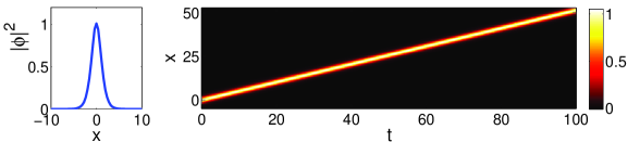
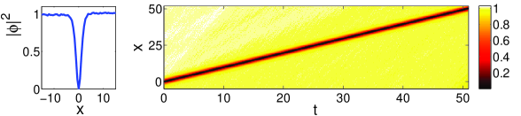
Figure 1. Top panel: The initial density $|\phi|(x,0)|^{2}$ (left panel) of a bright soliton [cf. Eq. (3.24)], and a contour plot showing its evolution under a random small-amplitude perturbation. Parameters: $A=B=1$, $\omega_{0}=-0.5$, $\upsilon=0.5$, $s=1$. Bottom panel: Same as the top panel, but for a dark soliton [cf. Eq. (3.25)] with parameters: $A=B=-1$, $\omega_{0}=1$, $\upsilon=1$, $s=-1$.

The top left panel of Fig. 1 presents the density profile $|\phi|^{2}$ of the initial condition

(3.24) $$\phi_{0}(x)=\mathrm{sech}(0.5x)+\epsilon\cdot\mathrm{noise},\;\;\epsilon=10^{-3},$$

which describes a bright soliton perturbed by a small-amplitude noise. The top right panel of Fig. 1 is a contour plot showing the evolution of the density of the above state. The unperturbed initial bright soliton $u_{bs}(x)=\mathrm{sech}(0.5x)$ has the form of (3.17), for the following choice of parameters suggested from (3.21)-(3.23): $A=B=1$, and $\mu=1$. For this choice of $\mu$, the definition in (3.15) implies that $s=1$. We have also chosen $\omega_{0}=-0.5$, and since $k_{0}=0$, it turns out from (3.14) that $\lambda=0.5$.

The result shown in the top panel of Fig. 1 confirms the existence of the solitary pulse which should be traveling with speed $\upsilon=0.5$ (as it is expected from (3.21)); this is confirmed by the simulation. Additionally, we find that the solitary pulse is robust under this small-amplitude random perturbation; in fact, we have found that the solitary wave persists even for noise amplitudes up to $\epsilon=0.1$.

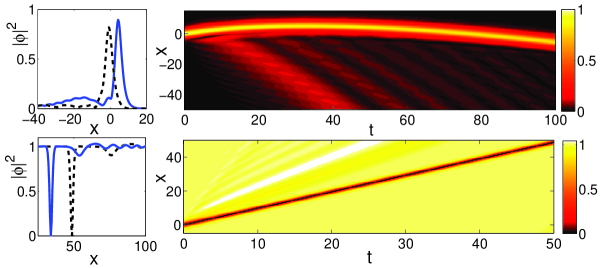
Figure 2. Top panel: Contour plot (right panel) showing the evolution of a bright solitary wave corresponding to the initial condition given in Eq. (3.24) with $\epsilon=0$, for $A/B=0.76$. The bright pulse is accompanied by a small-amplitude radiation as depicted by both the solid (blue)- and the dashed (black) line in the left panel, showing the soliton profile at $t=20$ and $t=60$ respectively. Bottom panel: same as top panel, but for a dark solitary wave, with the initial condition given by Eq. (3.25) with $\epsilon=0$, for $A=-1$, $B=-0.8$, $s=-1$. The left panel shows the density profile at time $t=35$ [dashed (black) curve] and at $t=50$ [solid (blue) curve]. The radiative part emerging on top of the background moves faster than the solitary wave so that, eventually, the solitary wave is separated from the radiation.

We have also studied the case of a dark soliton; corresponding numerical results are presented in the bottom panels of Fig. 1. As before, the initial condition is taken to be a dark soliton perturbed by a small-amplitude uniformly-distributed noise, namely:

(3.25) $$\phi_{0}(x)=\mathrm{tanh}(0.5x)+\epsilon\cdot\mathrm{noise},\;\;\epsilon=10^{-3}.$$

The density of the initial condition (3.25) is shown in the bottom left panel of Fig. 1. The unperturbed initial dark soliton $u_{ds}(x)=\mathrm{tanh}(0.5x)$ is taken from Eq. (3.19), for the following choice of parameters suggested from (3.21)-(3.23): $A=B=-1$ and $\mu=-1$. For this choice of $\mu$, (3.15) implies that $s=-1$. We have also chosen $\omega_{0}=1$, and since $k_{0}=0$, it turns out from (3.14) that $\lambda=1$. The time evolution of the density corresponding to the initial data (3.25) is shown in the contour-plot of the bottom right panel of Fig. 1. As in the previous (bright soliton) case, the existence of the dark solitary pulse travelling with speed $\upsilon=1$ is confirmed [as predicted by (3.21)]; furthermore, the solitary wave is found to be robust under the random perturbation.

Next, we consider the case where the condition for the existence of traveling pulses is violated, i.e., $A\neq B$. Examples corresponding to such a case are shown in Fig. 2, for bright (top panels) and dark (bottom panels) solitons. In particular, the top right panel of Fig. 2 presents the evolution of the density of a bright soliton with the initial form $u_{bs}(x)=\mathrm{sech}(0.5x)$ [corresponding to (3.24) with $\epsilon=0$], with parameter values $A=1$ and $B=1.3$ (i.e. $A/B=0.76$). It is observed that the bright soliton is a traveling one, and emits radiation during its evolution; the radiation is stronger at early times and becomes smaller for later times, tending to disperse away from the pulse; this is depicted in the top left panel, where the soliton profile is shown for $t=20$ (solid line) and $t=60$ (dashed line). Such a behavior has also been observed in the numerical results of [31], and analyzed in [57, 69]. As seen in the contour plot, the soliton initially starts moving towards the positive $x$-direction, but eventually travels with an almost constant velocity towards the negative $x$-direction.

The emission of radiation by the soliton, is also observed in the case of a dark solitary wave, as shown in the bottom panels of Fig. 2; nevertheless, notable differences can be identified in comparison with the bright soliton dynamics, as is explained below. . The left panel of Fig. 2 shows snapshots of the density at two different time instants ($t=35$ and $t=50$), while the initial form of the solitary wave is $u_{ds}(x)=\mathrm{tanh}(0.5x)$ (with $A=-1$, $B=-0.8$, $s=-1$); on the other hand, the right panel shows the evolution of the density. A significant difference with the bright solitary wave is the absence of the turning effect observed in the propagation of the bright soliton: the dark pulse is moving continuously to the positive $x$-direction. As a relevant aside, we also note that ahead of the dark soliton we observe the traces of an apparent dispersive shock wave [34], while in the case of the bright soliton, the relevant radiative wavepackets can only be observed behind the solitary wave. It is also observed that, contrary to the bright solitary wave case, the initial condition tends to a single dark solitary wave moving with an almost constant velocity and a separate radiative part. The latter, travels on top of the continuous-wave background and moves with a velocity larger than that of the dark pulse (the radiative small-amplitude waves in this case travel with the speed of sound), so they eventually separate from each other. Another notable feature is that radiation is emitted in the rear (front) of the bright (dark) solitary wave, due to the different sign of the third-order dispersion parameter $B$: it is positive (negative) for the bright (dark) pulse and, thus, the emission of radiation is directional.

4. Modulation instability

In this section, we will investigate conditions for the modulation instability (MI) of plane-wave solutions of Eq. (3.12) of the form

(4.1) $$\phi^{(0)}(x,t)=\phi_{0}\mathrm{e}^{\mathrm{i}(kx-\omega t)}.$$

Here, the plane wave is assumed to have a constant amplitude $\phi_{0}\in\mathbb{R}$, a wavenumber $k$ and frequency $\omega$. We will show that for $k\neq 0$ there exist essential differences on the MI conditions between the ENLS equation (3.12) and its NLS limit $A=B=0$.

We start by substituting the solution (4.1) into (3.12). We thus obtain the following dispersion relation $\omega(k;\phi_{0}^{2})$:

(4.2) $$\omega=-s\phi_{0}^{2}+3Ask\phi_{0}^{2}+k^{2}-Bk^{3}.$$

We now consider a perturbation of the solution (4.1) of the form:

(4.3) $$\phi(x,t)=\phi^{(0)}(x,t)+\phi^{(1)}(x,t),\;\;\phi^{(1)}(x,t)\in\mathbb{C},\;\;\mbox{for all $x\in\mathbb{R},\;t\in\mathbb{R}$},$$

where $\phi^{(1)}(x,t)$ is assumed to be small in the sense

(4.4) $$|\phi^{(1)}(x,t)|<<|\phi^{(0)}|,\;\;\;\;\mbox{for all $x\in\mathbb{R},\;t\in\mathbb{R}$},$$

while $\phi^{(1)}(x,t)$ is taken to be of the form:

(4.5) $$\phi^{(1)}(x,t)=\mathrm{e}^{\mathrm{i}(kx-\omega t)}\phi_{1}(x,t).$$

Then, $\phi_{1}$ can be decomposed in its real and imaginary parts as:

(4.6) $$\phi_{1}(x,t)=U(x,t)+\mathrm{i}W(x,t),$$

and $U$ and $W$ are considered to be harmonic, i.e.,

(4.7) $$\left(\begin{array}[]{cc}U\\ W\\ \end{array}\right)=\left(\begin{array}[]{c}U_{0}\\ W_{0}\\ \end{array}\right)\mathrm{e}^{\mathrm{i}(Kx-\Omega t)}+c.\;c.\;,\;\;U_{0},\;W_{0}\in\mathbb{R},$$

where $K$ and $\Omega$ are the wave number and frequency of the perturbation, respectively.

Theorem 4.1.

We consider the equation (3.12) with $A,B\in\mathbb{R}$. The plane-wave solutions (4.1) are modulationally unstable (i.e., the perturbations $\phi_{1}(x,t)$ defined by (4.5), (4.6), and (4.7) are growing at exponential rate), if and only if

(4.8) $$1\neq 3Bk,\;\;\mbox{and}\;\;K^{2}<2s\phi_{0}^{2}\left(\frac{1-3kA}{1-3kB}\right).$$

Proof.

Substituting the perturbed solution (4.3) in equation (3.12), linearising as per the smallness condition (4.4), and using the dispersion relation (4.2), we obtain the following equation for $\phi_{1}(x,t)$:

(4.9) $$\phi_{1t} + 3As\phi_{0}^{2}[\phi_{1x}+\mathrm{ik}(\phi_{1}+\bar{\phi}_{1})]-\mathrm{i}(1-3kB)\phi_{1xx}$$

$$+ (2k-3Bk^{2})\phi_{1x}+B\phi_{1xxx}-\mathrm{i}s\phi_{0}^{2}(\phi_{1}+\bar{\phi}_{1})=0.$$

Inserting (4.6) into (4.9), we derive the following equations for $U$ and $W$,

(4.10) $$U_{t}+3As\phi_{0}^{2}U_{x}+(1-3kB)W_{xx}+(2k-3Bk^{2})U_{x}+BU_{xxx}=0,$$

(4.11) $$W_{t}+3As\phi_{0}^{2}(W_{x}+2kU)-(1-3kB)U_{xx}+(2k-3Bk^{2})W_{x}+BW_{xxx}-2s\phi_{0}^{2}U=0.$$

Next, substitution of the expression (4.7) for $U$ and $W$ into (4.10)-(4.11) yields the following algebraic system for $U_{0}$ and $W_{0}$,

(4.13) $$\left\{-\mathrm{i}\Omega+\left[3As\phi_{0}^{2}+k(2-3Bk)\right]\mathrm{i}K-\mathrm{i}BK^{3}\right\}U_{0}-(1-3KB)K^{2}W_{0}=0,$$

$$\left[2s\phi_{0}^{2}(3Ak-1)+(1-3kB)K^{2}\right]U_{0}+\left\{-\mathrm{i}\Omega+\left[3As\phi_{0}^{2}+k(2-3Bk)\right]\mathrm{i}K-\mathrm{i}BK^{3}\right\}W_{0}=0.$$

Seeking for nontrivial solutions $U_{0}$ and $W_{0}$ of the system (4.13)-(4.13), we require the relevant determinant to be zero; this way, we obtain the following dispersion relation:

$$\left\{\Omega-\left[3As\phi_{0}^{2}+k(2-3Bk)\right]K+BK^{3}\right\}^{2}$$

(4.14) $$=K^{2}\left[(1-3kB)^{2}K^{2}-2s\phi_{0}^{2}(1-3Ak)(1-3kB)\right].$$

From (4) the MI condition for plane waves (4.1) readily follows. For instance, assuming that $1\neq 3kB$, it is required that

(4.15) $$(1-3kB)^{2}K^{2}<2s\phi_{0}^{2}(1-3Ak)(1-3kB),$$

or equivalently, (4.8). ∎

It is relevant to consider certain limiting cases of (4). First, if $k=0$ (i.e., the plane wave is stationary), Eq. (4) is reduced to the form:

(4.16) $$(\Omega-3AKs\phi_{0}^{2}+BK^{3})^{2}=K^{2}(K^{2}-2s\phi_{0}^{2}).$$

The above equation has two solutions

(4.17) $$\Omega=3AKs\phi_{0}^{2}-BK^{3}\pm K\sqrt{K^{2}-2s\phi_{0}^{2}}.$$

The frequency $\Omega$ becomes complex (i.e., $\Omega=\Omega_{\rm r}+i\Omega_{\rm i}$) if and only if

(4.18) $$s=1,\qquad K^{2}-2\phi_{0}^{2}<0.$$

The above are the same as the conditions for MI of plane wave solutions of the NLS equation ($A=B=0$); note that in the case $s=-1$, (4.17) implies that the plane wave is always modulationally stable, as in the (defocusing) NLS case. Thus, for $k=0$, the only difference from the NLS limit is that in the ENLS case there exists a nonvanishing real (oscillatory) part of the perturbation frequency, i.e., $\Omega_{\mathrm{r}}=3AKs\phi_{0}^{2}-BK^{3}$, as suggested by (4.17). Additionally, it is observed that in the NLS limit $A=B=0$, the well-known result (see, e.g., [4, 32]) that the MI condition for the focusing NLS model ($s=1$) does not depend on $k$ is recovered.

On the other hand, in the framework of the ENLS with $A,B\neq 0$, and $k\neq 0$, condition (4.8) reveals some important differences between the ENLS equation with its NLS limit. First, the instability criterion is modified for the focusing case ($s=+1$), as seen by a direct comparison of (4.8) and (4.18). Secondly, and even more importantly, condition (4.8) shows that plane waves (4.1) can be modulationally unstable also in the defocusing ($s=-1$) case, contrary to what happens in the defocusing NLS limit where such an instability is absent. Thus concluding, for the ENLS model, continuous waves with $k=0$ can be modulationally unstable only in the focusing case $s=1$, while plane waves of the form of equation (4.1) with $k\neq 0$, can be modulationally unstable in both the focusing $s=1$ and the defocusing case $s=-1$ (for an appropriate choice of parameters).

Let us now define the instability band, as the closed interval $B_{I}=[K_{\mathrm{min}},K_{\mathrm{max}}]$ (for fixed $\phi_{0}$) for the wavenumbers of the perturbations of (4.5) with the following property: For every $K\in B_{I}$, the condition (4.8) is satisfied, and the solutions of the quadratic equation (4) in terms of $\Omega$ are complex conjugates. The imaginary parts of these solutions are responsible for the exponential growth of the perturbations (4.5), implying the MI of the plane wave (4.1). In particular, $\mathrm{Im}(\Omega)=\Omega_{i}$ can be plotted as a function of $K\in B_{I}$. The possible maximum of this curve, denoted by $\Omega_{\mathrm{crit}}$, attained on $K_{\mathrm{crit}}\in B_{I}$ is associated with the maximum growth of the unstable perturbations.

We conclude the discussion on the MI effects of the solutions (4.1) with $k\neq 0$, by explicitly showing, that a choice of a wave number $K=K_{0}\in B_{I}$ for the perturbations (4.5), implies the excitation of the integer multiples of $K_{0}$ for the unstable wave solutions, i.e., the wave numbers of the unstable plane wave solutions are $k\pm nK_{0}$, $n\in\mathbb{N}$. To show this, we start by rewriting the perturbed plane wave (4.17) accounting the complex conjugates (c.c.) of the perturbations (4.5), i.e.,

(4.19) $$\phi(x,t)=\left[\phi_{0}+U_{0}\mathrm{e}^{\mathrm{i}(Kx-\Omega t)}+c.c.+\mathrm{i}(W_{0}\mathrm{e}^{\mathrm{i}(Kx-\Omega t)}+c.c)\right]\mathrm{e}^{\mathrm{i}\theta},\;\;\theta=kx-\omega t.$$

We consider the unstable wave number $K_{0}\in B_{I}$ and the associated imaginary part $\Omega_{i}=\Omega_{i}(K_{0})$. Then, (4.19) may be written as $\phi(x,t)=R\mathrm{e}^{\mathrm{i}\varphi}\mathrm{e}^{\mathrm{i}\theta}$, where $R$ and $\varphi$ are respectively given by:

(4.20) $$R = \left[\phi_{0}^{2}+4\phi_{0}U_{0}\mathrm{e}^{\Omega_{i}t}+4(U_{0}^{2}+W_{0}^{2})\mathrm{e}^{2\Omega_{i}t}\cos^{2}(K_{0}x)\right]^{\frac{1}{2}},$$

(4.21) $$\varphi=\arctan\left[\frac{2W_{0}\mathrm{e}^{\Omega_{i}t}\cos(K_{0}x)}{\phi_{0}+2U_{0}\mathrm{e}^{\Omega_{i}t}\cos(K_{0}x)}\right].$$

Note that since $U_{0},W_{0}\ll 1$, equations (4.20) and (4.21) can be approximated as:

(4.22) $$R\approx\phi_{0}\left[1+\frac{2U_{0}}{\phi_{0}}\mathrm{e}^{\Omega_{i}t}\cos(K_{0}x)\right],$$

and

(4.23) $$\varphi\approx\frac{2W_{0}}{\phi_{0}}\mathrm{e}^{\Omega_{i}t}\cos(K_{0}x).$$

Then, using (4.22) and (4.23), the perturbed plane wave (4.19) can be written as

(4.24) $$\phi(x,t)\approx\phi_{0}\left[1+\frac{2U_{0}}{\phi_{0}}\mathrm{e}^{\Omega_{i}t}\cos(K_{0}x)\right]\mathrm{e}^{\mathrm{i}\mathcal{R}\sin\chi}\mathrm{e}^{\mathrm{i}\theta},$$

where $\mathcal{R}=\frac{2W_{0}}{\phi_{0}}\mathrm{e}^{\Omega_{i}t}$ and $\chi=\frac{\pi}{2}-K_{0}x$. However, using the formula (see [2, 30]),

$$\mathrm{e}^{\mathrm{i}\mathcal{R}\sin\chi}=\sum_{n=-\infty}^{+\infty}J_{n}(\mathcal{R})\mathrm{e}^{\mathrm{i}n\chi},$$

where $J_{n}$ denotes the Bessel function of the first kind of integer order $n$, we find that (4.24) eventually is approximated as

(4.25) $$\phi(x,t)\approx\phi_{0}\left[1+\frac{2U_{0}}{\phi_{0}}\mathrm{e}^{\Omega_{i}t}\cos(K_{0}x)\right]\sum_{n=-\infty}^{+\infty}J_{n}(\mathcal{R})\mathrm{e}^{\mathrm{i}(\theta+n\chi)},$$

where

(4.26) $$\mathrm{e}^{\mathrm{i}(\theta+n\chi)}=\exp\left\{\mathrm{i}\left[kx-\omega t+n\left(\frac{\pi}{2}-K_{0}x\right)\right]\right\}.$$

It is evident from the expression of the solution (4.25)-(4.26) that the wave numbers of the unstable plane wave solution are $k\pm nK_{0}$, $n\in\mathbb{Z}$, when the choice $K_{0}\in B_{I}$ is made. Notice that the above calculation is valid even in the case where $\Omega_{i}=0$, however in the latter case the wavenumbers $k\pm nK_{0}$ are not subject to growth.

4.1. Numerical study 2: Modulation instability of plane waves

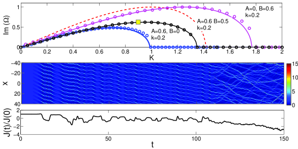
Figure 3. Top panel: The growth rate $\mathrm{Im}(\Omega)=\Omega_{i}$ as a function of the wavenumber $K$ of the perturbation, and the associated instability bands $B_{I}=[0,K_{\mathrm{max}}]$, for the ENLS equation (3.12) with $s=+1$. The solid lines and circles correspond, respectively, to the analytical and numerical results, while the dotted (red) line corresponds to the focusing NLS limit with $A=B=0$. Other parameter values are: $k=0.2$, $\phi_{0}=1$. Middle panel: Contour plot showing the evolution of the density $|\phi|^{2}$ as found numerically for $A=0.6,B=0.5$, and initial data as per (4.27) with $k=0.2$, $\epsilon=2U_{0}=10^{-3}$ and $K=0.9$ (i.e., pertaining to the square of the top panel). Bottom panel: Evolution of the normalized functional $\mathbf{J}(t)/\mathbf{J}(0)$.

In this section, we numerically integrate equation (3.12), using as an initial condition the perturbed plane-wave:

(4.27) $$\phi(x,0)\approx\phi_{0}\left[1+\frac{2U_{0}}{\phi_{0}}\cos(K_{0}x)\right]\mathrm{e}^{\mathrm{i}kx},$$

with $k\neq 0$ and parameters $\phi_{0}=1$ and $2U_{0}=\epsilon=10^{-3}$. We then calculate the growth rate of the amplitude of the initial plane wave, and compare it with the above analytical results. Figure 3 presents the comparison of numerical computations with the ENLS equation (3.12) and $s=1$, for various values of the parameters $A,B\in\mathbb{R}$ and for fixed $k=0.2$. The upper panel of Fig. 3 shows the analytically computed curves $\mathrm{Im}(\Omega)(K)=\Omega_{i}(K)$, and the relative instability bands $B_{I}=[0,K_{\mathrm{max}}]$ against their numerically computed counterparts. The analytical curves $\Omega_{i}(K)$ are depicted by solid lines, while the respective numerical results are shown by circles. The dotted (red) line corresponds to the analytical result for the focusing NLS-limit ($A=B=0$). The solid lines correspond to the ENLS equation for $A=0,B=0.6$ [upper (magenta) line], $A=0.6,B=0.5$ [middle (black) line] and $A=0.6,B=0$ [lower (blue) line]. In all cases we observe the excellent agreement of the analytical prediction for the growth rates of the plane wave with the numerical results. Another interesting observation is the progressive increase of the length of the MI-bands, from the limit of $A\neq 0$ and $B=0$, i.e., from the NLS equation with the self-steepening effect, to the limit of $A=0,B\neq 0$, i.e., to the NLS equation with the third-order dispersion effect (see, e.g. [4] for a discussion of these effects on the NLS model). It is clear that if $1-3kB>0$ in (3.12), increase of $A$ will have a stabilizing effect, while for $1-3kB<0$, it will have a destabilizing effect. The role of $B$ is, roughly, reversed with respect to that of $A$, although the associated functional dependence is structurally somewhat more complex.

The contour plot in the middle panel of Fig. 3 shows the evolution of the density $|\phi|^{2}$ for a case where both $A$ and $B$ are nonzero, namely for $A=0.6,B=0.5$; here, the wavenumbers of the plane wave and of the perturbation are chosen as $k=0.2$ and $K=0.9$, respectively. The growth rate for this case, $\Omega_{i}(0.9)$, is marked with the (yellow) square in the top panel of Fig. 3, in the relevant curve. The contour plot illustrates the manifestation of the MI and the concomitant dynamics. In particular, at the initial stage of the evolution, one can observe the formation of an almost periodic pattern characterized by the excitation of the unstable wavenumber $K=K_{0}=0.9$, and at a later stage (for $t\gtrsim 120$) the formation of traveling localized structures induced by the manifestation of MI.

It is also interesting to make the following observation. In the bottom panel of Fig. 3, we show the evolution of the normalized functional $\mathbf{J}(t)/\mathbf{J}(0)$, for the parameter values used in the middle panel of the same figure (recall that $A\neq B$ in this case), i.e., in the case where MI manifests itself. It is observed that, prior to the onset of MI, the above functional assumes a constant value which, however, changes upon the onset of MI. In particular, as seen in this panel, the initial value $\mathbf{J}(0)$ is preserved until the appearance of the first pattern of localized structures: at that instance, $\mathbf{J}$ first decreases and, for later times, fluctuates. This effect can be explained by the equation

(4.28) $$\frac{d}{dt}\mathbf{J}(\phi(t)+\frac{3}{2}\mathrm{Re}\left[\int_{\Omega}(|\phi|^{2})_{x}|\phi_{x}|^{2}dx\right](\delta\sigma-\alpha\rho)=0.$$

derived in the proof of Lemma 2.3 and (2.26). If plane waves of the form of Eq. (4.1) are modulationally stable, then $|\phi|^{2}\sim\phi_{0}^{2}$ and $|\phi|_{x}^{2}\sim 0$, for all times. Therefore, (4.28) implies that when $A\neq B$, this quantity should be (roughly) conserved and, thus, $\frac{d}{dt}\mathbf{J}(\phi(t)=0$ in the modulationally stable regime. On the other hand, in the modulationally unstable regime, there exists a time $T_{\mathrm{MI}}$, such that the perturbation $\phi_{1}(x,t)$ should become significant for all $t\geq T_{\mathrm{MI}}$. Therefore, in the case $A\neq B$ and in the MI regime, $\mathbf{J}$ cannot be (nearly) conserved for all times, and $\frac{d}{dt}\mathbf{J}(\phi(t)\neq 0$, for all $t\geq T_{\mathrm{MI}}$. Thus, in this set of cases the NLS-based (energy) functional $\mathbf{J}(t)$ may be used as a diagnostic of MI for the nonintegrable case of $A\neq B$. However, this effect is not apparent in the integrable case of $A=B$, where $\mathbf{J}$ is always conserved, by virtue of Eq. (4.28) and for this reason, the non-conservation of the Hamiltonian energy $\mathbf{J}(t)$ cannot be used as a generic diagnostic tool for the detection of MI. In the latter case of $A=B$ (as well as for $A\neq B$), other tools can be used to detect the instability, such as, e.g., the functional $\tilde{{\bf J}}(t)=\int\phi(x,t)\phi^{\star}(x+a,t)dx$ (for an arbitrary fixed $a$), by analogy to the quantity $\sum_{j}\phi_{j}(t)\phi_{j+1}^{\star}(t)$ used for discrete NLS models. Here, for the latter case of $A=B$, we will resort to Fourier space diagnostics that will also clearly allow us to detect the relevant instability.

Next, in Fig. 4 we present numerical results for the ENLS equation (3.12) with $s=-1$ (i.e., in defocusing settings). The solid lines (circles) correspond to the analytical (numerical) results for three different cases: (i) $A=0,B=0.6$, $k=0.72$, characterized by the “large” instability band $B_{I}$ (magenta); (ii) $A=1,B=0.5$, $k=0.5$, with the “medium” instability band (black); (iii) $A=0.6,B=0$, $k=1$, with the “small” instability band (black). Once again, we observe the excellent agreement between analytical and numerical results for the growth rates. Notice that, in this figure, instability band for the defocusing NLS-limit does not exist since plane waves are modulationally stable in this limit. The broadening of the instability band from the limits corresponding to the NLS with the self-steepening term ($A=0$, $B\neq 0$) to the NLS with the third-order dispersion term ($A\neq 0$, $B=0$) observed in Fig. 4, can also be observed in this case.

In the bottom panel of Fig. 4, we show the space-time evolution of the density $|\phi|^{2}$, and the manifestation of the MI, for the more general case of $A,B\neq 0$, i.e., for parameter values $A=1,B=0.5$, as well as for $k=0.5$ and for an unstable wavenumber $K=K_{0}=1$. The perturbation growth $\Omega_{i}(1)$ is marked with the (green) square in the top panel of the same figure in the respective $\Omega_{i}(K)$ curve. The initial stage of the dynamics is qualitatively similar to that in the middle panel of Fig. 3, but the later stage (for times $t\gtrsim 120$) is not characterized by the emergence of travelling localized structures: in the specific parameter regime, we have checked (results not shown here) that such structures are not supported by the system, contrary to the case of Fig. 3 where such states do exist.

For completeness, in Fig. 5 we show the Fourier transform $|\Phi(k)|$, of a modulationally unstable solution, corresponding to the ENLS equation in the focusing nonlinearity case of $s=1$, with parameters $A=B=0.6$, $k=0.2$ and $K_{0}=0.9$; shown is the Fourier spectrum at a time instant after the instability has set in. The figure clearly demonstrates the fact that once MI manifests itself, wave numbers $k\pm nK_{0}$, $n\in\mathbb{N}$ are generated, as was illustrated above.

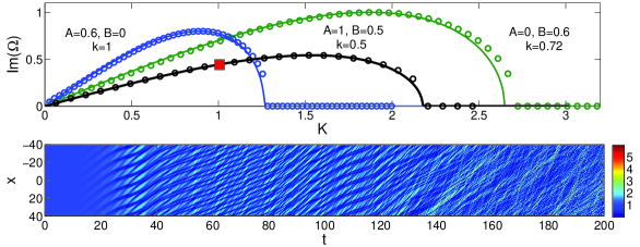
Figure 4. Top and bottom panels are same as corresponding ones in Fig. 3, but for the case of defocusing nonlinearity $s=-1$, and for $A=1,B=0.5$, $k=0.5$, $\epsilon=2U_{0}=10^{-3}$ and $K=1$.

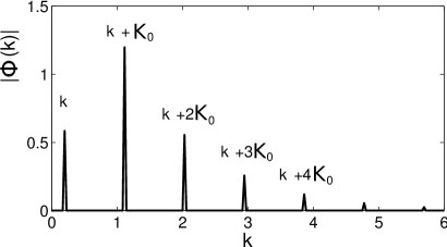
Figure 5. Fourier spectrum $\Phi(k,t=50)$ of the unstable plane wave solution in the focusing case $s=1$, for parameters $A=B=0.6$, and perturbed plane wave initial data (4.27) with $\phi_{0}=1$, $k=0.2$, $\epsilon=2U_{0}=10^{-3}$ and $K_{0}=0.9$; one can observe the excitation of the wave numbers $k+nK_{0}$.

5. Discussion and conclusions

In this work, analytical studies corroborated by numerical simulations, considered various aspects of the solutions of the ENLS equation (1.1) which, under the balance condition (1.2), corresponds to the integrable Hirota equation. The ENLS equation is an important model finding applications in various mathematical and physical settings; these include geometric evolution equations, the evolution of vortex filaments (in the integrable focusing case), and propagation of short pulses in nonlinear optical fibers and nonlinear metamaterials.

Firstly, the global existence of $H^{2}$-weak solutions for the periodic initial-boundary value problem has been established. The global well-posedness in this regularity class, was an application of the justification of an $H^{2}$-type “energy equation” and the conservation laws satisfied by the weak solutions. Such questions are of importance, since the model may fall in the class of dispersive equations with lower-order non-linearities, but for which the periodic initial-boundary value problem may, in principle, exhibit finite time singularities. It was shown that the balance condition on the coefficients, and the assumption of non-vanishing second-order dispersion, are sufficient to guarantee the global-in-time solvability for the prescribed class of initial data.

Next, we investigated the existence of exact travelling wave solutions, and focused –in particular– on the existence of dark and bright solitary waves. The reduction of the problem to an ODE in the traveling wave frame revealed that the balance condition (1.2) is essential; in fact, it was found that it coincides with the compatibility assumptions needed to be satisfied by the system of ODE’s governing the envelope of the desired travelling wave solution. The consideration of the reduced 2nd-order conservative dynamical system for the envelope, led to parameter regimes (including the frequency and the wavenumber of the travelling wave) for the existence of bright and dark solitary wave solutions; these soliton solutions are respectively given by:

$$\phi(x,t) = \pm\sqrt{2\lambda}\,\mathrm{sech}\left[\sqrt{\lambda}\,(x-\upsilon t)\right]\mathrm{e}^{\mathrm{i}(k_{0}x-\omega_{0}t)},\;\;\lambda>0,$$

$$\phi(x,t) = \pm\sqrt{|\lambda|}\mathrm{tanh}\left[\sqrt{\frac{|\lambda|}{2}}(x-\upsilon t)\right]\mathrm{e}^{\mathrm{i}(k_{0}x-\omega_{0}t)},\;\;\lambda<0,$$

(cf. definitions and conditions on parameters $\lambda,\omega_{0},k_{0},\upsilon$ in Section 3). Importantly, we found that standing wave solutions, corresponding to $k_{0}=v=0$, do not exist –contrary to the case of the NLS model. Additionally, it was interesting to find that, apart from the balance condition, new conditions on dispersion and nonlinearity coefficients should be satisfied in order for the above travelling solitons to exist. For instance, we found that solitons may also exist at the zero dispersion point (where 2nd-order dispersion vanishes), in which case the ENLS is reduced to the cmKdV equation.

We have also presented results of direct numerical simulations of the ENLS equation, with initial data corresponding to randomly perturbed bright and dark solitons. Our results, corresponding to the integrable limit, indicate that the analytically determined soliton solutions are robust under perturbations. On the other hand, numerical results corresponding to the case where the balance condition is not satisfied, have shown that bright and dark soliton initial conditions evolve to corresponding localized pulses that continuously emit radiation. Some of the results – and particularly those corresponding to bright solitons – were found to be in accordance with the findings of Refs. [31, 57, 69]. Nevertheless, important differences were identified between the evolution of bright and dark pulses, concerning the radiation emission dynamics and the direction of their propagation.

Finally, we carried out a detailed analysis of the modulation instability (MI) of the plane wave solutions of the ENLS, namely,

$$\phi(x,t)=\phi_{0}\mathrm{e}^{\mathrm{i}(kx-\omega t)},$$

and identified crucial differences between the ENLS equation and the corresponding NLS limit. For travelling plane waves, with wave number $k\neq 0$, it was shown that modulation instability can occur for both the focusing ($s=+1$) and the defocusing ($s=-1$) ENLS equation. The latter result is in contrast with the defocusing NLS limit, where such plane waves are always modulationally stable. In the case of stationary plane waves, with wave number $k=0$, the focusing ENLS equation possesses the same properties with its NLS counterpart, in the sense that MI conditions (and, as a result, the instability bands) coincide. Also, interesting properties were revealed concerning the dependence of the instability bands on the higher-order effects. These properties refer to the NLS equation with the self-steepening effect (corresponding to the case $A=0,B\neq 0$ of the ENLS (3.12)) and the NLS equation with the 3rd-order dispersion (corresponding to the case $A\neq 0,B=0$ of the ENLS (3.12)). It was found that the ENLS equation with $A,B\neq 0$ possesses a MI band of intermediate length between the respective MI band of the self-steepening limit (having the smallest MI band), and the 3rd-order dispersion limit (having the largest MI band).

The results presented in this paper may pave the way for future work in many interesting directions. One such direction is to investigate the dynamics of weakly smooth initial data, when the sufficient conditions for global existence are not satisfied; is such a case, it would be relevant to seek for parameteric regimes in which possible instabilities, and even collapse, may emerge. Another direction is to examine the applicability of our results –especially those pertaining to the defocusing case– in the context of general curve evolution problems and geometric evolution equations. One could follow relevant studies on the geometric characterization of the defocusing NLS [18] or for the nonintegrable case [53, 55]. Additionally, regarding the stability of the solutions, it would be interesting to extend the program developed in [13, 46] (for studying the stability of closed solutions of the NLS equation and their correspondence to the vortex filament motion) to the integrable focusing ENLS (Hirota) equation. Such studies are currently in progress and will be presented in future publications.

Appendix A Approximation scheme for the derivation of the energy equations

In this complementary section, we include for the sake of completeness, the details of the proof of Lemma 2.4. For the justification of various computations needed for the derivation of the energy equation, we recall some useful lemmas concerning time differentiation of Hilbert space valued functions [22, 65].

Lemma A.1.

Let $V_{i}\subset H\subset V_{i}^{\prime}$, $i=1,2$ a sequence of real Hilbert spaces, with continuous inclusions. If $\phi_{i}\in L^{2}([0,T],V_{i})$, $\partial_{t}\phi_{1}\in L^{2}([0,T],V_{2}^{\prime})$ and $\partial_{t}\phi_{2}\in L^{2}([0,T],V_{1}^{\prime})$ then

$$\partial_{t}(\phi_{1},\phi_{2})=<\phi_{2},\partial_{t}\phi_{1}>_{{\scriptscriptstyle V_{2},V_{2}^{\prime}}}+<\phi_{1},\partial_{t}\phi_{2}>_{{\scriptscriptstyle V_{1},V_{1}^{\prime}}}.$$

Lemma A.2.

Let $V\subset H\subset V^{\prime}$ be three real Hilbert spaces, with continuous inclusion. We assume that $V$ is a generalized Banach algebra and

$$\begin{gathered}<\phi,\psi>_{{\scriptscriptstyle V,V^{\prime}}}=(\phi,\psi)_{\scriptscriptstyle H},\quad\forall\,\phi\in V,\quad\forall\,\psi\in H,\\ <\phi,z\,\psi>_{{\scriptscriptstyle V,V^{\prime}}}=<\phi\,\psi,z>_{{\scriptscriptstyle V,V^{\prime}}},\quad\forall\,\phi,\psi\in V,\quad\forall\,z\in V^{\prime}.\end{gathered}$$

Moreover, we assume that $\psi_{i}\in L^{2}([0,T],V)$ and $\partial_{t}\psi_{i}\in L^{2}([0,T],V^{\prime})$ for $i=1,2$. Then the (weak) derivative $\partial_{t}(\psi_{1}\psi_{2})$ exists and

$$<\phi,\partial_{t}(\psi_{1}\psi_{2})>_{{\scriptscriptstyle V,V^{\prime}}}=<\phi,\partial_{t}\psi_{1}\,\psi_{2}+\psi_{1}\,\partial_{t}\psi_{2}>_{{\scriptscriptstyle V,V^{\prime}}},\quad\forall\,\phi\in V.$$

Now, let us consider the unique solution $\phi\in C([0,T],H^{3}_{per}(\Omega))\cap C^{1}([0,T],L^{2}(\Omega))$ of (1.1)-(2.2)-(2.1). From Lemmas A.1 and A.2, it follows that (see also [65, Proposition 2.1, p. 170, eq. (2.17)])

(A.1) $$\begin{gathered}\phi_{txx}\in L^{2}([0,T],H^{-2}_{per}(\Omega)),\quad\phi_{tx}\in L^{2}([0,T],H^{-1}_{per}(\Omega)),\\ \phi_{xxxx}\in L^{2}([0,T],H^{-1}_{per}(\Omega)),\\ \phi_{txx}=\phi_{xtx}=\phi_{xxt},\quad\phi_{tx}=\phi_{xt}.\end{gathered}$$

Accordingly, the infinitely smooth approximating function $v_{n}$ converges to the solution $\phi$ in the spaces

(A.2) $$\begin{array}[]{lllll}v_{n}\rightharpoonup\phi,\;\;\mbox{in}\;\;L^{2}([0,T],H^{3}_{per}(\Omega)),&&\;v_{nx}\rightharpoonup\phi_{x},\;\;\mbox{in}\;\;L^{2}([0,T],H^{2}_{per}(\Omega)),\\ v_{nt}\rightharpoonup\phi_{t},\;\;\mbox{in}\;\;L^{2}([0,T],L^{2}(\Omega)),&&\;v_{nxx}\rightharpoonup\phi_{xx},\mbox{in}\;\;L^{2}([0,T],H^{1}_{per}(\Omega)),\\ v_{ntx}\rightharpoonup\phi_{tx},\;\;\mbox{in}\;\;L^{2}([0,T],H^{-1}_{per}(\Omega)),&&\;v_{nxxx}\rightharpoonup\phi_{xxx},\mbox{in}\;\;L^{2}([0,T],L^{2}(\Omega)),\\ v_{ntxx}\rightharpoonup\phi_{txx},\;\;\mbox{in}\;\;L^{2}([0,T],H^{-2}_{per}(\Omega)),&&\;v_{nxxxx}\rightharpoonup\phi_{xxxx},\mbox{in}\;\;L^{2}([0,T],H^{-1}_{per}(\Omega)),\end{array}$$

as a consequence of Theorem 2.1. Now, we proceed to approximate the time derivative of the second term of of the functional (2.27) as follows:

(A.3) $$\begin{split}\tfrac{d}{dt}\left(|v_{nx}|^{2},|v_{n}|^{2}\right)_{\scriptscriptstyle L^{2}}=&\,\left<|v_{n}|^{2},\tfrac{d}{dt}|v_{nx}|^{2}\right>_{\scriptscriptstyle H^{2},H^{-2}}+\left<|v_{nx}|^{2},\tfrac{d}{dt}|v_{n}|^{2}\right>_{\scriptscriptstyle H^{2},H^{-2}}\\ =&\,2\,\left<|v_{n}|^{2},\overline{v}_{nx}v_{nxt}\right>_{\scriptscriptstyle H^{2},H^{-2}}+2\,\left<|v_{nx}|^{2},\overline{v}_{n}v_{nt}\right>_{\scriptscriptstyle H^{2},H^{-2}}\\ =&\,2\,\left<|v_{n}|^{2}\overline{v}_{nx},v_{nxt}\right>_{\scriptscriptstyle H^{2},H^{-2}}+\left<|v_{nx}|^{2}\overline{v}_{n},v_{nt}\right>_{\scriptscriptstyle H^{2},H^{-2}}\\ =&\,-2\,\left<|v_{n}|^{2}\overline{v}_{nxx},v_{nt}\right>_{\scriptscriptstyle H^{1},H^{-1}}-2\left<\overline{v}^{2}_{nx}v_{n},v_{nt}\right>_{\scriptscriptstyle H^{2},H^{-2}}\\ &\quad-2\left<|v_{nx}|^{2}\overline{v}_{n},v_{nt}\right>_{H^{2},H^{-2}}+2\left<|v_{nx}|^{2}\overline{v}_{n},v_{nt}\right>_{\scriptscriptstyle H^{2},H^{-2}}\\ =&\,-2\,\left<|v_{n}|^{2}\overline{v}_{nxx},v_{nt}\right>_{\scriptscriptstyle H^{1},H^{-1}}-2\left<\overline{v}_{nx}^{2}v_{n},v_{nt}\right>_{\scriptscriptstyle H^{2},H^{-2}}.\\ \end{split}$$

Integration of (A.3) with respect to time, gives (2.33), from which we are passing to the limit equation (2.35), as discussed in the Lemma 2.4. Proceeding further, the substitution of $\phi_{t}$ into (2.35), in terms of its expression given by the pde (2.16), can be handled with the computations

(A.4) $$\begin{split}-2\left<|\phi|^{2}\,\overline{\phi}_{xx},\phi_{t}\right>_{\scriptscriptstyle H^{1},H^{-1}}=&\,-2\,\left<|\phi|^{2}\,\overline{\phi}_{xx},-3\,\alpha\,|\phi|^{2}\,\phi_{x}+{\rm i}\,\rho\,\phi_{xx}-\sigma\,\phi_{xxx}+{\rm i}\,\delta\,|\phi|^{2}\,\phi\right>_{\scriptscriptstyle H^{1},H^{-1}}\\ =&\,6\,\alpha\,\left<\overline{\phi}_{xx}\,\phi_{x},|\phi|^{4}\right>_{\scriptscriptstyle H^{1},H^{-1}}+2\,\sigma\,\left<|\phi|^{2}\,\overline{\phi}_{xx},\phi_{xxx}\right>_{\scriptscriptstyle H^{1},H^{-1}}\\ &\quad-2\,\delta\,\left<\overline{\phi}_{xx},{\rm i}\,|\phi|^{4}\,\phi\right>_{\scriptscriptstyle H^{1},H^{-1}},\\ \left<\overline{\phi}_{x}^{2}\,\phi,\phi_{t}\right>_{\scriptscriptstyle H^{2},H^{-2}}=&\,6\,\alpha\,\left<\overline{\phi}_{x}^{2}\,\phi,|\phi|^{2}\,\phi_{x}\right>_{\scriptscriptstyle H^{2},H^{-2}}-2\rho\left<\overline{\phi}_{x}^{2}\,\phi,\phi_{xx}\right>_{\scriptscriptstyle H^{2},H^{-2}}\\ &\,+2\,\sigma\,\left<\overline{\phi}_{x}^{2}\,\phi,\phi_{xxx}\right>_{\scriptscriptstyle H^{2},H^{-2}}-2\,\delta\,\left<\overline{\phi}_{x}^{2}\,\phi,{\rm i}\,|\phi|^{2}\,\phi\right>_{\scriptscriptstyle H^{2},H^{-2}}.\\ \end{split}$$

Now, by using (2.31), (2.35), and (A.4), we derive the equation

(A.5) $$\begin{split}\tfrac{d}{dt}\int_{\scriptscriptstyle\Omega}|\phi_{x}|^{2}|\phi|^{2}\,dx=&\,3\,\alpha\,\mathrm{Re}\left[\int_{\scriptscriptstyle\Omega}|\phi|^{4}\,(|\phi_{x}|^{2})_{x}\;dx\right]+\sigma\,\mathrm{Re}\left[\int_{\scriptscriptstyle\Omega}|\phi|^{2}\,(|\phi_{xx}|^{2})_{x}\;dx\right]\\ &+2\,\delta\,\mathrm{Im}\left[\int_{\scriptscriptstyle\Omega}|\phi|^{4}\,\phi\,\overline{\phi}_{xx}\;dx\right]+3\,\alpha\,\mathrm{Re}\left[\int_{\scriptscriptstyle\Omega}|\phi|^{2}\,|\phi_{x}|^{2}\,(|\phi|^{2})_{x}\;dx\right]\\ &+2\,\sigma\,\mathrm{Re}\left[\int_{\scriptscriptstyle\Omega}\overline{\phi}_{x}^{2}\,\phi\,\phi_{xxx}\;dx\right]+2\,\rho\,\mathrm{Im}\left[\int_{\scriptscriptstyle\Omega}\overline{\phi}_{x}^{2}\,\phi\,\phi_{xx}\;dx\right]\\ &+2\,\delta\,\mathrm{Im}\left[\int_{\scriptscriptstyle\Omega}\overline{\phi}_{x}^{2}\,\phi^{2}|\phi|^{2}\;dx\right],\\ \end{split}$$

being valid for the solution $C([0,T],H^{3}_{per}(\Omega))\cap C^{1}([0,T],L^{2}(\Omega))$.

We compute next, the time derivatives for the remaining terms of the functional (2.27). For the term $(\phi^{2},\overline{\phi}_{x}^{2})_{\scriptscriptstyle L^{2}(\Omega)}$, by using the approximating sequence $v_{n}$, and Lemmas A.1 and A.2, we observe that

(A.6) $$\begin{split}\tfrac{d}{dt}\left(v_{n}^{2},\overline{v}^{2}_{nx}\right)_{\scriptscriptstyle L^{2}(\Omega)}&=\left<\overline{v}^{2}_{nx},\tfrac{d}{dt}v_{n}^{2}\right>_{\scriptscriptstyle H^{2},H^{-2}}+\left<v_{n}^{2},\tfrac{d}{dt}\overline{v}_{nx}^{2}\right>_{\scriptscriptstyle H^{2},H^{-2}}\\ &=2\,\left<\overline{v}^{2}_{nx}v_{n},v_{nt}\right>_{\scriptscriptstyle H^{2},H^{-2}}+2\,\left<\overline{v}^{2}v_{nx},v_{nxt}\right>_{\scriptscriptstyle H^{2},H^{-2}}\\ &=2\,\left<\overline{v}^{2}_{nx}v_{n},v_{nt}\right>_{\scriptscriptstyle H^{2},H^{-2}}-2\,\left<\partial_{x}(\overline{v}_{n}^{2}v_{nx}),v_{nt}\right>_{\scriptscriptstyle H^{1},H^{-1}}\\ &=2\,\left<\overline{v}^{2}_{nx}v_{n},v_{nt}\right>_{\scriptscriptstyle H^{2},H^{-2}}-4\left<\overline{v}_{n}|v_{nx}|^{2},v_{nt}\right>_{\scriptscriptstyle H^{2},H^{-2}}-2\left<\overline{v}_{n}^{2}v_{nxx},v_{nt}\right>_{\scriptscriptstyle H^{1},H^{-1}}.\\ \end{split}$$

We continue by using the same arguments, as for the derivation of (2.35). Letting $n\rightarrow\infty$ we get that

(A.7) $$\tfrac{d}{dt}(\phi^{2},\overline{\phi}_{x}^{2})_{\scriptscriptstyle L^{2}(\Omega)}=\mathbf{I_{1}}+\mathbf{I_{2}}+\mathbf{I_{3}},$$

where the terms $(\mathbf{I_{k}})_{k=1}^{3}$ are found to be

(A.8) $$\begin{split}\mathbf{I_{1}}=&\,2\,\left<\phi\,\overline{\phi}_{x}^{2},\phi_{t}\right>_{\scriptscriptstyle H^{2},H^{-2}}-3\,\alpha\,\left<|\phi|^{2}\,|\phi_{x}|^{2},\partial_{x}\,(|\phi|^{2})\right>_{\scriptscriptstyle H^{2},H^{-2}}\\ &+2\,\rho\,\left<\phi\,\overline{\phi}_{x}^{2},{\rm i}\,\phi_{xx}\right>_{\scriptscriptstyle H^{2},H^{-2}}-2\,\sigma\,\left<\phi\,\overline{\phi}_{x}^{2},\phi_{xxx}\right>_{\scriptscriptstyle H^{2},H^{-2}}+2\,\delta\,\left<\overline{\phi}_{x}^{2},{\rm i}|\phi|^{2}\,\phi^{2}\right>_{\scriptscriptstyle H^{2},H^{-2}},\\ \end{split}$$

(A.9) $$\begin{split}\mathbf{I_{2}}=&-4\,\left<\overline{\phi}\,|\phi_{x}|^{2},\phi_{t}\right>_{\scriptscriptstyle H^{2},H^{-2}}+6\,\alpha\,\left<|\phi|^{2}\,|\phi_{x}|^{2},\partial_{x}(|\phi|^{2})\right>_{\scriptscriptstyle H^{2},H^{-2}}\\ &-4\,\rho\,\left<|\phi_{x}|^{2}\,\overline{\phi},{\rm i}\,\phi_{xx}\right>_{\scriptscriptstyle H^{2},H^{-2}}+4\,\sigma\,\left<|\phi_{x}|^{2}\,\overline{\phi},\phi_{xxx}\right>_{\scriptscriptstyle H^{2},H^{-2}},\\ \end{split}$$

and

(A.10) $$\begin{split}\mathbf{I_{3}}=&-2\,\left<\overline{\phi}^{2}\phi_{xx},\phi_{t}\right>_{\scriptscriptstyle H^{1},H^{-1}}+6\,\alpha\,\left<|\phi|^{2}\,\phi_{x}\,\overline{\phi}^{2},\phi_{xx}\right>_{\scriptscriptstyle H^{2},H^{-2}}\\ &-2\,\rho\,\left<\overline{\phi}^{2},{\rm i}\,\phi_{xx}^{2}\right>_{\scriptscriptstyle H^{3},H^{-3}}+2\,\sigma\,\left<\overline{\phi}^{2}\phi_{xx},\phi_{xxx}\right>_{\scriptscriptstyle H^{1},H^{-1}}-2\,\delta\,\left<|\phi|^{4}\,\overline{\phi},{\rm i}\,\phi_{xx}\right>_{\scriptscriptstyle H^{3},H^{-3}}.\\ \end{split}$$

The resulting equation, involves the time derivative of $\|\phi_{xx}\|_{\scriptscriptstyle L^{2}(\Omega)}$. We observe first that due to periodicity, it holds that

(A.11) $$\begin{split}2\left<v_{nt}-\mathrm{i}\,\rho\,v_{nxx}+\sigma\,v_{nxxx},\partial^{4}_{x}v_{n}\right>_{\scriptscriptstyle H^{2},H^{-2}}=&\,2\,\left<v_{nt},\partial^{4}_{x}v_{n}\right>_{\scriptscriptstyle H^{2},H^{-2}}-2\left<\mathrm{i}\,\rho\,v_{nxx},\partial^{4}_{x}v_{n}\right>_{H^{2},H^{-2}}\\ &+2\,\left<\sigma\,v_{nxxx},\partial^{4}_{x}v_{n}\right>_{\scriptscriptstyle H^{2},H^{-2}}\\ =&\,\left<v_{nxxt},v_{nxx}\right>_{\scriptscriptstyle H^{2},H^{-2}}\\ =&\,\tfrac{1}{2}\,\tfrac{d}{dt}\|v_{nxx}\|_{\scriptscriptstyle L^{2}(\Omega)}^{2}.\\ \end{split}$$

Furthermore, since the right-hand side of (2.16) lies in $L^{2}_{loc}(\mathbb{R},H^{2}_{per}(\Omega))$ (due to (2.7) and (2.8)), the left-hand side lies in $L^{2}_{loc}(\mathbb{R},H^{2}_{per}(\Omega))$. Thus, it is justified to pass to the limit in (A.11), which converges as $n\rightarrow\infty$, to

(A.12) $$2\left<\phi_{t}-\mathrm{i}\,\rho\,\phi_{xx}+\sigma\,\phi_{xxx},\partial^{4}_{x}\phi\right>_{\scriptscriptstyle H^{2},H^{-2}}=\tfrac{1}{2}\,\tfrac{d}{dt}\|\phi_{xx}\|_{\scriptscriptstyle L^{2}(\Omega)}^{2}.$$

Then, by substitution of the right-hand side of (2.16) to the right-hand side of (A.12), we get

(A.13) $$\tfrac{d}{dt}\|\phi_{xx}\|^{2}_{\scriptscriptstyle L^{2}(\Omega)}=-6\,\alpha\,\left<|\phi|^{2}\phi_{x},\partial_{x}^{4}\overline{\phi}\right>_{\scriptscriptstyle H^{1},H^{-1}}+2\,\delta\,\left<{\rm i}\,|\phi|^{2}\,\phi,\partial_{x}^{4}\overline{\phi}\right>_{\scriptscriptstyle H^{1},H^{-1}}.$$

Again, due to periodicity, we have

(A.14) $$\begin{split}-6\,\alpha\,\left<|\phi|^{2}\,\phi_{x},\partial_{x}^{4}\overline{\phi}\right>_{\scriptscriptstyle H^{1},H^{-1}}=&\,6\,\alpha\,\left<\partial_{x}(|\phi|^{2}\,\phi_{x}),\overline{\phi}_{xxx}\right>_{\scriptscriptstyle H^{1},H^{-1}}\\ =&\,6\,\alpha\,\left<|\phi_{x}|^{2}\,\phi,\overline{\phi}_{xxx}\right>_{\scriptscriptstyle H^{2},H^{-2}}+6\,\alpha\,\left<\phi_{x}^{2}\,\overline{\phi},\overline{\phi}_{xxx}\right>_{\scriptscriptstyle H^{2},H^{-2}}\\ &\,+6\,\alpha\left<|\phi|^{2}\,\phi_{xx},\overline{\phi}_{xxx}\right>_{\scriptscriptstyle H^{2},H^{-2}}.\\ \end{split}$$

The terms containing weak derivatives of third and fourth order are reduced as follows:

(A.15) $$2\,\sigma\,\left<{\phi}^{2}\,\phi_{xx},\phi_{xxx}\right>_{\scriptscriptstyle H^{1},H^{-1}}=-2\,\sigma\,\left<\phi_{xx}^{2},\overline{\phi}\,\overline{\phi}_{x}\right>_{\scriptscriptstyle H^{1},H^{-1}},$$

(A.16) $$6\,\alpha\,\left<|\phi_{x}|^{2},\overline{\phi}_{xxx}\right>_{\scriptscriptstyle H^{1},H^{-1}}=-6\,\alpha\,\left<\overline{\phi}\,\overline{\phi}_{x},\phi_{xx}^{2}\right>_{\scriptscriptstyle H^{2},H^{-2}}-3\,\alpha\,\left<|\phi_{xx}|^{2},(|\phi|^{2})_{x}\right>_{\scriptscriptstyle H^{1},H^{-1}},$$

(A.17) $$6\,\alpha\,\left<\phi_{x}^{2}\,\overline{\phi},\overline{\phi}_{xxx}\right>_{\scriptscriptstyle H^{2},H^{-2}}=-6\,\alpha\,\left<|\phi_{xx}|^{2},(|\phi|^{2})_{x}\right>_{\scriptscriptstyle H^{1},H^{-1}},$$

and

(A.18) $$\begin{split}2\,\delta\,\left<{\rm i}\,|\phi|^{2}\phi,\overline{\phi}_{xxxx}\right>_{H^{1},H^{-1}}=&\,8\,\delta\left<{\rm i}\,|\phi_{x}|^{2}\,\phi,\overline{\phi}_{xx}\right>_{\scriptscriptstyle H^{2},H^{-2}}\\ &\quad+4\delta\left<{\rm i}\,\phi_{x}^{2}\overline{\phi},\overline{\phi}_{xx}\right>_{H^{2},H^{-2}}+2\delta\left<{\rm i}\,\phi^{2},\overline{\phi}_{xx}^{2}\right>_{\scriptscriptstyle H^{2},H^{-2}}.\\ \end{split}$$

After all these reductions, we may handle the nonlinear terms of (A.15)-(A.18) with (2.7) and (2.8), and justify the application of (2.31), to conclude with the proof of the Lemma 2.4.

References

- [1] M. J. Ablowitz, D. J. Kaup, A. C. Newell, and H. Segur. The inverse scattering transform – Fourier analysis for nonlinear problems. Stud. Appl. Math. 53 (1973), 249-315.
- [2] M. Abramowitz and I. A. Stegun. Handbook of Mathematical Functions With Formulas, Graphs and Mathematical Tables. U. S. National Bureau of Standards, Mathematical Series 55, 1972.
- [3] J. P. Albert, J. L. Bona and M. Felland. A criterion for the formation of singularities for the generalised Korteweg-de Vries equation. Mat. Apl. Comput. 7 (1988), 3–11.
- [4] G. P. Agrawal. Nonlinear Fiber Optics, 2nd ed. Nonlinear Fiber Optics. Academic Press, 1995.
- [5] J. M. Ball. On the asymptotic behavior of generalized processes, with applications to nonlinear evolution equations. J. Differential Equations 27 (1978), 224–265.
- [6] J. M. Ball. Continuity properties and global attractors of generalized semiflows and the Navier-Stokes equations. J. Nonlinear Sci. 7 (1997), 475–502.
- [7] J. M. Ball. Global attractors for damped semilinear wave equations. Discrete Cont. Dyn. Syst. -Series A. 10 (2004), 31–52.
- [8] S. G. Bindu, A. Mahalingam and K. Porsezian. Dark Soliton Solutions of the coupled Hirota equation in nonlinear fiber. Phys. Lett. A 286 (2001), 321–331.
- [9] A. Biswas. Stochastic perturbation of optical solitons in Schrödinger-Hirota equation. Opt. Commun. 239 (2004), 461–466.
- [10] J. L. Bona and J. C. Saut. Dispersive Blowup of Solutions of Generalised Korteweg-de Vries Equation. J. Differential Equations 103 (1993), 3–57.
- [11] J. Bourgain. Global Solutions of nonlinear Schrödinger equations. Colloquium Publications 46, American Mathematical Society, Providence 1999.
- [12] A. Calini and T. Ivey. Connecting geometry topology and spectra for finite-gap NLS potentials. Phys. D 152/153 (2001), 9–19.
- [13] A. Calini, S. F. Keith and S. Lafortune. Squared eigenfunctions and linear stability properties of closed vortex filaments. Nonlinearity 24 (2011), 3555–3583.
- [14] T. Cazenave. Semilinear Schrödinger equations. Courant Lecture Notes 10, American Mathematical Society, Providence, 2003.
- [15] T. Cazenave and A. Haraux. Introduction to Semilinear Evolution Equations. Oxford Lecture Series in Mathematics and its Applications 13, 1998.
- [16] A. J. Chorin. Vorticity and Turbulence. Applied Mathematical Sciences 103, Springer-Verlag, New-York, 1994.
- [17] A. J. Chorin and J. Akao. Vortex equilibria in turbulence theory and quantum analogues. Physica D 51 (1991), 403–414.
- [18] Q. Ding and J. Inoguchi. Schrödinger flows, binormal motion for curves and the second AKNS-hierarchies. Chaos, Solitons and Fractals 21 (2004), 669–-677.
- [19] A. Degasperis, M. Conforti, F. Baronio, S. Wabnitz, Effects of nonlinear wave coupling: accelerated solitons, Eur. Phys. J. Special Topics 147 (2007) 233–252.
- [20] R. K. Dodd, J. C. Eilbeck, J. D. Gibbon and H. C. Morris. Solitons and Nonlinear Wave Equations. Academic Press, 1982.
- [21] Z. Feng. Duffing’s equation and its applications to the Hirota equation. Phys. Lett. A 317 (2003), 115–119.
- [22] C. Foias, O. Manley, R. Rosa and R. Temam Navier Stokes equations and turbulence. Cambridge University Press, 2001.
- [23] D. J. Frantzeskakis Small-amplitude solitary structures for an extended Schrödinger equation. J. Phys. A 29 (1996), 3631–3639.
- [24] K. Hizanidis K, D. J. Frantzeskakis, and C. Polymilis. Exact travelling wave solutions for a generalized nonlinear Schr¨odinger equation. J. Phys. A: Math. Gen. 29 (1996), 7687–7703.
- [25] Y. Fukumoto and T. Miyazaki. N-solitons on a curved vortex filament, with axial flow. J. Phys. Soc. Japan 55 (1988), 3365–3370.
- [26] Z. Feng. Duffing’s equation and its applications to the Hirota equation. Physics Lett. A 317 (2003) 115–-119
- [27] Y. Fukumoto and T. Miyazaki. Three–dimensional distortions of a vortex filament with axial velocity. J. Fluid Mech. 222 (1991), 369–416
- [28] M. Gedalin, T. C. Scott, and Y. B. Band. Optical Solitary Waves in the Higher Order Nonlinear Schrödinger Equation. Phys. Rev. Lett. 78 (1997), 448-451.
- [29] R. E. Goldstein and D. M. Petrich. Solitons, Euler’s Equation and Vortex Patch Dynamics. Phys. Rev. Lett. 89 (1992), 555–558.
- [30] I. S. Gradshteyn and I. M. Ryzhik. Table of Integrals, Series, and Products. Academic Press, 1996.
- [31] E. M. Gromov and V. I. Talanov. Short Optical solitons in fibers. Chaos 10, No. 3 (2000), 551–558.
- [32] A. Hasegawa and Y. Kodama. Solitons in optical communications. Oxford Univeristy Press, 1996.
- [33] H. Hasimoto. A Soliton on vortex filament. J. Fluid Mech. 51 (1972), 477–485.
- [34] M. Hoefer, M.J. Ablowitz, Dispersive Shock Waves, Scholarpedia 4, 5562 (2009).
- [35] R. Hirota. Exact envelope-soliton solutions of a nonlinear wave equation. J. Math. Phys. 14 (1973), 805–809.
- [36] K. Hizanidis, D. J. Frantzeskakis and C. Polymilis. Exact travelling wave solutions for a generalized nonlinear Schrödinger equation. J. Phys. A 29 (1996), 7687–7703.
- [37] E. J. Hopfinger, F. K. Browand, Y. Gagne. Turbulence and waves in a rotating tank. J. Fluid. Mech. 125 (1982), 505–534.
- [38] T. P. Horikis and D. J. Frantzeskakis. Dark solitons in the presence of higher-order effects. Opt. Lett. 38 (2013), 5098–5101.
- [39] Z. Huo and B. Guo. Well-posedness of the Cauchy problem for the Hirota equation in Sobolev spaces . Nonlinear Anal. 60 (2005), 1093–1110.
- [40] T. Kato. Quasilinear equations of evolution with applications to partial differential equations. Lecture Notes in Mathematics 448, pp. 25–70. Springer-Verlag, New York, 1975.
- [41] T. Kato. Abstract Differential Equations and Nonlinear Mixed Problems. Lezione Fermiane Pisa, 1985.
- [42] T. Kato and C. Y. Lai. Nonlinear evolution equations and the Euler flow. J. Funct. Anal. 56 (1984), 15–28.
- [43] T. Kato. Nonlinear Schrödinger equations. Schrödinger operators (Sønderborg, 1988), 218–263, Lecture Notes in Phys. 345, Springer, Berlin, 1989.
- [44] A. N. Kolmogorov. Local structure of turbulence in an incompressible fluid at very high Reynolds number. C. R. (Doklady) Akad. Sci. URSS 30 (1941), 301–305.
- [45] J. Kim, Q. H. Park and H. J. Shin. Conservation laws in higher-order nonlinear Schro¨dinger equations. Phys. Rev. E 58 (1998), 6746–6751.
- [46] S. Lafortune. Stability of solitons on vortex filaments. Phys. Lett. A 377 (2013), 766–-769.
- [47] G. L. Lamb, Jr. Elements of Soliton Theory. Pure and Applied Mathematics, John Wiley & Sons, 1980.
- [48] G. L. Lamb, Jr. Solitons on moving space curves. J. Math. Phys. 18 (1977), 1654–1661.
- [49] D. Levi, A. Sym and S. Wojciechowski. N-solitons on a vortex filament. Phys. Lett. 94A (1983), 408–411.
- [50] C. Laurey. The Cauchy problem for a third order nonlinear Schrödinger equation. Nonlinear Anal. 29 (1997), 121–158.
- [51] T. Maxworthy, E. J. Hopfinger and L. G. Redekopp. Wave motions on vortex cores. J. Fluid Mech. 151 (1985), 141–165.
- [52] K. Nakkeram and K. Porsezian. Coexistence of a self-induced transparency soliton and a higher order nonlinear Schrödinger soliton in an erbium doped fiber. Optics Comm. 123 (1996), 169–174.
- [53] E. Onodera. Generalized Hasimoto transform of one-dimensional dispersive flows into compact Riemann surfaces. SIGMA Symmetry Integrability Geom. Methods Appl. 4, Paper 044 (2008), 10 pp.
- [54] H. Chihara and E. Onodera. A third order dispersive flow for closed curves into almost Hermitian manifolds. J. Funct. Anal. 257 (2009), 388–-404.
- [55] E. Onodera. A remark on the global existence of a third order dispersive flow into locally Hermitian symmetric spaces. Comm. Partial Differential Equations 35 (2010), 1130–1144.
- [56] T. Ozawa. Remarks on proofs of conservation laws for nonlinear Schrödinger equations. Calc. Var. Partial Differential Equations 25 (2006), 403–408.
- [57] D. Pelinovsky and J. Yang. Stability analysis of embedded solitons in the generalized third-order nonlinear Schrödinger equation. Chaos 15 (2005), 037115.
- [58] M. J. Potasek. Modulational instability in an extended nonlinear Schrödinger equation . Optics Letters 12, No. 11 (1998), 921–923.
- [59] M. Scalora, M. S. Syrchin, N. Akozbek, E. Y. Poliakov, G. D’Aguanno, N. Mattiucci, M. J. Bloemer, and A. M. Zheltikov. Generalized nonlinear Schrödinger equation for dispersive susceptibility and permeability: application to negative index materials. Phys. Rev. Lett. 95 (2005), 013902.
- [60] J. Segata. On asymptotic behavior of solutions to Korteweg-de Vries type equations related to vortex filament with axial flow. J. Differential Equations 245 (2008), 281–306.
- [61] J. Simon. Compact Sets in the Space . Ann. Mat. Pura Appl. 146 (1987), 65–96.
- [62] M. Taylor. Partial Differential Equations III. Applied Mathematical Sciences 117, Springer-Verlag, New York, 1996.
- [63] R. Temam. Infinite-Dimensional Dynamical Systems in Mechanics and Physics, 2nd edition. Applied Mathematical Sciences 68, Springer-Verlag, New York, 1997.
- [64] N. L. Tsitsas, N. Rompotis, I. Kourakis, P. G. Kevrekidis, and D. J. Frantzeskakis. Higher-order effects and ultrashort solitons in left-handed metamaterials. Phys. Rev. E 79 (2009), 037601.
- [65] X. Wang. An Energy Equation for the Weakly Damped Driven Nonlinear Schrödinger equation and its application to their Attractors. Physica D 88 (1995), 167–175.
- [66] Q. Wang, Y. Chen, B. Li and H. Q. Zhang. New Exact Travelling Wave Solutions to Hirota Equation and -Dimensional Dispersive Long Wave Equation. Commun. Theor. Phys. (Beijing, China) 41 (2004), 821–838.
- [67] S. C. Wen, Y. Wang, W. Su, Y. Xiang, X. Fu, and D. Fan. Modulation instability in nonlinear negative-index material. Phys. Rev. E 73 (2006), 036617.
- [68] S. C. Wen, Y. Xiang, X. Dai, Z. Tang, W. Su, and D. Fan. Theoretical models for ultrashort electromagnetic pulse propagation in nonlinear metamaterials. Phys. Rev. A 75 (2007), 033815.
- [69] J. Yang. Stable Embedded Solitons. Phys. Rev. Lett. 91 (2003), 143903.
- [70] V. E. Zakharov and L. A. Ostrovsky. Modulation instability: The beginning. Physica D 238 (2009), 540–548.
- [71] S. Zhang and Z. Yin. On the blow-up phenomena of the periodic Dullin-Gottwald-Holm equation. J. Math. Phys. 49 (2008), 113504.