Multi-shell effective interactions

Abstract

Background

Effective interactions, either derived from microscopic theories or based on fitting selected properties of nuclei in specific mass regions, are widely used inputs to shell-model studies of nuclei. The commonly used unperturbed basis functions are given by the harmonic oscillator. Until recently, most shell-model calculations have been confined to a single oscillator shell like the $sd$-shell or the $pf$-shell. Recent interest in nuclei away from the stability line, requires however larger shell-model spaces. Since the derivation of microscopic effective interactions has been limited to degenerate models spaces, there are both conceptual and practical limits to present shell-model calculations that utilize such interactions.

Purpose

The aim of this work is to present a novel microscopic method to calculate effective nucleon-nucleon interactions for the nuclear shell model. Its main difference from existing theories is that it can be applied not only to degenerate model spaces but also to non-degenerate model spaces. This has important consequences, in particular for inter-shell matrix elements of effective interactions.

Methods

The formalism is presented in the form of many-body perturbation theory based on the recently developed Extended Kuo-Krenciglowa method. Our method enables us to microscopically construct effective interactions not only in one oscillator shell but also for several oscillator shells.

Results

We present numerical results using effective interactions within (i) a single oscillator shell ( a so-called degenerate model space) like the $sd$-shell and the $pf$-shell, and (ii) two major shells (non-degenerate model space) like the $sdf_{7}p_{3}$-shell and the $pfg_{9}$-shell. We also present energy levels of several nuclei which have two valence nucleons on top of a given closed-shell core.

Conclusions

Our results show that the present method works excellently in shell-model spaces that comprise several oscillator shells, as well as in a single oscillator shell. We show in particular that the microscopic inter-shell interactions are much more attractive than has been expected by degenerate perturbation theory. The consequences for shell-model studies are discussed.

I Introduction

The nuclear shell model, a sophisticated theory based on the configuration interaction method, has been one of the central theoretical tools for understanding a wealth of data from nuclear structure experiments. Due to the rapid growth in the dimensionality of the Hilbert space with increasing degrees of freedom, we have to work within a reduced Hilbert space, the so-called model space. Accordingly, we use an effective interaction which is tailored to the chosen model space. This effective interaction forms an essential input to all shell-model studies. Equipped with modern sophisticated effective interactions, the shell model has successfully described many properties of nuclei.

There are two main approaches to determine effective interactions for the nuclear shell model. One is based on fitting two-body matrix elements to reproduce observed experimental data. This approach is widely used in nuclear structure studies, and has been rather successful in reproducing properties of known nuclei and in predicting not yet measured properties of nuclei. The other approach is to derive the effective interaction using many-body theories, starting from bare nucleon-nucleon (NN) interactions.

Although the first approach has been widely used with great success Brown1988191 ; PhysRevC.65.061301 ; PhysRevC.70.044307 ; Poves1981235 ; Poves:2001fi , the main goal of effective interaction theory is to construct and understand such sophisticated effective interactions starting from the underlying nuclear forces and so-called ab initio or first principle many-body methods. Most microscopic effective interactions, except for those used in no-core shell-model studies navratil2009 ; barrett2013 ; jurgenson2013 , are based on many-body perturbation theory (see for example Ref. HjorthJensen1995125 for a recent review). The situation, however, is far from being satisfactory. In spite of several developments in many-body perturbation theory, many properties of nuclei are still awaiting a proper microscopic description and understanding.

A standard approach to derive a microscopic effective interactions for the shell model, is provided by many-body perturbation theory and the so-called folded diagrams Kuo_springer approach. Two widely used approaches are the Kuo-Krenciglowa (KK) Krenciglowa1974171 and the Lee-Suzuki (LS) Suzuki80 schemes. These approaches, however, are feasible only with degenerate perturbation theory and are thereby constrained to a model space consisting of typically one major oscillator shell. This poses a strong limitation on the applicability of the theory. Many unstable nuclei require at least two or more major oscillator shells for a proper theoretical description. For example, the physics of nuclei in the so-called island of inversion is currently explained with empirical effective interactions, see for example Ref. PhysRevC.70.044307 , defined for a model space consisting of the $sd$-shell and the $pf$-shell. It is therefore absolutely necessary to establish a microscopic theory that allows us to construct an effective interaction for the model spaces composed of several oscillator shells, starting from realistic nuclear forces.

Recently, the KK and the LS methods have been extended to the non-degenerate model spaces Takayanagi201161 ; Takayanagi201191 . In this work, we present the extended KK (EKK) method in many-body systems, which allows us to construct a microscopic effective interaction for several shells. We shall see that our theory is a natural extension of the well-known folded-diagram theory of Kuo and his collaborators (see for example Refs. Krenciglowa1974171 ; Kuo_springer ).

This article is structured as follows. In Sec. II, we briefly explain the concept of the effective interaction in a given model space. In Secs. III and IV, we explain our EKK theory for effective interactions. We discuss in some detail the difference between the EKK method and the conventional KK approach which applies to degenerate model spaces only. In Sec. V we present test calculations and discussions. Here we construct effective interactions for the nuclear shell model in a single-major shell ($sd$-shell, $pf$-shell) and also in two major shells ($sdf_{7}p_{3}$-shell, $pfg_{9}$-shell). We then calculate energy levels of several nuclei that have two valence nucleons on top of a closed-shell core. We demonstrate that our method establishes one possible way to reliably compute microscopic effective interactions for model spaces composed of several major oscillator shells. In Sec. VI we give a brief conclusion and a summary.

II Effective interaction in model space

In this section we review briefly the formalism for deriving an effective interaction using many-body perturbation theory.

II.1 model space

Suppose we describe a quantum system by the following Hamiltonian

$$H=H_{0}+V,$$ (1)

where $H_{0}$ is the unperturbed Hamiltonian and $V$ is the perturbation. In a Hilbert space of dimension $D$, we can write down the many-body Schrödinger equation as

$$H\lvert\Psi_{\lambda}\rangle=E_{\lambda}\lvert\Psi_{\lambda}\rangle,\,\,\,\,\,\,\lambda=1,\cdots,D.$$ (2)

In shell-model calculations, however, the dimension $D$ of the Hamiltonian matrix increases exponentially with the particle number, limiting thereby the applicability of direct diagonalization procedures to the solution to Eq. (2).

In this situation, we introduce a $P$-space (model space) of a tractable dimension $d\leq D$ that is a subspace of the large Hilbert space of dimension $D$. Correspondingly, we define the projection operator $P$ onto the $P$-space, and $Q=1-P$ onto its complement. We require that the projection operators $P$ and $Q$ commute with the unperturbed Hamiltonian $H_{0}$,

$$[P,H_{0}]=[Q,H_{0}]=0.$$ (3)

II.2 Energy-dependent approach

We start our explanation by introducing an energy-dependent effective Hamiltonian. By use of the projection operators $P$ and $Q$, we can express Eq. (2) in the following partitioned form $(\lambda=1,\cdots,D)$:

$$\begin{pmatrix}PHP&PVQ\\ QVP&QHQ\end{pmatrix}\begin{pmatrix}\lvert\phi_{\lambda}\rangle\\ \lvert\Psi_{\lambda}\rangle-\lvert\phi_{\lambda}\rangle\end{pmatrix}=E_{\lambda}\begin{pmatrix}\lvert\phi_{\lambda}\rangle\\ \lvert\Psi_{\lambda}\rangle-\lvert\phi_{\lambda}\rangle\end{pmatrix},$$ (4)

where $\lvert\phi_{\lambda}\rangle=P\lvert\Psi_{\lambda}\rangle$ is the projection of the true eigenstate $\lvert\Psi_{\lambda}\rangle$ onto the $P$-space. Then we can solve Eq. (4) for $\lvert\phi_{\lambda}\rangle$ as

$$H_{\mathrm{BH}}(E_{\lambda})\lvert\phi_{\lambda}\rangle=E_{\lambda}\lvert\phi_{\lambda}\rangle,\,\,\,\,\,\lambda=1,\cdots,D.$$ (5)

where we have introduced the following Bloch-Horowitz effective Hamiltonian $H_{\mathrm{BH}}$ defined purely in the $P$-space

$$H_{\mathrm{BH}}(E)=PHP-PVQ\frac{1}{E-QHQ}QVP.$$ (6)

Note that Eq. (5) requires a self-consistent solution, because $H_{\mathrm{BH}}(E_{\lambda})$ depends on the eigenenergy $E_{\lambda}$. This is not a desirable property for the shell-model calculation, and therefore we adopt the energy-independent approach below.

II.3 Energy-independent approach

Next we introduce the energy-independent effective Hamiltonian in the $P$-space. We first choose $d$ eigenstates $\{\lvert\Psi_{i}\rangle,\,i=1,\cdots,d\}$ among $D$ solutions of Eq. (2), with $d\leq D$. Then we require that $\lvert\phi_{i}\rangle=P\lvert\Psi_{i}\rangle$, the $P$-space component of the chosen $d$ eigenstates, be described by the $d$-dimensional effective Hamiltonian $H_{\mathrm{eff}}$ as

$$H_{\mathrm{eff}}\lvert\phi_{i}\rangle=E_{i}\lvert\phi_{i}\rangle,\,\,\,\,\,i=1,\cdots,d.$$ (7)

The energy-independent effective Hamiltonian $H_{\mathrm{eff}}$ can be obtained by considering the following similarity transformation of the Hamiltonian $H$:

$$\mathcal{H}=e^{-\omega}He^{\omega},\,\,\,\,\,Q\omega P=\omega.$$ (8)

By construction, the transformed Hamiltonian, $\mathcal{H}$, gives the same eigenenergies as the original Hamiltonian $H$. The corresponding eigenstates $\lvert\Psi_{i}\rangle$, however, are transformed into $e^{-\omega}\lvert\Psi_{i}\rangle$. We require therefore that the second relation in Eq. (8), $Q\omega P=\omega$, satisfies $Pe^{-\omega}\lvert\Psi_{i}\rangle=P(1-\omega)\lvert\Psi_{i}\rangle=\lvert\phi_{i}\rangle$, that is, the transformation does not change the $P$-space component $\lvert\phi_{i}\rangle$ of the eigenstates.

Our next step includes the determination of $\omega$. The most convenient way to determine $\omega$ is by using the following equation

$$0=Q\mathcal{H}P=QVP-\omega PHP+QHQ\omega-\omega PVQ\omega,$$ (9)

which decouples the $P$-space part in the transformed Schrödinger equation. This means that the $P$-space part of the transformed Hamiltonian, $P\mathcal{H}P$, is nothing but $H_{\mathrm{eff}}$ in Eq. (7). Then the effective Hamiltonian and the effective interaction can be written as

$$H_{\mathrm{eff}}=PHP+PVQ\omega,\,\,\,\,\,\,V_{\mathrm{eff}}=PVP+PVQ\omega.$$ (10)

We note here that $H_{\mathrm{eff}}$ is energy-independent. Furthermore, the derivation of $H_{\mathrm{eff}}$ requires the determination of $\omega$ in order to satisfy Eq. (9).

III Formal theory of effective interaction

The decoupling equation (9), being nonlinear, can be solved by iterative methods, to give $H_{\mathrm{eff}}$ and $V_{\mathrm{eff}}$ of Eq. (10). We first explain the KK method Krenciglowa1974171 for the degenerate model space, and then turn to the EKK method Takayanagi201161 ; Takayanagi201191 for the non-degenerate model space. Both methods eliminate the energy-dependence of $H_{\mathrm{BH}}(E)$ of Eq. (6) by introducing the so-called $\hat{Q}$-box and its energy derivatives, resulting in an energy-independent effective interaction $H_{\mathrm{eff}}$.

III.1 Kuo-Krenciglowa (KK) method

In the KK method, we assume a degenerate model space, $PH_{0}P=\epsilon_{0}P$. Then Eq. (9) reads

$$(\epsilon_{0}-QHQ)\omega=QVP-\omega PVP-\omega PVQ\omega.$$ (11)

One way to solve this non-linear equation is to write it in the following iterative form:

$$\omega^{(n)}=\frac{1}{\epsilon_{0}-QHQ}\left(QVP-\omega^{(n)}V_{\mathrm{eff}}^{(n-1)}\right),$$ (12)

where $\omega^{(n)}$ and $V_{\mathrm{eff}}^{(n)}=PVP+PVQ\omega^{(n)}$ stand for $\omega$ and $V_{\mathrm{eff}}$ in the $n$-th step, respectively. Then we immediately arrive at the following iterative formula for $V_{\mathrm{eff}}^{(n)}$:

$$V_{\mathrm{eff}}^{(n)}=\hat{Q}(\epsilon_{0})+\sum_{k=1}^{\infty}\hat{Q}_{k}(\epsilon_{0})\{V_{\mathrm{eff}}^{(n-1)}\}^{k},$$ (13)

where we have defined $\hat{Q}$-box and its derivatives as follows:

$$\hat{Q}(E)=PVP+PVQ\frac{1}{E-QHQ}QVP,$$

$$\hat{Q}_{k}(E)=\frac{1}{k!}\frac{\mathrm{d}^{k}\hat{Q}(E)}{\mathrm{d}E^{k}}.$$ (14)

In the limit of $n\to\infty$, Eq. (13) gives $V_{\mathrm{eff}}=V_{\mathrm{eff}}^{(\infty)}$, if the iteration converges.

We stress here that the above KK method can only be applied, by construction, to a system with a degenerate unperturbed model space that satisfies $PH_{0}P=\epsilon_{0}P$. It cannot be applied, for instance, to obtain the effective interaction for the model space composed of the $sd$-shell and the $pf$-shell.

III.2 Extended Kuo-Krenciglowa (EKK) method

The extended Kuo-Krenciglowa (EKK) method is designed to construct an effective Hamiltonian $H_{\mathrm{eff}}$ for non-degenerate model spaces Takayanagi201161 ; Takayanagi201191 . We first rewrite Eq. (9) as

$$(E-QHQ)\omega=QVP-\omega P\tilde{H}P-\omega PVQ\omega,$$ (15)

where

$$\tilde{H}=H-E$$ (16)

is a shifted Hamiltonian obtained by the introduction of the energy parameter $E$. Equation (15) plays the same role in the EKK method as Eq. (11) does in the KK method. By solving Eq. (15) iteratively as in the KK method, we obtain the following iterative scheme to calculate the effective Hamiltonian $H_{\mathrm{eff}}$,

$$\tilde{H}_{\mathrm{eff}}^{(n)}=\tilde{H}_{\mathrm{BH}}(E)+\sum_{k=1}^{\infty}\hat{Q}_{k}(E)\{\tilde{H}_{\mathrm{eff}}^{(n-1)}\}^{k},$$ (17)

where

$$\tilde{H}_{\mathrm{eff}}=H_{\mathrm{eff}}-E,\,\,\,\,\,\tilde{H}_{\mathrm{BH}}(E)=H_{\mathrm{BH}}(E)-E,$$ (18)

and $\tilde{H}_{\mathrm{eff}}^{(n)}$ stands for $\tilde{H}_{\mathrm{eff}}$ at the $n$-th step. The effective Hamiltonian $H_{\mathrm{eff}}$ is obtained as $H_{\mathrm{eff}}=H_{\mathrm{eff}}^{(\infty)}$, and satisfies

$$\tilde{H}_{\mathrm{eff}}=\tilde{H}_{\mathrm{BH}}(E)+\sum_{k=1}^{\infty}\hat{Q}_{k}(E)\{\tilde{H}_{\mathrm{eff}}\}^{k}.$$ (19)

The effective interaction, $V_{\mathrm{eff}}$, is then calculated by Eq. (10) as $V_{\mathrm{eff}}=H_{\mathrm{eff}}-PH_{0}P$.

Let us now compare the EKK and the KK methods. First, and most importantly, the above EKK method does not require that the model space be degenerate. It can, therefore, be applied naturally to a valence space composed of several shells. Second, Eq. (17) changes $\tilde{H}_{\mathrm{eff}}$, while Eq. (13) changes only $V_{\mathrm{eff}}$ at each step of the iterative process. Third, in order to perform the iterative step of Eq. (17), we need to calculate $\hat{Q}_{k}(E)$ at the arbitrarily specified energy $E$, instead of at $\epsilon_{0}$ for Eq. (13).

Equation (19) is interpreted as the Taylor series expansion of $\tilde{H}_{\mathrm{eff}}$ around $\tilde{H}_{\mathrm{BH}}(E)$, and changing $E$ corresponds to shifting the origin of the expansion, and therefore to a re-summation of the series. This explains why the left hand side of Eq. (19) is independent of $E$, while each term on the right hand side depends on $E$. This in turn means that we can tune the parameter $E$ in Eq. (19) to accelerate the convergence of the series on the right hand side, a feature which we will exploit in actual calculations.

IV Many-body theory of effective interaction

For the purpose of obtaining the effective interaction for the shell model, we need to apply the formal theory of the effective interaction in Sec. III to nuclear many-body systems. In Sec. IV.2, we explain the standard Kuo-Krenciglowa (KK) theory in a many-body system. Its diagrammatic expression can be established both in time-dependent Kuo_springer and time-independent Brandow1967 perturbation theory, and is conveniently summarized by the $\hat{Q}$-box expansion in terms of the so-called folded diagrams Kuo_springer . In Sec. IV.3, we show that $H_{\mathrm{eff}}$ in the EKK method has a similar expansion which can also be expressed by folded diagrams Kuo_springer .

IV.1 Model space in many-body system

Our quantum many-body system is described by

$$H = H_{0}+V$$ (20)

$$= \sum\epsilon_{\alpha}a^{\dagger}_{\alpha}a_{\alpha}+\frac{1}{2}\sum V_{{\alpha}{\beta},{\gamma}{\delta}}a^{\dagger}_{\alpha}a^{\dagger}_{\beta}a_{\delta}a_{\gamma},$$

where $H_{0}$ is the unperturbed Hamiltonian and $V$ is the two-body interaction. We limit ourselves, for the sake of simplicity, to two-body interactions only, although the theory can be extended to include three-body or more complicated nuclear forces.

In specifying single-particle states, we use indices $a,b,c,d$ for valence single-particle states (active single-particle states), and $p$ and $h$ for passive particle and hole single-particle states, respectively. In a generic case, we use Greek indices.

In a many-body system, the $P$-space is defined using the valence single-particle states that make up the $P$-space. Let us take as an example the nucleus ${}^{18}\mathrm{O}$, where we treat ${}^{16}\mathrm{O}$ as a closed-shell core. In this case we can define the $P$-space by specifying the valence states to be determined by the single-particle states of the $sd$-shell. The $P$-space is then composed by the ${}^{16}\mathrm{O}$ closed-shell core plus two neutrons in the $sd$-shell.

In the following, we derive $H_{\mathrm{eff}}$ (and $V_{\mathrm{eff}}$) in Eq. (10) with the above Hamiltonian Eq. (20), which gives

$$H_{\mathrm{eff}}\lvert\phi_{i}\rangle=E_{i}\lvert\phi_{i}\rangle,\,\,\,\,\,i=1,\cdots,d,$$ (21)

for the many-body system.

IV.2 Kuo-Krenciglowa (KK) method

Here we briefly explain the KK method in a degenerate $P$-space. Many body perturbation theory (MBPT) shows that the effective interaction, $V_{\mathrm{eff}}$, is conveniently written in terms of the so-called folded diagrams as Kuo_springer

$$V_{\mathrm{eff}}=\hat{Q}(\epsilon_{0})-\hat{Q^{\prime}}(\epsilon_{0})\int\hat{Q}(\epsilon_{0})+\hat{Q^{\prime}}(\epsilon_{0})\int\hat{Q}(\epsilon_{0})\int\hat{Q}(\epsilon_{0})\cdots,$$ (22)

where the integral sign represents the folding procedure, and $\hat{Q^{\prime}}$ represents $\hat{Q}$-box contributions which have at least two nucleon-nucleon interaction vertices. Note that, in order to have a degenerate $P$-space energy, $\epsilon_{0}$, the single-particle energies in Eq. (20) for valence single-particle states, $\epsilon_{a},~{}\epsilon_{b},\dots$ are completely degenerate. Equation (22) is the basis of the perturbative expansion of $V_{\mathrm{eff}}$ in the folded diagram theory (see for example Ref. Kuo_springer for more details).

There are two points to be noted here. First, because we cannot evaluate the $\hat{Q}$-box defined in Eq. (14) exactly (which implies including all terms to infinite order), we use the following perturbative expansion

$$\hat{Q}(E) = PVP+PV\frac{Q}{E-H_{0}}VP$$ (23)

$$+PV\frac{Q}{E-H_{0}}V\frac{Q}{E-H_{0}}VP+\cdots,$$

which we can currently evaluate up to the third order in the nucleon-nucleon interaction. Second, the valence-linked diagram theorem states that we need to retain only the valence-linked part (See Fig. 1), i.e., unlinked parts can be proved to cancel among themselves  Kuo_springer ; Brandow1967 . At the same time, the eigenvalue $E_{i}$ in Eq. (21) changes its meaning; it is no longer the total energy of the system, but is now the total energy measured from the true ground state energy of the core.

In actual calculations, however, we do not calculate $V_{\mathrm{eff}}$ order by order using Eq. (22). Since the contribution of folded diagrams can be calculated by energy derivatives when the model space is degenerate Kuo_springer , we can translate Eq. (22) into the following equation

$$V_{\mathrm{eff}}=\hat{Q}(\epsilon_{0})+\sum_{k=1}^{\infty}\hat{Q}_{k}(\epsilon_{0})\{V_{\mathrm{eff}}\}^{k},$$ (24)

The above expression clearly shows that the iterative solution of Eq. (13) converges $V_{\mathrm{eff}}$ in the limit of $n\to\infty$.

We can summarize the KK method as follows; we calculate the valence-linked $\hat{Q}$-box diagrams (usually up to second or third order) and the corresponding energy derivatives at the degenerate $P$-space energy $\epsilon_{0}$, and carry out the iteration of Eq. (13) starting from $V_{\mathrm{eff}}^{(0)}=V$. This procedure ultimately gives $V_{\mathrm{eff}}=V_{\mathrm{eff}}^{(\infty)}$.

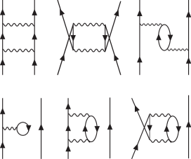
Figure 1: Valence-linked $\hat{Q}$-box diagrams up to second order in $V$.

At the end, we stress again that the above KK method can yield $V_{\mathrm{eff}}$ only for a degenerate model space. Suppose we are working with the harmonic oscillator shell model of ${}^{18}\mathrm{O}$, treating ${}^{16}\mathrm{O}$ as the core. If we take the $P$-space composed only of the degenerate $sd$-shell, the above KK method works well as shown by many applications (see for example Ref. HjorthJensen1995125 ). If, on the other hand, we take an enlarged $P$-space defined by the non-degenerate $sdf_{7}p_{3}$-shell, the KK method breaks down. A naive calculation of $V_{\mathrm{eff}}$ by Eq. (22) easily leads to divergences of the $\hat{Q}$-box, as we shall see later.

IV.3 Extended Kuo-Krenciglowa method

Here we derive the effective Hamiltonian $H_{\mathrm{eff}}$ of the Extended Kuo-Krenciglowa (EKK) method, with an emphasis on its similarity with the KK method discussed above.

IV.3.1 Derivation of the Extended Kuo-Krenciglowa method

We consider first the general situation where the energies of the valence single-particle states in $PH_{0}P$ are not necessarily degenerate. In this case, we have to apply the EKK formula Eq. (17) to our many-body systems.

We can easily confirm that, in order to derive Eq. (17), we need to change the decomposition Eq. (20) of the Hamiltonian in the KK method. Suppose we decompose the total Hamiltonian into the following unperturbed Hamiltonian $H^{\prime}_{0}$ and the perturbation $V^{\prime}$

$$H^{\prime}_{0} = PEP+QH_{0}Q$$

$$V^{\prime} = V-P(E-H_{0})P,$$ (25)

or in the matrix form,

$$H = H^{\prime}_{0}+V^{\prime}$$ (26)

$$= \begin{pmatrix}E&0\\ 0&QH_{0}Q\end{pmatrix}+\begin{pmatrix}P\tilde{H}P&PVQ\\ QVP&QVQ\end{pmatrix},$$

where $\tilde{H}\equiv H-E$, and $H_{0}=\sum\epsilon_{\alpha}a^{\dagger}_{\alpha}a_{\alpha}$. With the above unperturbed Hamiltonian $H^{\prime}_{0}$ in Eq. (25), we can treat the $P$-space as being degenerate at the energy $E$, and therefore we can follow the derivation of Eq. (22) in the KK method, to achieve

$$\tilde{H}_{\mathrm{eff}}=\tilde{H}_{\mathrm{BH}}(E)-\hat{Q^{\prime}}(E)\int\tilde{H}_{\mathrm{BH}}(E)+\hat{Q^{\prime}}(E)\int\tilde{H}_{\mathrm{BH}}(E)\int\tilde{H}_{\mathrm{BH}}(E)\cdots,$$ (27)

which is then converted into

$$\tilde{H}_{\mathrm{eff}}=\tilde{H}_{\mathrm{BH}}(E)+\frac{\mathrm{d}\hat{Q}(E)}{\mathrm{d}E}\tilde{H}_{\mathrm{eff}}+\frac{1}{2!}\frac{\mathrm{d}^{2}\hat{Q}(E)}{\mathrm{d}E^{2}}\{\tilde{H}_{\mathrm{eff}}\}^{2}+\cdots.$$ (28)

Note that Eqs. (27) and (28) are the EKK counterparts of Eqs. (22) and (24) of the KK method. We can solve Eq. (28) iteratively as done for Eq. (24).

Note that the above derivation of the EKK method is the same as that of the KK method apart from the decomposition of the Hamiltonian. Therefore, we need to retain only the valence-linked $\hat{Q}$-box diagrams in Eqs. (27) and (28), as we do for the KK method. To summarize, all that we have to know is, as in the KK method, the $\hat{Q}$-box and its energy derivatives, except that now it is defined at the parameter $E$.

IV.3.2 Perturbative expansion of the $\hat{Q}$-box

We discuss here how one can accommodate the perturbative expansion of the $\hat{Q}$-box in the EKK formalism. For the sake of simplicity, we will focus on a simple system composed of two particles on top of a closed-shell core in what follows, although the discussion is not restricted to this specific case. The projection operators $P$ and $Q$ are then given by

$$P=\sum_{a,b}a^{\dagger}_{a}a^{\dagger}_{b}\lvert c\rangle\langle c\rvert a_{b}a_{a},\,\,\,\,\,\,Q=1-P.$$ (29)

where $\lvert c\rangle$ stands for the closed-shell core.

To become familiar with our new unperturbed Hamiltonian, $H^{\prime}_{0}$, we consider some selected examples; we show first the results from the operation of the new unperturbed Hamiltonian, $H_{0}^{\prime}$, on some selected many-particle states:

$$H_{0}^{\prime}~{}a^{\dagger}_{a}a^{\dagger}_{b}\lvert c\rangle=E~{}a^{\dagger}_{a}a^{\dagger}_{b}\lvert c\rangle,$$

$$H_{0}^{\prime}~{}a^{\dagger}_{a}a^{\dagger}_{p}\lvert c\rangle=(\epsilon_{a}+\epsilon_{p})~{}a^{\dagger}_{a}a^{\dagger}_{p}\lvert c\rangle,$$ (30)

$$H_{0}^{\prime}~{}a^{\dagger}_{a}a^{\dagger}_{b}a^{\dagger}_{p}a_{h}\lvert c\rangle=(\epsilon_{a}+\epsilon_{b}+\epsilon_{p}-\epsilon_{h})~{}a^{\dagger}_{a}a^{\dagger}_{b}a^{\dagger}_{p}a_{h}\lvert c\rangle.$$

The first line is an example of a $P$-space state with two single-particle states on top of the closed-shell core, $|c\rangle$, while the second and third lines result in $Q$-space examples. The unperturbed energy of the $P$-space state $a^{\dagger}_{a}a^{\dagger}_{b}\lvert c\rangle$ is $E$, while that of a $Q$-space state $a^{\dagger}_{a}a^{\dagger}_{p}\lvert c\rangle$ results in $\epsilon_{a}+\epsilon_{p}$, a sum of unperturbed single-particle energies. It is important to get convinced that $\epsilon_{a}$ appears only in the $Q$-space energy, while $a^{\dagger}_{a}$ appears in all of the above three states.

In the perturbative expansion of $\hat{Q}(E)$ in Eq. (23), all the intermediate states are in the $Q$-space, and their unperturbed energies are given as in the second and third lines of the above example. The general structure of $\hat{Q}(E)$ can then be given schematically by

$$\hat{Q}(E)=\prod\frac{V}{E-(\sum\epsilon_{a}+\sum\epsilon_{p}-\sum\epsilon_{h})_{int}},{}$$ (31)

where the subscript $int$ indicates intermediate states between two interaction vertices. Note that the parameter $E$ appears in all the denominators in the EKK method.

Let us consider the $\hat{Q}$-box diagram shown in Fig. 2 as an example. The diagram is a contribution from the second-order term in Eq. (23), and gives the following contribution to $\hat{Q}(E)$

$$\mathrm{Fig.2(EKK)}\rightarrow\frac{V_{ah,cp}V_{pb,hd}}{E-\epsilon_{c}-\epsilon_{b}-\epsilon_{p}+\epsilon_{h}}.$$ (32)

If we on the other hand employ the KK method in order to calculate the contribution to $\hat{Q}(\epsilon_{0})$ from Fig. 2, we would get

$$\mathrm{Fig.2(KK)} \rightarrow \frac{V_{ah,cp}V_{pb,hd}}{(\epsilon_{c}+\epsilon_{d})-\epsilon_{c}-\epsilon_{p}+\epsilon_{h}-\epsilon_{b}}$$ (33)

$$= \frac{V_{ah,cp}V_{pb,hd}}{-\epsilon_{p}+\epsilon_{h}}$$

where, in going to the second line, we have used the fact that the $P$-space is degenerate, and therefore $\epsilon_{a}=\epsilon_{b}=\epsilon_{c}=\epsilon_{d}$ and $\epsilon_{c}+\epsilon_{d}=\epsilon_{0}$.

Two points should be noted from the above example; first, in a degenerate model space, the EKK result Eq. (32) with $E=\epsilon_{0}$ coincides with the KK result Eq. (33). This is a direct consequence of the fact that the EKK formula contains the KK formula as a special case. Second, we can see the problem of divergence of the KK formula applied naively to a non-degenerate model space. Consider the case of ${}^{18}\mathrm{O}$ as an example, and let the $P$-space consist of two major shells ($1s0d$ and $1p0f$-shells). Then, the denominator of the first line in Eq. (33) vanishes for $b,c,p\in 1s0d$-shell, $a,d\in 1p0f$-shell, and $h\in 0p$-shell, leading thereby to a divergence. The above mechanism is just one of many examples which show that we really need to use the EKK formalism in order to derive effective interactions for model spaces consisting of several shells.

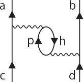
Figure 2: Core-polarization diagram as a second order in $V$ contribution to the $\hat{Q}$-box.

IV.3.3 The energy parameter $E$

Here we make several points in connection with the new parameter $E$ in the EKK theory.

First, by virtue of the arbitrariness of the parameter $E$, we can get around the problems of the poles of the $\hat{Q}$-box. As explained with the example in Fig. 2, the $\hat{Q}$-box contribution, (33), is divergent in the KK formula when we work in a non-degenerate model space. On the other hand, the EKK counterpart, (32), becomes divergent only for specific values of $E$. This means that we can always select a parameter $E$ that makes the $\hat{Q}$-box to behave smoothly as a function of $E$.

Second, the parameter $E$ provides us with a reasonable test of the calculation. Equation (19) shows that the resulting effective Hamiltonian $H_{\mathrm{eff}}$, does not depend on the value of $E$, provided that we have the exact $\hat{Q}$-box in Eq. (19). Any approximation may spoil the $E$-independence of $H_{\mathrm{eff}}$, and thereby of other physical quantities described by $H_{\mathrm{eff}}$. This may in turn imply that a $\hat{Q}$-box that gives $E$-independent physical quantities is a good approximation to the exact $\hat{Q}$-box. In the most sophisticated calculations up to date, we can evaluate the $\hat{Q}$-box diagrams only up to third order in the perturbation $V$ at most, and we can include only a limited number of excitations in the intermediate states (typically including up to $10-20$ oscillator quanta excitations), because of practical computational limitations. In Sec. V, we shall present numerical tests of the above $E$-independence.

Here we explain how to fix the value of $E$ in the actual calculations. If there are no intruder states in the target states $\{\lvert\phi_{i}\rangle,\,i=1,\cdots,d\}$ that are to be described by $H_{\mathrm{eff}}$, it can be shown that there is a finite range of $E$ values that make the series in Eq. (28) convergent Takayanagi201191 . The convergence is usually at its fastest when $E$ is fixed around the mean value of the target energies, $\{E_{i},\,i=1,\cdots,d\}$. Let us come back to our specific case of two particles on top of a core, and employ a single-particle basis of the harmonic oscillator. Let $\epsilon_{a}^{\mathrm{min}}$ be the minimum energy of active (valence) particle states. We then expect that our target states are distributed around $E\sim 2\epsilon_{a}^{\mathrm{min}}$, which serve as the first guess for $E$. It is also clear that the lowest energy of the $Q$-space states is $2\epsilon_{a}^{\mathrm{min}}+1\hbar\omega$, which gives the lowest position of the poles of $\hat{Q}(E)$.

In actual calculations, the allowed range of $E$, which is limited both from above and from below, can be estimated as follows. Let us increase $E$ from the above “optimal ” value $2\epsilon_{a}^{\mathrm{min}}$. As $E$ approaches the lowest pole $2\epsilon_{a}^{\mathrm{min}}+1\hbar\omega$ of $\hat{Q}(E)$, $\hat{Q}(E)$ and its derivatives in Eq. (28) would diverge. On the other hand, if we choose too low a value of $E\ll 2\epsilon_{a}^{\mathrm{min}}$, the resultant energy denominators in the $\hat{Q}(E)$ would be dominated by $E$, but not by the unperturbed energies of the intermediate states. In this situation, we have to expect that our approximation, truncation of the intermediate states at some unperturbed energies, cannot be justified.

In the next section, we present numerical examples where $E$ is varied in some range around $E\sim 2\epsilon_{a}^{\mathrm{min}}$.

V Numerical results

In order to apply the EKK formalism to nuclear systems, we consider simple nuclei composed of two nucleons on top of a given closed-shell core, ${}^{18}\mathrm{O},{}^{18}\mathrm{F}$ and ${}^{42}\mathrm{Ca},{}^{42}\mathrm{Sc}$, employing a single-particle basis defined by the harmonic oscillator unperturbed Hamiltonian. As the $P$-space for ${}^{18}\mathrm{O}$ and ${}^{18}\mathrm{F}$, we employ the $sd$-shell (degenerate case), and the $sdf_{7}p_{3}$-shell (non-degenerate case) composed of the $sd$ shell and the $0f_{7/2}$ and the $1p_{3/2}$ single-particle states. The $P$-space for ${}^{42}\mathrm{Ca},{}^{42}\mathrm{Sc}$ is the $pf$-shell (degenerate case), and the $pfg_{9}$-shell (non-degenerate case) composed of all the $pf$-shell single-particle states and the $0g_{9/2}$ single-particle state. In the degenerate $P$-space, both the KK and the EKK methods can be used, while in the non-degenerate $P$-space only the EKK method is applicable.

Our input interaction $V$ in the Hamiltonian Eq. (20) is the low-momentum interaction $V_{\mathrm{low}k}$ with a sharp cutoff $\Lambda=2.5~{}\mathrm{fm}^{-1}$, derived from the chiral $\chi$N³LO interaction of Entem and Machleidt entem2003 ; machleidt2011 . Our total $(P+Q)$ Hilbert space is composed of the harmonic oscillator basis states in the lowest seven major shells. The $Q$-space degrees of freedom come into play either by the KK method or the EKK method through the $\hat{Q}$-box that is calculated to third order in the interaction $V$. The final effective interactions are thus obtained in the $P$-space of one or two major shells.

We ought to mention two points. First, the amount of oscillator quanta excitations in each term in perturbation theory, may not be fully adequate if one is interested in final shell-model energies that are converged with respect to the number of intermediate excitations in the $\hat{Q}$-box diagrams. Second, neglected many-body correlations, like those arising from three-body forces are not taken into account. Such effects, together with other many-body correlations not included here are expected to play important roles, see for example the recent studies of neutron-rich oxygen and calcium isotopes PhysRevLett.105.032501 ; Holt:2010yb ; Otsuka:2013ig ; PhysRevLett.108.242501 ; PhysRevLett.109.032502 . However, the aim here is to study the effective interactions that arise from the KK and the EKK methods in one and two major shells. Detailed calculations for nuclei along various isotopic chains will be presented elsewhere.

In the actual calculation of the $\hat{Q}$-box using the harmonic oscillator basis functions, we drop the Hartree-Fock diagram contributions, assuming that it is well simulated by the harmonic oscillator potential, as in many of the former works HjorthJensen1995125 .

In order to show how the EKK method works, we present separate studies of (i) the two-body matrix elements (TBMEs) of the effective interaction $V_{\mathrm{eff}}$, and (ii) several energy levels obtained by shell model calculations. In particular, we focus on the $E$-independence of the numerical results; as discussed in Sec. II, the effective Hamiltonian $H_{\mathrm{eff}}$ obtained with the exact $\hat{Q}$-box is independent on the energy parameter $E$, and so are physical quantities calculated with $H_{\mathrm{eff}}$. In other words, the explicit $E$-dependence of the first term $H_{\mathrm{BH}}(E)$ (or equivalently $\hat{Q}(E)$) in Eq. (28) is canceled by other terms that represent the folded diagram contributions, making thereby $H_{\mathrm{eff}}$ (and therefore $V_{\mathrm{eff}}$) energy independent. In actual calculations, however, we can calculate the $\hat{Q}$-box only up to third order in $V$, and we have to examine the $E$-dependence of the right hand side of Eq. (19). In what follows, we shall see clearly that the $\hat{Q}$-box up to third order is sufficient to achieve an almost $E$-independent effective interaction $V_{\mathrm{eff}}$ (or $H_{\mathrm{eff}}$).

V.1 EKK method in $sd$-shell and $sdf_{7}p_{3}$-shell

In this section, we consider ${}^{18}\mathrm{O}$ and ${}^{18}\mathrm{F}$ as two-nucleon systems on top of the ${}^{16}\mathrm{O}$ closed-shell core. We calculate the effective interactions $V_{\mathrm{eff}}$ in the degenerate $sd$-shell, and in the non-degenerate $sdf_{7}p_{3}$-shell model spaces. The input of the EKK method is the $\hat{Q}$-box calculated up to third order in $V$ with the harmonic oscillator basis of $\hbar\omega=14~{}\mathrm{MeV}$. We set the origin of the energy as $\epsilon_{sd}=0$, which suggests that the optimal choice of $E$ is $E\sim 0$.

V.1.1 degenerate $sd$-shell model space

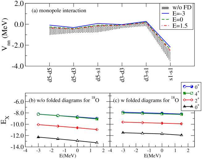
Figure 3: (Color online) $E$-dependence of the EKK results of neutron-neutron channel in the $sd$-shell (degenerate model space). The figure shows the monopole part, of $V_{\mathrm{eff}}$ (denoted by $\mathrm{V_{nn}}$), see Eq. (34), and the level energies of ${}^{18}\mathrm{O}$ with respect to ${}^{16}\mathrm{O}$. In panel (a), the monopole panel, dotted lines (which make the shaded area) show the results without the folded diagram contributions for $-3\leq E\leq 1.5~{}\mathrm{MeV}$. The full line, dashed line and dot-dash line show the $\mathrm{V_{nn}}$ for $E=-3,~{}0,~{}1.5~{}\mathrm{MeV}$, respectively. In the lower panels (b) and (c), energy levels are calculated for $E=-3,~{}-1.5,~{}0,~{}1.5~{}\mathrm{MeV}$ (b) without and (c) with the folded diagram contribution. Triangles, diamonds, squares and circles show the energy levels of the ground, the first excited, the second and third excited states, respectively.

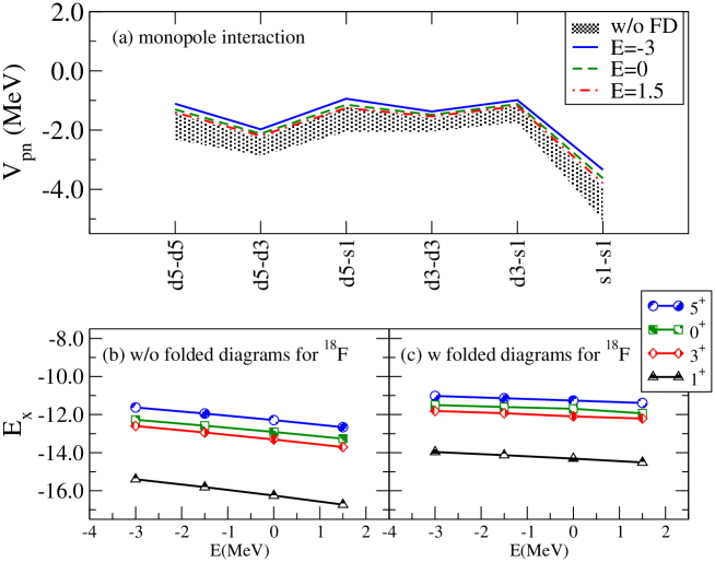
Figure 4: (Color online) $E$-dependence of the EKK results of proton-neutron channel in the $sd$-shell (degenerate model space). (a) monopole part of the interaction, (b) level energies of ${}^{18}\mathrm{F}$ without folded diagrams and (c) with folded diagrams. Else, we use the same notation as in Fig. 3.

In Fig. 3, we show our numerical results for the two-body matrix elements and level energies calculated in the degenerate $sd$-shell model space for the neutron-neutron channel (${}^{18}\mathrm{O}$) and in Fig. 4 the proton-neutron channel (${}^{18}\mathrm{F}$).

To see the $E$-independence of the numerical results for $V_{\mathrm{eff}}$, calculations are performed for several values of $E$. As explained before, the optimal value of $E$ may be estimated as $E\sim 2\epsilon_{sd}=0$. Note also that $E=0$ is far from the lowest pole of $\hat{Q}(E)$, $E=E_{\mathrm{pole}}^{min}=1~{}\hbar\omega=14~{}\mathrm{MeV}$, and the calculation is free from the divergence problem of the $\hat{Q}$-box. We have thus varied $E$ in the range of $-3\leq E\leq 1.5~{}\mathrm{MeV}$ in Fig. 3 and 4. Obviously, the EKK method with $E=0$ coincides exactly with the KK method because our $P$-space is degenerate now (compare Eqs. (32) and (33)).

In order to study the effect on the various matrix elements, we analyze the monopole term in the neutron-neutron channel in Fig. 3 (a). The monopole part of $V_{\mathrm{eff}}$, is defined as

$$V_{\mathrm{eff}}{}_{j,j^{\prime}}^{T}=\frac{\sum_{J}(2J+1)\langle jj^{\prime}\rvert V_{\mathrm{eff}}\lvert jj^{\prime}\rangle_{JT}}{\sum_{J}(2J+1)}.$$ (34)

Let us look at the dotted lines (which make a shaded band in the figure) that are calculated by dropping the folded diagram contributions, i.e., by replacing $V_{\mathrm{eff}}$ simply by $\hat{Q}(E)$. We can see clearly that $\hat{Q}(E)$ depends strongly on $E$. Next, let us turn to the EKK results that include all the folded diagram contributions in the right hand side of Eq. (28). They are shown by solid lines for $E=-3,~{}0,~{}1.5~{}\mathrm{MeV}$, whose difference can hardly be seen. The above observation suggests that the folded diagrams cancel the $E$-dependence of $\hat{Q}(E)$ and yield an almost $E$-independent $\tilde{H}_{\mathrm{eff}}$ (and $V_{\mathrm{eff}}$) in Eq. (28).

In the lower panels (b) and (c) of Fig. 3, we show several energy levels of ${}^{18}\mathrm{O}$ with respect to ${}^{16}\mathrm{O}$ obtained by shell-model calculations with our effective interaction $V_{\mathrm{eff}}$. Here the single particle energies in the shell-model diagonalization are taken from the USD interaction Brown:1988ff ; Brown1988191 ; the single-particle energies of the states (in the isospin formalism) $\epsilon_{d_{5/2}},~{}\epsilon_{s_{1/2}},$ and $\epsilon_{d_{3/2}}$ are $-3.9478$ MeV, $-3.1635$ MeV and $1.6466$ MeV, respectively.

Panels (b) and (c) show the results without and with folded diagram contributions, respectively. We note that in panel (b) the energy levels are decreasing functions of $E$, which is explained by the $E$-dependence of $\hat{Q}(E)$. On the other hand, in panel (c), we see that the energy levels are almost independent of the parameter $E$, as they should.

The above observation also implies that the evaluation of the $\hat{Q}$-box up to third order in $V$ is sufficient to establish a seemingly $E$-independence of the right hand side of Eq. (28), and therefore of $V_{\mathrm{eff}}$ in the left hand side.

Figure 4 shows the results for $V_{\mathrm{eff}}$ in the proton-neutron channel and level energies for ${}^{18}\mathrm{F}$ with the same setting as for ${}^{18}\mathrm{O}$. We can repeat exactly the same arguments as we did for ${}^{18}\mathrm{O}$ and realize that the folded diagram contribution eliminates the $E$-dependence, to a large extent, of $\hat{Q}(E)$ to give, almost, an $E$-independent $V_{\mathrm{eff}}$ and energy levels.

V.1.2 Non-degenerate $sdf_{7}p_{3}$-shell

Here we examine ${}^{18}\mathrm{O}$ and ${}^{18}\mathrm{F}$ in the non-degenerate $P$-space, labelled the $sdf_{7}p_{3}$-shell here, composed of the $sd$-shell and the $0f_{7/2}$ and $1p_{3/2}$ single-particle states. In this non-degenerate model space, the standard KK method cannot be applied, since it leads to divergences, as discussed above. The EKK method offers however a viable approach to this system. To date, therefore, there have been only empirical interactions in this model space, see for example the effective interaction employed in Ref. PhysRevC.60.054315 .

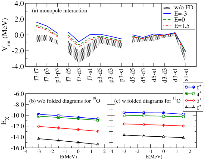
Figure 5: (Color online) $E$-dependence of the EKK results of neutron-neutron channel in the $sdf_{7}p_{3}$-shell (non-degenerate model space). (a) monopole part of the interaction, (b) level energies of ${}^{18}\mathrm{O}$ without folded diagrams and (c) with folded diagrams. Else, we use the same notation as in Fig. 3.

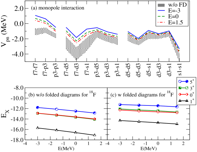
Figure 6: (Color online) $E$-dependence of the EKK results of proton-neutron channel in the $sdf_{7}p_{3}$-shell (non-degenerate model space). (a) monopole part of the interaction, (b) level energies of ${}^{18}\mathrm{F}$ without folded diagrams and (c) with folded diagrams. Else, we use the same notation as in Fig. 4.

Figures 5 and 6 show the numerical results of the EKK method in the $sdf_{7}p_{3}$ model space, in the same way as Figs. 3 and 4 for the degenerate $sd$-shell. In what follows, we will introduce the wording inter-shell interaction for the interaction between particles in different major shells, for example we can have one particle in the $sd$-shell and the other one in the $pf$-shell. Similarly, we will use the naming intra-shell interaction for interactions between particles within a single major shell.

Let us first study the the monopole part of the TBMEs of $V_{\mathrm{eff}}$ (Fig. 5 (a) for neutron-neutron channel and Fig. 6 (a) for proton-neutron channel). Here we have inter-shell interactions in addition to the intra-shell interactions within the $sd$-shell and within the $pf$-shell. We see that the inter-shell interactions depend more strongly on $E$ without the folded diagrams than the intra-shell interaction within the $sd$-shell. This feature is due to the fact that $\hat{Q}(E)$ for the inter-shell interaction has intermediate states with small energy denominators. This figure clearly shows that the folded diagram contributions cancel the strong $E$-dependence of the $\hat{Q}(E)$, and the resulting $V_{\mathrm{eff}}$ becomes almost independent of $E$, showing that the EKK method is stable and useful also in the non-degenerate $sdf_{7}p_{3}$-shell.

From the panels of the energy levels of ${}^{18}\mathrm{O}$ and ${}^{18}\mathrm{F}$, we can draw the same conclusion for the degenerate $sd$-shell; the folded diagram contribution makes the energy levels independent of the parameter $E$.

V.1.3 Comparison of KK and EKK methods

The main advantage of our EKK method is that it allows for a fully consistent treatment of the non-degenerate model space. On the other hand, in the KK method, the naive perturbative calculation of $\hat{Q}$-box by Eq. (22) leads to divergence in non-degenerate $sdf_{7}p_{3}$-shell, as discussed in Sec. IV.3.

One possible ad hoc way to avoid this divergence is to artificially force the $sdf_{7}p_{3}$-shell to be degenerate in energy by shifting the single-particle energies Holt:2010yb . Although there is no physical justification for this artificial shift, it removes the poles which arise in the various $\hat{Q}$-box diagrams.

Note, however, that the obtained $V_{\mathrm{eff}}$ is defined with artificially degenerate single-particle energies. Furthermore, in actual calculations, this method dose not necessarily lead to a convergent result even with all the folded diagrams in Eq. (22).

For the purpose of comparing the EKK method with the ad hoc treatment of the non-degeneracy in the KK method, we apply the EKK method to both sets of unperturbed Hamiltonians; one with the artificially degenerate $sdf_{7}p_{3}$-shell, and the other with the non-degenerate $sdf_{7}p_{3}$-shell. Note that the EKK method in the artificially degenerate $sdf_{7}p_{3}$-shell simulates the ad hoc KK method explained above. In this calculation, in order to obtain convergence, we set $E=-1.5$ MeV in both cases.

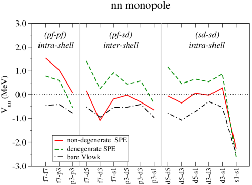
Figure 7: (Color online) The monopole part of $V_{\mathrm{eff}}$ in the $sdf_{7}p_{3}$ model space, obtained via the physical (non-degenerate) single particle energies (full line) and via the ad hoc (degenerate) single particle energies (dashed line). Both calculations are performed in the neutron-neutron channel. As a reference, the monopole part of the first-order effective is shown with dash-dotted line.

Figure 7 shows the monopole part of the effective interaction $V_{\mathrm{eff}}$ in the $sdf_{7}p_{3}$-shell interaction for the neutron-neutron channel. The dashed lines show the results with the ad hoc modification of the unperturbed Hamiltonian as explained above. The full lines display the results in the non-degenerate model space. To show the contribution of the $\hat{Q}$-box and folded diagrams, we display also the monopole part of the first-order term of the $\hat{Q}$-box. This term is energy independent.

It is interesting to note that the inter-shell (pf-sd) interaction and the intra-shell (sd-sd) interaction are more attractive in the EKK method than in the ad hoc KK method. This discrepancy clearly comes from the difference in the energy denominator in the $\hat{Q}$-box. Suppose we have two particles within $f_{7/2}$ or $p_{3/2}$ states. The magnitude of the energy denominator shown in Eq. (31) is larger, making thereby the $\hat{Q}$-box smaller in the EKK method than in the ad hoc KK method. For the inter-shell (pf-sd) interaction and the intra-shell (sd-sd) interaction, this difference makes the interaction for the artificially degenerate single-particle states more repulsive. On the other hand in the intra-shell (pf-pf) interaction, the EKK results are more repulsive than the ad hoc KK results. This can be understood as follows; the effect of the folded diagram contribution is quite large in the EKK method since we use $P\tilde{H}P$ in the folding procedure instead of $PVP$. This difference makes the contribution of the folded diagrams larger.

The above comparison shows that there is a sizable difference between the effective interaction in the EKK method and in the ad hoc KK method, and the difference affects mostly the inter-shell interaction.

V.2 EKK method in $pf$-shell and $pfg_{9}$-shell

We apply the EKK method to the nuclei ${}^{42}\mathrm{Ca}$ and ${}^{42}\mathrm{Sc}$ as well. These nuclei can be described as two nucleons on top of a ${}^{40}\mathrm{Ca}$ core. Here the degenerate model space is composed of the single-particle states of the $pf$-shell, while our non-degenerate model space is defined by the single-particle states of the $pf$-shell and the single-particle state $g_{09/2}$. We have performed the calculation in the same way as in Sec. V.1.2, but with an oscillator parameter $\hbar\omega=11~{}\mathrm{MeV}$, which is appropriate for ${}^{40}\mathrm{Ca}$ region. We have taken $\epsilon_{pf}=0$ and therefore our first guess for the energy parameter is $E=0$.

V.2.1 Results for $pf$-shell

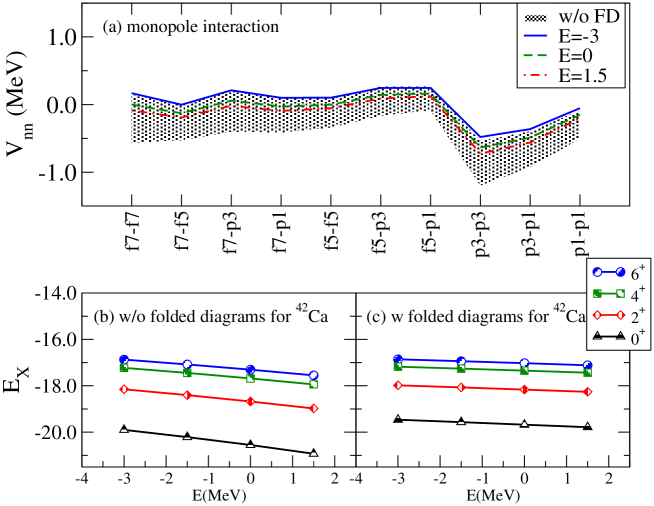
Figure 8: (Color online) $E$-dependence of the EKK results of neutron-neutron channel in the $pf$-shell (degenerate model space). (a) monopole part of the interaction, (b) level energies of ${}^{42}\mathrm{Ca}$ without folded diagrams and (c) with folded diagrams. Else, we use the same notation as in Fig. 3.

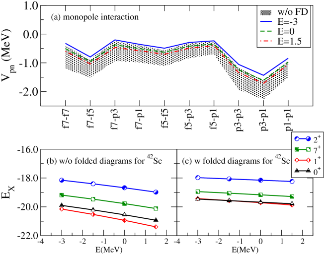
Figure 9: (Color online) $E$-dependence of the EKK results of proton-neutron channel in the $pf$-shell (degenerate model space). (a) monopole part of the interaction, (b) level energies of ${}^{42}\mathrm{Sc}$ without folded diagrams and (c) with folded diagrams. Else, we use the same notation as in Fig. 4.

Figure 8, 9 shows the effective interaction $V_{\mathrm{eff}}$ defined in the degenerate $pf$-shell. In Fig. 8, the panel (a) shows the neutron-neutron monopole interactions and the panels (b) and (c) display the energy levels of ${}^{42}\mathrm{Ca}$. Figure 9 shows the results for ${}^{42}\mathrm{Sc}$, the proton-neutron channel, in the same manner. In the shell-model diagonalization, the single particle energies are taken from the GXPF1 interaction PhysRevC.65.061301 ; the particle energies (in the isospin formalism) of $\epsilon_{f_{7/2}},~{}\epsilon_{p_{3/2}},~{}\epsilon_{p_{1/2}}$ and $\epsilon_{f_{5/2}}$ are equal to $-8.6240$ MeV, $-5.6793$ MeV, $-4.1370$ MeV and $-1.3829$ MeV, respectively.

We have carried out the calculation by varying $E$ in the range of $-3\leq E\leq 1.5~{}\mathrm{MeV}$. Clearly, we can make the same observation as in Sec. V.1.1; the shaded bands in the monopole panels shrink when we include folded diagrams, making the monopole part of $V_{\mathrm{eff}}$ almost independent of $E$. Moreover, from the energies levels of ${}^{42}\mathrm{Ca}$ (Fig. 8 (b) and (c)) and ${}^{42}\mathrm{Sc}$(Fig. 9 (b) and (c)), we observe that the folded diagrams restore nicely the $E$-independence of all the lowest-lying levels, which is a natural consequence expected by the theory.

V.2.2 Results for $pfg_{9}$-shell

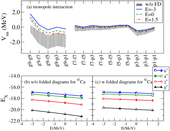
Figure 10: (Color online) $E$-dependence of the EKK results of neutron-neutron channel in the $pfg_{9}$-shell (non-degenerate model space). (a) monopole part of the interaction, (b) level energies of ${}^{42}\mathrm{Ca}$ without folded diagrams and (c) with folded diagrams. Else, we use the same notation as in Fig. 3.

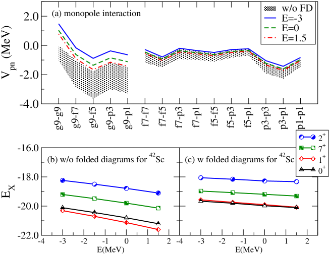
Figure 11: (Color online) $E$-dependence of the EKK results of proton-neutron channel in the $pfg_{9}$-shell (non-degenerate model space). (a) monopole part of the interaction, (b) level energies of ${}^{42}\mathrm{Sc}$ without folded diagrams and (c) with folded diagrams. Else, we use the same notation as in Fig. 4.

As our final example, we present the results for the $pfg_{9}$-shell in Fig. 10 for the neutron-neutron channel and Fig. 11 for the proton-neutron channel. The parameter $E$ is varied in the range of $-3\leq E\leq 1.5~{}\mathrm{MeV}$. The particle energies (in the isospin formalism) of $\epsilon_{f_{7/2}},~{}\epsilon_{p_{3/2}},~{}\epsilon_{p_{1/2}},~{}\epsilon_{f_{5/2}}$ and $\epsilon_{g_{9/2}}$ are equal to $-8.6240$ MeV, $-5.6793$ MeV, $-4.1370$ MeV, $-1.3829$ MeV and $2.1000$ MeV, respectively. We note again the role played by folded diagrams; they remove the $E$-dependence of the $\hat{Q}(E)$, resulting in an almost $E$-independent effective interaction $V_{\mathrm{eff}}$ and energy levels of ${}^{42}\mathrm{Ca}$ (Fig. 10 (b) and (c)) and ${}^{42}\mathrm{Sc}$ (Fig. 11 (b) and (c)).

V.3 Application of the EKK method to shell-model calculations

With effective Hamiltonians derived by the EKK method, we can study the role of such Hamiltonians in actual shell-model calculations. Here we focus on the previously discussed systems, with at most two valence nucleons outside a closed-shell core. Results from large-scale shell model calculations will be presented elsewhere.

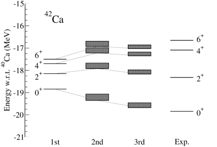
Figure 12: Energy levels of the ground state and low-lying states of ${}^{42}\mathrm{Ca}$ using the $\hat{Q}$-box to first, second, and third order in the interaction. The right most levels represent the experimental values. Energies are measured from the closed-shell core, ${}^{40}\mathrm{Ca}$. The TBMEs (neutron-neutron channel) are obtained by the EKK method, with the parameter $E$ in the range $-3\leq E\leq 0$ MeV. The shaded bands indicate the variation of calculated energy levels for $-3\leq E\leq 0$ MeV.

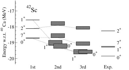
Figure 13: Energy levels of the ground state and low-lying states of ${}^{42}\mathrm{Sc}$ with respect to ${}^{40}\mathrm{Ca}$ core. The TBMEs (proton-neutron channel) are obtained via EKK method with parameter $-3\leq E\leq 0$ MeV. Since we do not include Coulomb effects throughout the calculation, the absolute values are shifted by $-7.2$ MeV, so that the $0^{+}$ state forms the $T=1$ triplet state with the corresponding $0^{+}$ ground state of ${}^{42}\mathrm{Ca}$. Other notation is the same as for Fig. 12.

For this purpose, Fig. 12 shows the low-lying energy levels for ${}^{42}\mathrm{Ca}$ obtained by the shell-model calculation with the same setting as in Sec. V.2.1. The TBMEs are derived by the EKK method, with the $\hat{Q}$-box calculated to first, second and third order in the interaction $V$. The parameter $E$ is varied in the range of $-3\leq E\leq 0$ MeV in the calculation of the second-order and the third-order $\hat{Q}$-box. Note that the first-order $\hat{Q}$-box is $V$ itself, and is independent of $E$. The leftmost levels show the result with the first-order $\hat{Q}$-box. The middle two levels represent the results with the second-order and third-order $\hat{Q}$-box, where the shaded bands show the range of the energy levels corresponding to $-3\leq E\leq 0~{}\mathrm{MeV}$. The rightmost levels are the experimental data.

As discussed above, by construction, all the physical results are independent of $E$ if our $\hat{Q}$-box is calculated without any approximation. In other words, the weaker dependence on $E$ implies a better approximation to the $\hat{Q}$-box (see Figs. 3-6, 8-11). This means that the width of the shaded band may be taken as a measure of the size of the error.

In Fig. 12, independently of the comparison to experiment, two types of convergence can be seen; the first one is (i) the convergence of the energy levels with respect to the order of the perturbation, and the second one is (ii) the convergence of the band widths ($E$-dependence of the energy levels) with respect to the order of the perturbation.

Let us start with discussions on the convergence issue (i). Figure 12 shows that the magnitude of the third-order contribution is approximately 30% as large as that of the second-order contribution. A simple estimate from these observations tells us that the perturbation series make a geometric series with common ratio $\sim 0.3$. We can then expect that the fourth-order correction to the $\hat{Q}$-box are small.

Let us turn to the convergence case (ii). Figure 12 exhibits also that, compared with the second-order $\hat{Q}$-box, the band widths are smaller for the third-order $\hat{Q}$-box, as we would expect. Besides these theoretical features, the agreement with experiment is acceptable.

Next we examine the proton-neutron channel using ${}^{42}\mathrm{Sc}$ as our testcase. The results are shown in Fig. 13. The experimental values (right-most levels) are shifted by $-7.2~{}\mathrm{MeV}$ so that the $0^{+}$ state forms the $T=1$ triplet state with corresponding $0^{+}$ ground state of ${}^{42}\mathrm{Ca}$, since we presently do not take into account any isospin dependence of the nuclear force or the Coulomb interaction.

Here we observe similar patterns to those seen in the neutron-neutron channel of Fig. 12. However, we notice that as far as the convergence case (i) is concerned, the contribution of third-order terms is not necessarily smaller than second-order contributions.

On the other hand, for the convergence case (ii), we observe smaller band widths for the third-order $\hat{Q}$-box results as compared with those obtained with the second-order $\hat{Q}$-box. This may indicate that the third-order $\hat{Q}$-box represents a better approximation than the second-order $\hat{Q}$-box.

The agreement with experimental data is rather nice for the $0^{+},7^{+},3^{+}$ states, but we observe a slight overbinding for the $1^{+}$ state. From the convergence property of the $1^{+}$ state, it is unlikely that fourth-order contributions to the $\hat{Q}$-box could play an important role. Several explanations for this discrepancy are possible. One possibility for this overbinding is that the single particle energies presently used are not fully adequate. As mentioned above, we have employed the single-particle energies determined from the GXPF1 PhysRevC.65.061301 interaction. These energies are the results of a fit together with the two-body interaction to reproduce experimental data. The experimental data that enter the fitting procedure consist of selected observables from $pf$-shell nuclei. Since the GXPF1 interaction differs from those derived here, other sets of single-particle energies could have been more appropriate. Another possibility is that our $Q$-space and order in perturbation theory may not be large enough. Thus, there may be missing many-body correlations which could play an important role. Three-body forces PhysRevLett.105.032501 ; Holt:2010yb ; Otsuka:2013ig ; PhysRevLett.108.242501 ; PhysRevLett.109.032502 are examples of many-body contributions not studied here. However, the aim of this work has been to study the recently developed EKK formalism for deriving effective interactions for more than one major shell. The role of more complicated many-body correlations are the scope of future works.

VI Conclusion

We have presented a novel many-body theory (the so-called EKK method) to calculate the effective interaction $V_{\mathrm{eff}}$ for the shell-model calculation that is applicable not only to degenerate model spaces, but also to non-degenerate model spaces. The method is based on a re-interpretation of the unperturbed Hamiltonian and the interacting part. The final expressions for the effective interactions can be understood as a Taylor series expansion of the Bloch-Horowitz Hamiltonian around a newly introduced parameter $E$. Since the change in $E$ should not affect the effective interactions $V_{\mathrm{eff}}$, the $E$-independence of the numerical results provides us with a sensible test of our framework and the approximations we make in the actual calculations.

In this work, we have presented numerical results for the effective two-body nucleon-nucleon interactions $V_{\mathrm{eff}}$, with applications to shell-model calculations of selected nuclei, with and without the contribution from the folded diagrams. The degenerate model spaces are the $sd$-shell for the nuclei ${}^{18}\mathrm{O}$ and ${}^{18}\mathrm{F}$, and the $pf$-shell for the nuclei ${}^{42}\mathrm{Ca}$ and ${}^{42}\mathrm{Sc}$. Our non-degenerate model spaces consist of the single-particle states from the $sdf_{7}p_{3}$-shell and the $pfg_{9}$-shell. Based on our numerical results, we have found that our method works well in practical situations. For degenerate model spaces, our method gives the same results as the conventional KK method. In the non-degenerate model space, which is beyond the applicability of the KK method, we have shown that our method works nicely.

Second, we have shown that our $V_{\mathrm{eff}}$ and therefore the energy levels are almost independent of the parameter $E$, as they should, if we calculate the $\hat{Q}$-box up to third order. This in turn suggests that the perturbative expansion of the $\hat{Q}$-box through third order gives almost converged results.

Third, the difference between the EKK method and the KK method with an ad hoc modification of the unperturbed Hamiltonian is significant, especially for inter-shell interactions. This can have a large impact, for example, on the investigation of neutron-rich nuclei where the degrees of freedom defined by two or more major oscillator shells are important.

Finally, we stress that our method has established a robust way to calculate microscopically the effective interaction in non-degenerate model spaces. These spaces involve typically more than one major oscillator shell. We believe that this is an indispensable step to make the nuclear shell model a reliable theory, in particular for exotic nuclei, based on a microscopic effective interaction derived from the realistic nucleon-nucleon interactions.

VII Acknowledgments

We thank Gaute Hagen and Koshiroh Tsukiyama for fruitful discussions. This work is supported in part by Grant-in-Aid for Scientific Research (A) 20244022 and also by Grant-in-Aid for JSPS Fellows (No. 228635), by the JSPS Core to Core program “International Research Network for Exotic Femto Systems” (EFES), and the high-performance computing project NOTUR in Norway. This work was supported by the Research Council of Norway under contract ISP-Fysikk/216699.

References

- (1) B. A. Brown, W. A. Richter, R. E. Julies and B. H. Wildenthal, Ann. Phys. 182, 191 (1988).
- (2) M. Honma, T. Otsuka, B. A. Brown and T. Mizusaki, Phys. Rev. C 65, 061301 (2002).
- (3) Y. Utsuno, T. Otsuka, T. Glasmacher, T. Mizusaki and M. Honma, Phys. Rev. C 70, 044307 (2004).
- (4) A. Poves and A. Zuker, Phys. Rep. 70, 235 (1981).
- (5) A. Poves, J. Sánchez-Solano, E. Caurier and F. Nowacki, Nucl. Phys. A 694, 157 (2001).
- (6) K. Takayanagi, Nucl. Phys. A 852, 61 (2011).
- (7) K. Takayanagi, Nucl. Phys. A 864, 91 (2011).
- (8) P. Navrátil, S. Quaglioni, I. Stetcu and B. R. Barrett, J. Phys. G 36, 083101 (2009).
- (9) B. R. Barrett, P. Navrátil, and J. P. Vary, Prog. Part. Nucl. Phys. 69, 131 (2013).
- (10) E. D. Jurgenson, P. Maris, R. J. Furnstahl, P. Navrátil, W. E. Ormand, and J. P. Vary, Phys. Rev. C 87, 054312 (2013).
- (11) M. Hjorth-Jensen, T. T. S. Kuo and E. Osnes, Phys. Rep. 261, 125 (1995).
- (12) T. T. S. Kuo and E. Osnes, Lecture Notes in Physics 364, Springer (1990).
- (13) E. M. Krenciglowa and T. T. S. Kuo, Nucl. Phys. A 235, 171 (1974).
- (14) K. Suzuki and S. Y. Lee, Prog. Theor. Phys. 64, 2091 (1980).
- (15) B. H. Brandow, Rev. Mod. Phys. 39, 771 (1968).
- (16) D. R. Entem and R. Machleidt, Phys. Rev. C 68, 041001(R) (2003).
- (17) R. Machleidt and D. R. Entem, Phys. Rep. 503, 1 (2011).
- (18) T. Otsuka, T. Suzuki, J. D. Holt, A. Schwenk and Y. Akaishi, Phys. Rev. Lett. 105, 032501 (2010).
- (19) J. D. Holt, T. Otsuka, A. Schwenk and T. Suzuki, J. Phys. G 39, 085111 (2012).
- (20) T. Otsuka and T. Suzuki, Few-Body Syst. 54, 891 (2013).
- (21) G. Hagen, M. Hjorth-Jensen, G. R. Jansen, R. Machleidt and T. Papenbrock, Phys. Rev. Lett. 108, 242501 (2012).
- (22) G. Hagen, M. Hjorth-Jensen, G. R. Jansen, R. Machleidt and T. Papenbrock, Phys. Rev. Lett. 109, 032502 (2012).
- (23) B. A. Brown and B. H. Wildenthal, Annu. Rev. Nucl. Part. Sci. 38, 29 (1988).
- (24) Y. Utsuno, T. Otsuka, T. Mizusaki and M. Honma, Phys. Rev. C 60, 054315 (1999).