Spatiotemporal Binary Interaction and Designer quasi particle Condensates

Abstract

We introduce a new integrable model to investigate the dynamics of two component quasi particle condensates with spatio temporal interaction strengths. We derive the associated Lax-pair of the coupled GP equation and construct matter wave solitons. We show that the spatio temporal binary interaction strengths not only facilitate the stabilization of the condensates, but also enables one to fabricate condensates with desirable densities, geometries and properties leading to the so called ”designer quasi particle condensates”.

Keywords:Gauge transformation; Bright soliton;GP equation.

1 Introduction

The experimental observation of Bose-Einstein condensates (BEC) in rubidium by Cornell and Wieman [1] and in sodium by Ketterle’s group [2] have signalled a new era in ultra cold atomic physics and have virtually opened the flood gates for matter wave manipulation. At ultra low temperatures, the behaviour of BECs is governed by the Gross-Pitaevskii (GP) equation which is nothing but the inhomogeneous (3+1) dimensional nonlinear Schrödinger (NLS) equation of the following form [3-6]

$$i\hbar\frac{\partial\psi(\vec{r},t)}{\partial t}=\left(-\frac{\hbar^{2}}{2m}\nabla^{2}+U|{\psi(\vec{r},t)}|^{2}+V(\vec{r},t)\right){\psi(\vec{r},t)},$$ (1)

where $U(\vec{r},t)$ describes the interatomic interaction and $V(\vec{r},t)$ represents the external trapping potential that traps the atoms at such low temperatures. Eventhough the above (3+1) dimensional GP equation is in general nonintegrable, it has been shown to admit integrability in quasi one dimensions for both time independent [7,8] and time dependent [9,10] harmonic trapping potentials. The experimental observation of bright [11-13] and dark solitons [14,15] in such quasi one dimensional BECs has not only reconfirmed the integrability of the associated dynamical systems, but also stimulated a lot of interest to get a deeper understanding of the nonlinear phenomena surrounding BECs.

    It must be mentioned that the behaviour of single component BECs is controlled by the external trapping potential and the binary interatomic interaction (scattering length). In contrast to single component BECs, the dynamics of multicomponent BECs [16-19] which comprise of either mixtures of different hyperfine states of the same atomic species or even mixtures of different atomic species is much richer by virtue of both interspecies interaction and intraspecies interaction. Multicomponent BECs show several interesting and novel phenomena like soliton trains, multidomain walls, spin switching [20], multi mode collective excitations etc., which are not normally encountered in single component BECs. The recent analytical investigations of multicomponent BECs [21,22] involving temporal variation of both interspecies and intraspecies scattering lengths have shown how the concept of coherent storage and matter wave switching can be manifested in the collisional dynamics of bright solitons.

    It is worth pointing at this juncture that the above scalar and vector BECs involve the condensation of atoms or particles with integral spin (bosons) at the ground state. Since the temperature at which bosons condense is governed by the inverse of the mass, the low density of the weekly interacting atoms combined with their relatively large mass ensures that the critical temperature is extremely low of the order order $10^{-6}k$. In this context, it was believed that the condensation of quasi particles like excitons and polaritons with their high densities and negligible masses might occur at temperatures of several orders of magnitude higher than for atoms, reachable by standard cryogenic techniques. In this connection, the advent of exciton BEC [23] and a polariton BEC (or) polariton laser[24] have certainly contributed to a resurgence in this exotic state of matter and have heralded a new era in semiconductor heterostructures. Excitons and polaritons are endowed with the spatially varying masses which ensures that the inter quasi-particle interaction could be spatially inhomogeneous. Recently, such quasi particle condensates were modelled [25] by the Gross- Pitaeveskii equation with a space dependent dispersion coefficient reperesenting the position dependent masses of quasi particles of the form

$$iq_{t}+k(x)q_{xx}+a(x)|q|^{2}q+v(x)q=0$$ (2)

In the above equation, the dispersion coefficient $k(x)$, the scattering length $a(x)$ and the trap $v(x)$ are related by the following equations

$$k(x)=\frac{4}{a(x)^{2}}$$ (3)

and

$$v(x)=\frac{-3a^{\prime}(x)^{2}+2a(x)a^{\prime\prime}(x)}{a(x)^{4}}.$$ (4)

   It should be mentioned that eq.(2) has been mapped on to the well known NLS equation and has been investigated earlier [26-31]. In this context, it would be interesting to investigate the dynamics of two component quasi particle condensates. The fact that the two component quasi particle condensates are endowed with both intraspecies interaction and interspecies interaction means that one could conceive of spatio temporal binary interaction in them.

   Motivated by the above consideration, we investigate the dynamics of two component quasi particle condensates with space and time modulated nonlinearities. In particular, we derive the lax pair of the associated Gross-Pitaeveskii equation and generate bright solitons. We also study the collisional dynamics of matter wave solitons in harmonic and optical lattice potentials.

2 Model and Lax-pair

   Considering a temporally and spatially inhomogeneous two component quasi particle BEC, the behaviour of the condensates that are prepared in two hyperfine states of the same atom can be described by the two coupled GP equation of the following form

$$i\psi_{1}(x,t)_{t} + k(x)\psi_{1}(x,t)_{xx}+\frac{2}{\sqrt{k(x)}}(A_{1}(t)^{2}|\psi_{1}(x,t)|^{2}$$ (5)

$$+ A_{2}(t)^{2}|\psi_{2}(x,t)|^{2})\psi_{1}(x,t)+(V(x,t)+i\frac{A_{1}(t)_{t}}{A_{1}(t)}$$

$$-\frac{i}{2}{b_{1}(t)}-\theta_{1}(t)_{t})\psi_{1}(x,t)=0,$$

$$i\psi_{2}(x,t)_{t} + k(x)\psi_{2}(x,t)_{xx}+\frac{2}{\sqrt{k(x)}}(A_{1}(t)^{2}|\psi_{1}(x,t)|^{2}$$ (6)

$$+ A_{2}(t)^{2}|\psi_{2}(x,t)|^{2})\psi_{2}(x,t)+(V(x,t)+i\frac{A_{2}(t)_{t}}{A_{2}(t)}$$

$$-\frac{i}{2}{b_{1}(t)}-\theta_{2}(t)_{t})\psi_{2}(x,t)=0,$$

where

$$V(x,t)=\frac{3}{16}\frac{k_{x}^{2}}{k}-\frac{1}{4}k_{xx}+\frac{1}{4}K^{2}{b_{1}}^{2}-\frac{1}{4}K^{2}{b_{1}}_{t}-{b_{0}}K,$$ (7)

and

$$K(x)=\int\frac{1}{{\sqrt{k(x)}}}dx.$$ (8)

In the above equation, $A_{1}(t),A_{2}(t),b_{0}(t),b_{1}(t),\theta_{1}(t)$ and $\theta_{2}(t)$ are arbitrary functions of time. The arbitrary functions $A_{1}(t)$and $A_{2}(t)$ describe the temporal variation of binary interaction while the arbitrary functions ($b_{0}(t),b_{1}(t)$) and ($\theta_{1}(t),\theta_{2}(t)$) facilitate us to choose the potential and atomic feeding respectively. In the above equation, the condensate wave functions are normalized to particle numbers $N_{i}=\int|\psi_{i}|^{2}d^{3}r$ while $k(x)$ which represents the spatially varying dispersion coefficient is also related to the mass of the quasi-particles. Equations (5) and (6) admit the following Lax-pair

$$\Phi_{x} + U\Phi=0,$$ (9)

$$\Phi_{t} + V\Phi=0,$$ (10)

where $\Phi=(\phi_{1},\phi_{2},\phi_{3})^{T}$ and

$$U = \left(\begin{array}[]{ccc}\frac{i}{2}\lambda&\frac{\psi_{1}}{k^{3/4}}&\frac{\psi_{2}}{k)^{3/4}}\\ -\frac{\psi_{1}^{*}}{k^{3/4}}&-\frac{i}{2}\lambda&0\\ -\frac{\psi_{2}^{*}}{k^{3/4}}&0&-\frac{i}{2}\lambda\\ \end{array}\right),$$ (14)

$$V = \left(\begin{array}[]{ccc}V_{11}&V_{12}&V_{13}\\ V_{21}&V_{22}&V_{23}\\ V_{31}&V_{32}&V_{33}\\ \end{array}\right),$$ (18)

with

$$V_{11} = -i\frac{\psi_{1}\psi_{1}^{*}}{{\sqrt{k}}}-i\frac{\psi_{2}\psi_{2}^{*}}{{\sqrt{k}}}+\frac{i}{2}\lambda^{2}k+ig;V_{12}=\chi_{1}+\lambda k^{1/4}\psi_{1},V_{13}=\chi_{2}+\lambda k^{1/4}\psi_{2},$$

$$V_{21} = -\chi_{1}^{*}-\lambda k^{1/4}\psi_{1}^{*},V_{22}=i\frac{\psi_{1}\psi_{1}^{*}}{{\sqrt{k}}}-\frac{i}{2}\lambda^{2}k-ig;V_{23}=i\frac{\psi_{2}\psi_{1}^{*}}{{\sqrt{k}}},$$

$$V_{31} = -\chi_{2}^{*}-\lambda k^{1/4}\psi_{2}^{*};V_{32}=i\frac{\psi_{2}^{*}\psi_{1}}{{\sqrt{k}}};V_{33}=i\frac{\psi_{2}\psi_{2}^{*}}{{\sqrt{k}}}-\frac{i}{2}\lambda^{2}k-ig,$$

$$\chi_{1} = \frac{-\frac{i}{4}\psi_{1}k_{x}}{k^{3/4}}+ik^{1/4}\psi_{1x},\chi_{1}^{*}=\frac{\frac{i}{4}\psi_{1}k_{x}}{k^{3/4}}-i^{1/4}\psi_{1x}^{*},$$

$$\chi_{2} = \frac{-\frac{i}{4}\psi_{2}k_{x}}{k^{3/4}}+ik^{1/4}\psi_{2x},\chi_{2}^{*}=\frac{\frac{i}{4}\psi_{2}k_{x}}{k^{3/4}}-ik^{1/4}\psi_{2x}^{*},$$

$$g(x) = {1\over 8}(b_{1t}-b_{1}^{2})K^{2}+{1\over 2}b_{0}K.$$ (19)

In the above equation, $\lambda(x,t)=\frac{b_{1}(t)K(x)/2+\Lambda(t)}{\sqrt{k(x)}}$ represents the complex nonisospectral parameter and $\Lambda(t)=\int{b_{0}(t)}e^{(-\int{b_{1}(t)}dt)dt+\mu)}e^{(\int{b_{1}(t)}dt)}$ is a complex function of time while $\mu$ is the so called ” hidden complex spectral parameter ”. The temporal scattering lengths have been absorbed into $\psi_{1}(x,t)$ and $\psi_{2}(x,t)$ by substituting $\psi_{1}(x,t)\rightarrow A_{1}(t)e^{i\theta_{1}(t)}\hat{\psi}_{1}(x,t)$ and $\psi_{2}(x,t)\rightarrow A_{1}(t)e^{i\theta_{1}(t)}\hat{\psi}_{2}(x,t)$. Under the following transformation

$$q_{1}(X,T) = A_{1}(t){\rm exp}\left(i\theta_{1}(t)-i\Pi\right)k(x)^{-1/4}I^{-1}\psi_{1}(x,t),$$

$$q_{2}(X,T) = A_{2}(t){\rm exp}\left(i\theta_{2}(t)-i\Pi\right)k(x)^{-1/4}I^{-1}\psi_{2}(x,t),$$ (20)

where

$$X = IK(x)+2\int I^{2}Jdt,$$

$$T = \int I^{2}dt,$$

$$I = {\rm exp}\left(\int b_{1}(t)dt\right),$$

$$J = \int b_{0}(t){\rm exp}\left(-\int b_{1}(t)dt\right)dt,$$

$$\Pi = -IJK(x)-{1\over 4}b_{1}(t)K(x)^{2}-\int I^{2}J^{2}dt,$$

eqs.(5) and (6) transform to the standard 2-component NLS equation [32].

3 Construction of Bright Vector Solitons

To generate the bright vector solitons of the coupled GP equations $(5)$ and $(6)$, we now consider the vacuum solution ($\psi_{1}^{0}=\psi_{2}^{(0)}=0$) so that the corresponding eigenvalue problem becomes

$$\Phi_{x}^{(0)}+U^{(0)}\Phi^{(0)}=0,$$ (21)

$$\Phi_{t}^{(0)}+V^{(0)}\Phi^{(0)}=0,$$ (22)

where

$$U^{(0)}=\left(\begin{array}[]{ccc}\frac{i}{2}\lambda(x,t)&0&0\\ 0&-\frac{i}{2}\lambda(x,t)&0\\ 0&0&-\frac{i}{2}\lambda(x,t)\\ \end{array}\right),$$ (23)

$$V^{(0)}=\left(\begin{array}[]{ccc}\frac{i}{2}\lambda^{2}k(x)&0&0\\ 0&-\frac{i}{2}\lambda^{2}k(x)&0\\ 0&0&-\frac{i}{2}\lambda^{2}k(x)\end{array}\right).$$

Solving the above eigenvalue problem, one obtains the following vacuum eigen function

$$\Phi^{(0)}=\left(\begin{array}[]{ccc}\phi^{(0)11}&0&0\\ 0&\phi^{(0)22}&0\\ 0&0&\phi^{(0)33}\\ \end{array}\right),$$ (24)

where

$$\phi^{(0)11} = e^{-\frac{i}{2}(b_{1}(t)K(x)^{2}/4+\Lambda(t)K(x)+\int\Lambda(t)^{2}dt)},$$

$$\phi^{(0)22} = e^{\frac{i}{2}(b_{1}(t)K(x)^{2}/4+\Lambda(t)K(x)+\int\Lambda(t)^{2}dt)},$$

$$\phi^{(0)33} = e^{\frac{i}{2}(b_{1}(t)K(x)^{2}/4+\Lambda(t)K(x)+\int\Lambda(t)^{2}dt)}.$$

We now gauge transform the vacuum eigenfunction $\Phi^{(0)}$ by a transformation function $g(x,t)$ to give

$$U^{(1)}=gU^{(0)}g^{-1}+g_{x}g^{-1},$$ (25)

$$V^{(1)}=gV^{(0)}g^{-1}+g_{t}g^{-1}.$$ (26)

We now choose the transformation function $g(x,t)$ from the solution of the associated Riemann problem such that it is meromorphic in the complex $\lambda$ plane as

$$g(x,t;\lambda)=\left[1+\frac{\lambda_{1}-\bar{\lambda}_{1}}{\lambda-\lambda_{1}}P(x,t)\right]\cdot\left(\begin{array}[]{ccc}1&0&0\\ 0&-1&0\\ 0&0&-1\\ \end{array}\right).$$ (27)

The inverse of matrix $g$ is given by

$$g^{-1}(x,t;\lambda)=\left(\begin{array}[]{ccc}1&0&0\\ 0&-1&0\\ 0&0&-1\\ \end{array}\right)\cdot\left[1-\frac{\lambda_{1}-\bar{\lambda}_{1}}{\lambda-\bar{\lambda}_{1}}P(x,t)\right]$$ (28)

where $\lambda_{1}$ and $\bar{\lambda}_{1}=\lambda_{1}^{*}$ are arbitrary complex parameters and $P$ is a 3$\times$3 projection matrix ($P^{2}=P$) which can be obtained using vacuum eigen function $\phi^{0}(x,t)$ as [33]

$$P=J\cdot\tilde{P}\cdot J,$$ (29)

where

$$\tilde{P}=\frac{M^{(1)}}{\rm{Trace}[M^{(1)}]},$$ (30)

$$J=\left(\begin{array}[]{ccc}1&0&0\\ 0&-1&0\\ 0&0&-1\\ \end{array}\right).$$ (31)

and

$$M^{(1)}=\Phi^{(0)}(x,t,\bar{\lambda}_{1})\cdot\hat{m}^{(1)}\cdot\Phi^{(0)}(x,t,\lambda_{1})^{-1}.$$ (32)

In the above equation, $\hat{m}^{(1)}$ is a 3$\times$3 arbitrary matrix taking the following form

$$\hat{m}^{(1)}=\left(\begin{array}[]{ccc}e^{2\delta_{1}}\sqrt{2}&\varepsilon_{1}^{(1)}e^{2i\eta_{1}}&\varepsilon_{2}^{(1)}e^{2i\eta_{1}}\\ \varepsilon_{1}^{*(1)}e^{-2i\eta_{1}}&e^{-2\delta_{1}}/\sqrt{2}&0\\ \varepsilon_{2}^{*(1)}e^{-2i\eta_{1}}&0&e^{-2\delta_{1}}/\sqrt{2}\\ \end{array}\right),$$ (33)

such that the determinant $M^{(1)}$ becomes zero with the condition $|\varepsilon_{1}^{(1)}|^{2}+|\varepsilon_{2}^{(1)}|^{2}$=$cos(\phi)^{2}+sin(\phi)^{2}$=1. Thus, choosing $\lambda_{1}=\alpha_{1}+i\beta_{1}$ and $\bar{\lambda}_{1}=\lambda_{1}^{*}$ and using eq. (26), the matrix $M^{(1)}$ can be explicitly written as

$$M^{(1)}=\left(\begin{array}[]{ccc}e^{-\Theta_{1}}\sqrt{2}&e^{-i\xi_{1}}\varepsilon_{1}^{(1)}&e^{-i\xi_{1}}\varepsilon_{2}^{(1)}\\ e^{i\xi_{1}}\varepsilon_{1}^{*(1)}&e^{\Theta_{1}}/\sqrt{2}&0\\ e^{i\xi_{1}}\varepsilon_{2}^{*(1)}&0&e^{\Theta_{1}}/\sqrt{2}\\ \end{array}\right),$$ (34)

where

$$\Theta_{1} = -\beta_{1}(t)K(x)-2\int\alpha_{1}(t)\beta_{1}(t)dt-2\delta_{1},$$ (35)

$$\xi_{1} = -b_{1}(t)K(x)^{2}/4-\alpha_{1}(t)K(x)$$ (36)

$$-\int(\alpha_{1}(t)^{2}-\beta_{1}(t))^{2}dt-2\eta_{1},$$

with

$$\alpha_{1}(t) = \left(\int b_{0}(t)exp\left(-\int b_{1}(t)dt\right)dt+\alpha_{1}\right)\times exp\left({\int b_{1}(t)dt}\right),$$

$$\beta_{1}(t) = \beta_{1}exp\left({\int b_{1}(t)dt}\right),$$ (37)

while $\delta_{1}$ and $\eta_{1}$ are arbitrary parameters. Now, substituting eqns.(17), (21) in eqn.(19), we obtain

$$U^{(1)}=U^{(0)}-2i(\lambda_{1}-\bar{\lambda}_{1})\left(\begin{array}[]{ccc}0&\tilde{P}_{12}&\tilde{P}_{13}\\ -\tilde{P}_{12}&0&0\\ -\tilde{P}_{13}&0&0\\ \end{array}\right),$$ (41)

and similarly for $V^{(1)}$. Thus, one can write down the one soliton solution as

$$U^{(1)}_{12}=U^{(0)}_{12}-2i(\lambda_{1}-\bar{\lambda}_{1})\tilde{P}_{12},$$ (42)

$$U^{(1)}_{13}=U^{(0)}_{13}-2i(\lambda_{1}-\bar{\lambda}_{1})\tilde{P}_{13}.$$ (43)

Thus, the explicit forms of bright soliton solution can be written as

$$\psi_{1}^{(1)}=-cos(\phi)\beta_{1}(t)k(x)^{1/4}sech(\Theta_{1})e^{(i\xi_{1})},$$ (44)

$$\psi_{2}^{(1)}=-sin(\phi)\beta_{1}(t)k(x)^{1/4}sech(\Theta_{1})e^{(i\xi_{1})}.$$ (45)

where $\phi$ is the arbitrary parameter. Looking at the above solution for $\psi_{1}^{(1)}$ and $\psi_{2}^{(1)}$, we infer that the amplitude of the bright solitons representing the condensates can be spatially and temporally modulated. This means that one can desirably change the intensities of the matter wave solitons by choosing spatial and temporal inhomogeneities suitably. In otherwords, spatially and temporally modulated scattering lengths can lead to various interesting profiles of the condensates.

4 Matter wave solitons and their interaction

4.1 Grating solitons in optical lattice potentials

Choosing the dispersion coefficient $k(x)=(sin(0.1x)^{2}-4$ x $0.5)^{4}$ x $0.3$, one obtains an optical lattice potential as shown in figure (1a) (for an appropriate choice of the parameters $\theta_{1}(t),\theta_{2}(t),{b_{0}(t)}$ and ${b_{1}(t)}$. Under this condition, we observe that the matter waves are confined in space periodically as shown in figs (1b) and (1c) and we call them as ”Grating solitons”[34]. The width and amplitude of the grating solitons can be modulated by suitably changing the parameters associated with $k(x)$.

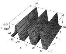
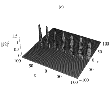
Figure 1: (a) Optical lattice for the choice $k(x)=(sin(0.1x)^{2}-4$ x $0.5)^{4}$ x $0.3$ with $A_{1}(t)=A_{2}(t)=1,{b_{0}(t)}={b_{1}(t)}=0$ and $\theta_{1}(t)=\theta_{2}(t)=1$ (b),(c) Grating solitons in the optical lattice potentials.

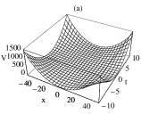
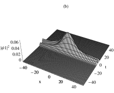
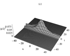
Figure 2: (a) Harmonic trap for the choice $k(x)=\frac{1}{0.9+cos(0.02x)^{2}}$ with $A_{1}(t)=A_{2}(t)=1,{b_{0}(t)}=0.1t,{b_{1}(t)}=-0.2t,\theta_{1}(t)=\theta_{2}(t)=sin(0.1t)$. (b),(c) Double hump matter wave solitons in the harmonic trap.

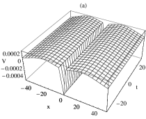
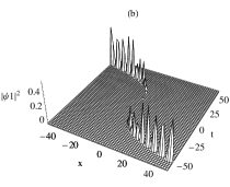
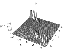
Figure 3: (a)Transient trap for the choice $k(x)=tanh(0.03x)^{2}+0.0001$ with $A_{1}(t)=A_{2}(t)=1$ and ${b_{0}(t)}={b_{1}(t)}=\theta_{1}(t)=\theta_{2}(t)=0$,(b)(c) Growth of matter wave solitons in the transient trap

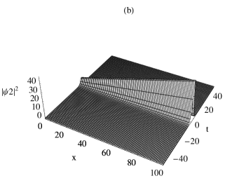
Figure 4: (a),(b)Matter wave solitons in the absence of the trap for $k(x)=(-x-4*5)^{4}$ x $0.3$

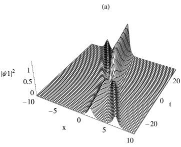
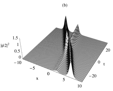
Figure 5: (a)(b)Switching of matter wave solitons for $k(x)=0.1cos(-0.3x)^{2}+0.1sin(-0.3x)^{2}$.

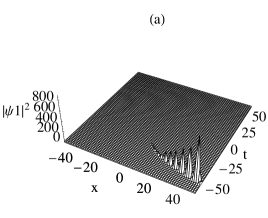
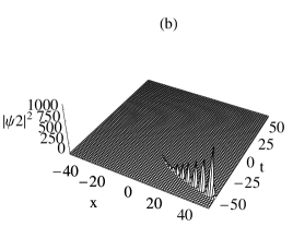
Figure 6: (a,b) Impact of spatio temporal interaction and abrupt increase of density of the condensates for $k(x)=tanh(0.03x)^{2}+0.0001$ with $A_{1}(t)=A_{2}(t)=e^{0.15t},{b_{0}(t)}={b_{1}(t)}=0$ and $\theta_{1}(t)=\theta_{2}(t)=1$

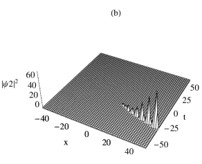
Figure 7: (a,b) Stabilization of the condensates by tuning spatial scattering length for $k(x)=tanh(0.03x)^{2}+0.0075$ with $A_{1}(t)=A_{2}(t)=e^{0.15t},{b_{0}(t)}={b_{1}(t)}=0$ and $\theta_{1}(t)=\theta_{2}(t)=1$

4.2 Matter wave solitons in harmonic traps

Selecting $k(x)=\frac{1}{0.9+cos(0.02x)^{2}}$ and again choosing the parameters $\theta_{1}(t),\theta_{2}(t),{b_{0}(t)}$ and ${b_{1}(t)}$ desirably, one obtains a harmonic trap as shown in figure (2a). Accordingly, one observes double hump solitons for the condensates $|\psi_{1}|^{2}$ and $|\psi_{2}|^{2}$ in figures (2b) and (2c) respectively. Again, the width and amplitude of the bright solitons can be altered by changing the parameters associated with $k(x)$. This underscores the fact that the energy associated with the modes $|\psi_{1}|^{2}$ and $|\psi_{2}|^{2}$ can be modulated desirably.

4.3 Transient trap behaviour

Choosing the transient trap as shown in fig (3a) (after appropriately choosing $k(x)$ and the parameters $\theta_{1}(t),\theta_{2}(t),{b_{0}(t)}$ and ${b_{1}(t)}$ suitably), the behaviour of the condensates in the transient trap is shown in figures (3b) and (3c). From the figures 3(a-c), one could observe the stabilization of the condensates in the confining trap while the life time of the expulsive domain is too short to notice the dynamics of the condensates.

4.4 Switching off the trap and bright soliton dynamics

Choosing the dispersion coefficient $k(x)=(-x-4$ x $5)^{4}$ x $0.3$, we observe that the external trap $V(x)$ becomes zero. Under this condition, we observe that the amplitude of the solitons keeps growing as they evolve in space and time as shown in figs (4a,b)and this increase of amplitude of matter wave solitons occurs without any addition of external energy for a specific choice of spatially inhomogeneous interaction.

   The gauge transformation approach can be easily extended to generate multisoliton solution [33] and the interaction of solitons can be analysed.

4.5 Matter wave switching

Choosing the spatially varying dispersion coefficient of the form $k(x)=0.1cos(-0.3x)^{2}+0.1sin(-0.3x)^{2}$, one observes switching of intensities of matter wave solitons as shown in the figs (5a,b). Thus, it is obvious from the figs (5 a,b) that the intensity redistribution occurs between the modes $|\psi_{1}|^{2}$ and $|\psi_{2}|^{2}$.

4.6 Impact of spatio temporal interaction on the condensates

It is obvious from the above that cases [(i)-(v)] discuss the effect of spatially inhomogeneous interaction alone on the condensates. To investigate the impact of spatiotemporal interaction on the condensates, we now consider the evolution of the condensates in the transient trap shown in figure (3a) corresponding to case (iii). Now, evolving the temporal scattering lengths of the form $A_{1}(t)=A_{2}(t)=e^{0.15t}$,the density of the condensates which were stabilized in the confining domain in the absence of temporal interaction now abruptly increases as shown in the figs (6a,b). We now suitably tune the spatially inhomogeneous interaction which subsequently reduces the density of the condensates. Hence, we observe that it should be possible to vary the spatially inhomogeneous interaction to stabilize the condensates just as one temporally varies the scattering length using Feshbach resonance as displayed in figs (7a,b) . It should be mentioned that this is the first instance of the occurrence of Feshbach resonance employing the variation of spatially inhomogeneous interaction. The combined effect of spatiotemporal interaction is that one can not only control the density of the condensates, but also design condensates with desirable density, shape (or geometry) and property leading to an era of ”designer quasi particle condensates”.

5 Discussion

In this paper, we have derived a new integrable model to investigate the dynamics of two component quasi-particle condensates with spatiotemporal interaction strengths and construct the associated Lax pair. We then generate the matter wave solitons and study their properties in harmonic and optical lattice potentials.

We also report the occurrence of Feshbach resonance by subtle variation of spatially inhomogeneous interaction. We reiterate that the simultaneous impact of spatio temporal interaction could possibly herald a new era of ”designer quasi particle condensates”.

6 Acknowledgements

PSV wishes to thank UGC and DAE-NBHM for financial support. The work of RR forms part of a research project sponsored by DST,DAE -NBHM and UGC. Authors thank the anonymous referee for his suggestions. RR wishes to thank Prof. Malomed for giving invaluable suggestions. KP acknowledges DST and CSIR, Government of India, for the financial support through major projects.

References

References

• [1] Anderson M H, Ensher J R, Matthews M R, Wieman C E and Cornell E A 1995 $Science$ 269 198
• [2] Davis K B, Mewes M O, Andrews M R, VanDruten N J, Durfee D S, Kurn D M and Ketterle W 1995 $Phys.Rev.Lett$ 75 3969
• [3] Dalfovo F, Giorgini S, Pitaevskii L P and Stringari S 1999 $Rev.Mod.Phys$ 71 463
• [4] Gross E P 1961 $Nuovo$ $Cimento$ 20 454
• [5] Gross E P 1963 $J.Math.Phys$ 4 195
• [6] Pitaevskii L P 1961 $Zh.Eksp.Teor.Fiz$ 40 646 $[$J. Exp. Theor. Phys 13 1961 451$]$
• [7] Liang Z X, Zhang Z D and Liu W M 2005 $Phys.Rev.Lett$ 94 050402
• [8] Radha R and Ramesh Kumar V 2007 $Phys.Lett.A$ 370 46
• [9] Radha R, Ramesh Kumar V and Porzeian K 2008 $J.Phys.A:Math.Theor$ 41 315209
• [10] Ramesh Kumar V, Radha R and Panigrahi P K 2008 $Phys.Rev.A$ 77 023611
• [11] Strecker K E, Partridge G B, Truscott A G and Hulet R G 2002 $Nature$ 417 150
• [12] Khaykovich L, Schreck F, Ferrari G, Bourdel T, Cubizolles J, Carr L D, Castin Y, Solomon C 2002 $Science$ 296 1290
• [13] Strecker K E, Partridge G B, Truscott A G and Hulet R G 2003 $New.J.Phys$ 5 73
• [14] Burger S, Bongs K, Dettmer S, Ertmer W, Sengstock K, Sanpera A, Shlyapnikov G V and Lewenstein M 1999 $Phys.Rev.Lett$ 83 5198
• [15] Denschlag J, Simsarian J E, Feder D L, Clark C W, Collins L A, Cubizolles J, Deng L, Hagley E W, Helmerson K, Reinhardt W P, Rolston S L, Schneider B I, Phillips W P 2000 $Science$ 287 5450.97.
• [16] Papp S B, Pino J M and Wieman C E 2008 $Phys.Rev.Lett$ 101 040402
• [17] Thalhammer G, Barontini G, Sarlo L De, Catani J, Minardi F and Inguscio M 2008 $Phys.Rev.Lett$ 100 210402
• [18] Nathan Kutz J 2009 $PhysicaD$ 238 1468
• [19] MiddelKamp S, Chang J J, Hamner C, Carretero-Gonzalez R, Kevrekidis P G, Achilleos V, Frantzeskakis D J, Schmelcher P, Engels P 2010 $Phys.Lett.A$ 375 642
• [20] Theocharis G, Schmelcher P, Kevrekidis P G, Frantzeskakis D J 2005 $Phys.Rev.A$ 72 033614
• [21] Rajendran S, Muruganandam P and Lakshmanan M 2009 $J.Phys.B.AtMol.Opt.Phys$ 42 145307
• [22] Ramesh Kumar V, Radha R and Wadati M 2010 $Phys.Lett.A$ 374 3685
• [23] Rodas-Verde M I, Michinel H and Perez-Garcia V M 2005 $Phys.Rev.Lett$ 95 153903
• [24] Carpentier A V, Michinel H, Rodas-Verde M I and Perez-Garcia V M 2006 $Phys.Rev.A$ 74 013619
• [25] Shin H J, Radha R, Ramesh Kumar V 2011 $Phys.Lett.A$ 375 2519
• [26] He J S, Mei J and Li Y S 2007 $Chin.Phys.Lett.$ 24 2157
• [27] He J S and Li Y S 2011 $Stud.Appl.Math.$ 126 1
• [28] Wang Y Y, He J S and Li Y S 2011 $Commun.Theor.Phys.$ 56 995
• [29] Xu S W, He J S and Wang L H 2012 $Europhys.Lett.$ 97 30007
• [30] He X G, Zhao D, Li L and Luo H G 2009 $Phys.Rev.E$ 79 056610
• [31] Wen L, Li L, Li Z D, Song S W, Zhang X F and Liu W M 2011 $Eur.Phys.J.D$ 64 473
• [32] Manakov S V 1974 $Sov.Phys.JETP.$ 38 248
• [33] Chau L L, Shaw J C and Yen H C 1991 $J.Math.Phys$ 32 1737
• [34] lizuka T, Wadati M 1997 $J.Phys.Soc.Jpn$ 66 2308