Transitional $\gamma$ strength in Cd isotopes

Abstract

The level densities and $\gamma$-ray strength functions of ^{105,106,111,112}Cd have been extracted from particle-$\gamma$ coincidence data using the Oslo method. The level densities are in very good agreement with known levels at low excitation energy. The $\gamma$-ray strength functions display no strong enhancement for low $\gamma$ energies. However, more low-energy strength is apparent for ^105,106Cd than for ^111,112Cd. For $\gamma$ energies above $\approx$ 4 MeV, there is evidence for some extra strength, similar to what has been previously observed for the Sn isotopes. The origin of this extra strength is unclear; it might be due to $E1$ and $M1$ transitions originating from neutron skin oscillations or the spin-flip resonance, respectively.

I Introduction

Recent measurements on the $\gamma$-strength function of several nuclei in the Fe-Mo mass region have revealed an unexpected enhancement for low $\gamma$ energies ($E_{\gamma}\leq 3-4$ MeV) Fe_Alex ; Mo_RSF ; V ; Sc ; magne_46Ti . However, no such feature was seen in the heavier Sn isotopes Sn_RSF ; Heidi_Sn2 or in the rare-earth region undraa ; bagheri ; hildes_DyRSF .

For ⁹⁵Mo, this low-energy enhancement has very recently been confirmed by an independent measurement and method wiedeking95Mo . It has also been shown in Ref. larsen_goriely , that if this increase persists in exotic nuclei close to the neutron drip line, it could boost the Maxwellian-averaged neutron-capture cross sections up to two orders of magnitude.

However, as of today, there are more questions than answers regarding the low-energy enhancement. There is no theoretical work predicting such a behavior, the underlying physics is unknown, neither the multipolarity nor the electromagnetic character have been determined, and nobody knows for which nuclei the onset of this structure takes place.

So far, there is only one nucleus, ⁶⁰Ni, where there are strong indications that the enhancement is due to $M1$ transitions Ni_Alex . One should however be careful to draw any general conclusions, because ⁶⁰Ni is in many ways a special case. It has only positive-parity states below excitation energies of $\approx 4.5$ MeV, which has significant consequences for the two-step cascade method employed in Ref. Ni_Alex . As discussed in Ref. Ni_Alex , it means that for the secondary $\gamma$ ray, $M1$ transitions are strongly enhanced compared to $E1$ transitions.

The motivation for this work is to determine the transitional region of the low-energy enhancement by investigating the $\gamma$-strength function of Cd isotopes using the Oslo method. The Cd isotopes have $Z=48$ and are in between Sn ($Z=50$) and Mo ($Z=42$). Thus, these experiments are a part of the experimental campaign exploring the onset of the low-energy enhancement.

In Sec. II, we give the experimental details and briefly describe the data analysis. In Sec. III, the normalization procedure of the level densities and $\gamma$-strength functions is discussed. Further, we compare the measured $\gamma$-strength functions with semi-empirical models in Sec. IV. Finally, we give a summary and outlook in Sec. V.

II Experimental details and data analysis

The experiments were performed at the Oslo Cyclotron Laboratory (OCL), utilizing a 38-MeV ³He beam delivered by the Scanditronix cyclotron. In the first experiment, the beam was bombarding a self-supporting target of ¹⁰⁶Cd (96.7% enrichment) with mass thickness 1.1 mg/cm². Typical beam currents were $0.3-0.5$ electrical nA (charge state ³He²⁺). In the second experiment, the target was 99.5% ¹¹²Cd with mass thickness $0.95$ mg/cm². The beam current was $\approx 0.1-0.2$ electrical nA (charge state ³He²⁺). Both experiments were run for five days. The reactions of interest are ^106,112Cd(³He,³He^′$\gamma$)^106,112Cd and ^106,112Cd(³He,$\alpha\gamma$)^105,111Cd. The $Q$-values of the pick-up reactions are $9703.9(124)$ keV and $11183.295(3)$ keV, respectively qcalc .

Particle-$\gamma$ coincidences were measured with the Silicon Ring (SiRi) particle-detector system siri and the CACTUS array for detecting $\gamma$ rays CACTUS . The SiRi system consists of eight 130-$\mu$m thick silicon detectors, where each of them is divided into eight strips. One strip has an angular resolution of $\Delta\theta=2^{\circ}$. Each of these segmented, thin detectors are put in front of a 1550-$\mu$m thick back detector. The full SiRi system has then 64 individual detectors in total, covering scattering angles between $40-54^{\circ}$ and a solid-angle coverage of $\approx 6$%. For the Cd experiments, SiRi was placed in forward angles with respect to the beam direction.

The CACTUS array consists of 28 collimated $5"\times 5"$ NaI(Tl) crystals. The total efficiency of CACTUS is $15.2(1)$% at $E_{\gamma}=1332.5$ keV. The charged ejectiles and the $\gamma$-rays were measured in coincidence event-by-event, with time resolution of $\approx 15$ ns.

Using the $\Delta E-E$ technique, each charged-particle species was identified. Gates were set on the ³He and $\alpha$ ejectiles to select the correct reaction channel. Furthermore, the reaction kinematics and the known $Q$-value for the reaction allowed us to relate the measured ejectile energy to the excitation energy of the residual nucleus.

In Fig. 1, the ³He and $\alpha$ spectra with and without $\gamma$-coincidence requirements are shown.

Figure 1: (Color online) Singles particle spectra (blue) and in coincidence with $\gamma$ rays (red) from (a) the ¹¹²Cd(³He,$\alpha)$ reaction and (b) the ¹¹²Cd(³He,³He^′) reaction. The dashed lines indicate the neutron separation energies for the final nucleus.

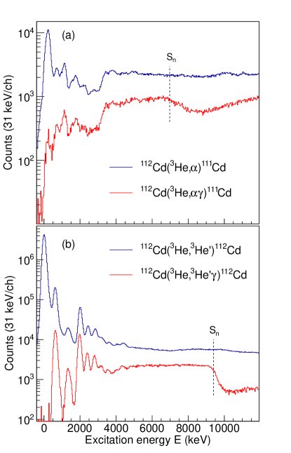
It is interesting to see how the ³He and $\alpha$ spectra in coincidence with $\gamma$ rays differ at the neutron separation energy. They both display a drop because the neutron channel is open. However, while the ³He spectrum shows a rather abrupt drop (compatible with the energy resolution of $\approx 200$ keV), the slope of the $\alpha$ spectrum is much less steep and a minimum is not reached until $\approx S_{n}+1.5$ MeV. This can be explained by considering the final nuclei in the reactions ¹¹²Cd(³He,³He^′$n\gamma$)¹¹¹Cd and ¹¹²Cd(³He,$\alpha n\gamma$)¹¹⁰Cd. In the latter case, the odd, final nucleus ¹¹¹Cd has many states within a relatively broad spin window at low excitation energy. However, this is not so for ¹¹⁰Cd, where there are only $0^{+}$ and $2^{+}$ states below $\approx 1.5$ MeV. As the (³He,$\alpha$) reaction favors high-$\ell$ transfer in general, the populated states very likely have an average spin larger than $2$. Thus, there is an effective spin hindrance which explains the observed behavior in the $\alpha$ spectrum.

The $\gamma$-ray spectra for each excitation-energy bin were unfolded using the known response functions of the CACTUS array, as described in Ref. gutt6 . The main advantage of this method is that the experimental statistical uncertainties are preserved, without introducing new, artificial fluctuations.

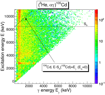
The matrix of unfolded $\gamma$ spectra for each excitation-energy bin is shown for ¹⁰⁵Cd in Fig. 2. One may notice a peculiar feature in this matrix. Surprisingly, there is a considerable amount of $\gamma$ rays from ¹⁰⁵Cd that survive several MeV above $S_{n}$, see the region to the right of the dashed-dotted line in Fig. 2. For example, the intensity of 5-MeV $\gamma$ rays is practically the same for the excitation-energy region $7.0-8.0$ MeV and $8.5-9.5$ MeV. This could be caused by the difference in spin between the populated initial states and the spin of the first excited states in ¹⁰⁴Cd ($2^{+},4^{+}$).

Figure 2: (Color online) Excitation energy vs. $\gamma$ energy matrix for ¹⁰⁵Cd. The $\gamma$-ray spectra are unfolded for each excitation-energy bin. The dashed line indicates the neutron separation energy in ¹⁰⁵Cd. The dashed-dotted line shows where the $E=E_{\gamma}$ diagonal would be in ¹⁰⁴Cd for the extreme case where the outgoing neutron has zero kinetic energy.

After the $\gamma$ spectra were unfolded, the distribution of first-generation $\gamma$ rays for each excitation-energy bin was extracted via an iterative subtraction technique Gut87 . The basic assumption of this method is that the decay routes are the same regardless of the population mechanism of the initial states (either directly via the nuclear reaction or from $\gamma$ decay from above-lying states). For a discussion of uncertainties and possible errors of the first-generation method, see Ref. systematic .

From the excitation energy vs. first-generation $\gamma$-ray matrix, one can extract the functional form of the level density and the $\gamma$ transmission coefficient. This is done with an iterative procedure as described in Ref. Schiller00 , with the following ansatz:

$$P(E,E_{\gamma})\propto\rho(E_{\mathrm{f}}){\mathcal{T}}(E_{\gamma}).$$ (1)

Here, $P(E,E_{\gamma})$ is the experimental first-generation matrix, $\rho(E_{\mathrm{f}})$ is the level density at the final excitation energy $E_{\mathrm{f}}$, with $E_{\mathrm{f}}=E-E_{\gamma}$, and ${\mathcal{T}}(E_{\gamma})$ is the $\gamma$-transmission coefficient. Every point of the $\rho$ and ${\mathcal{T}}$ functions is assumed to be an independent variable, and a global $\chi^{2}$ minimum is reached typically within 10–20 iterations.

The method is based on the assumption that the reaction leaves the product nucleus in a compound state, which then subsequently decays in a manner that is independent on the way it was formed, i.e. a statistical decay process BM . Therefore, a lower limit is set in the excitation energy to ensure that decay from compound states dominates the spectra. In addition, an upper excitation-energy limit at $\approx S_{n}$ is employed. Because of methodical problems with the first-generation method for low $\gamma$ energies, $\gamma$ rays below $\approx 1.0$ and $1.5$ MeV for ^105,111Cd and ^106,112Cd, respectively, were excluded from the further analysis (see also Ref. systematic ).

The $\gamma$-transmission coefficient ${\cal T}$ is a function of $E_{\gamma}$ only, in accordance with the Brink hypothesis brink , which in its generalized form states that any collective decay mode has the same properties whether it is built on the ground state or on excited states. This assumption is proven to be incorrect for nuclear reactions involving high temperatures and/or spins, see for example Ref. Andreas&Thoennessen . However, in the present work, neither high-spin states nor high temperatures are reached ($T_{\mathrm{f}}\propto\sqrt{E_{\mathrm{f}}}$, and the populated spin range is centered within $J\sim 2-8\hbar$). Therefore, eventual spin and/or temperature dependencies should not have a significant impact on the results.

III Normalization of level density and $\gamma$-strength function

The extracted level density and the $\gamma$-ray transmission coefficient give identical fits to the experimental data with the transformations Schiller00

$$\tilde{\rho}(E-E_{\gamma}) = {\mathcal{A}}\exp[\alpha(E-E_{\gamma})]\,\rho(E-E_{\gamma}),$$ (2)

$$\tilde{{\mathcal{T}}}(E_{\gamma}) = {\mathcal{B}}\exp(\alpha E_{\gamma}){\mathcal{T}}(E_{\gamma}).$$ (3)

Therefore, the transformation parameters ${\mathcal{A}}$, $\alpha$, and ${\mathcal{B}}$ were determined from external data.

III.1 Level density

For the level density, the absolute normalization ${\mathcal{A}}$ and the slope $\alpha$ can be determined from the known, discrete levels ENSDF at low excitation energy, and from neutron-resonance spacings at the neutron separation energy $S_{n}$ RIPL . For the latter, we must estimate the total level density at $S_{n}$ from the neutron resonances, which are for a few spins only. Also, because of the selected lower limit of $E_{\gamma}$ for the extraction of $\rho$ and ${\mathcal{T}}$ (see Sec. II), our level-density data reach up to $E\approx S_{n}-1$ MeV. Therefore, we must interpolate between our data and the level density at $S_{n}$. We have here chosen to use the back-shifted Fermi gas (FG) model with the parameterization of von Egidy and Bucurescu egidy2 for that purpose.

Because the spin distribution is poorly known at high excitation energies, a systematic uncertainty will be introduced to the slope of the level density and $\gamma$-strength function (see Ref. systematic for a thorough discussion on this subject). In addition, the light-ion reactions in the experiments populate only a certain spin range, which usually is for rather low spins. Therefore, the full spin distribution should also be folded with the experimental spin distribution.

In this work, we have tested two different approaches to normalize the level densities. First, we have used the back-shifted Fermi gas parameterization of von Egidy and Bucurescu egidy2 to estimate the total level density at the neutron separation energy, $\rho(S_{n})$. Second, we have used the microscopic level densities of Goriely, Hilaire and Koning go08 at high excitation energies. These level densities are calculated within the combinatorial plus Hartree-Fock-Bogoliubov approach, and are resolved in spin and parity. The applied parameters are listed in Tab. 1, together with the Fermi-gas parameters of Ref. egidy2 used for the interpolation between our data and the estimated $\rho(S_{n})$.

We start with the back-shifted Fermi gas approach. We adopt the expression for the spin cutoff parameter from Ref. egidy2 :

$$\sigma^{2}(E)=0.0146A^{5/3}\frac{1+\sqrt{1+4a(E-E_{1})}}{2a},$$ (4)

where $A$ is the mass number, $a$ is the level density parameter and $E_{1}$ is the backshift parameter (see Ref. egidy2 for further details). The total level density can be calculated by

$$\rho(S_{n})=\frac{2\sigma^{2}}{D_{0}}\cdot\frac{1}{(I_{t}+1)\exp\left[-(I_{t}+1)^{2}/2\sigma^{2}\right]+I_{t}\exp\left[-I_{t}^{2}/2\sigma^{2}\right]},$$ (5)

where $D_{0}$ is the level spacing of $s$-wave neutrons and $I_{t}$ is the ground-state spin of the target nucleus in the $(n,\gamma)$ reaction. In Eq. (5), it is assumed that both parities contribute equally to the level density at $S_{n}$ (see Refs. Schiller00 and systematic ).

From the Fermi-gas calculation, we get $\rho_{\mathrm{FG}}(S_{n})$, which differs somewhat from the semi-experimental value $\rho(S_{n})$. Therefore, a correction factor $\eta$ is applied to ensure that the Fermi-gas interpolation matches $\rho(S_{n})$ (see Tab. 1).

Table 1: Parameters used for the calculation of $\rho(S_{n})$ (see text).

Nucleus	$I_{t}^{\pi}$	$D_{0}$	$S_{n}$	$\sigma(S_{n})$	$a$	$E_{1}$	$\rho_{\mathrm{FG}}(S_{n})$	$\rho(S_{n})$	$\eta$	$\tilde{\sigma}(S_{n})$	$\tilde{\rho}(S_{n})$	shift $E_{\mathrm{HFB}}$	range $I_{i}$
		(eV)	(MeV)		(MeV-1)	(MeV)	($10^{5}$ MeV-1)	($10^{5}$ MeV-1)			($10^{5}$ MeV-1)	(MeV)	($\hbar$)
105Cd	$0^{+}$	$-$	8.427	5.71	10.88	-0.567	1.43	1.78(89)a	1.25	4.5	1.11(56)a	0.042	$1/2-13/2$
106Cd	$5/2^{+}$	$-$	10.874	5.85	11.39	0.746	6.44	8.05(40)a	1.25	4.5	5.3(26)a	0.052	$0-6$
111Cd	$0^{+}$	155(20)	6.976	5.43	13.56	-0.640	2.99	3.87(91)	1.29	4.5	2.68(72)	0.435	$1/2-13/2$
112Cd	$1/2^{+}$	27(2)	9.394	5.61	13.82	0.713	11.9	12.0(25)	1.01	4.5	7.8(16)	0.540	$0-6$

^a Estimated from systematics.

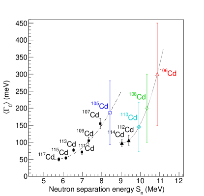
As there is no information on the level spacing for ^105,106Cd (^104,105Cd are unstable), we have estimated the total level density at the neutron separation energy from systematics for these nuclei, see Fig. 3. Here, we have calculated the semi-experimental $\rho(S_{n})$ for all Cd isotopes where the neutron resonance spacing $D_{0}$ is known. For all $D_{0}$ values we have used the Reference Input Parameter Library (RIPL-3) evaluation RIPL , except for ¹¹⁷Cd where we have also used the RIPL-2 value.

Figure 3: (Color online) Estimation of $\rho(S_{n})$ for ^105,106Cd. The filled, black squares are calculated from known neutron resonance spacings in RIPL-3 RIPL using Eq. (5) with $\sigma$ values from Ref. egidy2 . The filled, violet square is the result for ¹¹⁷Cd using the $D_{0}$ value recommended in RIPL-2. The small, open diamonds connected with lines are calculated values from the back-shifted Fermi gas approach egidy2 multiplied with a common factor of 1.25 to bring them within the error bars of the semi-experimental $\rho(S_{n})$ values. The blue, open square and the red, open cross are the estimated values for $\rho(S_{n})$ of ^105,106Cd, respectively.

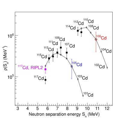
It is striking how the values of $\rho(S_{n})$ actually decrease as a function of $S_{n}$ for the isotopes with $A\leq 108$. This is probably an effect of approaching the $N=50$ closed shell. It is, however, unfortunate that there are no experimental $D_{0}$ values for these nuclei, so the uncertainty of the estimated $\rho(S_{n})$ for ^105,106Cd must necessarily be large; we have assumed a 50% uncertainty.

The normalization procedure is demonstrated for ¹¹²Cd in Fig. 4.

Figure 4: Normalization of the level density of ¹¹²Cd to the known, discrete levels (jagged line), and $\rho(S_{n})$ (see text).

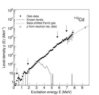
The agreement between our data and the discrete levels ENSDF is very satisfying. We notice however that the ground state seems to be underestimated; this is probably because there are very few direct decays to the ground state, most of the decay goes through the first $2^{+}$ state. We also see that the triplet of two-phonon vibrational states $0^{+}$, $2^{+}$, $4^{+}$, at about $E\approx 1.4$ MeV, is clearly seen in our level-density data, as well as the one-phonon first excited $2^{+}$ state at $0.62$ MeV (see, e.g., Ref. garrett for a discussion on the vibrational nature of Cd isotopes).

The level densities normalized with the back-shifted Fermi gas approach are shown in Fig. 5a.

Figure 5: (Color online) Normalized level densities of ^{105,106,111,112}Cd with (a) the fermi-gas approach and (b) the combinatorial plus Hartree-Fock-Bogoliubov approach.

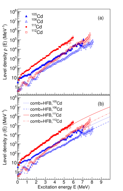
Again, the effect of approaching the $N=50$ closed shell is clearly seen. The slope in level density is smaller for ^105,106Cd than for ^111,112Cd. Also, we see that the level densities of the neighboring isotopes are parallel, but the increase in level density of the odd-$A$ nucleus compared to the even neighbor is smaller for ¹⁰⁵Cd than for ¹¹¹Cd.

For the second approach, we have used the combinatorial plus HFB calculations of Ref. go08 . Here, we have normalized our data to obtain a best fit to the microscopic level densities at high excitation energies ($E\geq 4-5$ MeV). As described in Ref. go08 , an energy shift is used in order to optimize the reproduction of the known, discrete levels. The applied energy shifts are listed in Tab. 1.

The level-density data normalized to the microscopic calculations are shown in Fig. 5b. It is seen that the two independent normalization methods yield very similar results.

We have also taken into account that the spin distribution of the initial levels could be rather narrow. As discussed in Ref. guttormsen_spin , the (³He,$\alpha$) reaction in forward angles gives an average spin transfer of $\approx 5\hbar$ at $E\approx 5$ MeV in the rare-earth region. For excitation energies below 3 MeV, it is shown in Ref. dracoulis that the ¹⁰⁶Cd(³He,$\alpha$)¹⁰⁵Cd reaction involves $\ell=2,4,$ and 5.

Turning to the inelastic scattering, where vibrational states are favored, we see from the ^106,112Cd data below $E\approx 3$ MeV that levels with $I=2,3,4$ are strongly populated. For levels with higher spins the data are inconclusive, but it is clear that they are significantly less populated. We therefore estimate a reduced spin cutoff parameter, $\tilde{\sigma}$, to be $\approx 4.5$ for all the Cd nuclei studied here. This corresponds to a reduced level density at $S_{n}$, $\tilde{\rho}(S_{n})$. For the microscopic level densities, which are spin-dependent, we filter out the levels within the approximate experimental spin range (see Tab. 1).

The four different normalizations are shown for ¹¹²Cd for $E=3-8$ MeV in Fig. 6.

Figure 6: (Color online) The various normalizations of ¹¹²Cd: the fermi-gas approach (FG, red squares), FG approach with a reduced spin-cutoff parameter (red, open squares), the combinatorial plus HFB approach (blue triangles) and with a reduced spin range (open, blue triangles).

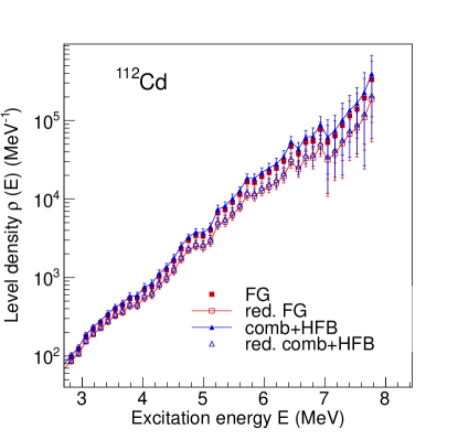
As seen in this figure, the effect of the reduced spin range is not large at low excitation energies, but could be as much as a factor of 2 for example at $E=7.9$ MeV.

III.2 Gamma strength function

The slope of the $\gamma$ strength function is given by the slope of the level density, see Eqs. (2) and (3). Therefore, the only parameter left to determine is the absolute value $\mathcal{B}$. This is done using known values on the average, total radiative width at $S_{n}$, $\left<\Gamma_{\gamma 0}\right>$, extracted from $s$-wave neutron resonances RIPL by voin1 :

$$\langle\Gamma_{\gamma}(S_{n},I_{t}\pm 1/2, \pi_{t})\rangle=\frac{D_{0}}{4\pi}\int_{E_{\gamma}=0}^{S_{n}}\mathrm{d}E_{\gamma}{\mathcal{B}}\mathcal{T}(E_{\gamma})$$

$$\times\rho(S_{n}-E_{\gamma})\sum_{I=-1}^{1}g(S_{n}-E_{\gamma},I_{t}\pm 1/2+I),$$ (6)

where $I_{t}$ and $\pi_{t}$ are the spin and parity of the target nucleus in the $(n,\gamma)$ reaction, and $\rho(S_{n}-E_{\gamma})$ is the experimental level density. The spin distribution is assumed to be given by GC :

$$g(E,I)\simeq\frac{2I+1}{2\sigma^{2}}\exp\left[-(I+1/2)^{2}/2\sigma^{2}\right]$$ (7)

for a specific excitation energy $E$, spin $I$, and a spin cutoff parameter $\sigma$. All values are known in Eq. (6) except the parameter $\mathcal{B}$, which can now be determined.

For ^111,112Cd, the values for $\left<\Gamma_{\gamma 0}\right>$ are 71(6) and 106(15) meV, respectively. However, again we lack neutron resonance data for ^105,106Cd. We must therefore estimate $\left<\Gamma_{\gamma 0}\right>$ and $D_{0}$ for these nuclei. For the FG approach, $D_{0}$ is evaluated from the previously estimated $\rho(S_{n})$ values (see Tab. 1). We get $D_{0}=375(188)$ and 16.3(82) eV for ^105,106Cd, respectively. The combinatorial plus HFB calculations predict $D_{0}=294$ eV and 13.6 eV for ^105,106Cd, respectively.

Figure 7: (Color online) Estimation of $\left<\Gamma_{\gamma 0}\right>$ for ^105,106Cd (see text). The black squares are known values for odd Cd isotopes and the black triangles are for the even ones; all values are taken from Ref. RIPL . The dashed-dotted line represents the best fit with a quadratic function for the odd nuclei. The blue, open square is the estimated $\left<\Gamma_{\gamma}\right>$ for ¹⁰⁵Cd, and the red, open triangle for ¹⁰⁶Cd. The dashed line indicates a quadratic function for the even isotopes in the same fashion as for the odd ones. Estimations of ^108,110Cd are shown for completeness (green, open diamond and cyan, open cross, respectively).

To estimate the average total radiative width, we have considered systematics from the Cd isotopes where $\left<\Gamma_{\gamma 0}\right>$ is known, see Fig. 7. It is difficult to predict with reasonable certainty the unknown values for ^105,106Cd because of the possible shell effects. Because we also lack data on ^108,110Cd, it is especially problematic for ¹⁰⁶Cd. We have therefore also assumed that for $\gamma$ energies above $\approx 5-6$ MeV, the strength functions for all the Cd isotopes should be very similar, because this region should be dominated by the low-energy tail of the Giant Electric Dipole Resonance (GDR). The GDR is mainly governed by the number of protons, and thus it is reasonable to believe that the properties should be the same for all Cd isotopes, at least to a large extent.

As shown in Fig. 7, we have fitted a quadratic function to the $\left<\Gamma_{\gamma 0}\right>$ values of the odd Cd isotopes, and for ¹⁰⁵Cd we estimate $\left<\Gamma_{\gamma 0}\right>=187(94)$ meV. For the even isotopes, we only have two data points. However, considering the trend for the odd isotopes and claiming the postulated similarity of the strength functions at high $E_{\gamma}$, we have chosen a rather large value of 300(150) meV. To guide the eye, we have shown a quadratic fit as for the odd case, and displayed the predicted $\left<\Gamma_{\gamma 0}\right>$ values also for ^108,110Cd (see Fig. 7).

The normalized $\gamma$ strength functions for the four different level-density normalizations of ^{105,106,111,112}Cd are shown in Fig. 8.

Figure 8: (Color online) Gamma-ray strength functions of (a) ¹⁰⁵Cd, (b) ¹⁰⁶Cd, (c) ¹¹¹Cd, and (d) ¹¹²Cd for the four different normalization approaches on the level densities.

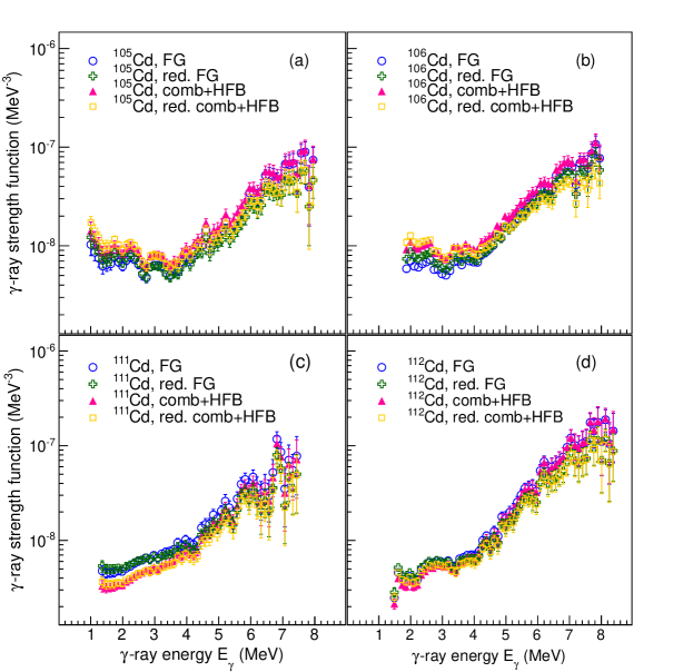
We clearly see a difference in the strength for $E_{\gamma}<4$ MeV for the heavier ^111,112Cd compared to the lighter ^105,106Cd. For the latter, the tendency is a more flat and even a slightly increasing $\gamma$-strength function, while for the former the $\gamma$ strength is decreasing when $E_{\gamma}$ decreases. Although there is no strong low-energy enhancement as in Fe or Mo, it could indicate that this is the transitional mass region for the low-energy enhancement of the $\gamma$ strength.

Another observation is that all the Cd strength functions seem to change slope at $E_{\gamma}\approx 4$ MeV. Above this value, the slope is significantly steeper than for lower $\gamma$ energies. This has previously been seen in Sn isotopes Sn_RSF ; Heidi_Sn2 . These issues will be further addressed in the following section.

IV Comparison with other data and models

As mentioned in the previous section, our Cd data on the $\gamma$-strength function lack a strong low-energy enhancement, although the lighter isotopes appear to have more low-energy strength than the heavier ones. In addition, it is very likely that some extra strength is present in the region of $4\leq E_{\gamma}\leq 8$ MeV.

Figure 9: (Color online) Comparison of $\gamma$ strength functions of ⁹⁵Mo, ^105,112Cd, and ¹¹⁷Sn (see text).

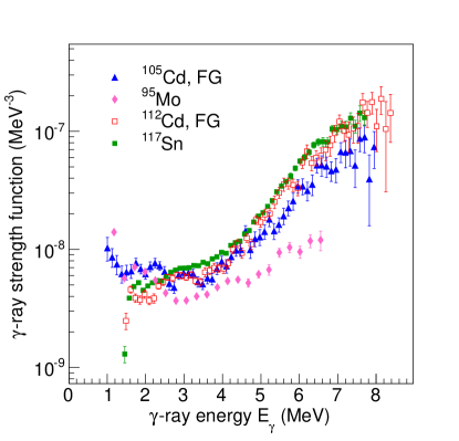
In Fig. 9, we have compared the strength functions of ^105,112Cd with ⁹⁵Mo Mo_RSF and ¹¹⁷Sn Sn_RSF . It is very interesting to see how much ¹¹²Cd resembles ¹¹⁷Sn. On the other hand, ⁹⁵Mo is very different from both ¹¹²Cd and ¹¹⁷Sn, while ¹⁰⁵Cd seems to be somewhat in between ⁹⁵Mo and ¹¹⁷Sn for $2\leq E_{\gamma}\leq 4$ MeV. For higher $\gamma$ energies, also ¹⁰⁵Cd looks very much the same as ¹¹⁷Sn.

To gain more insight of the observed $\gamma$ strength functions, we would like to compare our data with model calculations. One of the more widely used models for the $E1$ $\gamma$ strength is the Generalized Lorentzian (GLO) model ko87 ; ko90 . This is a model tailored to give a reasonable description both on the photoabsorption cross section in the GDR region, and on the $\gamma$ strength below the neutron separation energy. It is in principle dependent on the temperature of the final states $T_{f}$, which is in contradiction to the Brink hypothesis brink . However, by introducing a constant temperature, the hypothesis is regained.

The strength function within the GLO model is given by

$$f_{\rm GLO}(E_{\gamma},T_{f})=\frac{1}{3\pi^{2}\hbar^{2}c^{2}}\sigma_{E1}\Gamma_{E1}\times$$ (8)

$$\left[\frac{E_{\gamma}\Gamma(E_{\gamma},T_{f})}{(E_{\gamma}^{2}-E_{E1}^{2})^{2}+E_{\gamma}^{2}\Gamma(E_{\gamma},T_{f})^{2}}+\;0.7\frac{\Gamma(E_{\gamma}=0,T_{f})}{E_{E1}^{3}}\right],$$

with

$$\Gamma(E_{\gamma},T_{f})=\frac{\Gamma_{E1}}{E_{E1}^{2}}(E_{\gamma}^{2}+4\pi^{2}T_{f}^{2}).$$ (9)

The Lorentzian parameters $\Gamma_{E1}$, $E_{E1}$ and $\sigma_{E1}$ correspond to the width, centroid energy, and peak cross section of the GDR. We have made use of the parameterization of RIPL-2 RIPL to estimate the GDR parameters as these are unknown experimentally for the individual Cd isotopes, see Tab. 2. Because the even-even Cd isotopes are known to have a non-zero ground-state deformation RIPL , the GDR is split in two and we have therefore two sets of Lorentzian parameters (denoted by subscripts 1 and 2, see Tab. 2).

Table 2: Parameters used for the RSF models.

Nucleus	$E_{E1,1}$	$\sigma_{E1,1}$	$\Gamma_{E1,1}$	$E_{E1,2}$	$\sigma_{E1,2}$	$\Gamma_{E1,2}$	$T_{\mathrm{min}}$	$T_{\mathrm{max}}$	$E_{M1}$	$\sigma_{M1}$	$\Gamma_{M1}$	$E_{\mathrm{pyg}}$	$\sigma_{\mathrm{pyg}}$	$C_{\mathrm{pyg}}(T_{\mathrm{min}})$	$C_{\mathrm{pyg}}(T_{\mathrm{max}})$
	(MeV)	(mb)	(MeV)	(MeV)	(mb)	(MeV)	(MeV)	(MeV)	(MeV)	(mb)	(MeV)	(MeV)	(MeV)	($10^{-7}$ MeV-2)	($10^{-7}$ MeV-2)
105Cd	14.7	151.8	4.39	17.0	75.8	5.81	0.35	0.40	8.69	0.94	4.0	8.7(2)	1.5(1)	2.2(2)	1.1(1)
106Cd	14.6	153.7	4.37	16.9	76.7	5.79	0.35	0.40	8.66	0.94	4.0	8.7(2)	1.5(1)	2.4(2)	1.1(2)
111Cd	14.5	162.8	4.28	16.8	81.3	5.67	0.37	0.47	8.53	0.90	4.0	8.7(2)	1.5(1)	2.9(3)	1.7(2)
112Cd	14.4	164.5	4.26	16.7	82.1	5.65	0.37	0.40	8.51	0.89	4.0	8.7(2)	1.5(1)	3.7(3)	2.4(4)

For the $M1$ strength, we have used a Lorentzian shape with the parameterization in Ref. RIPL .

We treat the extra strength for high $\gamma$ energies in the same way as for the Sn isotopes Sn_RSF ; Heidi_Sn2 , adding a Gaussian-shaped pygmy resonance:

$$f_{\mathrm{pyg}}=C_{\mathrm{pyg}}\cdot\frac{1}{\sqrt{2\pi}\sigma_{\mathrm{pyg}}}\exp\left[\frac{-(E_{\gamma}-E_{\mathrm{pyg}})^{2}}{2\sigma_{\mathrm{pyg}}^{2}}\right].$$ (10)

Here, $C_{\mathrm{pyg}}$ is a normalization constant, $\sigma_{\mathrm{pyg}}$ is the standard deviation, and $E_{\mathrm{pyg}}$ is the centroid of the resonance.

The temperature of the final states is assumed to be constant, and is treated as a free parameter to get the best possible agreement with our data. As the normalization is uncertain, also the temperature is uncertain. In general, we get a slightly higher temperature for the normalization options that give the largest low-energy $\gamma$ strength. We denote the temperature for the normalization giving the largest low-energy strength $T_{\mathrm{max}}$, and the smallest low-energy strength $T_{\mathrm{min}}$. The adopted $\gamma$-strength model parameters are given in Tab. 2.

As there are no photoneutron cross-section data on the individual Cd isotopes, we have compared our measurements with $(\gamma,x)$ data on natural Cd from Ref. lepretreCd and ($\gamma,n$) data on ^106,108Pd taken from Ref. hiro106Pd . Assuming that the photoneutron cross section $\sigma_{\gamma}(E_{\gamma})$ is dominated by dipole transitions, we convert it into $\gamma$ strength by RIPL :

$$f_{\gamma}(E_{\gamma})=\frac{1}{3\pi^{2}\hbar^{2}c^{2}}\frac{\sigma_{\gamma}}{E_{\gamma}}.$$ (11)

In Fig. 10, our data on the $\gamma$ strength function of ¹⁰⁵Cd and the photonuclear data are shown together with the model calculations for the lowest temperature $T_{\mathrm{min}}$ in the GLO model.

Figure 10: (Color online) Calculations using the GLO model with a constant temperature ($T_{\mathrm{min}}$) and a variable temperature ($T_{f}\propto\sqrt{E_{f}}$) compared to data of ¹⁰⁵Cd for the normalization giving the lowest possible low-energy strength (FG) and the highest (combinatorial-plus-HFB, reduced spin window). The black triangles show the extracted strength function for a higher cut on $E_{\gamma}$ and $E$ in the first-generation matrix of ¹⁰⁵Cd. Photonuclear data from Refs. lepretreCd ; hiro106Pd are also shown.

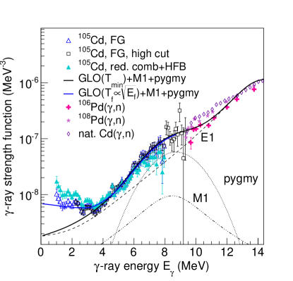
It can be seen that the calculations are in reasonable agreement with the Pd data from Ref. hiro106Pd and our data down to $E_{\gamma}\approx 3.5$ MeV. For lower $\gamma$ energies, our data show significantly more strength than the constant-temperature calculations.

Because $\gamma$ decay has a considerable probability also above $S_{n}$ for ¹⁰⁵Cd, see Fig. 2, we have extracted the strength function for this nucleus up to $E_{\gamma}\approx 9.3$ MeV. This is done by choosing a higher $E_{\gamma}$ limit of 2.25 MeV in the first-generation matrix to ensure that we do not mix with data from the ¹⁰⁴Cd channel. The resulting strength function is displayed in Fig. 10 as open squares. Although the statistical errors are quite large, we are able to bridge the gap up to the $(\gamma,n)$ measurements, thus further supporting the presence of an enhanced strength in the $6-10$ MeV region. It is also a strong indication that the $\left<\Gamma_{\gamma}\right>$ value we have chosen for normalization is reasonable.

The resulting $\gamma$-strength models for all the Cd isotopes studied here are shown together with our data and the photonuclear data in Fig. 11.

Figure 11: (Color online) Modeled $\gamma$ strength functions compared to the data for (a) ¹⁰⁵Cd, (b) ¹⁰⁶Cd, (c) ¹¹¹Cd, and (d) ¹¹²Cd for the level-density normalizations which give the minimum or maximum strength at low $\gamma$ energies. Photonuclear data from Refs. lepretreCd ; hiro106Pd are also displayed.

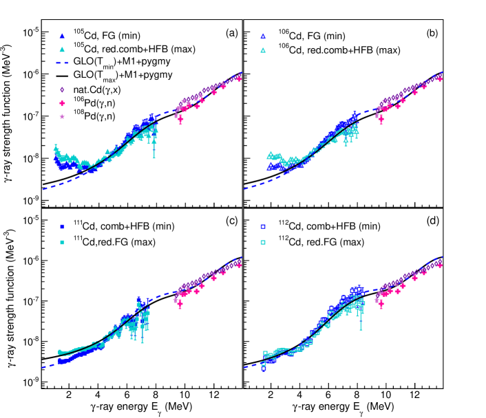
We observe that the models fit our data quite well, in particular for ^111,112Cd. The extra strength between $E_{\gamma}\approx 5-8$ MeV seems to be well described by a Gaussian function just as in the Sn case.

As of today, the origin of this strength is not well understood. It could be due to enhanced probability for $E1$ transitions due to the so-called neutron skin oscillation, see Refs. Sn_RSF ; Heidi_Sn2 and references therein. There is also a possibility that the $M1$ spin-flip resonance gives more strength than the parameterization we have adopted here. In a recent work on ⁹⁰Zr by Iwamoto et al. iwa90Zr , it is shown how both an $E1$ pygmy dipole resonance and an $M1$ resonance are present in the energy region $E_{\gamma}\approx 6-11$ MeV, with similar strengths. It could be that the same is the case also for the Cd isotopes. Unfortunately, with our experimental technique it is not possible to separate $E1$ and $M1$ transitions in the $\gamma$ strength. It would therefore be highly desirable to investigate this further with the experimental technique applied in Ref. iwa90Zr .

Assuming that all the pygmy strength is of $E1$ type, we have compared the energy-integrated strength of this structure with the classical energy-weighted Thomas-Reiche-Kuhn (TRK) sum rule (without exchange forces) given by TRK :

$$\sigma_{\mathrm{TRK}}\simeq 60\frac{NZ}{A}\>\left[{\mathrm{MeV\cdot mb}}\right].$$ (12)

The results are shown in Tab. 3.

Table 3: Maximum and minimum integrated strengths of the pygmy resonance.

Nucleus	$\sigma(T_{\mathrm{max}})$	$\sigma(T_{\mathrm{min}})$	TRK	% of TRK
	(MeV mb)	(MeV mb)	(MeV mb)
105Cd	11.3	21.8	1563.4	$0.7-1.4$
106Cd	11.3	24.4	1575.9	$0.7-1.5$
111Cd	17.4	28.7	1634.6	$1.1-1.8$
112Cd	24.4	37.4	1645.7	$1.5-2.3$

The uncertainty of the normalization gives a rather large uncertainty in the fraction of the sum rule, but the general trend is an increasing pygmy strength as the neutron number increases. This is in agreement with expectations based on the neutron-skin oscillation mode, see for example Ref. daoutidis .

We note that for ^105,106Cd, the models underestimate the strength for $E_{\gamma}<3$ MeV. Also, we find it not possible to compensate for this by just increasing $T_{f}$, because then the overall strength will be too large for the data at higher $\gamma$ energies. In an attempt to describe the extra strength at low $\gamma$ energies, we have tested a variable temperature of the final levels, $T_{f}\propto\sqrt{E_{f}}$, in the GLO model. This is shown as a solid, blue line in Fig. 10. It is seen that the variable-temperature model is rather successful in describing the low-energy data for the normalization giving the lowest low-energy strength.

It is however hard to explain why one should have a constant temperature for ^111,112Cd and a variable one for ^105,106Cd. By inspecting the level densities, they all have an approximately constant slope in log scale, compatible with a constant-temperature level density $\rho_{\mathrm{CT}}(E)\propto\exp(E/T)$. This has recently been supported by particle-evaporation experiments in lighter nuclei alex_rapid . In addition, the variable-temperature approach is not able to reproduce the data normalized to give maximum strength at low $\gamma$ energies (reduced spin range for the initial levels). We therefore conclude that it is more probable that some low-lying strength is present below $E_{\gamma}\approx 3.5$ MeV for ^105,106Cd, similar as for the Mo isotopes but not as strong. However, one must keep in mind that the uncertainty in the level-density normalization hampers any firm statements. Further studies of nuclei in this mass region are ongoing, and will hopefully shed more light on this issue.

V Summary and outlook

The level densities and $\gamma$-ray strength functions of ^{105,106,111,112}Cd have been deduced from particle-$\gamma$ coincidence data using the Oslo method. The level densities are in excellent agreement with known levels at low excitation energy. We note that the slope in level density decreases from the heavier ^111,112Cd to the lighter ^105,106Cd. This is probably due to the neutron number approaching the $N=50$ closed shell.

The $\gamma$-ray strength functions for all the Cd isotopes display an enhancement for $E_{\gamma}>4$ MeV, very similar to features observed in the previously studied Sn isotopes. The nature of this extra strength could not be determined in the present work, but could in principle be due to both $E1$ and $M1$ transitions. Future investigations are highly desirable to resolve these multi-polarities.

At $\gamma$-ray energies below 3 MeV, the $\gamma$-strength function of the lighter ^105,106Cd isotopes show an increase compared to ^111,112Cd. Although this might be due to the vicinity of the $N=50$ shell closure and the resulting reduced level density in the lighter isotopes, it is more likely that this work uncovered the mass region exhibiting the onset of the low-energy enhancement. Further measurements are in progress and the results will provide more details regarding this transitional region.