On the Convergence of Decentralized Gradient Descent

Abstract

Consider the consensus problem of minimizing $f(x)=\sum_{i=1}^{n}f_{i}(x)$, where $x\in\mathbb{R}^{p}$ and each $f_{i}$ is only known to the individual agent $i$ in a connected network of $n$ agents. To solve this problem and obtain the solution, all the agents collaborate with their neighbors through information exchange. This type of decentralized computation does not need a fusion center, offers better network load balance, and improves data privacy. This paper studies the decentralized gradient descent method [20], in which each agent $i$ updates its local variable $x_{(i)}\in\mathbb{R}^{n}$ by combining the average of its neighbors’ with a local negative-gradient step $-\alpha\nabla f_{i}(x_{(i)})$. The method is described by the iteration

$$x_{(i)}(k+1)\leftarrow\sum_{j=1}^{n}w_{ij}x_{(j)}(k)-\alpha\nabla f_{i}(x_{(i)}(k)),\quad\text{for each agent}~{}i,$$ (1)

where $w_{ij}$ is nonzero only if $i$ and $j$ are neighbors or $i=j$ and the matrix $W=[w_{ij}]\in\mathbb{R}^{n\times n}$ is symmetric and doubly stochastic.

This paper analyzes the convergence of this iteration and derives its rate of convergence under the assumption that each $f_{i}$ is proper closed convex and lower bounded, $\nabla f_{i}$ is Lipschitz continuous with constant $L_{f_{i}}>0$, and the stepsize $\alpha$ is fixed. Provided that $\alpha<O(1/L_{h})$, where $L_{h}=\max_{i}\{L_{f_{i}}\}$, the objective errors of all the local solutions and the network-wide mean solution reduce at rates of $O(1/k)$ until they reach a level of $O(\alpha)$. If $f_{i}$ are (restricted) strongly convex, then all the local solutions and the mean solution converge to the global minimizer $x^{*}$ at a linear rate until reaching an $O(\alpha)$-neighborhood of $x^{*}$. We also develop an iteration for decentralized basis pursuit and establish its linear convergence to an $O(\alpha)$-neighborhood of the true sparse signal. This analysis reveals how the convergence of (1) depends on the stepsize, function convexity, and network spectrum.

1 Introduction

Consider that $n$ agents form a connected network and collaboratively solve a consensus optimization problem

$$\operatorname*{minimize}\limits_{x\in\mathbb{R}^{p}}\quad f(x)=\sum_{i=1}^{n}f_{i}(x),$$ (2)

where each $f_{i}$ is only available to agent $i$. A pair of agents can exchange data if and only if they are connected by a direct communication link; we say that such two agents are neighbors of each other. Let ${\mathcal{X}}^{*}$ denote the set of solutions to (2), which is assumed to be non-empty, and let $f^{*}$ denote the optimal objective value.

The traditional (centralized) gradient descent iteration is

$$x(k+1)=x(k)-\alpha\nabla f(x(k)),$$ (3)

where $\alpha$ is the stepsize, either fixed or varying with $k$. To apply iteration (3) to problem (2) under the decentralized situation, one has two choices of implementation:

• let a fusion center (which can be a designated agent) carry out iteration (3);

• let all the agents carry out the same iteration (3) in parallel.

In either way, $f_{i}$ (and thus $\nabla f_{i}$) is only known to agent $i$. Therefore, in order to obtain $\nabla f(x(k))=\sum_{i=1}^{n}\nabla f_{i}(x(k))$, every agent $i$ must have $x(k)$, compute $\nabla f_{i}(x(k))$, and then send out $\nabla f_{i}(x(k))$. This approach requires synchronizing $x(k)$ and scattering/collecting $\nabla f_{i}(x(k))$, $i=1,\ldots,n$, over the entire network, which incurs a significant amount of communication traffic, especially if the network is large and sparse. A decentralized approach will be more viable since its communication is restricted to between neighbors. Although there is no guarantee that decentralized algorithms use less communication (as they tend to take more iterations), they provide better network load balance and tolerance to the failure of individual agents. In addition, each agent can keep its $f_{i}$ and $\nabla f_{i}$ private to some extent.

Decentralized gradient descent [20] does not rely on a fusion center or network-wide communication. It carries out an approximate version of (3) in the following fashion:

• let each agent $i$ hold an approximate copy $x_{(i)}\in\mathbb{R}^{p}$ of $x\in\mathbb{R}^{p}$;

• let each agent $i$ update its $x_{(i)}$ to the weighted average of its neighborhood;

• let each agent $i$ apply $-\nabla f_{i}(x_{(i)})$ to decrease $f_{i}(x_{(i)})$.

At each iteration $k$, each agent $i$ performs the following steps:

1. computes $\nabla f_{i}(x_{(i)}(k))$;

2. computes the neighborhood weighted average $x_{(i)}(k+1/2)=\sum_{j}w_{ij}x_{(j)}(k)$, where $w_{ij}\not=0$ only if $j$ is a neighbor of $i$ or $j=i$;

3. applies $x_{(i)}(k+1)=x_{(i)}(k+1/2)-\alpha\nabla f_{i}(x_{(i)}(k))$.

Steps 1 and 2 can be carried out in parallel, and their results are used in Step 3. Putting the three steps together, we arrive at our main iteration

$$\boxed{x_{(i)}(k+1)=\sum_{j=1}^{n}w_{ij}x_{(j)}(k)-\alpha\nabla f_{i}(x_{(i)}(k)),\quad i=1,2,\ldots,n.}$$ (4)

When $f_{i}$ is not differentiable, by replacing ${\nabla}f_{i}$ with a member of $\partial f_{i}$ we obtain the decentralized subgradient method [20]. Other decentralization methods are reviewed Section 1.2 below.

We assume that the mixing matrix $W=[w_{ij}]$ is symmetric and doubly stochastic. The eigenvalues of $W$ are real and sorted in a nonincreasing order $1=\lambda_{1}(W)\geq\lambda_{2}(W)\geq\cdots\geq\lambda_{n}(W)\geq-1$. Let the second largest magnitude of the eigenvalues of $W$ be denoted as

$$\beta=\max\left\{|\lambda_{2}(W)|,|\lambda_{n}(W)|\right\}.$$ (5)

The optimization of matrix $W$ and, in particular, $\beta$, is not our focus; the reader is referred to [4].

Some basic questions regarding the decentralized gradient method include: (i) When does $x_{(i)}(k)$ converge? (ii) Does it converge to $x^{*}\in{\mathcal{X}}^{*}$? (iii) If $x^{*}$ is not the limit, does consensus (i.e., $x_{(i)}(k)=x_{(j)}(k)$, $\forall i,j$) hold asymptotically? (iv) How do the properties of $f_{i}$ and the network affect convergence?

1.1 Background

The study on decentralized optimization can be traced back to the seminal work in the 1980s [30, 31]. Compared to optimization with a fusion center that collects data and performs computation, decentralized optimization enjoys the advantages of scalability to network sizes, robustness to dynamic topologies, and privacy preservation in data-sensitive applications [7, 17, 22, 32]. These properties are important for applications where data are collected by distributed agents, communication to a fusion center is expensive or impossible, and/or agents tend to keep their raw data private; such applications arise in wireless sensor networks [16, 24, 27, 38], multivehicle and multirobot networks [5, 26, 39], smart grids [10, 13], cognitive radio networks [2, 3], etc. The recent research interest in big data processing also motivates the work of decentralized optimization in machine learning [8, 28]. Furthermore, the decentralized optimization problem (2) can be extended to the online or dynamic settings where the objective function becomes an online regret [29, 32] or a dynamic cost [6, 12, 15].

To demonstrate how decentralized optimization works, we take spectrum sensing in a cognitive radio network as an example. Spectrum sensing aims at detecting unused spectrum bands, and thus enables the cognitive radios to opportunistically use them for data communication. Let $x$ be a vector whose elements are the signal strengths of spectrum channels. Each cognitive radio $i$ takes time-domain measurement $b_{i}=F^{-1}G_{i}x+e_{i}$, where $G_{i}$ is the channel fading matrix, $F^{-1}$ is the inverse Fourier transform matrix, and $e_{i}$ is the measurement noise. To each cognitive radio $i$, assign a local objective function $f_{i}(x)=(1/2)\|b_{i}-F^{-1}G_{i}x\|^{2}$ or the regularized function $f_{i}(x)=(1/2)\|b_{i}-F^{-1}G_{i}x\|^{2}+\phi(x)$, where $\phi(x)$ promotes a certain structure of $x$. To estimate $x$, a set of geologically nearby cognitive radios collaboratively solve the consensus optimization problem (2). Decentralized optimization is suitable for this application since communication between nearby cognitive radios are fast and energy-efficient and, if a cognitive radio joins and leaves the network, no reconfiguration is needed.

1.2 Related methods

The decentralized stochastic subgradient projection algorithm [25] handles constrained optimization; the fast decentralized gradient methods [11] adopts Nesterov’s acceleration; the distributed online gradient descent algorithm [29] has nested iterations, where the inner loop performs a fine search; the dual averaging subgradient method [8] carries out a projection operation after averaging and descending. Unsurprisingly, decentralized computation tends to require more assumptions for convergence than similar centralized computation. All of the above algorithms are analyzed under the assumption of bounded (sub)gradients. Unbounded gradients can potentially cause algorithm divergence. When using a fixed stepsize, the above algorithms (and iteration (4) in particular) converge to a neighborhood of $x^{*}$ rather than $x^{*}$ itself. The size of the neighborhood goes monotonic in the stepsize. Convergence to $x^{*}$ can be achieved by using diminishing stepsizes in [8, 11, 29] at the price of slower rates of convergence. With diminishing stepsizes, [11] shows an outer loop complexity of $O(1/k^{2})$ under Nesterov’s acceleration when the inner loop performs a substantial search job, without which the rate reduces to $O(\log(k)/k)$.

1.3 Contribution and notation

This paper studies the convergence of iteration (4) under the following assumptions.

Assumption 1.

1. For $i=1,\ldots,n$, $f_{i}$ is proper closed convex, lower bounded, and Lipschitz differentiable with constant $L_{f_{i}}>0$.

2. The network has a synchronized clock in the sense that (4) is applied to all the agents at the same time intervals, the network is connected, and the mixing matrix $W$ is symmetric and doubly stochastic with $\beta<1$ (see (5) for the definition of $\beta$).

Unlike [8, 11, 20, 25, 29], which characterize the ergodic convergence of $f(\hat{x}_{(i)}(k))$ where $\hat{x}_{(i)}(k)=\frac{1}{k}\sum_{s=0}^{k-1}{x}_{(i)}(s)$, this paper establishes the non-ergodic convergence of all local solution sequences $\{x_{(i)}(k)\}_{k\geq 0}$. In addition, the analysis in this paper does not assume bounded ${\nabla}f_{i}$. Instead, the following stepsize condition will ensure bounded $\nabla f_{i}$:

$$\alpha<O(1/L_{h}),$$ (6)

where $L_{h}=\max\{L_{f_{1}},\ldots,L_{f_{n}}\}$. This result is obtained through interpreting the iteration (4) for all the agents as a gradient descent iteration applied to a certain Lyapunov function.

Under Assumption 1 and condition (6), the rate of $O(1/k)$ for “near” convergence is shown. Specifically, the objective errors evaluated at the mean solution, $f(\frac{1}{n}\sum_{i=1}^{n}x_{(i)}(k))-f^{*}$, and at any local solution, $f({x}_{(i)}(k))-f^{*}$, both reduce at $O(1/k)$ until reaching the level $O(\frac{\alpha}{1-\beta})$. The rate of the mean solution is obtained by analyzing an inexact gradient descent iteration, somewhat similar to [8, 11, 20, 25]. However, all of their rates are given for the ergodic solution $\hat{x}_{(i)}(k)=\frac{1}{k}\sum_{s=0}^{k-1}{x}_{(i)}(s)$. Our rates are non-ergodic.

In addition, a linear rate of “near” convergence is established if $f$ is also strongly convex with modulus $\mu_{f}>0$, namely,

$$\langle\nabla f(x_{a})-\nabla f(x_{b}),x_{a}-x_{b}\rangle\geq\mu_{f}\|x_{a}-x_{b}\|^{2},\quad\forall x_{a},x_{b}\in{\mathrm{dom}}f,$$

or $f$ is restricted strongly convex [14] with modulus $\nu_{f}>0$,

$$\langle\nabla f(x)-\nabla f(x^{*}),x-x^{*}\rangle\geq\nu_{f}\|x-x^{*}\|^{2},\quad\forall x\in{\mathrm{dom}}f,~{}x^{*}={\mathrm{Proj}}_{{\mathcal{X}}^{*}}(x),$$ (7)

where ${\mathrm{Proj}}_{{\mathcal{X}}^{*}}(x)$ is the projection of $x$ onto the solution set ${\mathcal{X}}^{*}$ and $\nabla f(x^{*})=0$. In both cases, we show that the mean solution error $\|\frac{1}{n}\sum_{i=1}^{n}x_{(i)}(k)-x^{*}\|$ and the local solution error $\|x_{(i)}(k)-x^{*}\|$ reduce geometrically until reaching the level $O(\frac{\alpha}{1-\beta})$. Restricted strongly convex functions are studied as they appear in the applications of sparse optimization and statistical regression; see [37] for some examples. The solution set ${\mathcal{X}}^{*}$ is a singleton if $f$ is strongly convex but not necessarily so if $f$ is restricted strongly convex.

Since our analysis uses a fixed stepsize, the local solutions will not be asymptotically consensual. To adapt our analysis to diminishing stepsizes, significant changes will be needed.

Based on iteration (4), a decentralized algorithm is derived for the basis pursuit problem with distributed data to recover a sparse signal in Section 3. The algorithm converges linearly until reaching an $O(\frac{\alpha}{1-\beta})$-neighborhood of the sparse signal.

Section 4 presents numerical results on the test problems of decentralized least squares and decentralized basis pursuit to verify our developed rates of convergence and the levels of the landing neighborhoods.

Throughout the rest of this paper, we employ the following notations of stacked vectors:

$$[x_{(i)}]:=\begin{bmatrix}x_{(1)}\\ x_{(2)}\\ \vdots\\ x_{(n)}\end{bmatrix}\in\mathbb{R}^{np}\quad\text{and}\quad h(k):=\begin{bmatrix}\nabla f_{1}(x_{(1)}(k))\\ \nabla f_{2}(x_{(2)}(k))\\ \vdots\\ \nabla f_{n}(x_{(n)}(k))\end{bmatrix}\in\mathbb{R}^{np}.$$

2 Convergence analysis

2.1 Bounded gradients

Previous methods and analysis [8, 11, 20, 25, 29] assume bound gradients or subgradients of $f_{i}$. The assumption indeed plays a key role in the convergence analysis. For decentralized gradient descent iteration (4), it gives bounded deviation from mean $\|x_{(i)}(k)-\frac{1}{n}\sum_{j=1}^{n}x_{(j)}(k)\|$. It is necessary in the convergence analysis of subgradient methods, whether they are centralized or decentralized. But as we show below, the boundedness of $\nabla f_{i}$ does not need to be guaranteed but is a consequence of bounded stepsize $\alpha$, with dependence on the spectral properties of $W$. We derive a tight bound on $\alpha$ for $\nabla f_{i}(x_{(i)}(k))$ to be bounded.

Example. Consider $x\in\mathbb{R}$ and a network formed by 3 connected agents (every pair of agents are directly linked). Consider the following consensus optimization problem

$$\operatorname*{minimize}_{x}\ \ f(x)=\sum_{i=1,2,3}f_{i}(x),\quad\text{where}~{}f_{i}(x)=\frac{L_{h}}{2}(x-1)^{2},$$

and $L_{h}>0$. This is a trivial average consensus problem with $\nabla f_{i}(x_{(i)})=L_{h}(x_{(i)}-1)$ and $x^{*}=1$. Take any $\tau\in(0,1/3)$ and let the mixing matrix be

$$W=\begin{bmatrix}1-2\tau&\tau&\tau\\ \tau&\tau&1-2\tau\\ \tau&1-2\tau&\tau\end{bmatrix},$$

which is symmetric doubly stochastic. We have $\lambda_{3}(W)=3\tau-1\in(-1,0)$. Start from $(x_{(1)},x_{(2)},x_{(3)})=(1,0,2)$. Simple calculations yield:

• if $\alpha<(1+\lambda_{3}(W))/L_{h}$, then $x_{(i)}(k)$ converges to $x^{*}$, $i=1,2,3$; (The consensus among $x_{(i)}(k)$ as $k\to\infty$ is due to design.)

• if $\alpha>(1+\lambda_{3}(W))/L_{h}$, then $x_{(i)}(k)$ diverges and is asymptotically unbounded where $i=1,2,3$;

• if $\alpha=(1+\lambda_{3}(W))/L_{h}$, then $(x_{(1)}(k),x_{(2)}(k),x_{(3)}(k))$ equals $(1,2,0)$ at odd $k$ and $(1,0,2)$ at even $k$.

Clearly, if $x_{(i)}$ converges, then $\nabla f_{i}(x_{(i)})$ converges and thus stays bounded. In the above example $\alpha=(1+\lambda_{3}(W))/L_{h}$ is the critical stepsize.

As each $\nabla f_{i}(x_{(i)})$ is Lipschitz continuous with constant $L_{f_{i}}$, $h(k)$ is Lipschitz continuous with constant

$$L_{h}=\max_{i}\{L_{f_{i}}\}.$$

We formally show that $\alpha<(1+\lambda_{n}(W))/L_{h}$ ensures bounded $h(k)$. The analysis is based on the Lyapunov function

$$\xi_{\alpha}([x_{(i)}]):=-\frac{1}{2}\sum_{i,j=1}^{n}w_{ij}x_{(i)}^{T}x_{(j)}+\sum_{i=1}^{n}\left(\frac{1}{2}\|x_{(i)}\|^{2}+\alpha f_{i}(x_{(i)})\right),$$ (8)

which is convex since all $f_{i}$ are convex and the remaining terms $\frac{1}{2}\left(\sum_{i=1}^{n}\|x_{(i)}\|^{2}-\sum_{i,j=1}^{n}w_{ij}x_{(i)}^{T}x_{(j)}\right)$ is also convex (and uniformly nonnegative) due to $\lambda_{1}(W)=1$. In addition, $\nabla\xi_{\alpha}$ is Lipschitz continuous with constant $L_{\xi_{\alpha}}\leq(1-\lambda_{n}(W))+{\alpha}L_{h}$. Rewriting iteration (4) as

$$x_{(i)}(k+1)=\sum_{j=1}^{n}w_{ij}x_{(j)}(k)-\alpha\nabla f_{i}(x_{(i)}(k))=x_{(i)}(k)-\nabla_{i}\xi_{\alpha}([x_{(i)}(k)]),$$

we can observe that decentralized gradient descent reduces to unit-stepsize centralized gradient descent applied to minimize $\xi_{\alpha}([x_{(i)}])$.

Theorem 1.

Under Assumption 1, if the stepsize

$$\alpha\leq(1+\lambda_{n}(W))/L_{h},$$ (9)

then, starting from $x_{(i)}(0)=0$, ${i=1,2,\ldots,n}$, the sequence $x_{(i)}(k)$ generated by the iteration (4) converges. In addition we also have

$$\|h(k)\|\leq D:=\sqrt{2L_{h}\left(\sum_{i=1}^{n}f_{i}(0)-{f^{o}}\right)}$$ (10)

for all $k=1,2,\ldots$, where $f^{o}:=\sum_{i=1}^{n}f_{i}(x_{(i)}^{o})$ and $x_{(i)}^{o}=\arg\min_{x}f_{i}(x)$.

Proof.

Note that the iteration (4) is equivalent to the gradient descent iteration for the Lyapunov function (8). From the classic analysis of gradient descent iteration in [1] and [21], $[x_{(i)}(k)]$, and hence $x_{(i)}(k)$, will converge to a certain point when $\alpha\leq(1+\lambda_{n}(W))/L_{h}$.

Next we show (10). Since $\beta<1$, we have $\lambda_{n}(W)>-1$ and $(L_{\xi_{\alpha}}/2-1)\leq 0$. Hence,

$$\xi_{\alpha}([x_{(i)}(k+1)]) \leq\xi_{\alpha}([x_{(i)}(k)])+\nabla\xi_{\alpha}([x_{(i)}(k)])^{T}([x_{(i)}(k+1)-x_{(i)}(k)])+\frac{L_{\xi_{\alpha}}}{2}\|[x_{(i)}(k+1)-x_{(i)}(k)]\|^{2}$$

$$=\xi_{\alpha}([x_{(i)}(k)])+(L_{\xi_{\alpha}}/2-1)\|\nabla\xi_{\alpha}([x_{(i)}(k)])\|^{2}$$

$$\leq\xi_{\alpha}([x_{(i)}(k)]).$$

Recall that $\frac{1}{2}\left(\sum_{i=1}^{n}\|x_{(i)}\|^{2}-\sum_{i,j=1}^{n}w_{ij}x_{(i)}^{T}x_{(j)}\right)$ is nonnegative. Therefore, we have

$$\sum_{i=1}^{n}f_{i}(x_{(i)}(k))\leq\alpha^{-1}\xi_{\alpha}([x_{(i)}(k)])\leq\cdots\leq\alpha^{-1}\xi_{\alpha}([x_{(i)}(0)])=\alpha^{-1}\xi_{\alpha}(0)=\sum_{i=1}^{n}f_{i}(0).$$ (11)

On the other hand, for any differentiable convex function $g$ with the minimizer $x^{*}$ and Lipschitz constant $L_{g}$, we have $g(x_{a})\geq g(x_{b})+\nabla g^{T}(x_{b})(x_{a}-x_{b})+\frac{1}{2L_{g}}\|\nabla g(x_{a})-\nabla g(x_{b})\|^{2}$ and $\nabla g(x^{*})=0$. Then, $\|\nabla g(x)\|^{2}\leq 2L_{g}(g(x)-g^{*})$ where $g^{*}:=g(x^{*})$. Applying this inequality and (11), we obtain

$$\|h(k)\|^{2}=\sum_{i=1}^{n}\|\nabla f_{i}(x_{(i)}(k))\|^{2}\leq{\sum_{i=1}^{n}2L_{f_{i}}\left(f_{i}(x_{(i)}(k))-f_{i}^{o}\right)\leq 2L_{h}\left(\sum_{i=1}^{n}f_{i}(0)-f^{o}\right),}$$ (12)

where $f_{i}^{o}=f_{i}(x_{(i)}^{o})$ and $x_{(i)}^{o}=\arg\min_{x}f_{i}(x)$. Note that $x_{(i)}^{o}$ exists because of Assumption 1. Besides, we denote $f^{o}=\sum_{i=1}^{n}f_{i}^{o}$. This completes the proof. ∎

In the above theorem, we choose $x_{(i)}(0)=0$ for convenience. For general $x_{(i)}(0)$, a different bound for $\|h(k)\|$ can still be obtained. Indeed, if $x_{(i)}(0)\neq 0$, then $\alpha^{-1}\xi_{\alpha}(0)=\sum_{i=1}^{n}f_{i}(0)+\frac{1}{2\alpha}\big{(}\sum_{i=1}^{n}\|x_{(i)}(0)\|^{2}-\sum_{i,j=1}^{n}w_{ij}x_{(i)}(0)^{T}x_{(j)}(0)\big{)}$ in (11). Hence we have $\|h(k)\|^{2}\leq 2L_{h}\big{(}\sum_{i=1}^{n}f_{i}(0)-f^{o}\big{)}+\frac{L_{h}}{\alpha}\big{(}\sum_{i=1}^{n}\|x_{(i)}(0)\|^{2}-\sum_{i,j=1}^{n}w_{ij}x_{(i)}(0)^{T}x_{(j)}(0)\big{)}$. The initial values of $x_{(i)}(0)$ do not influence the stepsize condition though they change the bound of gradient. For simplicity, we let $x_{(i)}(0)=0$ in the rest of the paper.

Dependence on stepsize. In (4), the negative gradient step $-\alpha\nabla f_{i}(x_{(i)})$ does not diminish at $x_{(i)}=x^{*}$. Even if we let $x_{(i)}=x^{*}$ for all $i$, $x_{(i)}$ will immediately change once $\eqref{dec_grad}$ is applied. Therefore, the term $-\alpha\nabla f_{i}(x_{(i)})$ prevents the consensus of $x_{(i)}$. Even worse, because both terms in the right-hand side of (4) change $x_{(i)}$, they can possibly add up to an uncontrollable amount and cause $x_{(i)}(k)$ to diverge. The local averaging term is stable itself, so the only choice we have is to limit the size of $-\alpha\nabla f_{i}(x_{(i)})$ by bounding $\alpha$.

Network spectrum. One can design $W$ so that $\lambda_{n}(W)>0$ and thus simply bound (9) to

$$\alpha\leq 1/L_{h},$$

which no longer requires any spectral information of the underlying network. Given any mixing matrix $\tilde{W}$ satisfying $1=\lambda_{1}(\tilde{W})>\lambda_{2}(\tilde{W})\geq\cdots\geq\lambda_{n}(\tilde{W})>-1$ (cf. [4]), one can design a new mixing matrix $W=(\tilde{W}+I)/2$ that satisfies $1=\lambda_{1}(W)>\lambda_{2}(W)\geq\cdots\geq\lambda_{n}(W)>0$. The same argument applies to the results throughout the paper.

2.2 Bounded deviation from mean

Let

$$\bar{x}(k):=\frac{1}{n}\sum_{i=1}^{n}x_{(i)}(k)$$

be the mean of $x_{(1)}(k),\ldots,x_{(n)}(k)$. We will later analyze the error in terms of $\bar{x}(k)$ and then each $x_{(i)}(k)$. To enable that analysis, we shall show that the deviation from mean $\|x_{(i)}(k)-\bar{x}(k)\|$ is bounded uniformly over $i$ and $k$. Then, any bound of $\|\bar{x}(k)-x^{*}\|$ will give a bound of $\|x_{(i)}(k)-x^{*}\|$. Intuitively, if the deviation from mean is unbounded, then there would be no approximate consensus among $x_{(1)}(k),\ldots,x_{(n)}(k)$. Without this approximate consensus, descending individual $f_{i}(x_{(i)}(k))$ will not contribute to the descent of $f(\bar{x}(k))$ and thus convergence is out of the question. Therefore, it is critical to bound the deviation $\|x_{(i)}(k)-\bar{x}(k)\|$.

Lemma 1.

If (10) holds and $\beta<1$, then the total deviation from mean is bounded, namely,

$${{\|x_{(i)}(k)-\bar{x}(k)\|\leq\frac{\alpha D}{1-\beta},\quad\forall k,\forall i.}}$$

Proof.

Recall the definition of $[x_{(i)}]$ and $h(k)$, from the equation (4) we have

$$[x_{(i)}(k+1)]=(W\otimes I)[x_{(i)}(k)]-\alpha h(k),$$

where $\otimes$ denotes the Kronecker product. From it, we obtain

$$[x_{(i)}(k)]=-\alpha\sum_{s=0}^{k-1}(W^{k-1-s}\otimes I)h(s).$$ (13)

Besides, letting $[\bar{\mathbf{x}}(k)]=[\bar{x}(k);\cdots;\bar{x}(k)]\in\mathbb{R}^{np}$, it follows that

$$[\bar{x}(k)]=\frac{1}{n}((1_{n}1_{n}^{T})\otimes I))[\bar{\mathbf{x}}(k)].$$

As a result,

$$\|x_{(i)}(k)-\bar{x}(k)\| \leq\|[x_{(i)}(k)]-[\bar{\mathbf{x}}(k)]\|$$

$$=\|[x_{(i)}(k)]-\frac{1}{n}((1_{n}1_{n}^{T})\otimes I))[x_{(i)}(k)]\|$$

$$=\|-\alpha\sum\limits_{s=0}^{k-1}(W^{k-1-s}\otimes I)h(s)+\alpha\sum\limits_{s=0}^{k-1}\frac{1}{n}((1_{n}1_{n}^{T}W^{k-1-s})\otimes I)h(s)\|$$

$$=\|-\alpha\sum\limits_{s=0}^{k-1}(W^{k-1-s}\otimes I)h(s)+\alpha\sum\limits_{s=0}^{k-1}\frac{1}{n}((1_{n}1_{n}^{T})\otimes I)h(s)\|$$ (14)

$$=\alpha\|\sum\limits_{s=0}^{k-1}((W^{k-1-s}-\frac{1}{n}1_{n}1_{n}^{T})\otimes I)h(s)\|$$

$$\leq\alpha\sum\limits_{s=0}^{k-1}\|W^{k-1-s}-\frac{1}{n}1_{n}1_{n}^{T}\|\|h(s)\|$$

$$=\alpha\sum\limits_{s=0}^{k-1}\beta^{k-1-s}\|h(s)\|,$$

where (14) holds since $W$ is doubly stochastic. From $\|h(k)\|\leq D$ and $\beta<1$, it follows that

$$\|x_{(i)}(k)-\bar{x}(k)\|\leq\alpha\sum\limits_{s=0}^{k-1}\beta^{k-1-s}\|h(s)\|\leq\alpha\sum\limits_{s=0}^{k-1}\beta^{k-1-s}D\leq\frac{\alpha D}{1-\beta},$$

which completes the proof. ∎

The proof of Lemma 1 utilizes the spectral property of the mixing matrix $W$. The constant in the upper bound is proportional to the stepsize $\alpha$ and monotonically increasing with respect to the second largest eigenvalue modulus $\beta$. The papers [8], [20], and [25] also analyze the deviation of local solutions from their mean, but their results are different. The upper bound in [8] is given at the termination time of the algorithm, which is not uniform in $k$. The two papers [20] and [25], instead of bounding $\|W-\frac{1}{n}\mathbf{11}^{T}\|$, decompose it as the sum of element-wise $|w_{ij}-\frac{1}{n}|$ and then bounds it with the minimum nonzero element in $W$.

As discussed after Theorem 1, $D$ is affected by the value of $x_{(i)}(0)$, if it is nonzero. In Lemma 1, if $x_{(i)}(0)\neq 0$, then $[x_{(i)}(k)]=(W^{k}\otimes I)[x_{(i)}(0)]-\alpha\sum_{s=0}^{k-1}(W^{k-1-s}\otimes I)h(s)$. Substituting it into the proof of Lemma 1 we obtain

$$\|x_{(i)}(k)-\bar{x}(k)\|\leq\beta^{k}\|[x_{(i)}(0)]\|+\frac{\alpha D}{1-\beta}.$$

When $k\rightarrow\infty$, $\beta^{k}\|[x_{(i)}(0)]\|\rightarrow 0$ and, therefore, the last term dominates.

A consequence of Lemma 1 is that the distance between the following two quantities is also bounded

$$g(k) :=\frac{1}{n}\sum_{i=1}^{n}\nabla f_{i}(x_{(i)}(k)),$$

$$\bar{g}(k) :=\frac{1}{n}\sum_{i=1}^{n}\nabla f_{i}(\bar{x}(k)).$$

Lemma 2.

Under Assumption 1, if (10) holds and $\beta<1$, then

$$\|\nabla f_{i}(x_{(i)}(k))-\nabla f_{i}(\bar{x}(k))\| \leq\frac{\alpha DL_{f_{i}}}{1-\beta},$$

$$\|g(k)-\bar{g}(k)\| \leq\frac{\alpha DL_{h}}{1-\beta}.$$

Proof.

Assumption 1 gives

$$\|\nabla f_{i}(x_{(i)}(k))-\nabla f_{i}(\bar{x}(k))\|\leq L_{f_{i}}\|x_{(i)}(k)-\bar{x}(k)\|\leq\frac{\alpha DL_{f_{i}}}{1-\beta},$$

where the last inequality follows from Lemma 1. On the other hand, we have

$$\|g(k)-\bar{g}(k)\|=\|\frac{1}{n}\sum_{i=1}^{n}\big{(}\nabla f_{i}(x_{(i)}(k))-\nabla f_{i}(\bar{x}(k))\big{)}\|\leq\frac{1}{n}\sum_{i=1}^{n}L_{f_{i}}\|x_{(i)}(k)-\bar{x}(k)\|\leq\frac{\alpha DL_{h}}{1-\beta},$$

which completes the proof. ∎

We are interested in $g(k)$ since $-\alpha g(k)$ updates the average of $x_{(i)}(k)$. To see this, by taking the average of (4) over $i$ and noticing $W=[w_{ij}]$ is doubly stochastic, we obtain

$$\bar{x}(k+1)=\frac{1}{n}\sum_{i=1}^{n}x_{(i)}(k+1)=\frac{1}{n}{\sum_{i,j=1}^{n}}w_{ij}x_{(j)}-\frac{\alpha}{n}\sum_{i=1}^{n}\nabla f_{i}(x_{(i)}(k))=\bar{x}(k)-\alpha g(k).$$ (15)

On the other hand, since the exact gradient of $\frac{1}{n}\sum_{i=1}^{n}f_{i}(\bar{x}(k))$ is $\bar{g}(k)$, iteration (15) can be viewed as an inexact gradient descent iteration (using $g(k)$ instead of $\bar{g}(k)$) for the problem

$$\operatorname*{minimize}_{x}~{}\bar{f}(x):=\frac{1}{n}\sum_{i=1}^{n}f_{i}(x).$$ (16)

It is easy to see that $\bar{f}$ is Lipschitz continuous with the constant

$$L_{\bar{f}}=\frac{1}{n}\sum_{i=1}^{n}L_{f_{i}}.$$

If any $f_{i}$ is strongly convex, then so is $\bar{f}$, with the modulus $\mu_{\bar{f}}=\frac{1}{n}\sum_{i=1}^{n}\mu_{f_{i}}$. Based on the above interpretation, next we bound $f(\bar{x}(k))-f^{*}$ and $\|\bar{x}(k)-x^{*}\|$.

2.3 Bounded distance to minimum

We consider the convex, restricted strongly convex, and strongly convex cases. In the former two cases, the solution $x^{*}$ may be non-unique, so we use the set of solutions ${\mathcal{X}}^{*}$. We need the followings for our analysis:

• objective error $\bar{r}(k):=\bar{f}(\bar{x}(k))-\bar{f}^{*}=\frac{1}{n}(f(\bar{x}(k))-f^{*})~{}\text{where}~{}\bar{f}^{*}:=\bar{f}(x^{*})$, $x^{*}\in{\mathcal{X}}^{*}$;

• solution error $\bar{e}(k):=\bar{x}(k)-x^{*}(k)~{}\text{where}~{}x^{*}(k)={\mathrm{Proj}}_{{\mathcal{X}}^{*}}(\bar{x}(k))\in{\mathcal{X}}^{*}.$

Theorem 2.

Under Assumption 1, if $\alpha\leq\min\{(1+\lambda_{n}(W))/L_{h},1/L_{\bar{f}}\}=O(1/L_{h})$, then while

$$\bar{r}(k)>C\sqrt{2}\cdot\frac{\alpha L_{h}D}{(1-\beta)}=O\left(\frac{\alpha}{1-\beta}\right)$$

(where constants $C$ and $D$ are defined in (17) and (10), respectively), the reduction of $\bar{r}(k)$ obeys

$$\bar{r}(k+1)\leq\bar{r}(k)-O(\alpha\bar{r}^{2}(k)),$$

and therefore,

$$\bar{r}(k)\leq O\left(\frac{1}{\alpha k}\right).$$

In other words, $\bar{r}(k)$ decreases at a minimal rate of $O(\frac{1}{\alpha k})=O(1/k)$ until reaching $O(\frac{\alpha}{1-\beta})$.

Proof.

First we show that $\|\bar{e}(k)\|\leq C$. To this end, recall the definition of $\xi_{\alpha}([x_{(i)}])$ in (8). Let $\tilde{{\mathcal{X}}}$ denote its set of minimizer(s), which is nonempty since each $f_{i}$ has a minimizer due to Assumption 1. Following the arguments in [21, pp. 69] and with the bound on $\alpha$, we have $d(k)\leq d(k-1)\leq\cdots\leq d(0)$, where $d(k):=\|[x_{(i)}(k)-{\tilde{x}_{(i)}}]\|$ and $[\tilde{x}_{(i)}]\in\tilde{{\mathcal{X}}}$. Using $\|a_{1}+\cdots+a_{n}\|\leq\sqrt{n}\|{[a_{1};\ldots;a_{n}]}\|$, we have

$$\|\bar{e}(k)\| =\|\bar{x}(k)-x^{*}(k)\|=\|\frac{1}{n}\sum_{i=1}^{n}(x_{(i)}(k)-x^{*})\|\leq\frac{1}{\sqrt{n}}\|[x_{(i)}(k)-{x}^{*}]\|$$

$$\leq\frac{1}{\sqrt{n}}(\|{[x_{(i)}(k)-\tilde{x}_{(i)}]}\|+\|{[\tilde{x}_{(i)}-x^{*}]}\|)$$

$$\leq\frac{1}{\sqrt{n}}(\|{[x_{(i)}(0)-\tilde{x}_{(i)}]}\|+\|{[\tilde{x}_{(i)}-x^{*}]}\|)=:C$$ (17)

Next we show the convergence of $\bar{r}(k)$. By the assumption, we have $1-\alpha L_{\bar{f}}\geq 0$, and thus

$$\bar{r}(k+1) \leq\bar{r}(k)+\langle\bar{g}(k),\bar{x}({k+1})-\bar{x}(k)\rangle+\frac{L_{\bar{f}}}{2}\|\bar{x}({k+1})-\bar{x}(k)\|^{2}$$

$$\stackrel{{\scriptstyle\eqref{dec_avg}}}{{=}}\bar{r}(k)-\alpha\langle\bar{g}(k),g(k)\rangle+\frac{\alpha^{2}L_{\bar{f}}}{2}\|g(k)\|^{2}$$

$$=\bar{r}(k)-\alpha\langle\bar{g}(k),\bar{g}(k)\rangle+\frac{\alpha^{2}L_{\bar{f}}}{2}\|\bar{g}(k)\|^{2}+2\alpha\frac{1-\alpha L_{\bar{f}}}{2}\langle\bar{g}(k),\bar{g}(k)-g(k)\rangle+\frac{\alpha^{2}L_{\bar{f}}}{2}\|\bar{g}(k)-g(k)\|^{2}$$

$$\leq\bar{r}(k)-\alpha(1-\frac{\alpha L_{\bar{f}}}{2}-\delta\frac{1-\alpha L_{\bar{f}}}{2})\|\bar{g}(k)\|^{2}+\alpha(\frac{\alpha L_{\bar{f}}}{2}+\delta^{-1}\frac{1-\alpha L_{\bar{f}}}{2})\|\bar{g}(k)-g(k)\|^{2},$$

where the last inequality follows from Young’s inequality $\pm 2a^{T}b\leq\delta^{-1}\|a\|^{2}+\delta\|b\|^{2}$ for any $\delta>0$. Although we can later optimize over $\delta>0$, we simply take $\delta=1$. Since $\alpha\leq(1+\lambda_{n}(W))/L_{h}$, we can apply Theorem 1 and then Lemma 2 to the last term above, and obtain

$$\bar{r}(k+1)\leq\bar{r}(k)-\frac{\alpha}{2}\|\bar{g}(k)\|^{2}+\frac{\alpha^{3}D^{2}L_{h}^{2}}{2(1-\beta)^{2}}.$$

Since $\|\bar{e}(k)\|\leq C$ as shown in (17), from $\bar{r}(k)=\bar{f}(\bar{x}(k))-\bar{f}^{*}\leq\langle\bar{g}(k),\bar{x}(k)-x^{*}(k)\rangle=\langle\bar{g}(k),\bar{e}(k)\rangle$, we obtain that

$$\|\bar{g}(k)\|\geq\|\bar{g}(k)\|\frac{\|\bar{e}(k)\|}{C}\geq\frac{|\langle\bar{g}(k),\bar{e}(k)\rangle|}{C}\geq\frac{\bar{r}(k)}{C},$$

which gives

$$\bar{r}(k+1)\leq\bar{r}(k)-\frac{\alpha}{2C^{2}}\bar{r}^{2}(k)+\frac{\alpha^{3}D^{2}L_{h}^{2}}{2(1-\beta)^{2}}.$$

Hence, while $\frac{\alpha}{2C^{2}}\bar{r}^{2}(k)>2\cdot\frac{\alpha^{3}D^{2}L_{h}^{2}}{2(1-\beta)^{2}}$ or equivalently $\bar{r}(k)>C\sqrt{2}\cdot\frac{\alpha L_{h}D}{(1-\beta)}$, we have $\bar{r}(k+1)\leq\bar{r}(k)-O(\alpha\bar{r}^{2}(k))$. Dividing both sides by $\bar{r}(k)\bar{r}(k+1)$ gives $\frac{1}{\bar{r}(k)}+O(\frac{\alpha\bar{r}(k)}{\bar{r}(k+1)})\leq\frac{1}{\bar{r}(k+1)}$. Hence, $\frac{1}{\bar{r}(k)}$ increase at $\Omega(\alpha k)$, or $\bar{r}(k)$ reduces at $O(1/(\alpha k))$, which completes the proof. ∎

Theorem 2 shows that until reaching $f^{*}+O(\frac{\alpha}{1-\beta})$, $f(\bar{x}(k))$ reduces at the rate of $O(1/(\alpha k))$. For fixed $\alpha$, there is a tradeoff between the convergence rate and optimality. Again, upon the stopping of iteration (4), $\bar{x}(k)$ is not available to any of the agents but obtainable by invoking an average consensus algorithm.

Remark 1.

Since $\bar{f}(x)$ is convex, we have for all $i=1,2,\ldots,n$:

$$\bar{f}(x_{(i)}(k))-\bar{f}^{*} \leq\bar{r}(k)+\langle\bar{g}(x_{(i)}(k)),x_{(i)}(k)-\bar{x}(k)\rangle$$

$$\leq\bar{r}(k)+\frac{1}{n}\sum_{j=1}^{n}\|\nabla f_{j}(x_{(i)}(k))\|\|x_{(i)}(k))-\bar{x}(k)\|$$

$$\leq\bar{r}(k)+\frac{\alpha D^{2}}{1-\beta}.$$

From Theorem 2 we conclude that $\bar{f}(x_{(i)}(k))-\bar{f}^{*}$, like $\bar{r}(k)$, converges at $O(1/k)$ until reaching $O(\frac{\alpha}{1-\beta})$.

This nearly sublinear convergence rate is stronger than those of the distributed subgradient method [20] and the dual averaging subgradient method [8]. Their rates are in terms of objective error $f(\hat{x}_{(i)}(k))-f^{*}$ evaluated at the ergodic solution $\hat{x}_{(i)}(k)=\frac{1}{k}\sum_{s=0}^{k-1}x_{(i)}(s)$.

Next, we bound $\|\bar{e}(k+1)\|$ under the assumption of restricted or standard strong convexities. To start, we present a lemma.

Lemma 3.

Suppose that $\nabla\bar{f}$ is Lipschitz continuous with constant $L_{\bar{f}}$. Then, we have

$$\langle x-x^{*},{\nabla}\bar{f}(x)-{\nabla}\bar{f}(x^{*})\rangle\geq c_{1}\|{\nabla}\bar{f}(x)-{\nabla}\bar{f}(x^{*})\|^{2}+c_{2}\|x-x^{*}\|^{2}$$

(where $x^{*}\in{\mathcal{X}}^{*}$ and $\nabla\bar{f}(x^{*})=0$) for the following cases:

1. ([21, Theorem 2.1.12]) if ${\bar{f}}$ is strongly convex with modulus $\mu_{\bar{f}}$, then $c_{1}=\frac{1}{\mu_{\bar{f}}+L_{\bar{f}}}$ and $c_{2}=\frac{\mu_{\bar{f}}L_{\bar{f}}}{\mu_{\bar{f}}+L_{\bar{f}}}$;

2. ([37, Lemma 2]) if ${\bar{f}}$ is restricted strongly convex with modulus $\nu_{\bar{f}}$, then $c_{1}=\frac{\theta}{L_{\bar{f}}}$ and $c_{2}=(1-\theta)\nu_{\bar{f}}$ for any $\theta\in[0,1]$.

Theorem 3.

Under Assumption 1, if $f$ is either strongly convex with modulus $\mu_{f}$ or restricted strongly convex with modulus $\nu_{f}$, and if $\alpha\leq\min\{(1+\lambda_{n}(W))/L_{h},c_{1}\}=O(1/L_{h})$ and $\beta<1$, then we have

$$\|\bar{e}(k+1)\|^{2}\leq c_{3}^{2}\|\bar{e}(k)\|^{2}+c_{4}^{2},$$

where

$$c_{3}^{2}=1-\alpha c_{2}+\alpha\delta-\alpha^{2}\delta c_{2},\quad c_{4}^{2}=\alpha^{3}(\alpha+\delta^{-1})\frac{L_{h}^{2}D^{2}}{(1-\beta)^{2}},\quad D=\sqrt{2L_{h}\sum_{i=1}^{n}\left(f_{i}(0)-f_{i}^{o}\right)},$$

constants $c_{1}$ and $c_{2}$ are given in Lemma 3, $\mu_{\bar{f}}=\mu_{f}/n$ and $\nu_{\bar{f}}=\nu_{f}/n$, and $\delta$ is any positive constant. In particular, if we set $\delta=\frac{c_{2}}{2(1-\alpha c_{2})}$ such that $c_{3}=\sqrt{1-\frac{\alpha c_{2}}{2}}\in(0,1)$, then we have

$$\|\bar{e}(k)\|\leq c_{3}^{k}\|\bar{e}(0)\|+O(\frac{\alpha}{1-\beta}).$$

Proof.

Recalling that $x^{*}(k+1)={\mathrm{Proj}}_{{\mathcal{X}}^{*}}(\bar{x}(k+1))$ and $\bar{e}(k+1)=\bar{x}(k+1)-x^{*}(k+1)$, we have

$$\|\bar{e}(k+1)\|^{2} \leq\|\bar{x}(k+1)-x^{*}(k)\|^{2}$$

$$=\|\bar{x}(k)-x^{*}(k)-\alpha g(k)\|^{2}$$

$$=\|\bar{e}(k)-\alpha\bar{g}(k)+\alpha(\bar{g}(k)-g(k))\|^{2}\quad$$

$$=\|\bar{e}(k)-\alpha\bar{g}(k)\|^{2}+\alpha^{2}\|\bar{g}(k)-g(k)\|^{2}+2\alpha(\bar{g}(k)-g(k))^{T}(\bar{e}(k)-\alpha\bar{g}(k))$$

$$\leq(1+\alpha\delta)\|\bar{e}(k)-\alpha\bar{g}(k)\|^{2}+\alpha(\alpha+\delta^{-1})\|\bar{g}(k)-g(k)\|^{2},$$

where the last inequality follows again from $\pm 2a^{T}b\leq\delta^{-1}\|a\|^{2}+\delta\|b\|^{2}$ for any $\delta>0$. The bound of $\|\bar{g}(k)-g(k)\|^{2}$ follows from Lemma 2 and Theorem 1, and we shall bound $\|\bar{e}(k)-\alpha\bar{g}(k)\|^{2}$, which is a standard exercise; we repeat below for completeness. Applying Lemma 3 and noticing $\bar{g}(x)=\nabla{\bar{f}}(x)$ by definition, we have

$$\|\bar{e}(k)-\alpha\bar{g}(k)\|^{2} =\|\bar{e}(k)\|^{2}+\alpha^{2}\|\bar{g}(k)\|^{2}-2\alpha\bar{e}(k)^{T}\bar{g}(k)$$

$$\leq\|\bar{e}(k)\|^{2}+\alpha^{2}\|\bar{g}(k)\|^{2}-\alpha c_{1}\|\bar{g}(k)\|^{2}-\alpha c_{2}\|\bar{e}(k)\|^{2}$$

$$=(1-\alpha c_{2})\|\bar{e}(k)\|^{2}+\alpha(\alpha-c_{1})\|\bar{g}(k)\|^{2}.$$

We shall pick $\alpha\leq c_{1}$ so that $\alpha(\alpha-c_{1})\|\bar{g}(k)\|^{2}\leq 0$. Then from the last two inequality arrays, we have

$$\|\bar{e}(k+1)\|^{2} \leq(1+\alpha\delta)(1-\alpha c_{2})\|\bar{e}(k)\|^{2}+\alpha(\alpha+\delta^{-1})\|\bar{g}(k)-g(k)\|^{2}$$

$$\leq(1-\alpha c_{2}+\alpha\delta-\alpha^{2}\delta c_{2})\|\bar{e}(k)\|^{2}+\alpha^{3}(\alpha+\delta^{-1})\frac{L_{h}^{2}D^{2}}{(1-\beta)^{2}}.$$

Note that if $f$ is strongly convex, then $c_{1}c_{2}=\frac{\mu_{\bar{f}}L_{\bar{f}}}{(\mu_{\bar{f}}+L_{\bar{f}})^{2}}<1$; if $f$ is restricted strongly convex, then $c_{1}c_{2}=\frac{\theta(1-\theta)\nu_{\bar{f}}}{L_{\bar{f}}}<1$ because $\theta\in[0,1]$ and $\nu_{\bar{f}}<L_{\bar{f}}$. Therefore we have $c_{1}<1/c_{2}$. When $\alpha<c_{1}$, $(1+\alpha\delta)(1-\alpha c_{2})>0$.

Next, since

$$\|\bar{e}(k)\|^{2}\leq c_{3}^{2k}\|\bar{e}(0)\|^{2}+\frac{1-c_{3}^{2k}}{1-c_{3}^{2}}c_{4}^{2}\leq c_{3}^{2k}\|\bar{e}(0)\|^{2}+\frac{c_{4}^{2}}{1-c_{3}^{2}},$$

we get

$$\|\bar{e}(k)\|\leq c_{3}^{k}\|\bar{e}(0)\|+\frac{c_{4}}{\sqrt{1-c_{3}^{2}}}.$$

If we set

$$\delta=\frac{c_{2}}{2(1-\alpha c_{2})},$$

then we obtain

$$c_{3}^{2}=1-\frac{\alpha c_{2}}{2}<1,$$

$$\frac{c_{4}}{\sqrt{1-c_{3}^{2}}}=\frac{\alpha L_{h}D}{1-\beta}\sqrt{\frac{\alpha(\alpha+\frac{2(1-\alpha c_{2})}{c_{2}})}{\frac{\alpha c_{2}}{2}}}=\frac{\alpha L_{h}D}{1-\beta}\sqrt{\frac{4}{c_{2}^{2}}-\frac{2}{c_{2}}\alpha}=O(\frac{\alpha}{1-\beta}),$$

which completes the proof. ∎

Remark 2.

As a result, if $f$ is strongly convex, then $\bar{x}(k)$ geometrically converges until reaching an $O(\frac{\alpha}{1-\beta})$-neighborhood of the unique solution $x^{*}$; on the other hand, if $f$ is restricted strongly convex, then $\bar{x}(k)$ geometrically converges until reaching an $O(\frac{\alpha}{1-\beta})$-neighborhood of the solution set $\mathcal{X}^{*}$.

2.4 Local agent convergence

Corollary 1.

Under Assumption 1, if $f$ is either strongly convex or restricted strongly convex, $\alpha<\min\{(1+\lambda_{n}(W))/L_{h},c_{1}\}$ and $\beta<1$, then we have

$$\|x_{(i)}(k)-{x}^{*}(k)\|\leq c_{3}^{k}\|{x}^{*}(0)\|+\frac{c_{4}}{\sqrt{1-c_{3}^{2}}}+\frac{\alpha D}{1-\beta},$$

where $x^{*}(0),{x}^{*}(k)\in{\mathcal{X}}^{*}$ are solutions defined at the beginning of subsection 2.3 and the constants $c_{3}$, $c_{4}$, $D$ are the same as given in Theorem 3.

Proof.

From Lemma 1 and Theorem 3 we have

$$\|x_{(i)}(k)-{x}^{*}(k)\|$$

$$\leq \|\bar{x}(k)-{x}^{*}(k)\|+\|x_{(i)}(k)-\bar{x}(k)\|$$

$$\leq c_{3}^{k}\|{x}^{*}(0)\|+\frac{c_{4}}{\sqrt{1-c_{3}^{2}}}+\frac{\alpha D}{1-\beta},$$

which completes the proof. ∎

Remark 3.

Similar to Theorem 3 and Remark 1, if we set $\delta=\frac{c_{2}}{2(1-\alpha c_{2})}$, and if $f$ is strongly convex, then $x_{(i)}(k)$ geometrically converges to an $O(\frac{\alpha}{1-\beta})$-neighborhood of the unique solution $x^{*}$; if $f$ is restricted strongly convex, then $x_{(i)}(k)$ geometrically converges to an $O(\frac{\alpha}{1-\beta})$-neighborhood of the solution set $\mathcal{X}^{*}$.

3 Decentralized basis pursuit

3.1 Problem statement

We derive an algorithm for solving a decentralized basis pursuit problem to illustrate the application of iteration (4).

Consider a multi-agent network of $n$ agents who collaboratively find a sparse representation $y$ of a given signal $b\in\mathbb{R}^{p}$ that is known to all the agents. Each agent $i$ holds a part $A_{i}\in\mathbb{R}^{p\times q_{i}}$ of the entire dictionary $A\in\mathbb{R}^{p\times q}$, where $q=\sum_{i=1}^{n}q_{i}$, and shall recover the corresponding $y_{i}\in\mathbb{R}^{q_{i}}$. Let

$$y:=\left[\begin{array}[]{c}y_{1}\\ \vdots\\ y_{n}\end{array}\right]\in\mathbb{R}^{q},\quad A:=\left[\begin{array}[]{ccc}|&&|\\ A_{1}&\ldots&A_{n}\\ |&&|\end{array}\right]\in\mathbb{R}^{p\times q}.$$

The problem is

$$\operatorname*{minimize}\limits_{y} \quad\|y\|_{1},$$ (18)

subject to $$\quad\sum_{i=1}^{n}A_{i}y_{i}=b,$$

where $\sum_{i=1}^{n}A_{i}y_{i}=Ay$. This formulation is a column-partitioned version of decentralized basis pursuit, as opposed to the row-partitioned version in [19] and [36]. Both versions find applications in, for example, collaborative spectrum sensing [2], sparse event detection [18], and seismic modeling [19].

Developing efficient decentralized algorithms to solve (18) is nontrivial since the objective function is neither differentiable nor strongly convex, and the constraint couples all the agents. In this paper, we turn to an equivalent and tractable reformulation by appending a strongly convex term and solving its Lagrange dual problem by decentralized gradient descent. Consider the augmented form of (18) motivated by [14]:

$$\operatorname*{minimize}\limits_{y} \quad\|y\|_{1}+\frac{1}{2\gamma}\|y\|^{2},$$ (19)

subject to $$\quad Ay=b,$$

where the regularization parameter $\gamma>0$ is chosen so that (19) returns a solution to (18). Indeed, provided that $Ay=b$ is consistent, there always exists $\gamma_{\min}>0$ such that the solution to (19) is also a solution to (18) for any $\gamma\geq\gamma_{\min}$ [9, 33]. Linearized Bregman iteration proposed in [35] is proven to converge to the unique solution of (19) efficiently. See [33] for its analysis and [23] for important improvements. Since the problem (19) is now solved over a network of agents, we need to devise a decentralized version of linearized Bregman iteration.

The Lagrange dual of (19), casted as a minimization (instead of maximization) problem, is

$$\operatorname*{minimize}\limits_{x}~{}f(x):=\frac{\gamma}{2}\|A^{T}x-\text{Proj}_{[-1,1]}(A^{T}x)\|^{2}-b^{T}x,$$ (20)

where $x\in\mathbb{R}^{p}$ is the dual variable and $\text{Proj}_{[-1,1]}$ denotes the element-wise projection onto $[-1,1]$.

We turn (20) into the form of (2):

$$\operatorname*{minimize}_{x}~{}f(x)=\sum_{i=1}^{n}f_{i}(x),~{}\text{where}~{}f_{i}(x):=\frac{\gamma}{2}\|A_{i}^{T}x-\text{Proj}_{[-1,1]}(A_{i}^{T}x)\|^{2}-\frac{1}{n}b^{T}x.$$ (21)

The function $f_{i}$ is defined with $A_{i}$ and $b$, where matrix $A_{i}$ is the private information of agent $i$. The local objective functions $f_{i}$ are differentiable with the gradients given as

$$\nabla f_{i}(x)=\gamma A_{i}\text{Shrink}(A_{i}^{T}x)-\frac{b}{n},$$ (22)

where $\text{Shrink}(z)$ is the shrinkage operator defined as $\max(|z|-1,0)\mathrm{sign}(z)$ component-wise.

Applying the iteration (4) to the problem (21) starting with $x_{(i)}(0)=0$, we obtain the iteration

$$\boxed{x_{(i)}(k+1)=\sum_{j=1}^{n}w_{ij}x_{(j)}(k)-\alpha\left(A_{i}y_{i}(k)-\frac{b}{n}\right),\quad\text{where}~{}y_{i}(k)=\gamma\text{Shrink}(A_{i}^{T}x_{(i)}(k)).}$$ (23)

Note that the primal solution $y_{i}(k)$ is iteratively updated, as a middle step for the update of $x_{(i)}(k+1)$.

It is easy to verify that the local objective functions $f_{i}$ are Lipschitz differentiable with the constants $L_{f_{i}}=\gamma\|A_{i}\|^{2}$. Besides, given that $Ay=b$ is consistent, [14] proves that $f(x)$ is restricted strongly convex with a computable constant $\nu_{f}>0$. Therefore, the objective function $f(x)$ in (20) has $L_{h}=\max\{\gamma\|A_{i}\|^{2}:i=1,2,\cdots,n\}$, $L_{\bar{f}}=\frac{\gamma}{n}\sum_{i=1}^{n}\|A_{i}\|^{2}$ and $\nu_{\bar{f}}=\nu_{f}/n$. By Theorem 3, any local dual solution $x_{(i)}(k)$ generated by iteration (23) linearly converges to a neighborhood of the solution set of (20), and the primal solution $y(k)=[y_{1}(k);\cdots;y_{n}(k)]$ linearly converges to a neighborhood of the unique solution of (19).

Theorem 4.

Consider $x_{(i)}(k)$ generated by iteration (23) and $\bar{x}(k):=\frac{1}{n}\sum_{i=1}^{n}x_{(i)}(k)$. The unique solution of (19) is $y^{*}$ and the projection of $\bar{x}(k)$ onto the optimal solution set of (20) is $\bar{x}^{*}(k)=\text{Proj}_{\mathcal{X}^{*}}(\bar{x}(k))$. If the stepsize $\alpha<\min\{{(1+\lambda_{n}(W))}/{L_{h}},c_{1}\}$, we have

$$\|x_{(i)}(k)-\bar{x}^{*}(k)\|\leq c_{3}^{k}\|\bar{x}^{*}(0)\|+\left(\frac{c_{4}}{\sqrt{1-c_{3}^{2}}}+\frac{\alpha D}{1-\beta}\right),$$ (24)

where the constants $c_{3}$ and $c_{4}$ are the same as given in Theorem 3. In particular, if we set $\delta=\frac{c_{2}}{2(1-\alpha c_{2})}$ such that $c_{3}=\sqrt{1-\frac{\alpha c_{2}}{2}}\in(0,1)$, then $\frac{c_{4}}{\sqrt{1-c_{3}^{2}}}+\frac{\alpha D}{1-\beta}=O(\frac{\alpha}{1-\beta})$. On the other hand, the primal solution satisfies

$$\|y(k)-y^{*}\|\leq n\gamma\max_{i}\left(\|A_{i}\|\|x_{(i)}(k)-\bar{x}^{*}(k)\|\right).$$ (25)

Proof.

The result (24) is a corollary of Corollary 1. We focus on showing (25).

Given any dual solution $\bar{x}(k)$, the primal solution of (19) is $y^{*}=\gamma\text{Shrink}(A^{T}\bar{x}^{*}(k))$. Recall that $y(k)=[y_{1}(k);\cdots;y_{n}(k)]$ and $y_{i}(k)=\gamma\text{Shrink}(A_{i}^{T}x_{(i)}(k))$. We have

$$\|y(k)-y^{*}\|= \|[\gamma\text{Shrink}(A_{1}^{T}x_{(1)}(k));\cdots;\gamma\text{Shrink}(A_{n}^{T}x_{(n)}(k))]-\gamma\text{Shrink}(A^{T}\bar{x}^{*}(k))\|$$ (26)

$$\leq \gamma\sum_{i=1}^{n}\|\text{Shrink}(A_{i}^{T}x_{(i)}(k))-\text{Shrink}(A_{i}^{T}\bar{x}^{*}(k))\|.$$

Due to the contraction of the shrinkage operator, we have the bound $\|\text{Shrink}(A_{i}^{T}x_{(i)}(k))-\text{Shrink}(A_{i}^{T}\bar{x}^{*}(k))\|\leq\|A_{i}\|\|x_{(i)}(k)-\bar{x}^{*}(k)\|\leq\max_{i}\left(\|A_{i}\|\|x_{(i)}(k)-\bar{x}^{*}(k)\|\right)$. Combining this inequality with (26), we get (25). ∎

4 Numerical experiments

In this section, we report our numerical results applying the iteration (4) to a decentralized least squares problem and the iteration (23) to a decentralized basis pursuit problem.

We generate a network consisting of $n$ agents with $\frac{n(n-1)}{2}\eta$ edges that are uniformly randomly chosen, where $n=100$ and $\eta=0.3$ are chosen for all the tests. We ensure a connected network.

4.1 Decentralized gradient descent for least squares

We apply the iteration (4) to the least squares problem

$$\operatorname*{minimize}\limits_{x\in\mathbb{R}^{3}}\quad\frac{1}{2}\|b-Ax\|^{2}=\sum\limits_{i=1}^{n}\frac{1}{2}\|b_{i}-A_{i}x\|^{2}.$$ (27)

The entries of the true signal $x^{*}\in\mathbb{R}^{3}$ are i.i.d samples from the Gaussian distribution $\mathcal{N}(0,1)$. $A_{i}\in\mathbb{R}^{3\times 3}$ is the linear sampling matrix of agent $i$ whose elements are i.i.d samples from $\mathcal{N}(0,1)$, and $b_{i}=A_{i}x^{*}\in\mathbb{R}^{3}$ is the measurement vector of agent $i$.

For the problem (27), let $f_{i}(x)=\frac{1}{2}\|b_{i}-A_{i}x\|^{2}$. For any $x_{a},\ x_{b}\in\mathbb{R}^{3}$, $\|\nabla f_{i}(x_{a})-\nabla f_{i}(x_{b})\|=\|A_{i}^{T}A_{i}(x_{a}-x_{b})\|\leq\|A_{i}^{T}A_{i}\|\|x_{a}-x_{b}\|$, so $\nabla f_{i}(x)$ is Lipschitz continuous. In addition, $\frac{1}{2}\|b-Ax\|_{2}^{2}$ is strongly convex since $A$ has full column rank, with probability 1.

Fig. 1 depicts the convergence of the error $\bar{e}(k)$ corresponding to five different stepsizes. It shows that $\bar{e}(k)$ reduces linearly until reaching an $O(\alpha)$-neighborhood, which agrees with Theorem 3. Not surprisingly, a smaller $\alpha$ causes the algorithm to converge more slowly.

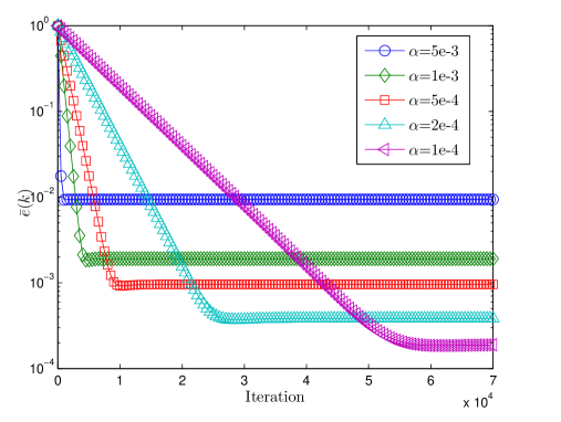
Figure 1: Comparison of different fixed stepsizes for the decentralized gradient descent algorithm.

Fig. 2 compares our theoretical stepsize bound in Theorem 1 to the empirical bound of $\alpha$. The theoretical bound for this experimental network is $\min\{\frac{1+\lambda_{n}(W)}{L_{h}},c_{1}\}=0.1038$. In Fig. 2, we choose $\alpha=0.1038$ and then the slightly larger $\alpha=0.12$. We observe convergence with $\alpha=0.1038$ but clear divergence with $\alpha=0.12$. This shows that our bound on $\alpha$ is quite close to the actual requirement.

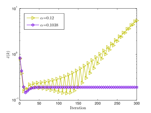
Figure 2: Comparison of the decentralized gradient descent algorithm with stepsizes $\alpha=0.1038$ and $\alpha=0.12$.

4.2 Decentralized gradient descent for basis pursuit

In this subsection we test the iteration (23) for the decentralized basis pursuit problem (18).

Let $y\in\mathbb{R}^{100}$ be the unknown signal whose entries are i.i.d. samples from $\mathcal{N}(0,1)$. The entries of the measurement matrix $A\in\mathbb{R}^{50\times 100}$ are also i.i.d. samples from $\mathcal{N}(0,1)$. Each agent $i$ holds the $i$th column of $A$. $b=Ay\in\mathbb{R}^{50}$ is the measurement vector. We use the same network as in the last test.

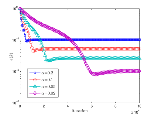
Figure 3: Convergence of the mean value of the dual variable $\bar{x}(k)$.

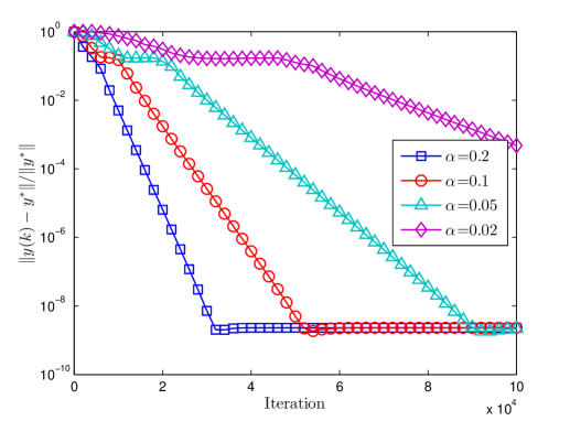
Figure 4: Convergence of the primal variable $y(k)$. $y^{*}$ is the solution of the problem (19).

Fig. 3 depicts the convergence of $\bar{x}(k)$, the mean of the dual variables at iteration $k$. As stated in Theorem 4, $\bar{x}(k)$ converges linearly to an $O(\alpha)$-neighborhood of the solution set $\mathcal{X}^{*}$. The limiting errors $\bar{e}(k)$ corresponding to the four values of $\alpha$ are proportional to $\alpha$. As the stepsize becomes smaller, the algorithm converges more accurately to $\mathcal{X}^{*}$. Fig. 4 shows the linear convergence of the primal variable $y(k)$. It is interesting that the $y(k)$ corresponding to three different values of $\alpha$ appear to reach the same level of accuracy, which might be related to the error forgetting property of the first-order $\ell_{1}$ algorithm [34] and deserves further investigation.

5 Conclusion

Consensus optimization problems in multi-agent networks arise in applications such as mobile computing, self-driving cars’ coordination, cognitive radios, as well as collaborative data mining. Compared to the traditional centralized approach, a decentralized approach offers more balanced communication load and better privacy protection. In this paper, our effort is to provide a mathematical understanding to the decentralized gradient descent method with a fixed stepsize. We give a tight condition for guaranteed convergence, as well as an example to illustrate the fail of convergence when the condition is violated. We provide the analysis of convergence and the rates of convergence for problems with different properties and establish the relations between network topology, stepsize, and convergence speed, which shed some light on network design. The numerical observations reasonably matches the theoretical results.

References

- [1] H. H. Bauschke and P. L. Combettes, Convex Analysis and Monotone Operator Theory in Hilbert Spaces, Springer, 2011.
- [2] J. A. Bazerque and G. B. Giannakis, Distributed spectrum sensing for cognitive radio networks by exploiting sparsity, IEEE Transactions on Signal Processing, 58 (2010), pp. 1847–1862.
- [3] J. A. Bazerque, G. Mateos, and G. B. Giannakis, Group-lasso on splines for spectrum cartography, IEEE Transactions on Signal Processing, 59 (2011), pp. 4648–4663.
- [4] S. Boyd, P. Diaconis, and L. Xiao, Fastest mixing markov chain on a graph, SIAM review, 46 (2004), pp. 667–689.
- [5] Y. Cao, W. Yu, W. Ren, and G. Chen, An overview of recent progress in the study of distributed multi-agent coordination, IEEE Transactions on Industrial Informatics, 9 (2013), pp. 427–438.
- [6] R. L. Cavalcante and S. Stanczak, A distributed subgradient method for dynamic convex optimization problems under noisy information exchange, IEEE Jounal of Selected Topics in Signal Processing, 7 (2013), pp. 243–256.
- [7] J. Chen and A. H. Sayed, Diffusion adaptation strategies for distributed optimization and learning over networks, IEEE Transactions on Signal Processing, 60 (2012), pp. 4289–4305.
- [8] J. C. Duchi, A. Agarwal, and M. J. Wainwright, Dual averaging for distributed optimization: convergence analysis and network scaling, IEEE Transactions on Automatic Control, 57 (2012), pp. 592–606.
- [9] M. P. Friedlander and P. Tseng, Exact regularization of convex programs, SIAM Journal on Optimization, 18 (2007), pp. 1326–1350.
- [10] G. B. Giannakis, V. Kekatos, N. Gatsis, S.-J. Kim, H. Zhu, and B. Wollenberg, Monitoring and optimization for power grids: A signal processing perspective, IEEE Signal Processing Magazine, 30 (2013), pp. 107–128.
- [11] D. Jakovetic, J. Xavier, and J. M. Moura, Fast distributed gradient methods, IEEE Transactions on Automatic Control, 59 (2014), pp. 1131–1146.
- [12] F. Jakubiec and A. Ribeiro, D-map: Distributed maximum a posteriori probability estimation of dynamic systems, IEEE Transactions on Signal Processing, 61 (2013), pp. 450–466.
- [13] V. Kekatos and G. B. Giannakis, Distributed robust power system state estimation, IEEE Transactions on Power Systems, 28 (2013), pp. 1617–1626.
- [14] M. Lai and W. Yin, Augmented and nuclear-norm models with a globally linearly convergent algorithm, SIAM Journal on Imaging Sciences, 6 (2013), pp. 1059–1091.
- [15] Q. Ling and A. Ribeiro, Decentralized dynamic optimization through the alternating direction method of multipliers, IEEE Transactions on Signal Processing, 62 (2014), pp. 1185–1197.
- [16] Q. Ling and Z. Tian, Decentralized sparse signal recovery for compressive sleeping wireless sensor networks, IEEE Transactions on Signal Processing, 58 (2010), pp. 3816–3827.
- [17] Q. Ling, Z. Wen, and W. Yin, Decentralized jointly sparse optimization by reweighted minimization, IEEE Transactions on Signal Processing, 61 (2013), pp. 1165–1170.
- [18] J. Meng, H. Li, and Z. Han, Sparse event detection in wireless sensor networks using compressive sensing, in IEEE Conference on Information Sciences and Systems, 2009, pp. 181–185.
- [19] J. F. Mota, J. M. Xavier, P. M. Aguiar, and M. Puschel, Distributed basis pursuit, IEEE Transactions on Signal Processing, 60 (2012), pp. 1942–1956.
- [20] A. Nedic and A. Ozdaglar, Distributed subgradient methods for multi-agent optimization, IEEE Transactions on Automatic Control, 54 (2009), pp. 48–61.
- [21] Y. Nesterov, Gradient methods for minimizing composite objective function, CORE report, (2007).
- [22] R. Olfati-Saber, J. A. Fax, and R. M. Murray, Consensus and cooperation in networked multi-agent systems, Proceedings of the IEEE, 95 (2007), pp. 215–233.
- [23] S. Osher, Y. Mao, B. Dong, and W. Yin, Fast linearized bregman iteration for compressive sensing and sparse denoising, Communications in Mathematical Sciences, 8 (2011), pp. 93–111.
- [24] J. B. Predd, S. Kulkarni, and H. V. Poor, Distributed learning in wireless sensor networks, IEEE Signal Processing Magazine, 23 (2006), pp. 56–69.
- [25] S. S. Ram, A. Nedic, and V. V. Veeravalli, Distributed stochastic subgradient projection algorithms for convex optimization, Journal of optimization theory and applications, 147 (2010), pp. 516–545.
- [26] W. Ren, R. W. Beard, and E. M. Atkins, Information consensus in multivehicle cooperative control, IEEE Control Systems Magazine, 27 (2007), pp. 71–82.
- [27] I. D. Schizas, A. Ribeiro, and G. B. Giannakis, Consensus in ad hoc wsns with noisy links – part i: Distributed estimation of deterministic signals, IEEE Transactions on Signal Processing, 56 (2008), pp. 350–364.
- [28] K. I. Tsianos, S. Lawlor, and M. G. Rabbat, Consensus-based distributed optimization: Practical issues and applications in large-scale machine learning, in IEEE Allerton Conference on Communication, Control, and Computing, 2012, pp. 1543–1550.
- [29] K. I. Tsianos and M. G. Rabbat, Distributed strongly convex optimization, in IEEE Conference on Communication, Control, and Computing, 2012, pp. 593–600.
- [30] J. Tsitsiklis, D. Bertsekas, and M. Athans, Distributed asynchronous deterministic and stochastic gradient optimization algorithms, IEEE Transactions on Automatic Control, 31 (1986), pp. 803–812.
- [31] J. N. Tsitsiklis, Problems in decentralized decision making and computation, MIT PhD Thesis, (1984).
- [32] F. Yan, S. Sundaram, S. Vishwanathan, and Y. Qi, Distributed autonomous online learning: regrets and intrinsic privacy-preserving properties, IEEE Transactions on Knowledge and Data Engineering, 25 (2013), pp. 2483–2493.
- [33] W. Yin, Analysis and generalizations of the linearized bregman method, SIAM Journal on Imaging Sciences, 3 (2010), pp. 856–877.
- [34] W. Yin and S. Osher, Error forgetting of bregman iteration, Journal of Scientific Computing, 54 (2013), pp. 684–695.
- [35] W. Yin, S. Osher, D. Goldfarb, and J. Darbon, Bregman iterative algorithms for -minimization with applications to compressed sensing, SIAM Journal on Imaging Sciences, 1 (2008), pp. 143–168.
- [36] K. Yuan, Q. Ling, W. Yin, and A. Ribeiro, A linearized bregman algorithm for decentralized basis pursuit, in European Signal Processing Conference, 2013.
- [37] H. Zhang and W. Yin, Gradient methods for convex minimization: better rates under weaker conditions, UCLA CAM Report, (2013).
- [38] F. Zhao, J. Shin, and J. Reich, Information-driven dynamic sensor collaboration, IEEE Signal Processing Magazine, 19 (2002), pp. 61–72.
- [39] K. Zhou and S. I. Roumeliotis, Multirobot active target tracking with combinations of relative observations, IEEE Transactions on Robotics, 27 (2011), pp. 678–695.