Lack of BV Bounds for Approximate Solutions to the p-system with Large Data

Abstract

We consider front tracking approximate solutions to the p-system of isentropic gas dynamics. At interaction times, the outgoing wave fronts have the same strength as in the exact solution of the Riemann problem, but some error is allowed in their speed. For large BV initial data, we construct examples showing that the total variation of these approximate solutions can become arbitrarily large, or even blow up in finite time. This happens even if the density of the gas remains uniformly positive.

1 Introduction

For hyperbolic systems of conservation laws in one space dimension, a satisfactory existence-uniqueness theory is currently available for entropy weak solutions with small total variation [2, 5]. The well-posedness of the Cauchy problem holds also in the case of large data, as long as the total variation remains bounded [3, 14]. A major remaining open problem is whether, for large BV initial data, the total variation remains uniformly bounded or can blow up in finite time. Examples of finite time blow up have been constructed in [1, 13]. However, these systems do not come from physical models and do not admit a strictly convex entropy.

For initial data having small total variation, regardless of the order in which wave fronts cross each other, the Glimm interaction estimates [9] show that the total strength of waves remains small for all times. There are few examples of hyperbolic systems where uniform BV estimates hold also for solutions with large data [17, 20]. In the present paper we study BV bounds for the p-system of isentropic gas dynamics in Lagrangean variables:

$$\left\{\begin{array}[]{rl}v_{t}-u_{x}&=~{}0\,,\cr u_{t}+p(v)_{x}&=~{}0\,.\end{array}\right.$$ (1.1)

Here $u$ is the velocity, $\rho$ is the density, $v=\rho^{-1}$ is specific volume, while $p=p(v)$ is the pressure. Our main concern is whether, for front tracking approximate solutions to the p-system, uniform BV estimates can be established. More precisely, we study the following question:

• Consider a front tracking approximation for (1.1) with large BV initial data. Assume that, at each interaction time, the outgoing wave fronts have the same strength as in the exact solution of the Riemann problem but some error is allowed in their speed. Can the total variation of such approximate solution become arbitrarily large?

In this paper, some examples will be constructed, showing that the total strength of waves in a front tracking approximation can indeed approach infinity in finite time. This confirms the non-existence of a Lyapunov functional which decreases at every wave-front interaction, as proved in [8].

For interactions occurring near vacuum, it was already noticed in [16] that uniform Glimm-type estimates were no longer valid. It thus comes as no surprise that an approximate front tracking solution can be constructed, where the total strength of waves (measured by the change in Riemann invariants) blows up in finite time. Remarkably, our last two examples show that an arbitrarily large amplification of the total variation is still possible even if the gas density remains uniformly positive.

It should be clear that the present counterexamples do not prove that, for large BV solutions of the $p$-system, the total variation can blow up in finite time. Indeed, we still conjecture that global BV bounds do hold. Our analysis only shows that such BV bounds cannot be proved by wave interaction estimates alone, and additional properties of solutions must be taken into account. Apparently, the decay of rarefaction waves due to genuine nonlinearity [2, 4, 6, 10] should be used in a crucial way. In the last section we revisit two of the earlier examples and show that, if such decay is taken into account, these specific interaction patterns do not produce blow up.

2 Wave interactions for the p-system

We review here some standard properties of characteristic curves and of shock curves. For details we refer to [8, 19]. To simplify the computations, we assume that in (1.1) the pressure has the special form

$$p(v)~{}=~{}{1\over 3v^{3}}~{}=~{}{\rho^{3}\over 3}\,,\qquad\qquad p^{\prime}(v)~{}=~{}-{1\over v^{4}}\,.$$

Smooth solutions of (1.1) satisfy the quasilinear system

$$\left\{\begin{array}[]{rl}\rho_{t}+\rho^{2}u_{x}&=~{}0,\cr\cr u_{t}+\rho^{2}\rho_{x}&=~{}0,\end{array}\right.$$ (2.1)

with characteristic speeds

$$\lambda~{}=~{}\pm\rho^{2}\,,$$ (2.2)

The variables

$$w_{1}~{}=~{}\rho-u\,,\qquad\qquad w_{2}~{}=~{}\rho+u\,,$$ (2.3)

provide a coordinate system of Riemann invariants, in the $u$-$\rho$ plane.

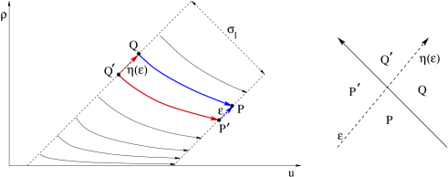
Figure 1: Interaction of a 1-shock and a 2-rarefaction

A shock with left state $(u_{-},\rho_{-})$ and right state $(u_{+},\rho_{+})$, traveling with speed $\lambda$, satisfies the Rankine-Hugoniot equations

$$\left\{\begin{array}[]{rl}\displaystyle\lambda\left({1\over\rho_{+}}-{1\over\rho_{-}}\right)&=~{}u_{-}-u_{+}\,,\cr&\cr\lambda(u_{+}-u_{-})&=~{}p(v_{+})-p(v_{-})~{}=\displaystyle~{}{\rho_{+}^{3}\over 3}-{\rho_{-}^{3}\over 3}\,.\end{array}\right.$$

Hence

$$u_{+}-u_{-}~{}=~{}-\sqrt{\left({1\over\rho_{+}}-{1\over\rho_{-}}\right)\left({\rho_{-}^{3}\over 3}-{\rho_{+}^{3}\over 3}\right)}\,,$$ (2.4)

$$\lambda~{}=~{}\pm{1\over\sqrt{3}}{\displaystyle\sqrt{\displaystyle{\rho^{3}_{-}}-{\rho^{3}_{+}}\over\displaystyle{1\over\rho_{+}}-{1\over\rho_{-}}}}\,.$$ (2.5)

Setting

$$s~{}=~{}u_{-}-u_{+}\,,\qquad\qquad\theta~{}=~{}{\rho_{+}\over\rho_{-}}\,,$$

from (2.4) it follows

$$s~{}=~{}\rho_{-}\,\sqrt{(1-\theta)(1-\theta^{3})\over 3\theta}\,.$$ (2.6)

For the p-system, the interaction of wave fronts has been thoroughly studied [19, 8]. For reader’s convenience, we derive here two elementary estimates which will be used in the sequel.

Consider a 1-shock with left and right states (see Fig. 1)

$$P~{}=~{}(u_{-},\rho_{-}),\qquad\qquad Q~{}=~{}(u_{+},\rho_{+})\,,$$

with strength

$$\sigma_{1}~{}=~{}|(\rho_{+}-u_{+})-(\rho_{-}-u_{-})|$$

measured by the change in the 1-Riemann invariant. Assume that this shock crosses a small 2-wave (compression or rarefaction) of strength $\sigma_{2}=\varepsilon$. We seek an estimate on the size of the outgoing waves, up to leading order. Let

$$P^{\prime}~{}=~{}(u_{-}-\varepsilon,\,\rho_{-}-\varepsilon),\qquad\qquad Q^{\prime}~{}=~{}\Big{(}u_{+}-\eta(\varepsilon),\,\rho_{+}-\eta(\varepsilon)\Big{)}$$

be the left and right states across the 1-shock after the interaction. Setting

$$s(\varepsilon)~{}=~{}s-\varepsilon+\eta(\varepsilon),\qquad\qquad\theta(\varepsilon)~{}=~{}{\theta\rho_{-}-\eta(\varepsilon)\over\rho_{-}-\varepsilon}\,,\qquad\qquad\psi(\theta)~{}=~{}{(1-\theta)(1-\theta^{3})\over 3\theta}$$ (2.7)

from (2.6) it follows

$$s(\varepsilon)~{}=~{}(\rho_{-}-\varepsilon)\,\sqrt{\psi(\theta(\varepsilon))}\,.$$ (2.8)

Differentiating w.r.t. $\varepsilon$, at $\varepsilon=0$ we obtain

$$\begin{array}[]{rl}\eta^{\prime}-1&\displaystyle=~{}-\sqrt{\psi(\theta)}+{\rho_{-}\over 2\sqrt{\psi(\theta)}}\cdot\psi^{\prime}(\theta)\theta^{\prime}\cr\cr&=\displaystyle-{s\over\rho_{-}}+{\rho_{-}^{2}\over 2s}\cdot{-1-2\theta^{3}+3\theta^{4}\over 3\theta^{2}}\cdot{\theta-\eta^{\prime}\over\rho_{-}}\,.\end{array}$$ (2.9)

Two cases are relevant to our analysis. CASE 1: The 1-shock has small amplitude. In this case, since shock and rarefaction curves coincide up to second order, for $s$ small we have the expansion

$$\theta~{}=~{}1+{s\over\rho_{-}}+{\cal O}(s^{3})\,.$$ (2.10)

Inserting (2.10) in (2.9) we obtain

$$\eta^{\prime}~{}=~{}1+\frac{1}{3}\left(\frac{s}{\rho_{-}}\right)^{3}+{\cal O}(s^{4})$$ (2.11)

CASE 2: The 1-shock has a fixed strength $\sigma_{1}$, while the density $\rho_{-}$ approaches zero. By definition, the strength is computed by

$$\sigma_{1}~{}=~{}(\theta-1)\rho_{-}+s~{}=~{}\left[(\theta-1)+\sqrt{\theta^{3}-\theta^{2}-1+\theta^{-1}\over 3}\right]\rho_{-}\,.$$ (2.12)

As $\rho_{-}\to 0$, from (2.12) it follows that $\theta\to\infty$. Indeed, dropping lower order terms we find

$${1\over\sqrt{3}}\theta^{3/2}\rho_{-}~{}\approx~{}\sigma_{1}\,,\qquad\qquad\theta~{}\approx~{}\left(\sqrt{3}\sigma_{1}\over\rho_{-}\right)^{2/3}\,.$$ (2.13)

Inserting (2.13) in (2.9) and retaining only leading order terms, we obtain

$$\eta^{\prime}-1~{}\approx~{}{-\sigma_{1}\over\rho_{-}}+{\rho_{-}\over 2\sigma_{1}}\cdot\theta^{2}\,(\theta-\eta^{\prime})\,,$$

$$\eta^{\prime}\approx~{}\frac{\displaystyle 1-\frac{\sigma_{1}}{\rho_{-}}+\frac{3}{2}\frac{\sigma_{1}}{\rho_{-}}}{\displaystyle 1+\frac{\rho_{-}}{2\sigma_{1}}\Big{(}\sqrt{3}\frac{\sigma_{1}}{\rho_{-}}\Big{)}^{4/3}}~{}\approx~{}\frac{1}{3^{2/3}}\Big{(}\frac{\sigma_{1}}{\rho_{-}}\Big{)}^{2/3},$$

$$\eta^{\prime}~{}\to~{}\infty\qquad\hbox{as}\quad\rho_{-}\to 0\,.$$ (2.14)

In other words, when an infinitesimal 2-wave crosses a 1-shock of fixed strength $\sigma_{1}$, its size is amplified by a factor $\eta^{\prime}\approx\kappa\,\rho_{-}^{-2/3}$ which becomes arbitrarily large as $\rho_{-}\to 0$, i.e. as the density approaches vacuum.

As a special case, if a 1-shock of strength $\sigma_{1}=1$ crosses a small 2-wave (either compression or rarefaction) of strength $\varepsilon\approx 0$, the strength of the shock remains constant, while the strength of the 2-wave is amplified by a factor

$${\eta(\varepsilon)\over\varepsilon}~{}>~{}{1\over\rho^{2/3}_{-}}\,.$$ (2.15)

The above estimate is valid as soon as the density $\rho_{-}$ of the left state (i.e., ahead of the 1-shock) is sufficiently small. One more case will be of relevance. Consider a small 1-shock with right state $(u_{+},\rho_{+})=(0,1)$. By (2.4) its left state $(u_{-},\rho_{-})$ satisfies

$$u_{-}~{}=~{}\sqrt{\left(1-{1\over\rho_{-}}\right){\rho_{-}^{3}-1\over 3}}\,.$$ (2.16)

Taking $\rho_{-}=1-s$, we obtain

$$u_{-}~{}=~{}\sqrt{\left(s^{2}-s^{3}+{s^{4}\over 3}\right)(1+s+s^{2}+\cdots)}~{}=~{}s\left(1+{s^{2}\over 6}+{s^{3}\over 6}+o(s^{3})\right)\,.$$ (2.17)

Next, consider a small 2-shock, again with right state $(\tilde{u}_{+},\tilde{\rho}_{+})=(0,1)$. Let $(\tilde{u}_{-},\tilde{\rho}_{-})$ be the left state. Taking $\tilde{\rho}_{-}=1+r$, by (2.16) we now have

$$\tilde{u}_{-}~{}=~{}\sqrt{\left(r^{2}+r^{3}+{r^{4}\over 3}\right)(1-r+r^{2}-\cdots)}~{}=~{}r\left(1+{r^{2}\over 6}-{r^{3}\over 6}+o(r^{3})\right)\,.$$ (2.18)

Imposing $u_{-}=\tilde{u}_{-}$ yields

$$r~{}=~{}s+{s^{4}\over 3}+o(s^{4}).$$

Referring to Fig. 5, consider the points

$$A_{1}=(0,1),\qquad C=(u_{-},\rho_{-}),\qquad D=(u_{-},\tilde{\rho}_{-}),$$

and let

$$B_{2}~{}=~{}\left(u_{-}+{\tilde{\rho}_{-}-\rho_{-}\over 2}\,,~{}{\tilde{\rho}_{-}+\rho_{-}\over 2}\right)~{}=~{}\left(2s+{s^{3}\over 6}+{s^{4}\over 3}+o(s^{4})\,,~{}1+{s^{4}\over 6}+o(s^{4})\right)$$

Then the slope of the segment $A_{1}B_{2}$ is

$${\displaystyle{s^{4}\over 6}+o(s^{4})\over\displaystyle 2s+{s^{3}\over 6}+{s^{4}\over 3}+o(s^{4})}~{}=~{}{s^{3}\over 12}+o(s^{3}).$$ (2.19)

3 Head-on interactions

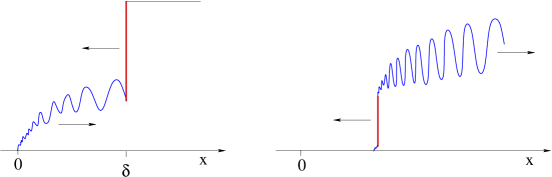
Figure 2: The head-on interaction of a 2-shock with a train of smooth 1-waves, in Example 1.

Example 1. Consider an initial data $(\bar{\rho},\bar{u})$ consisting of a 1-shock of strength $\sigma_{1}=1$, approaching a train of smooth 2-waves, near vacuum (Fig. 2).

In terms of Riemann invariants $(w_{1},w_{2})$, assume that the initial data is given by

$$\left\{\begin{array}[]{rl}w_{1}(0,x)&=~{}\bar{w}_{1}(x)~{}=~{}0\,,\cr w_{2}(0,x)&=~{}\bar{w}_{2}(x)~{}=~{}x^{\alpha}\cdot(2+\sin x^{-\beta})\end{array}\right.\qquad\hbox{for}~{}~{}x\in[0,\delta],$$ (3.1)

for suitable constants $\alpha,\beta>0$ and some $x_{0}>0$ suitably small. In addition, assume that this initial data has a 1-shock of size $\sigma_{1}=1$ at $x=1$, and is constant on the half lines where $x<0$ and $x>1$.

For this initial data we construct an approximate solution such that, at every interaction, the strength of outgoing waves is the same as in an exact solution. However, instead of (2.2) or (2.5), we let the waves travel with constant speeds, say, $-c$ for the 1-shock and $c$ for the 2-waves, for some constant $c>0$. Then, as $t\mapsto T=\delta/2c$, all the 2-waves cross the shock and the total variation of the solution approaches infinity. Indeed, by (2.15), choosing $\delta>0$ sufficiently small the following holds. At any time $0<t<T$ we have

$$\begin{array}[]{rl}|w_{2,x}(t,x+ct)|&\displaystyle\geq~{}{1\over\bar{\rho}(x)^{2/3}}\cdot|\bar{w}_{2,x}(x)|\cr\cr&\geq~{}\displaystyle{1\over\left(3x^{\alpha}/2\right)^{2/3}}\cdot\Big{|}\alpha x^{\alpha-1}(2+\sin x^{-\beta})-\beta x^{\alpha-\beta-1}\cos x^{-\beta}\Big{|},\end{array}$$ (3.2)

for all $x\in[0,x_{0}]$ such that $x+ct>1-ct$.

If we now choose $0<\alpha/3<\beta<\alpha<1$, then the initial data has bounded variation, because

$$\int_{0}^{1}|w_{2,x}(x)|\,dx~{}=~{}\int_{0}^{1}\Big{|}\alpha x^{\alpha-1}(2+\sin x^{-\beta})-\beta x^{\alpha-\beta-1}\cos x^{-\beta}\Big{|}\,dx~{}<~{}\infty.$$

On the other hand, as $t\to T-$ the total variation blows up, because

$$\begin{array}[]{l}\displaystyle\lim_{t\to 1/2c}\int_{1-2ct}^{x_{0}}|w_{2,x}(t,x+ct)|\,dx\cr\cr\qquad\displaystyle=~{}\left({2\over 3}\right)^{2\over 3}\int_{0}^{x_{0}}\Big{|}\alpha x^{(\alpha/3)-1}(2+\sin x^{-\beta})-\beta x^{(\alpha/3)-\beta-1}\cos x^{-\beta}\Big{|}\,dx~{}=~{}+\infty.\end{array}$$

In the previous example the initial data contains vacuum. Moreover, in the terminal profile the large variation is achieved at very low gas density. The next example shows that this arbitrarily large amplification of the total variation can be achieved also with an initial datum having uniformly positive density. As before, we require that at each interaction the strength of outgoing waves is the same as in an exact solution, but we allow a small error in the wave speed. Namely, in our approximate solution all 1-waves travel with speed $-c$ while 2-waves travel with speed $c$.

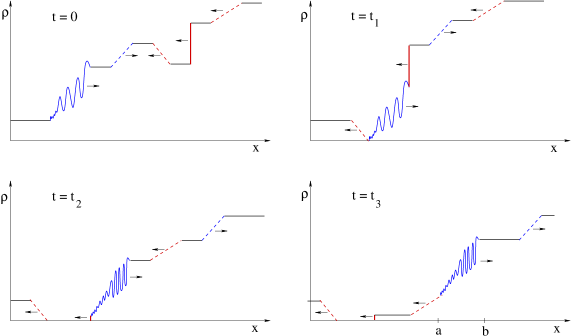
Figure 3: Evolution of the density profile in Example 2. Top left: at time $t=0$ the initial density is uniformly positive. Top right: after two rarefaction waves of the opposite families cross, in the middle section the same configuration in Example 1 is recreated. Bottom left: when the 1-shock crosses the train of 2-waves at low density, the total variation grows without bounds. Bottom right: after crossing a 1-compression, an arbitrarily large amount of total variation occurs within the interval $[a,b]$, at uniformly positive density.

Example 2. As shown in Fig. 3, consider an initial data similar to (3.1), but with the insertion of two additional rarefaction waves, and a compression. At time $t_{1}$, after crossing rarefaction waves of the opposite family, at time $t=t_{1}$ the train of 2-waves and the 1-shock recreate the initial data in Example 1. At time $t_{2}$, the total variation of the second Riemann invariant $w_{2}(t,\cdot)$ becomes infinite. At time $t_{3}$, after crossing a 1-compression, this infinite total variation occurs at uniformly positive density. In the $t$-$x$ plane, the solution is described in Fig. 4.

Remark 1. Example 2 shows that there exists an initial profile $(\bar{u},\bar{\rho})\in BV$ with $\bar{\rho}(x)\geq\rho_{0}>0$, and an approximate solution with fronts moving at constant speed $\pm c$ such that the following holds. If at each interaction the strength of outgoing waves is the same as in the exact solution of the Riemann problem, then the total variation blows up in finite time. More precisely, at some time $t_{3}$

$$\rho(t_{3},x)\geq 1\qquad\hbox{for}~{}~{}x\geq 0,\qquad\quad\hbox{Tot.Var.}\Big{\{}\rho(t_{3},\cdot)\,;~{}~{}[0,\infty[\,\Big{\}}~{}=~{}\infty.$$ (3.3)

In particular, is is not possible to put a continuous weight on wave strengths, possibly approaching infinity as $\rho\to 0$, in order to control the total variation. Indeed, for any choice of the weights, continuous on the region where $\rho>0$, the initial weighted total variation will be finite, while the final weighted total variation will be infinite.

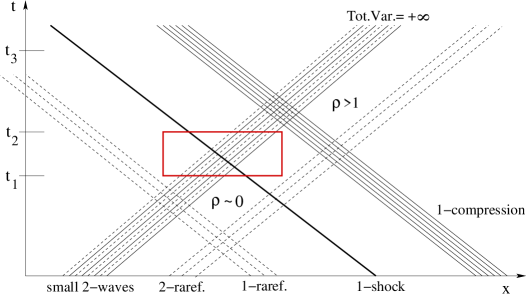
Figure 4: The wave pattern described in Example 2. The box shows the region where the interactions in Example 1 take place.

4 An example with uniformly positive density

In the previous examples, the blow up of the total variation was achieved because waves crossing a shock of unit strength were amplified by an arbitrarily large factor as the gas density approached vacuum. The following example shows that the total variation can become arbitrarily large even if the gas density remains uniformly bounded away from zero, at all times. Example 3. STEP 1. We begin by constructing a symmetric interaction pattern containing four wave fronts, as shown in Fig. 5. We choose the strengths of the two large shocks $S_{1},S_{2}$ and of the two intermediate waves in such a way that, after a whole round of interactions, these strengths are the same as at the initial time. Working in the $u$-$\rho$ plane, this is done as follows.

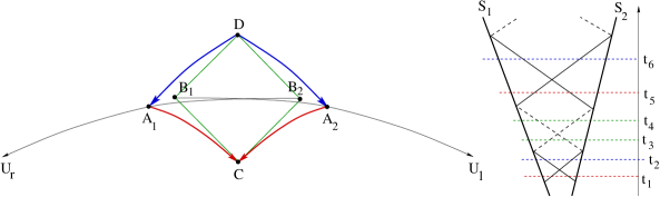
Figure 5: A periodic interaction pattern.

• Start by constructing two symmetric shocks: the 1-shock $A_{1}C$ and the 2-shock $A_{2}C$, approaching each other.

• Determine the two outgoing shocks $DA_{1}$ and $DA_{2}$, resulting from the crossing of the above two shocks.

• Construct a square having two opposite vertices at $C$ and $D$. Call $B_{1}$, $B_{2}$ the remaining two vertices.

• Choose $U_{l}$ so that the two points $B_{1}$ and $A_{2}$ are on the same 1-shock curve with left state $U_{l}$. Symmetrically, choose $U_{r}$ so that the two points $B_{2}$ and $A_{1}$ are on the same 2-shock curve with right state $U_{r}$.

The existence of states $U_{l}$, $U_{r}$ satisfying the conditions (iv) is now proved (see Fig. 6).

Lemma 1. In the $u$-$\rho$ plane, consider two points $B_{1}=(u_{1},\rho_{1})$ and $A_{2}=(u_{2},\rho_{2})$. Assume that

• $u_{1}<u_{2}$, and $\rho_{1}>\rho_{2}$.

• Calling $A=(u_{2},\rho_{2}^{*})$ the point on the 1-shock curve with right state $B_{1}$ with the same $u$-component as $A_{2}$, one has $\rho_{2}^{*}<\rho_{2}$.

Then there exists a unique $U_{l}=(u_{l},\rho_{l})$, with $0<\rho_{l}<\rho_{2}$, such that both $B_{1}$ and $A_{2}$ lie on the 1-shock curve with left state state $U_{l}$.

Proof. We shall use (2.4) with $(u_{-},\rho_{-})=(u_{l},\rho_{l})$ while $(u_{+},\rho_{+})=(u_{1},\rho_{1})$ or $(u_{+},\rho_{+})=(u_{2},\rho_{2})$. To prove the lemma we need to find $(u_{l},\rho_{l})$ such that

$$u_{l}-u_{1}~{}=~{}\sqrt{\left({1\over\rho_{1}}-{1\over\rho_{l}}\right)\left({\rho_{l}^{3}\over 3}-{\rho_{1}^{3}\over 3}\right)}\,,\qquad u_{l}-u_{2}~{}=~{}\sqrt{\left({1\over\rho_{2}}-{1\over\rho_{l}}\right)\left({\rho_{l}^{3}\over 3}-{\rho_{2}^{3}\over 3}\right)}\,.$$ (4.1)

Equivalently,

$$u_{2}-u_{1}~{}=~{}G(\rho_{l})~{}\doteq~{}\sqrt{\left({1\over\rho_{1}}-{1\over\rho_{l}}\right)\left({\rho_{l}^{3}\over 3}-{\rho_{1}^{3}\over 3}\right)}-\sqrt{\left({1\over\rho_{2}}-{1\over\rho_{l}}\right)\left({\rho_{l}^{3}\over 3}-{\rho_{2}^{3}\over 3}\right)}.$$ (4.2)

The assumption (ii) implies

$$G(\rho_{2})~{}=~{}\sqrt{\left({1\over\rho_{1}}-{1\over\rho_{l}}\right)\left({\rho_{l}^{3}\over 3}-{\rho_{1}^{3}\over 3}\right)}~{}<~{}u_{2}-u_{1}\,.$$

Moreover, a direct computation yields

$${\partial\over\partial\rho_{l}}G(\rho_{l})~{}<~{}0,\qquad\lim_{\rho_{l}\to 0}G(\rho_{l})~{}=~{}+\infty.$$

Therefore there exists a unique value of $\rho_{l}$ such that $G(\rho_{l})=u_{2}-u_{1}$. MM     

Figure 6: By moving the point $U$ along the 1-shock curve with right state $B_{1}$, we eventually reach a left state $U_{l}$ such that the 1-shock curve through $U_{l}$ contains $A_{2}$ as well.

Having constructed the above wave curves, consider the following interaction pattern, shown in Fig. 5, right:

• At time $t_{1}$ the initial datum consisting of four shocks, connecting the states $U_{l},A_{2},C,A_{1},U_{r}$.

• At time $t_{2}$ the profile still consists of four shocks (the two middle ones have crossed each other), connecting the states $U_{l},A_{2},D,A_{1},U_{r}$.

• At time $t_{3}$ the profile consists of two large shocks and two rarefactions (the two middle shocks have joined the big ones, generating two rarefactions), connecting the states $U_{l},B_{1},D,B_{2},U_{r}$.

• At time $t_{4}$ the profile still consists of two large shocks and two rarefactions (the two rarefactions have crossed each other), connecting the states $U_{l},B_{1},C,B_{2},U_{r}$.

• At time $t_{5}$ the initial datum consisting of four shocks (the two rarefactions have impinged on the big shocks, generating two intermediate shocks of the opposite families), connecting the states $U_{l},A_{2},C,A_{1},U_{r}$, exactly the same as at time $t_{1}$. The pattern thus repeats itself.

Remark 3. It is clear that for the above example it is essential to have large total variation. Indeed, if we choose the middle shock $A_{1}C$ small, then the line $A_{1}B_{2}$ will be almost horizontal and the point $U_{r}$ must be far away, with density close to zero.
On the other hand, in this solution obtained by front tracking the density trivially remains uniformly bounded away from zero. Since the interaction pattern is periodic, we conclude that Even under the assumption that the density remains uniformly positive, there is no way to construct a Lyapunov functional controlling the total variation, which is strictly decreasing at every interaction.

In the above approximate solution the wave strengths follow a periodic pattern. To achieve an arbitrarily large amplification of the total variation, a further construction is needed.

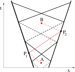
Figure 7: A periodic pattern that amplifies a small wave front.

STEP 2: As shown in Fig. 7, right, on top of the previous pattern we add a very small wave front. To fix the ideas, consider a 1-rarefaction of strength $\varepsilon>0$, located at $A$. Within a time period, this front will

• Cross the intermediate 2-shock.

• Interact with the large 1-shock at $P_{1}$ producing a 2-compression.

• Cross the intermediate 1-shock.

• Cross the intermediate 1-rarefaction.

• Interact with the large 2-shock at $P_{2}$ producing a 2-rarefaction.

• Cross the intermediate 2-rarefaction.

We analyze the case where the two middle shocks are small and the density of their left state is $\approx 1$. We claim that, when the additional front reaches $B$, its size will be increased by a factor $\kappa>1$.

Indeed, when a small wave of strength $\varepsilon^{-}$ crosses a shock of the opposite family of strength $s$ at density $\rho_{-}=1$, by (2.11) the strength of the outgoing front is

$$\varepsilon^{+}~{}=~{}\left(1+{s^{3}\over 3}+o(s^{3})\right)\varepsilon^{-}.$$ (4.3)

When the front crosses a rarefaction of the opposite family, its strength does not change.

Finally, when the small wave impinges on a large shock at $P_{1}$ or at $P_{2}$, we need to estimate the relative size of the reflected wave front. Toward this goal, let $\rho=\psi(u)$ be the equation of the shock curve with right state $U_{r}$, passing through both $A_{1}$ and $B_{2}$, as constructed in Lemma 1. Calling $\varepsilon^{-}$, $\varepsilon^{+}$ the strengths of the front before and after interaction, to leading order we have

$$\varepsilon^{+}~{}=~{}(1-2\psi^{\prime}(u))\varepsilon^{-}~{}=~{}\left(1-{s^{3}\over 6}+o(s^{3})\right)\varepsilon^{-}.$$ (4.4)

Indeed, by (2.19) we have $\psi^{\prime}(u)=s^{3}/12+o(s^{3})$. Calling $\varepsilon_{A}$ and $\varepsilon_{B}$ respectively the strengths of the small wave-front at $A$ and at $B$, we thus have

$$\varepsilon_{B}~{}=~{}\left(1+{s^{3}\over 3}+o(s^{3})\right)^{2}\left(1-{s^{3}\over 6}+o(s^{3})\right)^{2}\varepsilon_{A}~{}=~{}\left(1+{s^{3}\over 3}+o(s^{3})\right)\varepsilon_{A}\,.$$ (4.5)

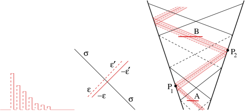
Figure 8: Right: a periodic pattern that amplifies infinitesimal waves. Center: if a front of strength $\sigma$ crosses a compression (not a shock!) of size $-\varepsilon$ and then a rarefaction of size $\varepsilon$, its final strength is not changed. The outgoing fronts have strengths $\varepsilon^{\prime},-\varepsilon^{\prime}$. Here $\varepsilon^{\prime}>\varepsilon$ if the front $\sigma$ is a shock, otherwise $\varepsilon^{\prime}=\varepsilon$. Left: to construct a interaction pattern that yields an arbitrarily large total variation, we replace the single infinitesimally small front in Fig. 7 by countably many pairs rarefaction + compression, of opposite size. The total strength of these waves is finite, each front having strength $\leq\varepsilon$.

STEP 3. Consider a periodic pattern that amplifies an infinitesimal wave, as in Step 2. By continuity, there exists $\lambda>1$ and $\varepsilon>0$ such that any wave-front (rarefaction or compression) of size $<\varepsilon$, traveling from $A$ to $B$ along the path in Fig. 7, is amplified by a factor $\geq\lambda$.

We now construct an initial set of wave fronts where the infinitesimal front is replaced by countably many pairs “rarefaction + compression”, whose sizes exactly cancel each other (Fig. 8, left). At time $t=0$, the total strength of all these small fronts can be taken to be $=1$. The key observation is that each of these pairs leaves no footprint on the underlying solution constructed in Step 1. Indeed, if a front of size $\sigma$ crosses a rarefaction and a compression of exactly opposite sizes, after the two crossings the size of the front is still $\sigma$ (Fig. 8, center). As a result, the pattern of four large fronts retains its periodicity.

By construction, after each period each pair of opposite small wavefronts is enlarged by a factor $\geq\lambda$. When a pair grows to size $>\varepsilon$, we can perform a partial cancellation so that its size remains $\in[\varepsilon/2,~{}\varepsilon]$.

Since the total number of small wave-fronts is infinite, after several periods a larger and larger number of pairs (compression + rarefaction) reaches size $>\varepsilon/2$. Hence, as $t\to\infty$, the total variation of this approximate solution grows without bounds.

5 Blow up in finite time

The previous construction shows that, if the total variation is initially sufficiently large, then there exists an interaction pattern that renders the total variation arbitrarily large as $t\to\infty$. This can be achieved even with a uniform lower bound on the density.

The next question is whether one can arrange the order of wave-front interactions so that the total variation blows up in finite time. Notice that this is not the case in the previous example. Indeed, if 1-fronts travel with speed $\dot{x}\in[-C,0[\,$ and 2-fronts travel with speed $\dot{x}_{2}\in\,]0,C]$, it takes a uniformly positive amount of time for each intermediate front to bounce back and forth between two large shocks. Hence the arbitrarily large amplification of the total variation is only achieved in the limit as $t\to+\infty$.

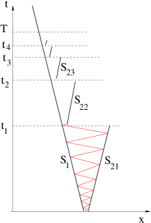
Figure 9: A pattern yielding finite time blow up of the total variation. At each step the total amount of small waves bouncing back and forth between the two large shocks keeps increasing.

In this section we briefly indicate how the previous construction can be modified, providing finite time blow up of the total variation. The main idea is illustrated in Fig. 9. We consider a sequence of times $0=t_{0}<t_{1}<t_{2}<\cdots<T$. During each time interval $J_{i}=[t_{i-1},t_{i}]$, a countable number of pairs of small waves (compression + rarefaction) is amplified by a very large factor. Before time $t_{i}$, the large 2-shock $S_{2i}$ is completely canceled by impinging 2-rarefactions, and a new 2-shock $S_{2(i+1)}$ of the same strength is recreated at a location closer to the large 1-shock $S_{1}$. Figures 10 and 11 show how this can be achieved, starting with very many pairs of small waves (compression + rarefaction). By letting each compression front collapse to a shock, and then canceling this shock with a rarefaction front of the same family, we obtain a train of pairs of small waves (compression + rarefaction) in the opposite family (Fig. 10, left). By varying the locations of these interactions, instead of many pairs of small waves we can achieve a large compression followed by a large rarefaction front (Fig. 10, right).

Figure 10: Starting with a large number of pairs of small waves, one can generate a large number of similar pairs in the other characteristic family (left), or one single large pair of fronts (right).

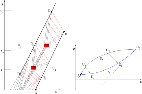
Figure 11: Left: between $A$ and $B$ the shock $S_{2}$ is completely canceled by impinging 2-rarefactions. Between $C$ and $D$, the new 2-shock $S_{2}^{\prime}$ is formed by impinging compression waves. Notice that the 1-compression fronts emerging from $S_{2}$ are used to completely cancel the 1-rarefactions that would otherwise be produced by the interactions of 2-compressions with $S_{2}^{\prime}$. Right: if the shock $S_{2}$ is very large, it cannot be canceled by one single large rarefaction front. Therefore, we need to produce several small rarefactions at subsequent times, so that the density $\rho$ remains uniformly positive.

The basic step is illustrated in Fig. 11. A large number of small compression+rarefaction pairs produces a large 2-rarefaction, which starts depleting the 2-shock along the line $AB$, and a large compression, which builds up a new 2-shock along the line $CD$. Since we cannot allow the density to become negative, it may not be possible to cancel the large shock $S_{2}$ with one single large 2-rarefaction. For this reason, this cancellation may be accomplished in several stages.

For example, the first set of 2-rarefactions reduce the size of the 2-shock $S_{2}$ from $(U_{\ell},U_{r})$ to $(U_{2},U_{r})$. At a time $\tau_{1}$, the profile $u(\tau_{1},\cdot)$ thus contains the 2-shock $(U_{\ell},U_{2})$, the 1-compression $(U_{2},U_{1})$, and the new 2-shock $(U_{1},U_{r})$.

At a later time $\tau_{2}$, the profile $u(\tau_{2},\cdot)$ contains the (shrinking) 2-shock $(U_{\ell},U_{4})$, the 1-compression $(U_{4},U_{3})$, and the (growing) 2-shock $(U_{3},U_{r})$.

At a later time $\tau_{3}$, the original 2-shock has been completely depleted by 2-rarefactions. A 2-shock connecting exactly the same two states $(U_{\ell},U_{r})$ is formed at a different location, as desired.

By canceling the large 2-shock and reconstructing it at a different location, shifted to the left, we can reproduce the pattern in Fig. 9. Since at each step the total strength of the small intermediate waves can be amplified by an arbitrarily large factor, as $t\to T$ the total variation of our approximate solution blows up to $+\infty$.

6 Concluding remarks

The examples presented in this paper show that, if the strength of wave-fronts is computed exactly but some error is allowed their speeds, then the total variation of approximate solutions can blow up. It is interesting to revisit some of the previous examples, taking into account the decay of rarefaction waves due to genuine nonlinearity. Looking at exact solutions, it becomes clear that these particular interaction patterns do not yield an arbitrarily large amplification of the total variation.

6.1 Head-on interactions, near vacuum.

Consider an exact solution of the system (1.1), with initial data as in Example 1. We show that there is no way to choose $\alpha,\beta$ in (3.1) so that the following requirements are simultaneously satisfied:

• The 1-shock crosses all 2-waves in finite time.

• The 2-waves do not break before crossing the shock.

• The sum of strengths of the 2-waves is initially finite, and becomes infinite as they all cross the 1-shock.

• The 2-waves do not break immediately after crossing the shock.

For a 1-shock of unit strength, assume that the left state (ahead of the shock) has density $\rho_{-}\approx 0$. Then by (2.4) the right state (behind the shock) has density $\rho_{+}$ satisfying

$${\rho_{+}^{3}\over 3}\cdot{1\over\rho_{-}}~{}\approx 1.$$

Hence the right state and the speed of the shock are given respectively by

$$\rho_{+}~{}\approx~{}(3\rho_{-})^{1/3}\,,\qquad\dot{x}~{}\approx~{}-{1\over\sqrt{3}}\sqrt{\rho_{+}^{3}\rho_{-}}~{}=~{}3^{-1/3}\,\rho_{-}^{2/3}.$$ (6.1)

If the initial profile is given by (3.1), so that

$$w_{1}(0,x)~{}=~{}0,\qquad w_{2}(0,x)~{}=~{}x^{\alpha}(2+\sin x^{-\beta})\qquad\qquad x\in[0,\delta],$$ (6.2)

then the requirement (i) will be satisfied provided that

$${2\over 3}\alpha~{}<~{}1\,.$$ (6.3)

Next, to make sure that the 2-waves do not break before crossing the 1-shock, we look at the evolution of $w_{2,x}$ along characteristics. From

$$w_{2,t}+\left({w_{2}\over 2}\right)^{2}w_{2,x}~{}=~{}0$$

it follows

$$w_{2,xt}+\left({w_{2}\over 2}\right)^{2}w_{2,xx}~{}=~{}-{w_{2}\over 4}\,w_{2,x}^{2}\,.$$

By a comparison argument, we conclude that the gradient $w_{2,x}$ will not blow up before time $T>0$ provided that the initial data satisfy

$$|w_{2,x}(0,x)|\cdot w_{2}(0,x)~{}<~{}T^{-1}.$$

Recalling (6.2), the condition (ii) is thus satisfied if

$$\alpha+(\alpha-\beta-1)~{}>~{}0\,.$$ (6.4)

As shown in the discussion of Example 1, condition (iii) is satisfied provided that

$$0~{}<~{}{\alpha\over 3}~{}<~{}\beta~{}<~{}\alpha~{}<~{}1.$$ (6.5)

To check whether (iv) can be satisfied, let $T$ be the time when the 1-shock reaches the origin, crossing all 2-waves. Denote by $t\mapsto x(t,y)$ the position of a 2-characteristic starting at $x(0,y)=y$, Calling $\tau(y)$ the time where this 2-characteristic crosses the 1-shock, we find

$$T-\tau(y)~{}\approx~{}y^{1-2\alpha/3}.$$

We consider the evolution of $w_{2,x}(t,x(t,y))$ along this 2-characteristic. For $t<\tau(y)$ we have

$$|w_{2,x}(t,x(t,y))|~{}\approx~{}y^{\alpha-\beta-1}.$$

When this characteristic crosses the 1-shock at time $\tau=\tau(y)$, by (2.15), this gradient is amplified by a factor

$${w_{2,x}(\tau+)\over w_{2,x}(\tau-)}~{}\approx~{}y^{-2\alpha/3}.$$

Moreover, $w_{2}(\tau+)\approx y^{\alpha/3}$. To make sure that this gradient remains bounded during the time interval $[\tau(y),T]$, we need

$$y^{-2\alpha/3}\cdot|w_{2,x}(\tau-)|\cdot w_{2}(\tau+)\,(T-t)~{}=~{}{\cal O}(1).$$

Therefore we should have

$$y^{-2\alpha/3}\cdot y^{\alpha-\beta-1}\cdot y^{\alpha/3}\cdot y^{1-2\alpha/3}~{}=~{}y^{-\beta}~{}=~{}{\cal O}(1).$$ (6.6)

This condition is incompatible with the requirement (6.5) that $\beta>0$.

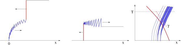
Figure 12: Left: Before crossing the large 1-shock, the small 2-waves do not break, because when the gas density $\rho>0$ is very small, the system is almost linearly degenerate. Center: after crossing the 1-shock, the 2-compression waves break and a large amount of cancellation between 2-rarefactions and 2-shocks occurs. At the terminal time $T$ the total strength of waves is still finite, due to these cancellations. Right: in the $t$-$x$ plane this pattern produces an infinite total variation only along the (dashed) time-like curve $\gamma$.

6.2 Waves bouncing back and forth between two large shocks

From our earlier analysis, this should be the pattern that achieves the greatest amplification of wave strengths (Fig. 13). If the size of the shocks $S_{1},S_{2}$ is sufficiently large, the strength of a reflected 2-front $\sigma^{\prime}$ is almost the same as the strength of the impinging 1-front $\sigma$. Afterwards, as this 2-front crosses other 1-shocks, its strength increases by a large factor. Repeating this pattern, it may appear that an arbitrarily large amplification of wave strengths can be achieved. The following analysis shows that this is not the case, if we take into account the decay of rarefaction waves due to genuine nonlinearity.

For some constant $c_{0}$, the two large shocks will have speeds

$$\dot{x}_{1}(t)~{}\leq~{}-c_{0}~{}<~{}0~{}<~{}c_{0}~{}\leq~{}\dot{x}_{2}(t)\,.$$ (6.7)

Consider a 1-rarefaction wave (Fig. 13) emerging from the large 2-shock at some time $\tau$ and impinging on the opposite 1-shock at time $\tau^{\prime}$. The upper and lower estimates on the velocity yield an estimate of the form

$$\tau^{\prime}~{}\geq~{}\kappa\tau\,.$$ (6.8)

By wave decay estimates, the density of such 1-rarefaction at time $\tau^{\prime}$ is

$$\leq~{}C\cdot{1\over\tau^{\prime}-\tau}~{}\leq~{}{C\kappa\over\kappa-1}\,{1\over\tau^{\prime}}\,.$$

Therefore, the total amount of 1-rarefactions that impinge on the large 1-shock within a time interval $[T_{0},T]$ is

$$\leq~{}\int_{T_{0}}^{T}{C\kappa\over\kappa-1}\,{1\over\tau^{\prime}}\,d\tau^{\prime}.$$

An entirely similar estimate holds for the 2-rarefactions impinging on the large 2-shock.

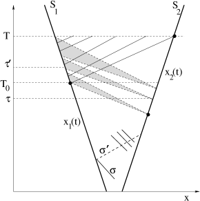
Figure 13: The total amount of compression waves (including shocks) at time $T$ is bounded in terms of the total amount of rarefaction waves that impinge on the large 1-shock during the interval $[T_{0},T]$.

Next, fix any large time $T$. As in Figure 13, consider the maximal backward 1-characteristic through the point $(T,x_{2}(T))$. This will cross the large 1-shock at an earlier time $T_{0}$. The total amount of 2-shocks (together with 2-compressions) at a given time $T$ can be estimated as:

$$\begin{array}[]{c}\hbox{Total amount of 2-shocks at time $T$ contained in the interval $[x_{1}(T),x_{2}(T)]$}\cr\cr=~{}{\cal O}(1)\cdot\hbox{amount of 1-rarefactions impinging on the 1-shock for $t\in[T_{0},\,T]$}\cr\cr\displaystyle=~{}{\cal O}(1)\cdot~{}\int_{T_{0}}^{T}{C\kappa\over\kappa-1}\,{1\over\tau^{\prime}}\,d\tau^{\prime}~{}=~{}{\cal O}(1)\cdot\ln{T\over T_{0}}~{}=~{}{\cal O}(1).\end{array}$$ (6.9)

Here ${\cal O}(1)$ denotes a quantity that remans uniformly bounded (provided that some upper and lower bounds on the density $\rho$ are given).

An entirely similar estimate of course holds for 1-shocks (together with 1-compressions). In addition, the rarefaction waves can be estimated as

$$\begin{array}[]{c}\hbox{total amount of 2-rarefactions at time $T$ contained in the interval $[x_{1}(T),x_{2}(T)]$}\cr\cr=~{}{\cal O}(1)\cdot\hbox{amount of 1-shocks impinging on the 1-shock for $t\in[T_{0},\,T]$}\cr\cr\leq~{}\hbox{total amount of 1-shocks at time $T_{0}$ contained in the interval $[x_{1}(T_{0}),x_{2}(T_{0})]$}~{}\leq~{}\hbox{const.}\cr\cr\end{array}$$ (6.10)

Here the last inequality follows from (6.9), with $T$ replaced by $T_{0}$. This yields a uniform a priori bound on the total strength of waves produced by this particular wave-interaction pattern.

References

- [1] P. Baiti and H. K. Jenssen, Blowup in for a class of genuinely nonlinear hyperbolic systems of conservation laws. Discrete Contin. Dynam. Systems 7 (2001), 837–853.
- [2] A. Bressan, Hyperbolic Systems of Conservation Laws. The One Dimensional Cauchy Problem. Oxford University Press, 2000.
- [3] A. Bressan and R. M. Colombo, Unique solutions of conservation laws with large data, Indiana Univ. Math. J. 44 (1995), 677–725.
- [4] A. Bressan and R. M. Colombo, Decay of positive waves in nonlinear systems of conservation laws, Ann. Scuola Normale Superiore Pisa IV - 26 (1998), 133–160.
- [5] A. Bressan, T. P. Liu and T. Yang, stability estimates for conservation laws, Arch. Rational Mech. Anal. 149 (1999), 1–22.
- [6] A. Bressan and T. Yang, A sharp decay estimate for positive nonlinear waves, SIAM Jour. Math. Anal. 36 (2004), 659-677.
- [7] T. Chang and L. Hsiao, The Riemann problem and interaction of waves in gas dynamics, Longman Scientific & Technical, Harlow, 1989.
- [8] G. Chen and H. K. Jenssen, No TVD fields for 1-d isentropic gas flow, Comm. Partial Differential Equations, 38 (2013), 629–657.
- [9] J. Glimm, Solutions in the large for nonlinear hyperbolic systems of equations, Comm. Pure Appl. Math. 18 (1965), 697–715.
- [10] J. Glimm and P. Lax, Decay of solutions of systems of nonlinear hyperbolic conservation laws, Amer. Math. Soc. Memoir 101 (1970).
- [11] D. Hoff, Invariant regions for systems of conservation laws. Trans. Amer. Math. Soc. 289 (1985), 591–610.
- [12] H. Holden and N. H. Risebro, Front Tracking for Hyperbolic Conservation Laws. Springer-Verlag, New York, 2002.
- [13] H. K. Jenssen, Blowup for systems of conservation laws, SIAM J. Math. Anal. 31 (2000), 894–908.
- [14] M. Lewicka, Well-posedness for hyperbolic systems of conservation laws with large BV data. Arch. Rational Mech. Anal. 173 (2004), 415–445.
- [15] L. W. Lin, On the vacuum state for the equations of isentropic gas dynamics. J. Math. Analysis Appl. 121 (1987), 406–425.
- [16] T. P. Liu and J. Smoller, On the vacuum state for the isentropic gas dynamics equations, Advances Pure Appl. Math. 1 (1980), 345–359.
- [17] T. Nishida, Global solution for an initial boundary value problem of a quasilinear hyperbolic system. Proc. Japan Acad. 44 (1968), 642–646.
- [18] O. Oleinik, Discontinuous solutions of nonlinear differential equations, Amer. Math. Soc. Transl. 26, 95–172.
- [19] J. Smoller, Shock waves and reaction-diffusion equations, Second edition. Springer-Verlag, New York, 1994.
- [20] B. Temple, Systems of conservation laws with invariant submanifolds, Trans. Amer. Math. Soc. 280 (1983), 781–795.