Optical/Near-IR Polarization Survey of Sh 2-29: Magnetic Fields,
Dense Cloud Fragmentations and Anomalous Dust Grain Sizes

Abstract

Sh 2-29 is a conspicuous star-forming region marked by the presence of massive embedded stars as well as several notable interstellar structures. In this research, our goals were to determine the role of magnetic fields and to study the size distribution of interstellar dust particles within this turbulent environment. We have used a set of optical and near-infrared polarimetric data obtained at OPD/LNA (Brazil) and CTIO (Chile), correlated with extinction maps, 2MASS data and images from DSS and Spitzer. The region’s most striking feature is a swept out interstellar cavity whose polarimetric maps indicate that magnetic field lines were dragged outwards, pilling up along its borders. This led to a higher magnetic strength value ($\approx 400\,\mu$G) and an abrupt increase in polarization degree, probably due to an enhancement in alignment efficiency. Furthermore, dense cloud fragmentations with peak $A_{V}$ between $20$ and $37$ mag were probably triggered by its expansion. The presence of $24\,\mu$m point-like sources indicates possible newborn stars inside this dense environment. A statistical analysis of the angular dispersion function revealed areas where field lines are aligned in a well-ordered pattern, seemingly due to compression effects from the Hii region expansion. Finally, Serkowski function fits were used to study the ratio of the total-to-selective extinction, reveling a dual population of anomalous grain particles sizes. This trend suggests that both effects of coagulation and fragmentation of interstellar grains are present in the region.

Accepted for The Astrophysical Journal

1. Introduction

It is well known that a large-scale magnetic field structure pervades the disk of the Milky Way Galaxy, including molecular clouds and star-forming regions (Mathewson & Ford, 1970; Novak et al., 1989, 1997; Heiles, 2000; Fosalba et al., 2002; Heiles & Crutcher, 2005; Santos et al., 2011). It is possible that the presence of these magnetic field lines play an important role on the initial stages of star-forming processes, providing support against the molecular cloud contraction. However, there is no general consent on whether these fields are important for the formation of sub-structures such as interstellar filaments, dense cores, and stars. On one hand, if magnetic fields are dynamically effective on this kind of environment, then star formation is probably regulated by the process known as ambipolar diffusion (Mestel & Spitzer, 1956; Nakano, 1979; Mouschovias & Paleologou, 1981; Shu et al., 1987; Lizano & Shu, 1989; Heitsch et al., 2004; Girart et al., 2009), or by the diffusion processes related to magnetic reconnection (Leão et al., 2012). On the other hand, if magnetic fields do not exert a very important role on these regions, then other effects, such as turbulence and stellar winds, must provide support against the collapse of molecular clouds (Padoan et al., 2004; Crutcher, 2005; McKee & Ostriker, 2007).

Furthermore, on later stages, there is clearly a very dynamical interaction between the newborn embedded stellar populations and their surrounding interstellar medium. This interaction significantly affects the morphology of gas and dust structures through radiation pressure and strong stellar winds, especially toward sites of massive star formation. Since the magnetic field is generally frozen within the interstellar gas, its lines are also critically affected in this process. The distortion of magnetic field lines due to such interaction, have been detected near some Galactic star-forming environments (e.g., Novak et al., 2000; Matthews et al., 2002; Kandori et al., 2007; Kusakabe et al., 2008; Tang et al., 2009; Santos et al., 2012). However, several open questions still remain, related to the importance of magnetic fields in determining the sizes of Hii regions, on the formation of radiation-driven filaments, and on the process of triggered star formation (Krumholz et al., 2007; Arthur et al., 2011).

The investigation of these questions is crucial to elucidate the underlying mechanisms controlling star formation. Unfortunately, when considering the widely different physical conditions of star-forming regions throughout the Galaxy, only few observations of magnetic fields are available. Therefore, in order to evaluate its general importance, it is pivotal to study this feature from stellar to Galactic scales. Such analyses should serve as essential tests to provide additional constraints to several star formation models.

The best tool to map the sky-projected lines of magnetic fields is obtained from interstellar polarization by aligned dust grains. Typically, due to the dissipation of internal energy from the interaction with the magnetic fields, the grains will be oriented with its major axis perpendicular to the field lines (Davis & Greenstein, 1951). Therefore, if stellar light goes through such dichroic interstellar environment, the beam will be linearly polarized following the magnetic field lines. This absorption effect is best observed using optical and near-infrared (near-IR) spectral bands.

Observations of several distinct spectral bands allow a particularly detailed analysis of magnetic fields, as well as the prevailing grain alignment mechanisms. Furthermore, by studying polarization as a function of wavelength it is possible to compute the distribution of grain sizes, which directly affects the interstellar extinction law (Gehrels & Silvester, 1965; Coyne, 1974; Serkowski et al., 1975; Codina-Landaberry & Magalhaes, 1976; Wilking et al., 1980; Messinger et al., 1997).

In this study we have focused on a rich star-forming region of the Galaxy, where the general aspects suggest a strong interaction between the stellar population and the magnetic field lines. In Section 2 we give a detailed description of this area, along with a listing of the majority of observations conducted toward its direction, available in the literature. Subsequently, Section 3 describes the observational methods and the polarimetric data. Sections 4 and 5 presents the results, analysis and discussion. Finally, the conclusions are shown in Section 6.

2. The Sh 2-29 star-forming region

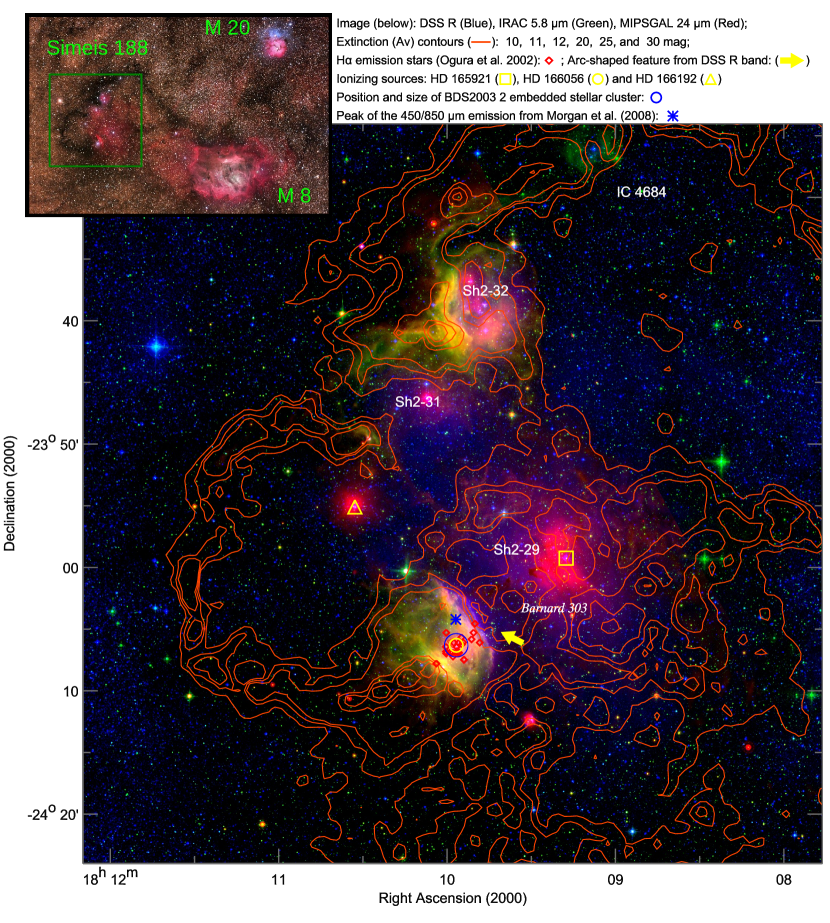
Figure 1.— Image of the Simeis 188 region (which includes Sh 2-29), represented by a combination of the following spectral bands: DSS R (blue), IRAC $5.8\,\mu$m (green), and MIPS $24\,\mu$m (red). The smaller image at the top shows a wider optical view of the region, also encompassing the M20 and M8 nebulae (source: http://www.nasaimages.org). Several stellar and interstellar features are marked, as specified by the indications at the top, and also detailed in Section 2. The extinction contours shown by the orange lines was obtained by using the 2MASS data, as described in Section 3.

The Sh 2-29 region was initially identified by Sharpless (1959), and classified as an irregular shape Hii region, displaying amorphous and filamentary structures (it is also known as NGC 6559 or IC 4685). This region is placed at the Simeis 188 Galactic complex, which is a rich star forming region at Sagittarius (near the direction of the Galactic center: $l\sim 7\arcdeg,b\sim-2\arcdeg$), including several bright nebulae, such as IC 1275 (Sh 2-31), IC 1274 (Sh 2-32) and IC 4684 (see Figure 1). According to Herbig (1957), Sh 2-29 is probably associated to the same complex of M8 (the Lagoon Nebula) and M20 (the Trifid Nebula).

Figure 1 is a combination of DSS R band (blue), Spitzer IRAC $5.8\,\mu$m (green), and Spitzer MIPS $24\,\mu$m (red) . Also overlaid on the image are the contours indicating the visual extinction $A_{V}$ (orange color, see Section 3). This area exhibits several interesting interstellar features, such as reflexion nebulae, dark clouds (e.g., the serpent-shaped structure Barnard 303), and H$\alpha$ emission from the ionized gas (which may be noticed, for example, as extended structures in blue – the R-band DSS image). The general interstellar morphology suggests a strong interaction between the embedded stellar population and the gas and dust structures.

Sharpless (1959) proposed that the Hii region’s main ionizing sources are the binary system HD165921 (spectral types O7v+O9v), HD166192 (B2ii), and HD166056 (B4i/ii), which are all relatively luminous stars in the visual band (V = 7.4, 8.5, and 9.7 mag, respectively). The $24\,\mu$m observations (red, Figure 1) show a strong extended emission mainly around HD165921 and HD166192, indicating a heating of the surrounding interstellar material (particularly near HD165921, an arc-shaped structure may be noticed).

Thermal emission from the radio continuum (2695 GHz), which is typically related to free-free emission, was detected toward Sh 2-29 by Altenhoff et al. (1970). Other radio observations were carried out aiming at obtaining radial velocities based on CO lines (Blitz et al., 1982). Assuming a Galaxy rotation model (Fich & Blitz, 1984), a distance of $d=1.3\pm 0.5$ kpc was computed. CO-line studies have also been carried out by Yamaguchi et al. (1999), who interpreted the entire Sh 2-29 interstellar complex as an expanding shell. By assuming an expansion velocity of 5 km s^-1 and a 5-10 pc radius, a dynamical age of 1-2 million years was estimated. Other studies of Sh 2-29 include far ultraviolet observations (Carruthers & Page, 1984), as well as analysis of H$\alpha$ spectra (Fich et al., 1990).

Although Sh 2-29 seems related to other nearby Hii regions, the presence of different CO velocities suggests different distances. In fact, for M8 and M20, recent distance estimates suggest respectively 1250 and 1670 pc (Arias et al., 2007; Rho et al., 2008), although variations in the extinction law toward the Trifid Nebula (M20) may indicate a somewhat higher distance of $2.7\pm 0.5$ kpc (Cambrésy et al., 2011). Toward Sh 2-32, which is positioned $\approx$25 arcmin North of Sh 2-29 (and is supposedly part of the same interstellar complex), Dahm et al. (2012) have determined a distance of $1.8\pm 0.3$ kpc for the associated bright stellar cluster, which is consistent with other photometric and kinematic distance indicators (Georgelin et al., 1973; Vogt & Moffat, 1975; Fich & Blitz, 1984; Oka et al., 1999).

By using data from the 2MASS near-IR survey Bica et al. (2003) found an embedded stellar cluster surrounding the ionizing source HD166056, denominated BDS2003 2 (with an angular dimension of $1.9^{\prime}$). The cluster is at the center of a prominent cavity only seen in the mid/far-IR images (green/yellow emission from Figure 1). Around this cavity, a large arc-shaped interstellar shell is visible in the DSS R-band image, and therefore is likely an expanding ionization front (assuming such feature is mainly due to the H$\alpha$ emission). Ogura et al. (2002) observed 23 H$\alpha$-emission sources toward this cluster, a feature which is typical of pre-main sequence objects (e.g., T Tauri or Herbig Ae/Be stars).

Morgan et al. (2008) conducted SCUBA sub-mm observations toward Sh 2-29 (450 and 850 $\,\mu$m), revealing an extended dust emission feature $\approx$2 arcmin North of the BDS2003 2 cluster’s center, coinciding with the position of the IRAS 18068-2405 source. Urquhart et al. (2009) carried out CO observations complemented with MSX and Spitzer data, concluding that no mid-IR point source may be detected toward this feature, and therefore the region is still in a very early evolutionary stage, with most of its luminosity still in the sub-mm range. Furthermore, it is suggested that star formation activity at this interstellar structure has possibly been externally triggered. Urquhart et al. (2009) concluded that its current evolutionary status corresponds to the phase immediately after the emergence and exposition to an external ionization front, and before the arising of the first proto-stellar objects with significant mid-IR emission.

The only known polarimetric study of a region close to Sh 2-29 was conducted by McCall et al. (1990) toward M8, which is located at approximately $1.6^{\circ}$ from it. They have found a significantly anomalous value of the total-to-selective extinction ratio of $R=4.6\pm 0.3$, which is probably due to effects of evaporation and coagulation of interstellar grain particles. Moreover, according to the interpretation of McCall et al. (1990), the overall cloud’s morphology suggests a previous gravitational collapse following the magnetic field lines.

3. Observational data

The linear polarization data used in this work are a combination of observations conducted at the Cerro Tololo Interamerican Observatory (CTIO, Chile), using the 0.9 m telescope, and also at the Observatório Pico dos Dias/Laboratório Nacional de Astrofísica (OPD/LNA, Brazil), using both the 0.6 m and the 1.6 m telescopes. The optical data (V, R, and I Johnson-Cousins bands) were obtained with the CTIO-0.9 m and OPD-0.6 m telescopes, while the near-IR data (H band) were collected with the OPD-1.6 m telescope.

A brief description of the instrument and the data reduction process is given here. For a complete and detailed discussion, see Santos et al. (2012). The polarimetric modules used in this work, from both OPD and CTIO, basically consist of a sequence of optical elements positioned in the stellar light path, before the beam reaches the detector. Assuming that the polarization orientation is defined by an angle $\theta$ relative to the North Celestial Pole, initially a half-wave plate causes a rotation of the polarization plane. The plate itself may be rotated in discrete steps of $22.5\arcdeg$, resulting in consecutive polarization plane rotations of $45\arcdeg$. The beam is subsequently split in two orthogonally polarized components, after passing through a Savart plate analyser. Lastly, each beam passes through a spectral filter and reaches an image detector. Therefore, the simultaneous analysis of the components’ relative intensity, at all positions $\psi_{i}$ of the half-wave plate, may be used to adjust an oscillating cos$4\psi_{i}$ modulation function, which provides the $Q$ and $U$ Stokes parameters. Finally, polarization degree ($P$) and angle ($\theta$) are obtained through the standard relations:

$$P=\sqrt{Q^{2}+U^{2}}\ \ \ \mathrm{and}\ \ \ \theta=\frac{1}{2}\arctan({U/Q})$$ (1)

Image reduction and photometry were performed using IRAF routines (Tody, 1986), especially from the DAOPHOT package. Typical procedures were aimed at correction of bias level and flat-field pattern, sky subtraction (only for near-IR images), detection of point-like sources with counts $5\sigma$ above the local background, and flux measurements using aperture photometry (PHOT task).

Polarimetric parameters for all sources detected within each mapped field were computed from the ratio in measured flux for each beam using a set of specially designed IRAF routines (PCCDPACK package, Pereyra, 2000). Calibration of polarization zero-point angle and degree was based on observations of polarimetric standards from several catalogs (Wilking et al., 1980, 1982; Tapia, 1988; Turnshek et al., 1990; Larson et al., 1996). Exposure times consisted of $300$ and $600$ seconds, respectively for optical and near-IR observations, at each position of the half-wave plate. Stellar objects affected by cosmic rays, bad pixels, saturation or beam superposition due to crowding were removed, and only objects with $P/\sigma_{P}>2$ were used in the subsequent analysis. Furthermore, since $P$ is a positive quantity, it is usually overestimated through a simple application of Equation 1. Therefore, in order to avoid this bias, the correction $P\rightarrow\sqrt{P^{2}-\sigma_{P}^{2}}$ was adopted, as suggested by Wardle & Kronberg (1974).

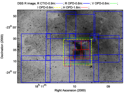
Figure 2.— Position of the polarimetric mapped fields superposed to a R-band DSS image of Sh 2-29. Each line color and style is related to different spectral bands and telescopes used, as indicated by the caption at the top.

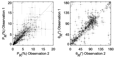
Figure 3.— Comparison between polarization degrees (left) and polarization angles (right) for Sh 2-29 objects observed more than once at R-band observations, due to superposition of adjacent frames (see Figure 2). Equality lines (dashed) are included in order to facilitate the comparison.

Table 1 Polarimetric data set for Sh 2-29 at optical (V, R, I) and near-IR bands (H)

ID	$\alpha_{2000}(^{hms})$	$\delta_{2000}(\arcdeg\arcmin\arcsec)$	$P_{V}(\%)$	$\theta_{V}(^{\circ})$	$P_{R}(\%)$	$\theta_{R}(^{\circ})$	$P_{I}(\%)$	$\theta_{I}(^{\circ})$	$P_{H}(\%)$	$\theta_{H}(^{\circ})$
1	18 8 35.44	-24 17 34.4	$*$	$*$	$7.51(3.27)$	$14.6(11.4)$	$*$	$*$	$*$	$*$
2	18 8 35.59	-23 52 5.6	$*$	$*$	$3.62(1.38)$	$86.5(10.2)$	$*$	$*$	$*$	$*$
3	18 8 35.64	-24 10 42.9	$*$	$*$	$16.84(4.54)$	$18.5(7.5)$	$*$	$*$	$*$	$*$
1116	18 9 31.42	-24 02 43.3	$5.77(0.40)$	$29.6(3.2)$	$4.80(0.23)$	$22.0(1.5)$	$3.78(0.59)$	$38.5(4.8)$	$*$	$*$
1188	18 9 33.54	-24 07 18.5	$*$	$*$	$*$	$*$	$*$	$*$	$2.28(0.34)$	$175.0(7.3)$
1295	18 9 35.73	-24 08 07.2	$5.59(1.21)$	$3.6(6.6)$	$3.15(0.69)$	$177.9(6.2)$	$3.32(0.42)$	$173.4(4.0)$	$1.35(0.29)$	$178.1(8.5)$
1399	18 9 37.56	-24 08 15.0	$3.64(0.48)$	$172.1(4.5)$	$3.82(0.21)$	$173.9(1.7)$	$3.54(0.13)$	$169.8(2.0)$	$0.96(0.07)$	$163.0(6.3)$
1502	18 9 39.04	-24 02 16.2	$4.69(1.35)$	$47.9(8.3)$	$4.42(0.92)$	$35.8(5.9)$	$4.25(0.71)$	$31.9(5.1)$	$1.33(0.50)$	$35.1(11.7)$
1751	18 9 42.67	-24 10 41.5	$1.52(0.59)$	$101.5(10.7)$	$0.61(0.32)$	$120.5(13.4)$	$0.87(0.31)$	$90.5(9.9)$	$*$	$*$

Figure 2 shows a R-band DSS image of Sh 2-29, used to indicate the mapped fields from each band and telescope, as detailed in the caption above the image. The BDS2003 2 embedded cluster is at the center, surrounded by the arc-shaped shell. R-band observations provide a large spatial coverage, consisting of 11 fields obtained with the OPD-0.6 m telescope (solid blue line), summed to an additional field focused on the central cluster observed at the CTIO-0.9 m telescope (dashed blue line). V and I bands were obtained for only one field centered on the embedded cluster, using the OPD-0.6 m telescope (dot-dashed lines, respectively green and yellow). Near-IR H band observations using the OPD-1.6 m telescope are shown by the 5 smaller rectangular areas (solid red line), covering the central cluster, as well as some nearby structures. Slight variations in the H-band field size is a consequence of small imperfections in the jittering process.

Figure 2 shows that several superposition areas exist between adjacent fields, particularly for R-band observations. Such property was used to test the data reproducibility, since within these areas the same stars were observed more than once. In some cases, particularly near the central cluster, stars were independently observed up to 5 times. Hence, $P_{R}(1)\times P_{R}(2)$ and $\theta_{R}(1)\times\theta_{R}(2)$ diagrams were built, as shown in Figure 3, by comparing each observation pair related to the same object. Taking into account the error bars, a good correlation is noted in most cases, generating a well-defined band of points around the equality line. A larger disparity is present toward some objects in the polarization angle comparison, mainly related to cases where polarization degree is low, and therefore $\theta$ is not a well-defined quantity. To each repeated observation, the chosen value to be used on the following analysis was the one with larger $P/\sigma_{P}$ (best quality). Although there is no evidence of the existence of intrinsic polarization (as will be discussed in the next Sections), some differences may not be explained from the analysis of the error bars, what perhaps could be related to an intrinsic time-dependent variation of polarization, which is common to be found specially toward young stars with circunstellar disks (see for example, Pereyra et al., 2009).

In order to demonstrate the content and organization of the polarization values set, a portion of the collected data is shown in Table 1. The total number of detected stars in at least one of the four observed spectral bands sums up to 5254 objects.

Complementing the information provided by the polarimetric sample, a dust extinction map ($A_{V}$) was constructed from 2MASS point source catalog (PSC) JHK photometry data and the NICEST algorithm (Lombardi, 2009). Sources with infrared excess, mostly candidate young stellar objects (YSO’s) with dusty envelopes were removed from the catalog, as they have intrinsically red colors. The NICEST method estimates extinction by comparing the colors of background stars reddened by dust, with the intrinsic colors of extinction-free sources from a nearby control field. The map is constructed by spatial smoothing of individual extinction measurements, using the weighted mean of values as a function of position. NICEST combines Gaussian weighting and a bias correction for the decrease of the number of sources available as a function of extinction. We used a Gaussian width of 60 arc-second (equivalent to a beam resolution for the map), and Nyquist sampling. Contours exhibited in Figure 1 were derived from this map.

4. Results

4.1. Linear polarization mapping in the R optical band

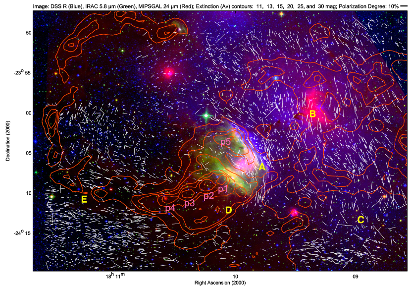
Figure 4.— R band polarimetric mapping of Sh 2-29. The combined image is composed by the R band (DSS, blue), as well as by the 5.8 and 24$\,\mu$m bands from Spitzer (respectively green and red). The size of each vector is proportional to $P$ (a $P=10\%$ vector is shown at the upper right). Labels from A to E are used to highlight some of the main features inferred from the polarization vectors’ orientation pattern, as discussed in Section 5.1. Indicators p1 to p5 show the location of dense cloud structures around the central cavity, presenting peak extinction values between $A_{V}=20$ and $A_{V}>35$ (see Section 5.6).

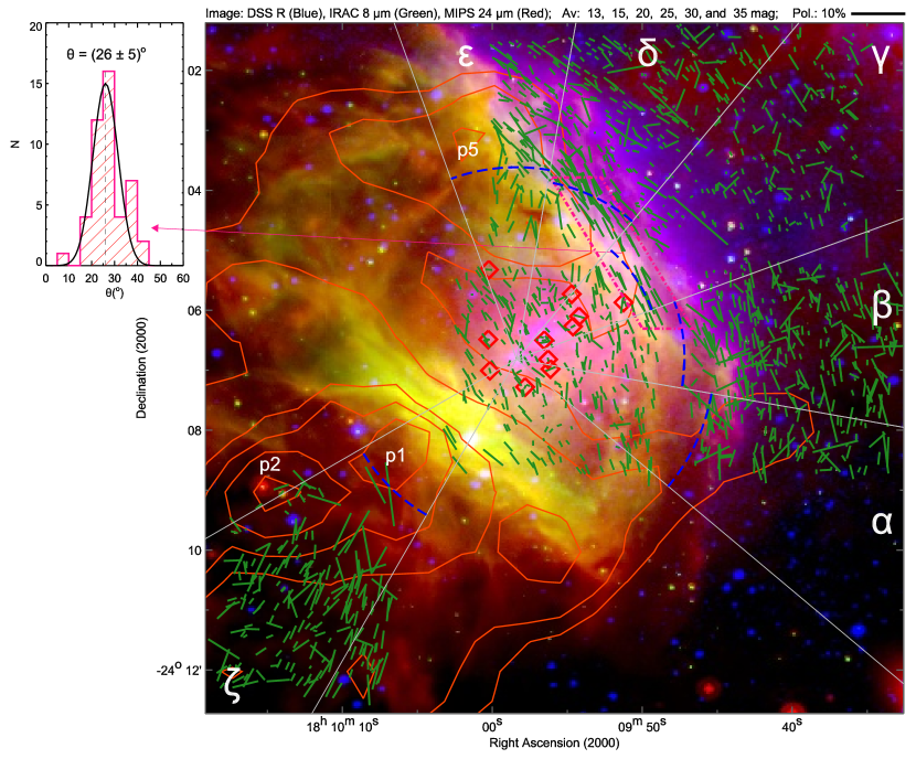
Figure 5.— Near-IR (H band) polarimetric mapping toward the Sh 2-29 central interstellar cavity. A RGB combined image of this area is used, corresponding to the R-DSS band (blue), as well as the $8$ and $24~{}\mu$m bands from Spitzer (respectively green and red). The radial strips labeled from $\alpha$ to $\zeta$ are used to study polarization degree as a function of radius (Section 5.5), with the blue dashed lines indicating the positions were a rise in polarization occur. Red diamonds mark the positions of those stars presenting H$\alpha$ emission (Ogura et al., 2002) that were detected in the polarimetric survey. The dot-dashed pink polygon indicates the area which was used to apply the Chandrasekhar-Fermi method (see Section 5.8). The polarization angle histogram shown at the left is used in this same analysis in order to derive the angle dispersion within this area.

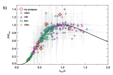
Figure 6.— Fits of the Serkowski relation for several objects toward Sh 2-29.          Part a shows three examples of $P(\%)\times\lambda^{-1}     (\mu$m${}^{-1})$ diagrams, where each fitted values of $P_{max}$ and          $\lambda_{max}$ are listed at the top, as well as the total-to-selective          extinction $R$. A $P/P_{max}\times\lambda_{max}/\lambda$ diagram          is shown in part b, which has been built with all available polarimetric          data for the 87 objects from the sample. The Serkowski curve is represented by          the dark solid line, while different colored symbols denote the sets of spectral          bands used at each fitting (as detailed by the caption inside the diagram).          Data points marked by red diamonds indicate polarization values for 3 stars with          H$\alpha$ emission (Ogura et al., 2002). Part c exhibits a histogram of $\theta_{R}-\theta_{H}$ to show the correlation in polarization angles between bands R and H for all objects used in the Serkowski fits with detections in these two bands.              

Figure 4 shows the R-band linear polarization vectors superposed to a combined false-color image of R (DSS, blue), 5.8 and 24$\,\mu$m bands (Spitzer, respectively green and red). Polarization degree $P$ is linearly related to the size of each vector.

Assuming that the interstellar dust grains’ orientation is predominantly determined by the typical alignment mechanisms (Davis & Greenstein, 1951), then the polarization direction is parallel to the sky-projected component of magnetic field lines. However, it is important to emphasize that the observed polarization values are not a result of a simple line-of-sight additive effect, and actually depend on the distance to each source and on the variations of the interstellar medium properties along its direction. For instance, if a star is located behind the star-forming region, its polarimetric parameters are represented by a combined effect of the Sh 2-29 interstellar medium together with the foreground dust component. Such properties will be further explored in Section 5.2.

Furthermore, it is possible that young stellar objects contribute with an intrinsic polarization component, which may arise, for example, if these sources present circumstellar disks with an asymmetrical sky projection. This effect would probably be mostly important closer to regions with greater star-forming activity, such as the interior of the central interstellar cavity, where the embedded cluster BDS2003 2 is located. Several young stars with H$\alpha$ emission are found in this area, as represented by the red diamonds on Figure 1 (Ogura et al., 2002). Since most of these objects are normally too obscured, only a few were detected on the optical observations. Besides, the global orientation pattern of polarization vectors exhibit a high local correlation within specific areas. Such effect may only be explained due to the predominance of the polarization effect due to the interstellar medium. Therefore, the importance of a possible intrinsic polarimetric component is probably not statistically significant in this analysis (however, it may be important on the analysis of the H band polarimetric properties near the central cavity, as will be discussed in Section 4.2).

4.2. Linear polarization mapping in the H band

Figure 5 shows the H-band polarimetric mapping, which covers a smaller area focused on the central cavity and nearby surroundings. The image consists of a RGB combination of the R-DSS (blue) and Spitzer’s $8$ and $24~{}\mu$m bands (respectively green and red). It is evident that within the H-band survey area, a much larger number of stars were detected, as compared to the same area at the optical observations, since interstellar extinction is lower at near-IR bands.

At the near-IR observations, several stars with H$\alpha$ emission were detected, as shown by red diamonds in Figure 5 (Ogura et al., 2002). Therefore, these are potential targets that may show some intrinsic polarization component. In order to test this hypothesis, we compare its polarimetric parameters (degree and angle) with nearby objects that do not show H$\alpha$ emission. Any significant diverging trend could be and indication that some level of intrinsic polarization arising from the circunstellar disk is in fact superposed to the interstellar component. This comparison shows that objects with H$\alpha$ emission have polarization degree values roughly distributed between $P_{H}=0.5\%$ and $2.3\%$, which is similar to the levels shown by other nearby stars located inside the central cavity. Likewise, it is also difficult to distinguish any significant difference in the distribution of polarization angles for stars with and without H$\alpha$ emission. These evidences suggest that, similarly to the R-band survey, it is not possible to infer any intrinsic polarimetric component that could be statistically significant, therefore interfering with the analysis of interstellar magnetic field lines. As will be shown in Section 4.3, an analysis of linear polarization in multiple spectral bands may provide further indications to support this hypothesis.

4.3. Wavelength dependence of polarization and fits of the Serkowski relation

In order to study interstellar grains’ features toward the Hii region’s central cavity and close surroundings, we have used the multi-band polarimetric data to compute fits of the Serkowski relation (Serkowski et al., 1975), which may be expressed as:

$$P_{\lambda}=P_{max}\exp{\left[-K\ln^{2}{\left(\frac{\lambda_{max}}{\lambda}\right)}\right]}$$ (2)

Such empirical equation represents the dependence of polarization degree $P$ with wavelength $\lambda$, where $P_{max}$ and $\lambda_{max}$ respectively denote the maximum polarization level and the wavelength where this maximum value is reached. The $K$ parameter typically assumes the value $1.15$ (Serkowski et al., 1975; Codina-Landaberry & Magalhaes, 1976).

By combining the polarimetric data in all available spectral bands (V, R, I, and H), we have chosen objects observed at least in three different wavelengths, and applied the fitting method proposed by Coyne (1974), which basically consists of a linearization of Equation 2. We have also restricted the sample to those objects presenting $P/\sigma_{P}>3$ on all available bands, resulting in 87 stars satisfying these criteria. Three examples of fittings of the Serkowski relation ($P\times\lambda^{-1}$ diagrams) are shown in Figure 6a, together with the respective values of $P_{max}$ and $\lambda_{max}$.

In each case, we have also computed the parameter $R$, which represents the total-to-selective extinction ratio ($R=A_{V}/E_{B-V}$) with values shown in Figure 6a for each example. $R$ is directly linked to $\lambda_{max}$ through the relation $R=(5.6\pm 0.3)\lambda_{max}$ (Serkowski et al., 1975; Whittet & van Breda, 1978), and therefore may be easily obtained from this method.

Figure 6b shows a $P/P_{max}\times\lambda_{max}/\lambda$ diagram, where we have used the polarization degree values at each available spectral band for all 87 objects. Different symbols and colors are related to the sets of spectral bands used at each fitting, as detailed by the caption inside the diagram. Among these objects, 3 present H$\alpha$ emission (red diamonds, Ogura et al., 2002), and 82 are available at the 2MASS catalogue (this correlation will be essential to the analysis shown in Section 5.9).

Data points clearly define a thick band around the Serkowski curve in this diagram. Although some scattering is obviously present, this is probably mainly a consequence of the natural data uncertainties, as may be inferred by the analysis of the error bars. Greater scattering and uncertainty levels occur for higher $\lambda_{max}/\lambda$ values, and therefore this is mainly related to the V and R spectral bands. This is an expected trend, since many of these stars are highly embedded, resulting in lower signal-to-noise ratios at higher frequency detections, as compared to the near-IR band.

By studying the data distribution for the 3 stars with H$\alpha$ emission (Figure 6b), we notice that although some points present a significant scattering when compared to the position of the curve, it is probably generated by the natural scattering also detected for other stars, mainly in the V and R bands data. Therefore, we may conclude that although some intrinsic polarization level may exist for objects with indications of the presence of circumstellar disks, such contribution is probably too low when compared to the prevailing dichroic effect due to magnetically aligned interstellar dust grains.

Figure 6c shows a histogram of $\theta_{R}-\theta_{H}$ which have been constructed from all stars used in the Serkowski fits that presented detections in both R and H bands. Although there is a large concentration of stars with $\theta_{R}-\theta_{H}$ close to zero (indicating a correlation between these two quantities), there is clearly a spread in this distribution, ranging from $-15\arcdeg$ to $\sim 25\arcdeg$. Also, the peak of this distribution seems slightly displaced toward positive values. These features are expected, since a polarized stellar light beam that traverses different interstellar layers, presenting different grain properties and alignment conditions, should be affected by a rotation effect of the polarization angle with respect to wavelength (Gehrels & Silvester, 1965; Coyne, 1974; Messinger et al., 1997). Given the filamentary nature of this central area, and also the fact that there is a foreground polarizing dust component, the distribution’s spread and displacement may be explained by the rotation effect.

5. Analysis and discussion

5.1. Qualitative analysis of magnetic field lines’ morphology

Several conspicuous features related to the general morphology of magnetic field lines may be immediately noticed through an overview analysis of the polarimetric mappings from Figures 4 and 5. In this Section, these properties are discussed in detail, and some hypothesis related to the generation and evolution of these structures are raised. Labels from A to E are shown in Figure 4 to highlight the positions of these characteristics.

Initially, the most notable feature, indicated by A, corresponds to a large arc-shaped orientation of polarization vectors, which are curved around the central cavity, mostly following the same morphology of the extended H$\alpha$ emission seen in the R-band image. The similarity in shape between the magnetic field lines and this interstellar structure (which is related to the ionized gas) suggests a strong correlation among these features. Moreover, such arc-shaped characteristic, enfolding and following the cavity’s borders, is consistent with a possible expansion of this central volume, affecting the properties of the surrounding regions.

Some properties of the cavity’s expansion may be inferred by studying its morphological features mainly through Spitzer’s mid-IR images, particularly the $5.8\,\mu$m band (green color in Figure 4). The cavity is defined by two thick interstellar shells – or slabs – which are approximately parallel to each other, and surround the stellar cluster located at its center. One shell is located toward the Northwest of the cluster (above it and to the right), while the other is located toward the Southeastern direction (below and to the left). By studying the $A_{V}$ contours, one may notice that above these shells, interstellar extinction is higher ($A_{V}\gtrsim 13$ mag, therefore indicating a higher dust and gas density), as compared to the nearby areas. These evidences suggest that due to the expansion of the ionized gas inside the cavity, interstellar material has been swept out from the center (where $A_{V}$ is lower), being driven toward its borders, and consequently pilling up in this region. Since magnetic fields are probably coupled to the interstellar gas, its shape may have been affected during this process, possibly resulting in a pile-up effect of field lines along the cavity’s borders. Such effect will be further analysed in Section 5.5.

The same alignment of polarization vectors with the cavity’s Northwest border is observed at the H-band map (Figure 5, especially toward the dot-dashed pink polygon). Furthermore, by analysing the vector’s sizes, we notice that polarization degree toward such border area seems higher on average, as compared to vectors located inside the cavity. Such feature seems to indicate a spatial dependence of polarization degree, especially when the region is analysed from inside-out (this property is further explored in detail in Section 5.5). Apart from these trending features, the H-band mapping shows a large dispersion of polarization vectors’ orientation (the same dispersion is observed toward the central cavity at the optical mapping). Given the large number of complex sub-structures (such as ionizing fronts, interstellar filaments, etc.), it is probably an effect of the line-of-sight superposition of these features toward this smaller-scale area.

A subtle arc-shaped distortion of the field is also noticed around the region labelled B in Figure 4, although not so evident as in region A. This region surrounds the massive star HD165921, as well as an associated 24 $\mu$m emission feature, visible as a red spot. The presence of this star (the most massive object in the Hii region) is probably strongly affecting its nearby environment, ionizing, sweeping and heating the material, consequently causing a distortion of magnetic field lines. In general, between regions A and B polarization vector’s morphology is consistent with a flux of magnetic field lines being compressed due to the expansion of two fronts at opposite sides (the central cavity and the region around HD165921). Besides, around the entire area surrounding region B, polarization vectors seem very well ordered and uniformly oriented. If Sh 2-29 is regarded as a large shell in expansion around HD165921 and its associated ionized region (as discussed in Section 2, according to the interpretation by Yamaguchi et al., 1999), then a higher uniformity of magnetic field lines is indeed expected along its expanding borders, as shown for example by simulations of expanding Hii regions (Arthur et al., 2011). Such hypothesis will be further explored in Section 5.4.

At region C, an abrupt change in vectors’ mean direction occurs by comparing the area toward its North (vectors vertically oriented) and its South (vectors horizontally distributed). This region indicates the Southern border of the Hii region, since the H$\alpha$ extended emission from ionized gas (seen in blue at the image) gradually diminishes from North to South around this area. Therefore, the predominantly horizontal polarimetric orientation below region C is probably related to magnetic field lines outside the Hii region. Around region D, a Southern portion of the Simeis 188 dark cloud is present (as revealed by the extinction contours), resulting in a significantly lower number of polarimetric optical detections.

At the region around E, the cloud extends to the East in a large arc shape which is curved toward the North, defining the Hii region’s left border. Above E region, the vectors follow the shape of the cloud, roughly bending toward the North. However, a large dispersion of polarization vectors exist around this area, suggesting that the alignment of magnetic field lines is not very prominent (as occurs around A and B, for example). Even though, the fact that field lines above E in general follow the cloud’s morphology (differing from the horizontal trend outside the Hii region, below E) suggest that the formation of this cloud has somehow shaped the morphology of magnetic fields, probably by dragging its lines along the same process.

5.2. Analysis of the foreground R-band polarization component

Before carrying on with the analysis of magnetic field lines’ morphology (using the R-band map), it is important to evaluate the foreground polarization component, which is intrinsically present for all background objects. In order to apply quantitative methods of analysis, it is necessary to remove such contribution (see Section 5.3), since it may cause a direct influence on the vectors’ orientation.

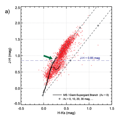
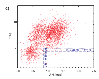
Figure 7.— Correlation between $P_{R}$ and 2MASS near-IR data for Sh 2-29. Graph (a) is a color-color diagram ($J-H\times H-Ks$) using only stars with R-band polarimetric detections. Dashed gray lines represent the reddening band (Rieke & Lebofsky, 1985), while circular dots above these lines denote positions for $A_{V}=10,20,30$ mag, etc. Part (b) shows a $J-H$ histogram highlighting the narrowing of points at $J-H=0.85$ (green arrow). Diagram (c) represents the relation between $P_{R}$ and $(J-H)$, using the same data set.

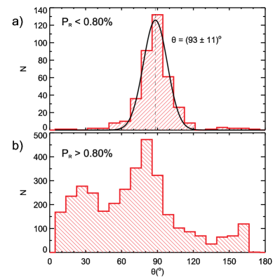
Figure 8.— Distributions of R-band polarimetric angles, considering stars with $P_{R}<0.80\%$ (diagram a) and $P_{R}>0.80\%$ (diagram b).

In order to study the extinction properties of the observed stars, we begin by correlating the R-band polarimetric data with objects from the 2MASS catalog. Figure 7a shows a $(J-H)\times(H-Ks)$ color-color diagram, made only from stars with R band polarimetric detections. In this diagram, dark solid lines correspond to the un-reddened main sequence, giants and super-giants loci (Koornneef, 1983; Carpenter, 2001), while gray dashed lines represent the reddening band (assuming the standard reddening law, Rieke & Lebofsky, 1985).

A large stellar group is located around the un-reddened main sequence and giants area, therefore presenting lower extinction values. Moreover, several objects are spread along the reddening band, indicating stars with higher extinction values (and therefore have a higher probability of being located within or behind the star-forming region). These two groups may be roughly separated by noting a subtle narrowing of the points’ distribution, as indicated by the green arrow, at approximately $J-H=0.85$ mag. Such narrowing may be clearly verified by examining the $J-H$ histogram in Figure 7b, therefore providing an approximate distinction between the lower and higher extinction stars.

Figure 7c shows a $P_{R}\times(J-H)$ diagram, built with the same data set used in Figure 7a. This type of diagram is useful to highlight the imperfect correlation between linear polarization and interstellar extinction, an expected trend for general polarization measurements (Serkowski et al., 1975). It is obvious that for higher $(J-H)$ values (and therefore $A_{V}$), polarization degree average values are also higher. We also notice that for $J-H\gtrsim 0.85$ mag, the majority of points follow a very clear trend: there is a minimum polarization value of approximately $0.80\%$. Stars near this lower limit are reddened enough to present $J-H>0.85$ suggesting that their location is close to or within the molecular cloud. However, their low polarization values indicates that they are probably not significantly affected by the polarizing effects due to the cloud itself, and therefore are possibly located close to its near edge. Thereafter, such minimum value must correspond to the foreground component, which is an integrated result of all interstellar material between the molecular cloud and the observer. This means that all higher extinction objects (located within or behind the Sh 2-29 region), present this minimum polarization component value. Based on the points’ dispersion near this minimum value, we estimate a foreground polarization degree of $P_{R}=0.80\pm 0.25\%$.

In order to estimate the foreground polarization angle we use the entire R-band data set to build polarization angle distributions for stars with $P_{R}<0.80\%$ (Figure 8a) and $P_{R}>0.80\%$ (Figure 8b). This method allows the comparison of polarization angles between stars averagely located in the foreground with objects from the background. The first distribution shows $\theta_{R}$ values sharply concentrated around $\approx 93\arcdeg$. In fact, considering the relatively small area where the R-band data is distributed – approximately $35^{\prime}\times 45^{\prime}$ – such trend is consistent with the fact that the foreground component should not show large angle variations. On the other hand, the distribution of polarization angles for $P_{R}>0.80\%$, shows a much larger dispersion, which is indeed expected based on the analysis of the large angle variations from the mapping of Figure 4. Notice that in Figure 8b there is a peak around $\theta\sim 30\arcdeg$ that is consistent with the polarization pattern around region B (Figure 4), therefore clearly related to the Hii region. Concluding, there is a clear distinction of polarization orientation between the foreground population and stars affected by more distant interstellar structures. A Gaussian fit applied to the distribution from Figure 8a results in a foreground polarization angle of $\theta_{R}=93\pm 11\arcdeg$.

The foreground polarization values toward Sh 2-29 ($P_{R}$ and $\theta_{R}$) may be compared with the foreground polarization values in the direction of the Lagoon Nebula, as estimated by McCall et al. (1990). As discussed in Section 2, this is a nearby star-forming region, located only $1.6\arcdeg$ from Sh 2-29. Its foreground polarization values are $P=0.81\pm 0.15$% and $\theta=79\pm 9\arcdeg$ at the V optical band, which are consistent with our estimates, giving further support to the idea that within relatively close areas in the sky, it is not expected that this component should suffer large variations.

By converting the foreground polarization angle to galactic coordinates, we find $\theta_{gal}=154\arcdeg$. Analysing large-scale Galactic polarimetric mappings (Mathewson & Ford, 1970; Heiles, 2000; Santos et al., 2011), we notice that around $(l,b)\approx(7\arcdeg,-2\arcdeg)$, there is a mixture of several distinct alignments, including an orientation which is consistent with $\theta_{gal}=154\arcdeg$. Toward such line-of-sight several sub-structures from the local interstellar medium near the Sun are known to exist (especially those related to the Loop I superbubble’s shells), and therefore could be responsible for the foreground polarimetric direction (see for example, Santos et al., 2011).

5.3. Stokes parameters’ removal of the R-band foreground component

The R-band foreground polarimetric contribution may be removed in order to allow the application of quantitative methods which are dependent on polarization angles (see Section 5.4). Since a great variety of different orientations are present in the Sh 2-29 polarimetric map, the existence of such contribution causes a polarization increase or decrease, depending on whether the vector lies parallel or perpendicular to the foreground polarization component.

When a light beam traverses different interstellar layers, although linear polarization may not be considered an additive effect, its associated Stokes parameters $Q$ and $U$ may be successively summed. Therefore, we may consider that toward a specific object, the observed Stokes parameters ($Q,U$) are composed by a foreground component ($Q_{f},U_{f}$), added to a second component which traces Sh 2-29’s magnetic field lines ($Q_{\mathrm{Sh2-29}},U_{\mathrm{Sh2-29}}$):

$$Q=Q_{f}+Q_{\mathrm{Sh2-29}}\ \ \ \ \mathrm{and}\ \ \ \ U=U_{f}+U_{\mathrm{Sh2-29}}$$ (3)

The parameters associated to the foreground component were determined by $Q_{f}=P\cos{2\theta}$ and $U_{f}=P\sin{2\theta}$, where $P$ and $\theta$ values are those estimated in Section 5.2. By subtracting these factors from each ($Q,U$) pair, $Q_{\mathrm{Sh2-29}}$ and $U_{\mathrm{Sh2-29}}$ were obtained, and used to compute the corrected $P_{\mathrm{Sh2-29}}$ and $\theta_{\mathrm{Sh2-29}}$ values through Equation 1.

The corrected polarization mapping is shown in Figure 9a, where vectors are superposed to a combined image of the R-band (DSS, blue) and $5.8\,\mu$m band (Spitzer, green). The visual effect is very small, as compared to Figure 4, since the foreground polarization degree is generally small ($0.8\%$) relative to the typical polarization values ($\sim 2-10\%$). However, such correction is important, since the slight modification in individual polarization angles may result in significant changes in the statistical analysis of the turbulence of magnetic fields (presented in the next Section).

5.4. Turbulence of magnetic fields from the optical polarization mapping

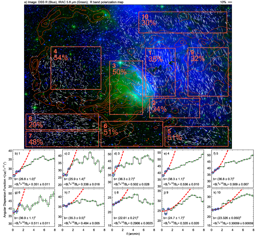
Figure 9.— Statistical analysis of the Angle Dispersion Function (ADF) to different areas located toward the R-band studied region of Sh 2-29. Map (a) shows R-band polarimetric vectors, corrected from the foreground component, superposed to a R/$5.8\,\mu$m-band combined image (blue/green). Different rectangular areas (1 to 10) are shown over this image, and ADF diagrams (b) to (k) are respectively related to these areas. Computed values of $\langle B_{t}^{2}\rangle^{1/2}/B_{0}$ for every area are shown both inside each ADF diagram, and also inside each respective area from the polarimetric map.

As discussed in Section 5.1, several hypothesis related to the interaction between the interstellar structures and magnetic fields toward Sh 2-29 were formulated, based solely on a qualitative analysis of the linear polarization mappings. Several of these hypothesis may be tested on a quantitative manner, by studying the magnetic field’s turbulence degree throughout the region, i.e., the ratio between its turbulent ($B_{t}$) and uniform component ($B_{0}$).

The method is based on a statistical analysis proposed by Hildebrand et al. (2009). It consists mainly in computing the second-order Structure Function of polarization angles ($\langle\Delta\Phi^{2}(l)\rangle$, hereafter SF). This function may be described as the average value of the squared difference in polarization angles between two points separated by a distance $l$ (see Equation (5) given by Falceta-Gonçalves et al., 2008). Its square root is defined as the Angular Dispersion Function ($\mathrm{ADF}=\sqrt{\mathrm{SF}}$), and may be used to evaluate how polarization angles (and therefore magnetic field lines), are spatially correlated, as a function of the separation $l$. According to Hildebrand et al. (2009), if the turbulent and uniform fields are respectively associated to correlation lengths $\delta$ and $d$, then the method is valid within the range $\delta<l\ll d$. Moreover, the SF may be represented as an addition of a few statistically independent contributions:

$$\langle\Delta\Phi^{2}(l)\rangle\simeq b^{2}+m^{2}l^{2}+\sigma^{2}(l)$$ (4)

The first term is related to a constant turbulent contribution $b$, the second term represents a smooth rise in the SF as the separation $l$ increases (this behaviour is considered to be linear in the ADF, with its slope denoted by $m$), and the third term is a roughly constant factor due to measurements uncertainties ($\sigma(l)$). After removing the last term from each of the SF’s bins, it is possible to compute the ADF and determine the $b$ factor (the intercept of the ADF at $l=0$) through a simple linear fit using Equation 4. This factor is the essential target for this method, since it is directly related to the turbulence degree by:

$$\frac{\langle B_{t}^{2}\rangle^{1/2}}{B_{0}}=\frac{b}{\sqrt{2-b^{2}}}$$ (5)

In order to apply this procedure to the R-band polarimetric data toward Sh 2-29 (corrected by the foreground component) and study the variations of $\langle B_{t}^{2}\rangle^{1/2}/B_{0}$ throughout the region, different rectangular areas have been selected, labeled from 1 to 10 in Figure 9a. The selections were based on the data distribution and on the different images’ features observed toward each area. Also, the region’s sizes were chosen such as to provide a sufficient number of vectors needed to perform the statistical analysis (the typical number is between $200$ and $300$ although some regions present fewer or more vectors). The procedure described above have been applied to polarimetric vectors inside each area. The respective ADF diagrams are shown in Figures from 9b to 9k, together with the fitted values for the $b$ parameter and the magnetic turbulence degree $\langle B_{t}^{2}\rangle^{1/2}/B_{0}$ (these are also shown inside each area of Figure 9a). In each case, $0.5^{\prime}$-sized bins were used, and only the first three points were considered in the linear fit to Equation 4, in order to guarantee the validity of the condition $l\ll d$.

Regions 1, 2, 9 and 10 coincide with the area that supposedly have been affected by the Hii region’s expansion, and also where a higher intensity of the H$\alpha$ extended emission is noted (blue color in the composed image). Particularly, region 1 corresponds to the area located among two possible fronts expanding toward each other (the first due to the central cavity, and the second related to the massive object HD165921), as discussed in Section 5.1. Comparing magnetic turbulence degree values within these areas, with more external regions (such as 5, 6 and 7), considerably lower levels are found (roughly from 30 to 35%). This trend is consistent with the compression and consequent uniformity of magnetic field lines, due to the expansion of the Hii region’s surrounding shell, lending support to the previously detailed hypothesis.

Areas 5, 6 and 7 denote the Hii region’s external regions, below its Southern rim. This entire area is dominated by horizontally oriented vectors, differing significantly from the pattern observed inside the ionized volume. Furthermore, $\langle B_{t}^{2}\rangle^{1/2}/B_{0}$ values also diverge significantly, showing higher levels (between 48 and 51%), suggesting that this area probably have not been affected by any ordering effect and/or dragging of magnetic field lines.

A particularly interesting trend may be noticed by the comparison between regions 7 and 8: although these areas are spatially close and apparently both unaffected by the Hii region’s expansion, magnetic turbulence degree toward region 8 (closer to the dark cloud’s arc-shaped rim) is much lower ($29\%$) relative to region 7 ($48\%$) located immediately to the South. This may suggest that closer to the cloud, the field lines’ orientation pattern is more uniform and less random. Besides, in Section 5.1 we have suggested that the same process which have generated the arc-shaped cloud’s morphology, may also have induced the orientation of magnetic field lines parallel to the cloud (region E in Figure 4). The correlation of these information points toward a possible explanation for the difference in magnetic turbulence degree between areas 7 and 8: the process that distorted the cloud into an arc-shape was followed by a compression and pile-up effect of magnetic field lines behind the expanding cloud area, consequently creating a more uniform pattern closer to the cloud. Therefore, such interpretation is consistent with the fact that $\langle B_{t}^{2}\rangle^{1/2}/B_{0}$ decreases nearer to the cloud around this region.

During the evolution of an Hii region, it is expected that more evolved areas cease to expand after several million years, due to the balance between internal and external pressures, leading to an equilibrium state (Spitzer, 1978). Therefore, it is not possible to assert that the expansion which has possibly distorted the cloud, together with the interstellar magnetic field lines, still exists. If Sh 2-29’s eastern area is more evolved, this could explain the fact that toward area 4, a high magnetic turbulence degree is detected (54%): if field lines have previously been ordered due to expansion and compression effects, the evolution of the system could have led to a subsequent interaction with interstellar gas’ inherent turbulence. Therefore, such interaction may have been responsible for rearranging and distorting its organized pattern, consequently increasing its random magnetic component.

Other hypothesis that could explain the relatively higher turbulence degree towards area 4 is related to its distance from the region’s ionizing objects: the nearer known massive object that could ionize this region is HD166192, of spectral type B2ii. It may be noted that the H$\alpha$ extended emission is relatively less intense toward this area, which could indicate a lower ionization level. Therefore, it is probable that the flux of ultraviolet ionizing photons from this star have a lower radius range, if compared for example, to HD165921 (spectral type O7v+O9v), which is likely responsible for the ionization and expansion effects around areas 1, 2, 9 and 10. Consequently, it is also possible that the expansion effect toward area 4 is not very intense, not causing a great disturbance in the surrounding clouds, and therefore, not capable of producing a sufficiently pronounced ordering of magnetic field lines.

Toward the central cavity (area 3), a high level of magnetic turbulence is also detected (50%). Since many interstellar sub-structures and filamentary clouds exist toward this area, it is quite possible that this value is a result of the superposition of differently oriented field lines related to these small scale features.

5.5. Pilling up of magnetic field lines around the cluster’s cavity

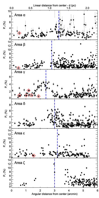
Figure 10.— H-band polarization degree ($P_{H}$) as a function of the distance $r$ from the center of Sh 2-29’s interstellar cavity. Each diagram is correlated to one of the radial sections labelled as $\alpha$ to $\zeta$ in Figure 5. The horizontal axis from the bottom corresponds to the angular radial distance (in arcmin), while the top axis represents the linear distance (in parsecs, assuming a distance of $d=1.3$ kpc). The blue dashed vertical lines indicate the positions where we notice an increase in $P_{H}$ mean value (or at least to some few objects), as compared to the levels closer to the center. Red diamonds indicate stars with H$\alpha$ emission.

In order to study de behaviour of polarization degree as a function of the radius toward the central cavity, we have chosen radial sections in Figure 5 (labelled $\alpha$ to $\zeta$), originating from the cavity’s center, where the BDS2003 2 cluster is located. These areas were selected based on the data distribution, providing at least $100$ vectors were found inside each sector. $P_{H}\times r$ diagrams have been built to each section, as shown in Figure 10.

Typically, $P_{H}$ levels between $0.5$ and $3\%$ are found inside the cavity. By analysing the $P_{H}\times r$ diagrams, we notice that for every radial section, a rise of the typical $P_{H}$ value occurs at a certain radius, as indicated by the blue dashed lines. Such increase is more or less prominent, depending on the studied section. For example, regions $\gamma$ and $\delta$ show a sharp rise in $P_{H}$ (assuming values between $\approx 2$ and $7\%$) at approximately $r=2-3$ arcmin. On the other hand, regions $\alpha$, $\beta$, $\epsilon$ and $\zeta$ show a less marked rise in $P_{H}$, with some sparse points assuming higher values, as compared to levels found inside the cavity.

In Figure 5 we show the same approximate positions where the polarization elevation occurs (blue dashed lines for each section), indicating a good general correlation with the location of the cavity’s edge. We may interpret this effect as a result of the pilling up of magnetic field lines at these borders, which were dragged outwards due to the volume’s expansion from the action of young massive stars and ionized gas inside the region. The result of this pile-up effect is a higher intensity of the magnetic field at this area, which probably causes a direct influence on the efficiency of the dominant grain alignment mechanism. Therefore, a higher value of the magnetic field is probably responsible for a better alignment of interstellar dust grains at the cavity’s borders, leading to higher detected values of linear polarization.

5.6. Interstellar extinction peaks around the central cavity

Examining the Sh 2-29 extinction map we notice the existence of some highly obscured interstellar extinction peaks located around the cavity’s edge. These objects are labelled as p1 to p5 in Figure 4, and present peak extinction values between $A_{V}=20$ and $37$ mag. Structures p1 to p4 are approximately aligned within the dark cloud, below and to the left of the central cavity (all presenting peak $A_{V}>28$ mag), while p5 (peak $A_{V}=20.9$ mag) is located toward the North, coinciding with the cavity’s northern edge (see Figures 4 and 5).

Table 2 Properties of dense interstellar structures around Sh 2-29’s central cavity

Core ID	$\alpha_{2000}(^{hms})$	$\delta_{2000}(\arcdeg\arcmin\arcsec)$	Ang. Diam. (′)	Diam. (pc)	Peak $A_{V}$	Mean $A_{V}$	$N_{\mathrm{H_{2}}}$ (cm-2)	$n_{\mathrm{H_{2}}}$ (cm-3)	$M_{\mathrm{H_{2}}}$ (M⊙)
p1	18 10 15.1	-24 09 01.3	$\sim$1.50	0.57	34.2	30.1	$2.8\times 10^{22}$	$1.6\times 10^{4}$	77
p2	18 10 06.4	-24 08 28.4	$\sim$1.75	0.66	36.6	32.5	$3.1\times 10^{22}$	$1.5\times 10^{4}$	112
p3	18 10 23.6	-24 10 01.4	$\sim$1.50	0.57	33.5	30.5	$2.9\times 10^{22}$	$1.6\times 10^{4}$	77
p4	18 10 32.7	-24 10 59.6	$\sim$1.25	0.47	28.4	26.7	$2.5\times 10^{22}$	$1.7\times 10^{4}$	46
p5	18 10 01.6	-24 03 02.7	$\sim$2.00	0.75	20.9	17.5	$1.6\times 10^{22}$	$0.7\times 10^{4}$	76

Based on each peak’s extinction profile, we have estimated several physical properties, which are shown in Table 2. An approximate angular diameter is computed (in arcmin) and subsequently converted to linear diameter (in parsecs), by assuming a distance of $1.3$ kpc (Fich & Blitz, 1984). In order to estimate the average molecular hydrogen density ($n_{\mathrm{H_{2}}}$) and mass ($M_{\mathrm{H_{2}}}$), we begin by computing the mean $A_{V}$ within each peak’s projected area. We assume that the gas-to-dust ratio between hydrogen’s total column density (i.e., neutral and molecular, $N_{\mathrm{H(total)}}=N_{\mathrm{HI+H_{2}}}$), and color excess $E(B-V)$ is given by de $5.8\times 10^{21}$ particles cm^-2 mag^-1 (Jenkins & Savage, 1974; Bohlin et al., 1978; Pineda et al., 2010). Assuming further that all hydrogen content within such high-density volume is constituted by its molecular form, then $N_{\mathrm{H(total)}}=2N_{\mathrm{H_{2}}}$, and therefore $N_{\mathrm{H_{2}}}/E(B-V)=2.9\times 10^{21}$ cm^-2 mag^-1. In order to convert between $E(B-V)$ and $A_{V}$, we assume the typical interstellar law $A_{V}=3.1E(B-V)$. Finally, the relation between molecular gas and extinction is $N_{\mathrm{H_{2}}}/A_{V}=9.4\times 10^{20}$ cm^-2 mag^-1. By means of such relation, we have computed the $\mathrm{H_{2}}$ column density toward each extinction peak, based on the $A_{V}$ mean values shown in Table 2. Assuming that the structure’s projected diameter is similar to the line-of-sight dimension, the mean molecular hydrogen density ($n_{\mathrm{H_{2}}}$) was estimated. Also, considering approximately spherical shapes, the $\mathrm{H_{2}}$ mass could be deduced.

Molecular hydrogen density and mass values are respectively in the range $0.7$ – $1.7\times 10^{4}$ cm^-3 and $46$ – $112$ solar masses. Furthermore, its dimensions vary between $\sim 0.40$ and $0.80$ pc. Such estimates suggest that these fragmentations could represent dense interstellar clumps, as compared for example, with studies from Williams & Blitz (1998) and Román-Zúñiga et al. (2012). Therefore, each of these individual structures may be considered as important targets for future small scale and high resolution observations. However, such values should be regarded as rough estimates, in view of the number of assumptions used in the computations. For instance, variations in the total-to-selective extinction ratio are frequent inside molecular clouds and Hii regions, typically varying between $R=2.5$ and $5.0$ (see Section 5.9). Furthermore, variations in distance and in the molecular hydrogen fraction could cause large changes in the physical values. Also, the extinction map has a limited resolution, so that other gas and dust tracers at radio and sub-millimeter spectral bands could be used for a better characterization of these targets. Therefore, we estimate that variations of approximately $\approx 50\%$ could occur for the $n_{\mathrm{H_{2}}}$ and $M_{\mathrm{H_{2}}}$ values.

It is quite remarkable, however, that by comparing the position of these dense interstellar fragmentations, with Spitzer’s $24\,\mu$m emission (the red image component in Figures 4 and 5), we notice the existence of some point-like sources, with a significant flux in such spectral band. These sources are particularly close to peaks p2 and p4, respectively at positions $(\alpha,\delta)_{J2000}=(18^{\mathrm{h}}10^{\mathrm{m}}15.4^{\mathrm{s}},-24\arcdeg 08^{\prime}55.7^{\prime\prime})$ and $(\alpha,\delta)_{J2000}=(18^{\mathrm{h}}10^{\mathrm{m}}34.8^{\mathrm{s}},-24\arcdeg 10^{\prime}43.1^{\prime\prime})$. Other mid-IR point-like sources may also be identified by the inspection of the regions close to dense extinction peaks p1-p4. The emission feature from this spectral region is usually linked to young stellar objects, presenting thermal dust emission due to the circumstellar disk. Therefore, this scenario is consistent with the presence of proto-stellar objects ongoing formation inside the dense interstellar fragmentations.

5.7. The relation among the interstellar extinction peaks and the magnetic field lines’ morphology

A comparison between the dense extinction peak’s properties and the magnetic field lines (as revealed by Figure 5) also leads to interesting results. Among those interstellar structures indicated in Table 2, p5 is the one with lower peak $A_{V}$ and $n_{\mathrm{H_{2}}}$. This extinction peak is located toward the cavity’s northern edge, where field lines seem to pile-up parallel to the border, therefore roughly perpendicular to the interstellar material expansion direction. Besides, p5 coincides with the extended structure detected at $450$ and $850\,\mu$m bands by Morgan et al. (2008) (which is also coincident with IRAS 18068-2405 source). As described in Section 2, such feature was studied by Urquhart et al. (2009), who concluded that mid-IR point-like sources still does not exist within this area, and that the interstellar density enhancement has probably been induced due to some external event.

These hypothesis are very consistent with our interpretation that the central interstellar cavity is expanding, consequently leading to a pilling up of interstellar material along its borders, and therefore probably being responsible for the formation of p5 during this same process. Moreover, it is possible that the expansion direction perpendicular to the field lines may have contributed to detain the advancing ionization front, hindering a larger pilling up of interstellar material in this area (as compared to peaks p1-p4, for example), due to the higher magnetic pressure. Other possibility, however, is that the differences in density between the interstellar extinction peaks is otherwise due to simple non-uniformities in the initial surrounding medium, before being affected by the effects of the cavity’s expansion.

In contrast, toward fragmentations p1-p4 the polarization vectors’ orientation suggest that field lines are rather perpendicular to the cavity’s borders, and therefore are probably roughly parallel to its expanding flux. We may infer that such configuration possibly facilitates the expansion of the cavity’s southeastern rim, leading toward the dark cloud’s densest portion (where peaks p1-p4 are located). Such expansion may have been responsible for generating instabilities and fragmentations, which led to the interstellar material contraction and collapse into highly obscured structures (peak $A_{V}>30$ mag). Several models describe the triggered collapse of interstellar clumps and cores due to externally induced shock waves, as discussed for example, by Boss (1995), Hennebelle et al. (2003, 2004), Whitworth (2007) and André et al. (2009). As previously suggested, such collapse possibly resulted in the formation of the next generation of proto-stars with significant mid-IR emission.

5.8. Magnetic field strength at the line compression zone

In Section 5.5 we have suggested that the increase in polarization degree detected toward the central cavity’s borders is a consequence of the larger magnetic field intensity, due to the pilling up effect. If this idea is correct, a direct estimate of the magnetic field strength in this area should provide a higher value, as compared to typical levels observed at the diffuse interstellar medium.

A relatively simple procedure to estimate $B$ is the Chandrasekhar-Fermi (CF) method (Chandrasekhar & Fermi, 1953), which is based on the idea that magnetic field irregularities are a natural consequence of turbulent motions from the interstellar medium. Such relation is obvious, since field lines are coupled to the interstellar gas, providing that at least a small ionization fraction exists (Spitzer, 1978; Heiles & Crutcher, 2005). These irregularities will produce a larger dispersion in the orientation of polarization vectors. However, for a larger $B$ value, field lines’ shape is less susceptible to the turbulence effects. Therefore, a lower polarization angle dispersion results in a higher $B$ level, and vice-versa. The sky-projected field strength may be expressed as (Crutcher et al., 2004; Heiles & Crutcher, 2005):

$$B =Q\sqrt{4\pi\rho}\;\frac{\delta V}{\delta\theta}\;$$ (6)

$$\approx 9.3\biggl{(}\frac{n_{\mathrm{H_{2}}}}{\mathrm{cm}^{-3}}\biggr{)}^{1/2}\biggl{(}\frac{\Delta V}{\mathrm{kms^{-1}}}\biggr{)}\biggl{(}\frac{\delta\theta}{1\arcdeg}\biggr{)}^{-1}\;\mu\mathrm{G}$$

where $\delta V$ is the velocity dispersion ($\Delta V=\sqrt{8\ln{2}}\;\delta V$ is the FWHM corresponding to the spectral line used in this computation), $\rho$ is the gas density (where we assume the predominance of molecular hydrogen), and $\delta\theta$ is the polarization angle dispersion. The parameter Q, which has the approximate value of $0.5$ (according to molecular cloud simulations, Ostriker et al., 2001), corresponds to a correction and calibration of the CF relation, in order to account for several factors, such as line-of-sight field fluctuations, velocity perturbations anisotropies, gas density inhomogeneities, etc (Zweibel, 1990; Myers & Goodman, 1991). Nevertheless, according to the same simulations, this method is valid only for low dispersion values ($\delta\theta<25\arcdeg$).

The CF method was applied to the cavity’s border area indicated by dot-dashed pink polygon in Figure 5. The $P\times r$ diagrams toward this region (Figure 10, sections $\gamma$ and $\delta$), show a sharply increase in polarization degree. The polarization angle histogram shown at the top left of Figure 5 exhibit a distribution highly concentrated around $\theta=26\arcdeg$, with a dispersion of only $\delta\theta=5\arcdeg$ (computed through the Gaussian fit). It is important to account for the measurement uncertainties, which contribute with a fraction of this dispersion value. The mean value of polarization angle uncertainty for vectors inside the polygon, is $\langle\sigma_{\theta}\rangle=4.1\arcdeg$. The corrected angle dispersion value ($\delta\theta^{\prime}$), to be used in Equation 6, may be obtained considering that $\delta\theta=\sqrt{(\delta\theta^{\prime})^{2}+\langle\sigma_{\theta}\rangle^{2}}$, providing $\delta\theta^{\prime}=2.9\arcdeg$.

The velocity dispersion values toward dense fragmentation p5 (which is separated from the selected area by only $\approx 3$ arcmin) was obtained by Urquhart et al. (2009) through the study of ¹²CO and ¹³CO lines, providing respectively $\Delta V=2.0$ and $1.9$ km s^-1. We have used the average value, i.e., $\Delta V=1.95$ km s^-1. A careful inspection of the extinction levels within the polygon indicate a mean value of $A_{V}\approx 13$ mag. Using the same gas-to-dust relation discussed in Section 5.6, and assuming an angular diameter of about $3^{\prime}$ (corresponding to an interstellar structure at the cavity’s border with length of $\approx 1$ pc), we find $n_{\mathrm{H_{2}}}\approx 4.0\times 10^{3}$ cm^-3.

Applying these quantities to Equation 6 provides $B\approx 400\,\mu$G, which is a much larger value as compared to the magnetic field strength in the diffuse interstellar medium ($\sim 6\,\mu$G, Beck, 2001; Heiles & Crutcher, 2005). This evidence corroborates the previous hypothesis that a higher $B$ level should arise within this area, as a consequence of the cavity’s expansion, leading to a pilling up effect. Magnetic field estimates toward star-forming regions through the CF method, as well as Zeeman effect analyses, show that high $B$ values are typical in such environments. On one hand, values ranging from $80\,\mu$G (for example, toward the pre-stellar core L 183, Crutcher et al., 2004) up to about $50000-80000\,\mu$G have already been found (see the study of W 3, Orion KL, W49N, and S140 regions, conducted by Fiebig & Guesten, 1989). On the other hand, much lower values have been found toward the magnetically dominated Pipe Nebula (varying between $17$ and $65\,\mu$G, depending on the position along the cloud, as discussed by Alves et al., 2008; Franco et al., 2010), which shows several starless and quiescent cores. Perhaps this could indicate magnetic field differences between high and low mass star-forming regions, although more studies are necessary.

It is important to point out that this $B$ computation is highly approximate, due to its dependence on several factors which may only be roughly estimated. However, it is still a valid approach that allows to evaluate its order of magnitude. The low precision is mainly a consequence of the uncertainty related to the interstellar density, since this property is dependent on various assumptions, such as: the typical value of $R=3.09$ related to the extinction law; the presence of other species besides molecular hydrogen, such as atomic and ionized hydrogen; the estimate of the cloud line-of-sight thickness, etc.

5.9. The distribution of the ratio of total-to-selective extinction values toward Sh 2-29

In Section 4.3 we have shown how the multi-band polarimetric analysis could be used to derive the $R$ values to 87 objects from our sample. As discussed before, this parameter is highly influenced by the interstellar grain size distribution, and therefore may be used as a probe of the dust conditions surrounding the central cavity. The typical grain size at the diffuse interstellar medium corresponds to $\langle a\rangle\approx 0.15\,\mu$m, which represents $R\approx 3.09$. Considering a diffuse cloud with a standard grain size distribution composed by particles larger and smaller than the mean value, the $R$ value is proportional to the ratio between the number of larger and smaller grains. Therefore, an increase in the relative number of larger grains will generate a higher $R$ value, and vice-versa.

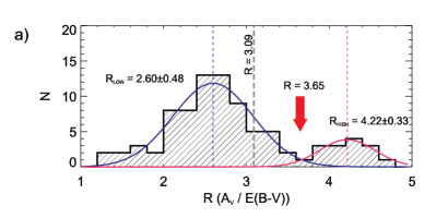
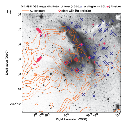
Figure 11.— Diagram (a) shows the distribution of $R$ values, using the results of the 87 Serkowski fits computed from the multi-band polarimetric sample. Solid curves represent Gaussian fits to the higher (red line) and lower (blue line) $R$ distribution trends, respectively centered at $2.60\pm 0.48$ and $4.22\pm 0.33$ (the uncertainties correspond to the 1-$\sigma$ dispersion). Diagram (b) shows the spatial distribution of objects with $R<3.65$ ($\times$ blue symbol) and $R>3.65$ ($+$ pink symbol). Red diamonds indicate the position of 3 stars with H$\alpha$ emission (Ogura et al., 2002).

In order to study the distribution of $R$ values toward the Sh 2-29 central area, we have built the histogram shown in Figure 11a. A concentration peaked around the standard value ($R=3.09$) would be expected for the diffuse interstellar medium (Larson & Whittet, 2005, Fig. 7). Instead, it is clear from this diagram that two opposite trends dominate the distribution, both diverging considerably from the standard value. The most prominent concentration corresponds to a pronounced peak around $R_{low}=2.60\pm 0.48$ (as indicated by the blue Gaussian fit), i.e., showing a predominance of $R$ values lower than $3.09$. The second trend is related to higher values, peaked around $R_{high}=4.22\pm 0.33$ (as shown by the red Gaussian fit). It is less marked as compared to the first trend, suggesting that $R$ values toward the central cavity are predominantly lower than $3.09$, although some few lines-of-sight indicate higher values.

In order to study the different properties between both trending populations of $R$ values, we notice from Figure 11a that these distributions are well separated, in a sense that there is not much superposition between them. In fact, we may define the value $R=3.65$ (indicated by the red arrow) as a convenient limiting value roughly distinguishing both distributions.

Figure 11b shows the spatial distribution of $R$ values larger ($+$ symbol, pink color) and smaller than $3.65$ ($\times$ symbol, blue color), toward the central cavity. There is obviously a mixture of directions with $R>3.65$ and $R<3.65$, with a clear predominance of smaller values, specially toward the ionization front. It is notable, however, that examining the regions to the left of the central cavity (where the denser extension of the dark cloud is located), 4 among 5 of the objects with $R$ values present $R>3.65$ (as indicated by the upper and lower pink arrows). To the only star with $R<3.65$ in this area (located immediately below the upper arrow), the computed value is $R=3.2$, which is still above the standard $3.09$ value. Therefore, there is a weak evidence that regions with higher $R$ values suffered lower impact from the massive central stars, being located near the edges of the cloud’s denser portions, therefore probably shielded and protected from the action of intense shock fronts. Obviously, several stars with $R>3.65$ may also be observed toward the central cavity and surrounding its prominent arc-shaped ionization front. However, it is important to point out that its individual projected distances are not known, and therefore, these objects may also be located at the cloud’s nearer edge tracing the neutral instead of ionized gas.

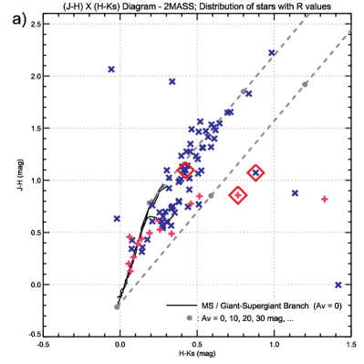
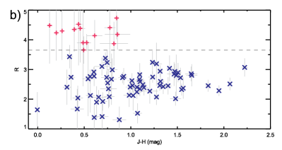
Figure 12.— (a) Color-color diagram ($J-H\times H-Ks$) for objects with $R$ values, based on 2MASS magnitudes. Symbols and colors follow the same criteria used in Figure 11b. The positions of the un-reddened main sequence, giants and super-giants, as well as the reddening band, are similar to Figure 7a. (b) $R\times J-H$ diagram, using the same stars from part (a). The horizontal dashed line corresponds to $R=3.65$, as defined in order to separate between the higher and lower $R$ values.

A further analysis may be carried out, by correlating the $R$ values with 2MASS near-IR photometric data. Figure 12a shows the color-color diagram ($J-H\times H-Ks$) with different symbols and colors for stars with $R<3.65$ and $R>3.65$, as in Figure 11b. Objects with $R<3.65$ are predominantly distributed along the reddening band, presenting a wide variety of extinction levels (between $0$ and $\approx 15$ mag). On the other hand, most of the objects with $R>3.65$ are concentrated near the un-reddened main sequence locus, with an exception of only two objects showing color excess in the near-IR (located to the right of the reddening band). Such trends are even more evident in the $R\times J-H$ diagram shown in Figure 12b. Notice that for objects with $R>3.65$, there is a limiting $J-H$ value of roughly $0.9$ mag, suggesting a lower reddening levels toward these stars. This is a further evidence that objects with higher $R$ values, even those which are located in the direction of the arc-shaped ionization front, are possibly located at the edges of the cloud encompassing the star-forming region, where $A_{V}$ levels are lower.

5.10. Interpreting the anomalous $R$ values toward Sh 2-29: processing of interstellar dust grains

Several processes in the interstellar medium may cause alterations in the grain sizes, leading to anomalous $R$ values, which may be higher (Vrba & Rydgren, 1985; Whittet et al., 2001) or lower (Larson et al., 1996; Szomoru & Guhathakurta, 1999; Larson & Whittet, 2005) than the standard value, depending on the environment’s local physical conditions (Jones, 2004; Mazzei & Barbaro, 2008).

Normally, larger $R$ values may be found within dense clouds, where coagulation effects due to grain-grain collisions are common. However, coagulation will only be sufficiently efficient on low-velocity collisions (between $0.001$ and $0.02$ km s^-1), which implies on relatively isolated clouds, generally unaffected or shielded from turbulence or shock waves (Chokshi et al., 1993; Jones et al., 1996; Hirashita, 2012; Köhler et al., 2012). Other process that could lead to higher $R$ values is the grain evaporation (or sublimation) due to the incidence of highly energetic photons (extreme ultraviolet and $\gamma$-rays), since smaller grains are most sensitive to this kind of grain destruction mechanism (Guhathakurta & Draine, 1989).

On the other hand, smaller $R$ values are usually related to regions affected by shock waves, where sputtering effects (due to the collision between grains and atoms/ions) tend to favor the destruction of larger grains (Mathis et al., 1977; Jones et al., 1996). Other possibility is that the turbulence generated by shock waves lead to a higher mean grain velocity, which results in fragmentation effects: it is know that for velocities higher than $\approx 1$ km s^-1, coagulation effects will be replaced by fragmentation of dust particles, which constitutes an efficient mechanism to convert grains from large into smaller sizes (Borkowski & Dwek, 1995; Jones et al., 1996).

McCall et al. (1990) found an anomalous value of $R=4.6\pm 0.3$ toward the Lagoon region, which is spatially close to Sh 2-29. According to their interpretation, stars from the sample used in that case are most likely related to neutral gas, and therefore are probably located at the Hii region’s edges. It was proposed that the higher $R$ value is probably due to a combined effect of coagulation and evaporation by energetic photons which traverses the cloud’s dense and neutral external shells. In the case of the coagulation hypothesis the anomaly would be the result of grain growth effects due to the presence of a relic component of the original dense cloud which gave birth to the star-forming region.

In view of the several physical effects which may alter the average grain sizes, the existence of two opposite grain populations toward Sh 2-29 may now be interpreted. In Section 5.9 we have shown that the higher $R$ component seems to be related to peripheral locations (near the outskirts of the dense cloud), as well as to lower extinction values. Therefore, these sites are possibly remnants of the initial dense cloud which originated the star-forming region, probably still weakly disturbed by star formation effects, such as shock waves due to massive stars. At such relic cloud component, coagulation effects probably dominated the previous dense environment, leading to larger $R$ values. Therefore, this population of large grains is probably still preserved in this environment which is seemingly protected from the grain destruction mechanisms. This effect is very similar to the one detected toward the Lagoon nearby region, corroborating our hypothesis. Some stars with higher $R$ values could actually be regarded as foreground objects, although it would not be consistent with the fact the foreground component is probably represented by a standard extinction law, since it corresponds to the diffuse interstellar medium.

On the other hand, the lower $R$ component is predominant inside the central cavity and toward the arc-shaped H$\alpha$ feature, where there is certainly a large influence of expanding ionization fronts, turbulence and stellar winds from young massive stars. This environment is consistent with sputtering and grain fragmentation effects, which promotes an efficient mechanism that converts larger into smaller dust particles, leading to lower mean $R$ values.

Concluding, the observation of different grain populations toward a single region from the interstellar medium is remarkable, revealing the evolution process of dust particles. In this case the evidence suggest that the grains’ evolutionary stage surrounding Sh 2-29 corresponds to a gradual conversion from an earlier predominantly larger size component to an environment where smaller size dust particles now prevail. Such processing effects of interstellar dust, observed during the course of the particles’ transformation mechanism, has rarely been detected before within a specific region of the Galaxy, and lends support to the theories of grain evolution.

6. Conclusions

In this work we have used multi-band polarimetric data (V, R, I and H) toward Sh 2-29 in order to study properties from the interstellar magnetic field lines, as well as the size distribution of dust particles. A visual extinction map, together with R-band (DSS) and mid-IR (Spitzer) images were used to reveal several interstellar features. The main results from this analysis are listed below.

1. The most striking feature from Sh 2-29 is an interstellar cavity surrounding an embedded stellar cluster. The analysis of R and H-band polarimetric mappings, together with the visual extinction levels, suggests that this cavity is expanding and dragging both the interstellar material and the magnetic field lines outwards, which pile-up along its arc-shaped borders. This effect probably leads to a higher magnetic field strength of about $400\,\mu$G, as estimated from the Chandrasekhar-Fermi method. Consequently, grain alignment mechanisms are more efficient, resulting in higher levels of polarization degree, as revealed by the study of polarization as a function of radial distance from the center;

2. After correcting the R-band polarization sample from the foreground component, statistical analyses were performed by computing the angular dispersion function, in order to evaluate the magnetic turbulence degree ($\langle B_{t}^{2}\rangle^{1/2}/B_{0}$) toward several areas distributed throughout the Hii region. In a general way, lower turbulence degree values ($30-35\%$) are found toward areas that are probably undergoing an expansion process due to the ionized gas, hence leading to a highly ordered pattern characterizing the compressed field lines. On the other hand, areas unaffected by the expansion, located outside the Hii region toward its South, generally present higher turbulence degree levels ($48-51\%$). An exception occurs toward the eastern portion of the dark cloud, where its arc-shaped extension seems to have compressed field lines located immediately below its southern rim;

3. A group of prominent, dust extinction peaks, were found to exist surrounding the central cavity’s external borders (probably generated due to its expansion), with peak visual extinction values between $20$ and $37$ mag. Estimated levels of molecular hydrogen density and mass are respectively in the ranges of $0.7$ – $1.7\times 10^{4}$ cm^-3 and $46$ – $112$ solar masses, which is compatible with interstellar clumps. Their positions are correlated with point-like sources from Spitzer’s $24\,\mu$m observations, and therefore likely represent new generations of young stars being born within its densest portions, showing sufficient mid-IR emission from a warm circumstellar disk. Interpretation of the magnetic field configuration, correlated with the structures’ density and extinction levels, suggest that the cavity’s expansion may have been hindered (due to magnetic pressure) or facilitated, depending on the relation between the expansion direction and field line orientation;

4. The multi-band polarimetric analysis allowed the study of the total-to-selective extinction distribution, revealing two clearly distinct trends peaked at $R_{low}=2.60\pm 0.48$ and $R_{high}=4.22\pm 0.33$, i.e., both diverging significantly from the standard $3.09$ value. The first trend is predominant, and is probably related to lower mean grain sizes inside the central cavity and surroundings due to intense shock fronts, leading to sputtering and dust fragmentation effects. The second trend is less marked, and is seemingly related to a relic component of the previous dense cloud which gave birth to the star-forming site, where probably coagulation effects resulted in larger mean grain sizes.

Sh 2-29 has been revealed as a very rich Galactic environment, where several interesting aspects of star formation sites may be simultaneously observed: young stars and its interaction with the surrounding environment, disturbance of interstellar magnetic fields, triggered formation of dense clumps, processing of interstellar dust particles, etc. Future studies will involve a near-IR photometric and spectroscopic analysis of the embedded stellar population, which is pending a detailed characterization. Moreover, a complete characterization of the dense fragmentations (with sub-mm and radio wavelengths) could reveal interesting properties of the next young stellar generation.

References

- Altenhoff et al. (1970) Altenhoff, W. J., Downes, D., Goad, L., Maxwell, A., & Rinehart, R. 1970, A&AS, 1, 319
- Alves et al. (2008) Alves, F. O., Franco, G. A. P., & Girart, J. M. 2008, A&A, 486, L13
- André et al. (2009) André, P., Basu, S., & Inutsuka, S. 2009, The formation and evolution of prestellar cores (Cambridge University Press), 254
- Arias et al. (2007) Arias, J. I., Barbá, R. H., & Morrell, N. I. 2007, MNRAS, 374, 1253
- Arthur et al. (2011) Arthur, S. J., Henney, W. J., Mellema, G., de Colle, F., & Vázquez-Semadeni, E. 2011, MNRAS, 414, 1747
- Beck (2001) Beck, R. 2001, Space Sci. Rev., 99, 243
- Bica et al. (2003) Bica, E., Dutra, C. M., Soares, J., & Barbuy, B. 2003, A&A, 404, 223
- Blitz et al. (1982) Blitz, L., Fich, M., & Stark, A. A. 1982, ApJS, 49, 183
- Bohlin et al. (1978) Bohlin, R. C., Savage, B. D., & Drake, J. F. 1978, ApJ, 224, 132
- Borkowski & Dwek (1995) Borkowski, K. J. & Dwek, E. 1995, ApJ, 454, 254
- Boss (1995) Boss, A. P. 1995, ApJ, 439, 224
- Cambrésy et al. (2011) Cambrésy, L., Rho, J., Marshall, D. J., & Reach, W. T. 2011, A&A, 527, A141
- Carpenter (2001) Carpenter, J. M. 2001, AJ, 121, 2851
- Carruthers & Page (1984) Carruthers, G. R. & Page, T. 1984, ApJS, 55, 101
- Chandrasekhar & Fermi (1953) Chandrasekhar, S. & Fermi, E. 1953, ApJ, 118, 113
- Chokshi et al. (1993) Chokshi, A., Tielens, A. G. G. M., & Hollenbach, D. 1993, ApJ, 407, 806
- Codina-Landaberry & Magalhaes (1976) Codina-Landaberry, S. & Magalhaes, A. M. 1976, A&A, 49, 407
- Coyne (1974) Coyne, G. V. 1974, AJ, 79, 565
- Crutcher (2005) Crutcher, R. 2005, in The Magnetized Plasma in Galaxy Evolution, ed. K. T. Chyzy, K. Otmianowska-Mazur, M. Soida, & R.-J. Dettmar , 103–110
- Crutcher et al. (2004) Crutcher, R. M., Nutter, D. J., Ward-Thompson, D., & Kirk, J. M. 2004, ApJ, 600, 279
- Dahm et al. (2012) Dahm, S. E., Herbig, G. H., & Bowler, B. P. 2012, AJ, 143, 3
- Davis & Greenstein (1951) Davis, Jr., L. & Greenstein, J. L. 1951, ApJ, 114, 206
- Falceta-Gonçalves et al. (2008) Falceta-Gonçalves, D., Lazarian, A., & Kowal, G. 2008, ApJ, 679, 537
- Fich & Blitz (1984) Fich, M. & Blitz, L. 1984, ApJ, 279, 125
- Fich et al. (1990) Fich, M., Dahl, G. P., & Treffers, R. R. 1990, AJ, 99, 622
- Fiebig & Guesten (1989) Fiebig, D. & Guesten, R. 1989, A&A, 214, 333
- Fosalba et al. (2002) Fosalba, P., Lazarian, A., Prunet, S., & Tauber, J. A. 2002, ApJ, 564, 762
- Franco et al. (2010) Franco, G. A. P., Alves, F. O., & Girart, J. M. 2010, ApJ, 723, 146
- Gehrels & Silvester (1965) Gehrels, T. & Silvester, A. B. 1965, AJ, 70, 579
- Georgelin et al. (1973) Georgelin, Y. M., Georgelin, Y. P., & Roux, S. 1973, A&A, 25, 337
- Girart et al. (2009) Girart, J. M., Beltrán, M. T., Zhang, Q., Rao, R., & Estalella, R. 2009, Science, 324, 1408
- Guhathakurta & Draine (1989) Guhathakurta, P. & Draine, B. T. 1989, ApJ, 345, 230
- Heiles (2000) Heiles, C. 2000, AJ, 119, 923
- Heiles & Crutcher (2005) Heiles, C. & Crutcher, R. 2005, in Lecture Notes in Physics, Berlin Springer Verlag, Vol. 664, Cosmic Magnetic Fields, ed. R. Wielebinski & R. Beck, 137
- Heitsch et al. (2004) Heitsch, F., Zweibel, E. G., Slyz, A. D., & Devriendt, J. E. G. 2004, ApJ, 603, 165
- Hennebelle et al. (2004) Hennebelle, P., Whitworth, A. P., Cha, S.-H., & Goodwin, S. P. 2004, MNRAS, 348, 687
- Hennebelle et al. (2003) Hennebelle, P., Whitworth, A. P., Gladwin, P. P., & André, P. 2003, MNRAS, 340, 870
- Herbig (1957) Herbig, G. H. 1957, ApJ, 125, 654
- Hildebrand et al. (2009) Hildebrand, R. H., Kirby, L., Dotson, J. L., Houde, M., & Vaillancourt, J. E. 2009, ApJ, 696, 567
- Hirashita (2012) Hirashita, H. 2012, MNRAS, 422, 1263
- Jenkins & Savage (1974) Jenkins, E. B. & Savage, B. D. 1974, ApJ, 187, 243
- Jones (2004) Jones, A. P. 2004, in Astronomical Society of the Pacific Conference Series, Vol. 309, Astrophysics of Dust, ed. A. N. Witt, G. C. Clayton, & B. T. Draine, 347
- Jones et al. (1996) Jones, A. P., Tielens, A. G. G. M., & Hollenbach, D. J. 1996, ApJ, 469, 740
- Kandori et al. (2007) Kandori, R., Tamura, M., Kusakabe, N., et al. 2007, PASJ, 59, 487
- Köhler et al. (2012) Köhler, M., Stepnik, B., Jones, A. P., et al. 2012, A&A, 548, A61
- Koornneef (1983) Koornneef, J. 1983, A&A, 128, 84
- Krumholz et al. (2007) Krumholz, M. R., Stone, J. M., & Gardiner, T. A. 2007, ApJ, 671, 518
- Kusakabe et al. (2008) Kusakabe, N., Tamura, M., Kandori, R., et al. 2008, AJ, 136, 621
- Larson & Whittet (2005) Larson, K. A. & Whittet, D. C. B. 2005, ApJ, 623, 897
- Larson et al. (1996) Larson, K. A., Whittet, D. C. B., & Hough, J. H. 1996, ApJ, 472, 755
- Leão et al. (2012) Leão, M. R. M., de Gouveia Dal Pino, E. M., Santos-Lima, R., & Lazarian, A. 2012, ArXiv e-prints
- Lizano & Shu (1989) Lizano, S. & Shu, F. H. 1989, ApJ, 342, 834
- Lombardi (2009) Lombardi, M. 2009, A&A, 493, 735
- Mathewson & Ford (1970) Mathewson, D. S. & Ford, V. L. 1970, MmRAS, 74, 139
- Mathis et al. (1977) Mathis, J. S., Rumpl, W., & Nordsieck, K. H. 1977, ApJ, 217, 425
- Matthews et al. (2002) Matthews, B. C., Fiege, J. D., & Moriarty-Schieven, G. 2002, ApJ, 569, 304
- Mazzei & Barbaro (2008) Mazzei, P. & Barbaro, G. 2008, MNRAS, 390, 706
- McCall et al. (1990) McCall, M. L., Richer, M. G., & Visvanathan, N. 1990, ApJ, 357, 502
- McKee & Ostriker (2007) McKee, C. F. & Ostriker, E. C. 2007, ARA&A, 45, 565
- Messinger et al. (1997) Messinger, D. W., Whittet, D. C. B., & Roberge, W. G. 1997, ApJ, 487, 314
- Mestel & Spitzer (1956) Mestel, L. & Spitzer, Jr., L. 1956, MNRAS, 116, 503
- Morgan et al. (2008) Morgan, L. K., Thompson, M. A., Urquhart, J. S., & White, G. J. 2008, A&A, 477, 557
- Mouschovias & Paleologou (1981) Mouschovias, T. C. & Paleologou, E. V. 1981, ApJ, 246, 48
- Myers & Goodman (1991) Myers, P. C. & Goodman, A. A. 1991, ApJ, 373, 509
- Nakano (1979) Nakano, T. 1979, PASJ, 31, 697
- Novak et al. (1997) Novak, G., Dotson, J. L., Dowell, C. D., et al. 1997, ApJ, 487, 320
- Novak et al. (2000) Novak, G., Dotson, J. L., Dowell, C. D., et al. 2000, ApJ, 529, 241
- Novak et al. (1989) Novak, G., Gonatas, D. P., Hildebrand, R. H., Platt, S. R., & Dragovan, M. 1989, ApJ, 345, 802
- Ogura et al. (2002) Ogura, K., Sugitani, K., & Pickles, A. 2002, AJ, 123, 2597
- Oka et al. (1999) Oka, T., Kawai, N., Naito, T., et al. 1999, ApJ, 526, 764
- Ostriker et al. (2001) Ostriker, E. C., Stone, J. M., & Gammie, C. F. 2001, ApJ, 546, 980
- Padoan et al. (2004) Padoan, P., Jimenez, R., Juvela, M., & Nordlund, Å. 2004, ApJ, 604, L49
- Pereyra (2000) Pereyra, A. 2000, Ph.D. Thesis, Univ. São Paulo (Brazil)
- Pereyra et al. (2009) Pereyra, A., Girart, J. M., Magalhães, A. M., Rodrigues, C. V., & de Araújo, F. X. 2009, A&A, 501, 595
- Pineda et al. (2010) Pineda, J. L., Goldsmith, P. F., Chapman, N., et al. 2010, ApJ, 721, 686
- Rho et al. (2008) Rho, J., Lefloch, B., Reach, W. T., & Cernicharo, J. 2008, M20: Star Formation in a Young HII Region (Reipurth, B.), 509
- Rieke & Lebofsky (1985) Rieke, G. H. & Lebofsky, M. J. 1985, ApJ, 288, 618
- Román-Zúñiga et al. (2012) Román-Zúñiga, C. G., Frau, P., Girart, J. M., & Alves, J. F. 2012, ApJ, 747, 149
- Santos et al. (2011) Santos, F. P., Corradi, W., & Reis, W. 2011, ApJ, 728, 104
- Santos et al. (2012) Santos, F. P., Roman-Lopes, A., & Franco, G. A. P. 2012, ApJ, 751, 138
- Serkowski et al. (1975) Serkowski, K., Mathewson, D. L., & Ford, V. L. 1975, ApJ, 196, 261
- Sharpless (1959) Sharpless, S. 1959, ApJS, 4, 257
- Shu et al. (1987) Shu, F. H., Adams, F. C., & Lizano, S. 1987, ARA&A, 25, 23
- Spitzer (1978) Spitzer, L. 1978, Physical processes in the interstellar medium (New York Wiley-Interscience, 1978. 333 p.)
- Szomoru & Guhathakurta (1999) Szomoru, A. & Guhathakurta, P. 1999, AJ, 117, 2226
- Tang et al. (2009) Tang, Y.-W., Ho, P. T. P., Girart, J. M., et al. 2009, ApJ, 695, 1399
- Tapia (1988) Tapia, S. 1988, Preprints of the Steward Observatory, No. 831
- Tody (1986) Tody, D. 1986, Proc. SPIE, 627, 733
- Turnshek et al. (1990) Turnshek, D. A., Bohlin, R. C., Williamson, R. L., et al. 1990, AJ, 99, 1243
- Urquhart et al. (2009) Urquhart, J. S., Morgan, L. K., & Thompson, M. A. 2009, A&A, 497, 789
- Vogt & Moffat (1975) Vogt, N. & Moffat, A. F. J. 1975, A&A, 45, 405
- Vrba & Rydgren (1985) Vrba, F. J. & Rydgren, A. E. 1985, AJ, 90, 1490
- Wardle & Kronberg (1974) Wardle, J. F. C. & Kronberg, P. P. 1974, ApJ, 194, 249
- Whittet et al. (2001) Whittet, D. C. B., Gerakines, P. A., Hough, J. H., & Shenoy, S. S. 2001, ApJ, 547, 872
- Whittet & van Breda (1978) Whittet, D. C. B. & van Breda, I. G. 1978, A&A, 66, 57
- Whitworth (2007) Whitworth, A. P. 2007, in IAU Symposium, Vol. 237, IAU Symposium, ed. B. G. Elmegreen & J. Palous, 251–257
- Wilking et al. (1980) Wilking, B. A., Lebofsky, M. J., Kemp, J. C., Martin, P. G., & Rieke, G. H. 1980, ApJ, 235, 905
- Wilking et al. (1982) Wilking, B. A., Lebofsky, M. J., & Rieke, G. H. 1982, AJ, 87, 695
- Williams & Blitz (1998) Williams, J. P. & Blitz, L. 1998, ApJ, 494, 657
- Yamaguchi et al. (1999) Yamaguchi, R., Saito, H., Mizuno, N., et al. 1999, PASJ, 51, 791
- Zweibel (1990) Zweibel, E. G. 1990, ApJ, 362, 545