Calibration of semi-analytic models of galaxy formation using Particle Swarm Optimization

Abstract

We present a fast and accurate method to select an optimal set of parameters in semi-analytic models of galaxy formation and evolution (SAMs). Our approach compares the results of a model against a set of observables applying a stochastic technique called Particle Swarm Optimization (PSO), a self-learning algorithm for localizing regions of maximum likelihood in multidimensional spaces that outperforms traditional sampling methods in terms of computational cost. We apply the PSO technique to the SAG semi-analytic model combined with merger trees extracted from a standard $\Lambda$CDM N-body simulation. The calibration is performed using a combination of observed galaxy properties as constraints, including the local stellar mass function and the black hole to bulge mass relation. We test the ability of the PSO algorithm to find the best set of free parameters of the model by comparing the results with those obtained using a MCMC exploration. Both methods find the same maximum likelihood region, however the PSO method requires one order of magnitude less evaluations. This new approach allows a fast estimation of the best-fitting parameter set in multidimensional spaces, providing a practical tool to test the consequences of including other astrophysical processes in SAMs.

1. Introduction

The combination of numerical methods and computational resources provides one of the best tools to study the origin and evolution of structures in the Universe. The Lambda Cold Dark Matter ($\Lambda$CDM) scenario for the growth of dark matter (DM) structures has been extensively studied using numerical N-body simulations, which follow the evolution of such structures from shortly after decoupling to the present-day over a large dynamical range (Springel et al., 2005; Boylan-Kolchin et al., 2009; Klypin et al., 2011; Angulo et al., 2012).

Studying the evolution of baryonic matter is more complex due to the highly non-linear effects of gas, making it impossible (with the current state-of-the-art) to perform a fully self-consistent numerical simulation that resolves all the scales relevant to the physics of galaxy formation in a large volume. In addition, physical processes in the sub-grid scale, such as the star-formation process and different feedback mechanisms are still poorly understood due to their intrinsic complexity. This is why semi-analytic models of galaxy formation (SAMs) play a fundamental role, since they can produce large samples of galaxies at a low computational cost which can be used to study properties such as star formation, luminosity, colors and chemical evolution by following the evolution of baryons in a simplified way (Baugh, 2006; Benson, 2010; Silk & Mamon, 2012; Frenk & White, 2012).

A downside of using SAMs is that they depend on a large number of free parameters which are included in the implementations of the different physical processes modeled; these parameters are usually calibrated by choosing a set of observables that the simulated galaxies are expected to reproduce. Kampakoglou et al. (2008) and Henriques et al. (2009) introduced the Monte Carlo Markov Chains (MCMC) technique to carry out a statistical exploration of the multidimensional parameter space of a SAM. Since this technique is well known, MCMC quickly became a popular tool for calibrating the free parameters of SAMs, using as observational constraints not only $z=0$ data (Henriques et al., 2009; Henriques & Thomas, 2010; Lu et al., 2011, 2012) but also observed or inferred properties at higher redshifts (Mutch et al., 2013b, a; Henriques et al., 2013, 2014).

More refined Bayesian techniques for determining the value of the free parameters in SAMs were introduced by Bower et al. (2010) with the Gaussian model emulator technique (ME) (see e.g. Kennedy & O’Hagan 2001), an approach based in building a statistical predictor for the results from a given model based on a limited set of model runs. The ME technique was also implemented by Gómez et al. (2012, 2014) to study the impact of formation histories on the final satellite population of Milky Way-sized galaxies.

The increasing complexity of SAMs motivate the search for computationally more effective and fast methods to perform calibrations. In this work we apply for the first time another machine learning inspired sampling method, called Particle Swarm Optimization (PSO, Kennedy & Eberhart 1995) to select the optimal set of parameters for a SAM. In high-dimensional spaces, such as the SAM parameter space analysed here, the PSO technique can outperform the traditional methods in terms of computational cost in the search for an adequate solution. Such increased search performance was reported by Prasad & Souradeep (2012) who applied this technique for cosmological parameter estimations using the WMAP7 cosmic background data. The aim of this paper is to introduce the PSO technique as a fast calibrator of SAMs. A detailed comparison of the performance between PSO and other techniques such as MCMC is studied in Prasad & Souradeep (2012). In this work, we further explore this issue demonstrating that the PSO technique is very competitive in comparison to MCMC, reaching much more rapidly a physically equivalent convergence region. The plan of this paper is as follows. In Sec. 2, we introduce the details of the semi-analytic model used, SAG (acronym for Semi-Analytic Galaxies, Cora, 2006; Lagos et al., 2008; Padilla et al., 2014; Gargiulo et al., 2014), specifying the relevant free parameters to be explored. We also present the DM N-body simulation used to construct the merger trees which are fed into SAG to construct the galaxy population. In Sec. 3, we describe the PSO implementation used to find the best set of SAG parameters and the methodology used to estimate the corresponding errors. The observational constraints and likelihood function used to perform the calibration are described in Sec. 4. In Sec. 5 we present and discuss the results of a calibration, and the suitability of the PSO approach for SAM parameter estimations, demonstrating its advantage over MCMC. Finally, in Sec. 6 we summarise the main results of this work.

2. The simulated galaxy population

The galaxy populations used in this work were generated using a semi-analytic model of galaxy formation that computes the evolution of the baryonic component taking as input DM halo merger trees extracted from a numerical N-body simulation. In this section we describe this procedure.

2.1. N-body simulation

We use a DM-only N-body simulation in the standard $\Lambda$CDM scenario, run with Gadget-2 (Springel, 2005) using $640^{3}$ particles in a cubic box of comoving sidelength $L=150h^{-1}{\rm Mpc}$. For the cosmological parameters we adopt the values $\Omega_{\rm m}=0.28$, $\Omega_{\rm b}=0.046$, $\Omega_{\Lambda}=0.72$, $h=0.7$, $n=0.96$, $\sigma_{8}=0.82$, corresponding to the WMAP7 cosmology (Jarosik et al., 2011). The mass of a dark matter particle is $m_{\rm dm}=1\times 10^{9}\,h^{-1}{\rm M}_{\odot}$. The initial conditions were generated using GRAFIC2 (Bertschinger, 2001). The simulation was evolved from $z=61.2$ to the present epoch, storing 100 outputs equally spaced in $\log_{10}(a)$ between $z=20$ and $z=0$ (Benson et al., 2012).

DM halos were identified in the simulation outputs using a friends-of-friends (FoF) algorithm, and then self-bound substructures (subhalos) are extracted using SUBFIND (Springel et al., 2001). We consider only (sub)halos with at least 10 particles. The position and velocity of the most-bound particle in each subhalo is stored, as these are used by the SAM to trace the positions and velocities of galaxies within FoF halos, assuming that galaxies trace the DM distribution.

With the aim of speeding-up the calibration process, we follow a scheme similar to that implemented by (Henriques et al., 2009, 2013). We split the simulation into $64$ sub-boxes that contain complete merger-trees. From these $64$ sub-boxes, we select $4$ that sample different simulation environments to perform the calibration (with both PSO and MCMC methods). Once the model is calibrated, we run SAG using all the merger-trees of the simulation. We do not find any bias when comparing the results obtained from the sample of $4$ sub-boxes with those of the whole simulation.

2.2. Semi-analytic model of galaxy formation SAG

We use the semi-analytic model SAG based on the Munich semi-analytic model described by Springel et al. (2001) and further modified and developed by Cora (2006), Lagos et al. (2008), Padilla et al. (2014) and Gargiulo et al. (2014).

Subhalo merger trees are used as inputs for SAG; galaxies are assumed to form in the centre of DM subhalos. A fraction of the hot gas in the halo loses energy via radiative cooling and settles in the centre, forming a gaseous disc with an exponential density profile. Star formation begins when the density of this cold gas disc becomes high enough. The most massive subhalo within a FoF halo hosts the central galaxy, which we call a type 0 galaxy. Cold gas in galaxies of this class can be replenished by infall of cooling gas from the intergalactic medium.

Galaxies in smaller subhalos of the same FoF halo are considered as satellites and labeled as type 1. If the satellites subhalos are not longer identified by the SUBFIND halo finder, then the galaxy contained within are not assumed to be destroyed but preserved until eventually merges with the central galaxy of its host subhalo after a dynamical friction time-scale. These galaxies are labeled as type 2 satellites.

When a galaxy becomes a satellite of either type, all of its hot gas halo is removed and transferred to the hot gas component of the corresponding type 0 galaxy; consequently, gas cooling is suppressed in all satellites. Only galaxies of type 0 and 1 can continue accreting stars and gas from merging satellites. In major mergers, characterised by a satellite with baryonic mass larger than $30$ per cent that of the central galaxy, the stellar disc of the remnant is transfered to the bulge, while in minor mergers only the stars of the merging satellite are transferred to the bulge component of the central galaxy. Mergers and disc instabilities trigger starbursts which contribute to the formation of a bulge component. These starbursts are characterised by a certain time-scale in which the cold gas that has been transfered to the bulge is gradually consumed (Gargiulo et al., 2014). We consider the disc instability criterion to evaluate the triggering of bursts in the remnant galaxy after a merger. This condition is inspired in the fact that the material accreted onto the galactic disc has misaligned angular momenta (Padilla et al., 2014). The flips in angular momenta seen in the dark matter haloes are assumed to be the same for the cold baryons, but we assume a loss of specific angular momentum of the disc such that it entails an inhibition of growth of the disc angular momentum due to slews and flips. As a result of the drop in their dimensionless spin parameter, galactic discs become slightly smaller, which impacts the quiescent star formation rate in the discs and the frequency of disc instability events.

Star formation is regulated by energetic feedback from supernova (SNe) explosions and active galactic nuclei (AGN) as implemented by Lagos et al. (2008). The former induces transfer of gas and metals from the cold to the hot gas phase, while the latter, which are a consequence of the growth of supermassive black holes in galaxy centers, suppress gas cooling in central galaxies. For this work we consider an scheme where the material expelled from the galactic disc by SNe is ejected to an external reservoir and reincorporated later to the hot gas phase (“ejection” scheme). This is supported by observed dependence of the baryon fraction on halo virial mass (De Lucia et al., 2004). The mass reincorporated in our model includes a dependence on the virial velocity as in Guo et al. (2011).

The recycling process as a result of stellar mass loss and SNe explosions contributes to the chemical enrichment of the different baryonic components, as is described in detail in Cora (2006). In the current version of the model, we adopt the yields of Karakas (2010) to follow the production of chemical elements generated by low- and intermediate-mass stars (mass interval $1-8{\rm M}_{\odot}$). Yields resulting from mass loss of pre-supernova stars and explosive nucleosynthesis are taken from Hirschi et al. (2005) and Kobayashi et al. (2006), respectively. This combination of stellar yields are in accordance with the large number of constraints for the Milky Way (Romano et al., 2010). For the ejecta from type Ia SNe (SNe Ia), we consider the nucleosynthesis prescriptions from the updated model W7 by Iwamoto et al. (1999). The SNe Ia rates are estimated using the single degenerate model (Greggio & Renzini, 1983; Lia et al., 2002). This model involves the fraction of binary systems whose components have masses between $0.8$ and $8$M_⊙ which are progenitors of SNe Ia, for which we adopt a value of $0.04$ that gives a rate which evolves with redshift in good agreement with the compilation of data given by Melinder et al. (2012). The return time-scale of mass losses and ejecta from all sources considered are estimated using the Stellar lifetime given by Padovani & Matteucci (1993). Stellar winds from low and intermediate mass stars, core-collapse SNe and SNe Ia contribute to the metal enrichment of the cold gas from which different generations of stars form. Each star forming event is characterised by a Chabrier initial mass function (IMF) (Chabrier, 2003). The chemical contamination of the hot gas through SNe feedback also affects the metal-dependent gas cooling rate, estimated by considering the total radiated power per chemical element given by Foster et al. (2012).

This version of SAG has several free parameters that have to be tuned to reproduce observational data. It allows to test the ability of the PSO algorithm presented here to find the best set of parameters.

2.3. Free parameters of SAG

We choose to explore the behaviour of the SAG model by tuning seven free parameters keeping the rest fixed at a given value. We describe here the role played by these seven free parameters. They are:

(i) $\alpha$ - star formation efficiency. This parameter is involved in the star formation process, which is implemented following Croton et al. (2006). A galaxy forms stars only when its cold gas exceeds a critical mass $M_{\rm cold,crit}$, with a rate as follow:

$${{dM_{\star}}\over{dt}}=\alpha{{M_{\rm cold}-M_{\rm cold,crit}}\over{t_{\rm dyn}}},$$ (1)

with

$$M_{\rm cold,crit}=3.8\times 10^{9}\left({V_{\rm vir}}\over{200{\rm~{}km~{}s^{-1}}}\right)\left({3R_{\rm disc}}\over{\rm~{}10kpc}\right){\rm M}_{\odot},$$ (2)

where $t_{\rm dyn}=V_{\rm vir}/3R_{\rm disc}$ is the dynamical time of the galaxy, $V_{\rm vir}$ is the circular velocity at the virial radius and $R_{\rm disc}$ the disc scale length given by $R_{\rm disc}=(\lambda/\sqrt{2})\,R_{\rm vir}$, being $\lambda$ the spin parameter of the host halo (Mo et al., 1998).

(ii) $\epsilon_{\rm disc}$ - SNe feedback efficiency associated to the star formation (SF) taking place in the disc. This controls the amount of cold gas reheated by the energy released by SNe generated from quiescent SF that occurred in the disc. The reheated mass produced by a star forming event which generates a stellar mass $\Delta M_{\star}$ is assumed to be

$$\Delta M_{\rm reheated}={4\over 3}\epsilon_{\rm disc}{{\eta E}\over{V_{\rm vir}^{2}}}\Delta M_{\star},$$ (3)

where $E=10^{51}$ erg s^-1 is the energy generated by each supernova, and $\eta$ is the number of SNe per each solar mass of stars formed, computed from the assumed IMF normalised between 0.1 and 100 ${\rm M}_{\odot}$.

(iii) $\epsilon_{\rm bulge}$ - SNe feedback efficiency associated to the SF taking place in the bulge. This controls the amount of bulge cold gas reheated by SNe formed in the bulge when a starburst is triggered. Since the cold gas transfered from the disc to the bulge is gradually consumed, it can also be affected by SNe feedback. The reheated mass is also given by Eq. (3), but with the efficiency $\epsilon_{\rm disc}$ replaced by $\epsilon_{\rm bulge}$.

(iv) $f_{\rm BH}$ - fraction of cold gas accreted onto the central supermassive black hole (SMBH). A SMBH grows via gas flows to the galactic core triggered by the perturbations to the gaseous disc which result from galaxy mergers or disc instabilities. When a merger occurs, central SMBHs are assumed to merge instantaneously. The mass of cold gas accreted by the resulting SMBH is given by

$$\Delta M_{\rm BH}=f_{\rm BH}{{M_{\rm sat}}\over{M_{\rm cen}}}{{M_{\rm cold,sat}+M_{\rm cold,cen}}\over{(1+280{\rm~{}km~{}s^{-1}}/V_{\rm vir})^{2}}},$$ (4)

where $M_{\rm cen}$ and $M_{\rm sat}$ are the masses of the merging central and satellite galaxies, and $M_{\rm cold,cen}$ and $M_{\rm cold,sat}$ are their corresponding cold gas masses. In the case of disc instabilities, only the host galaxy is involved.

(v) $\kappa_{\rm AGN}$ - efficiency of cold gas accretion onto the SMBH during gas cooling. The cold gas accretion during gas cooling occurs once a static hot gas halo has formed around the central galaxy, and is assumed to be continuous. It is given by

$${{dM_{\rm BH}}\over{dt}}=\kappa_{\rm AGN}{{M_{\rm BH}}\over{10^{8}{\rm M}_{\odot}}}{{f_{\rm hot}}\over{0.1}}\left({{V_{\rm vir}}\over{200{\rm~{}km~{}s^{-1}}}}\right)^{2},$$ (5)

where $f_{\rm hot}=M_{\rm hot}/M_{\rm vir}$, being $M_{\rm hot}$ and $M_{\rm vir}$ the hot gas and virial masses, respectively.

(vi) $D_{\rm pert}$ - factor involved in the distance scale of perturbation to trigger disc instability. A galactic disc that becomes unstable and is also perturbed by a neighbouring galaxy will undergo a starburst; stars created in this event contribute to the bulge formation. The stellar disc is also transfered to the bulge. The stability to bar formation is lost when

$$\frac{V_{\rm disc}}{(GM_{\rm disc}/R_{\rm disc})^{1/2}}\leq\epsilon_{\rm thresh},$$ (6)

where $M_{\rm disc}$ is the mass of the disc (cold gas plus stars), and $V_{\rm disc}$ is the maximum circular velocity of the disc. In our model we adopt a value of $\epsilon_{\rm thresh}=1$, in agreement with the theoretical motivation for Eq. (6) (Efstathiou et al., 1982). We assume a galaxy to suffer the effects of the interaction when the mean distance between galaxies sharing the same dark matter halo is smaller than $D_{\rm pert}$ times the disc scale length of the unstable galaxy. The effect of disc instability in the calibration process is regulated by $D_{\rm pert}$.

(vii) $f_{\rm reinc}$ - fraction of ejected reheated cold gas that is reincorporated into the hot halo gas. In the ejection scheme used here, the cold gas reheated by SNe explosions is expelled from the galactic disc and stored in an external reservoir. This material that leaves the halo is reincorporated into the hot halo gas on a timescale which depends on the virial velocity of the host halo. It is given by

$${{dM_{\rm reinc}}\over{dt}}=f_{\rm reinc}{{M_{\rm ejec}}\over{t_{\rm dyn,h}}}\left({{V_{\rm vir}}\over{220{\rm~{}km~{}s^{-1}}}}\right),$$ (7)

where ${M_{\rm ejec}}$ is the mass of the reheated cold gas that is ejected, and $t_{\rm dyn,h}=R_{\rm vir}/V_{\rm vir}$ is the dynamical time of the halo. We introduce the factor that involves the virial velocity following Guo et al. (2011), thus taking into account the fact that the mass ejected by lower mass systems is likely more difficult to be re-accreted since the wind velocities are higher relative to the escape velocity.

3. The Particle Swarm Optimization method

3.1. The algorithm

PSO is a computational technique originally introduced by Kennedy & Eberhart (1995) to optimise multidimensional parameter explorations. If $X=\{x_{1},x_{2},...,x_{\rm D}\}$ is a point in $\mathbb{R}^{\rm D}$ and $F(X)$ is a fitness (or optimization) function which is a measure of the ‘quality’ of point $X$, the PSO algorithm computes $F(X)$ simultaneously at different points in the multidimensional space using a set of ‘particles’ which share information, thus determining new exploratory positions from both their individual and collective knowledge. This process can be visualised as a swarm of particles exploring iteratively the multidimensional space, exchanging information as they do so. In the following, we introduce some definitions in order to describe the PSO implementation used in this work.

Particles: the ‘computational agents’ which explore the multidimensional space. Each particle has an identification number $i=1,...,N_{\rm p}$, where $N_{\rm p}$ is a free parameter of the PSO algorithm. At every step $t$ the particles have a ‘position’ $X_{i}(t)$ and a ‘velocity’ $V_{i}(t)$ in the multidimensional space.

Fitness function $F(X)$: a function which evaluates the ‘quality’ of a point $X$, that is, the likelihood of the model reproducing a particular constraint using that set of values as input. In this work we simply use a $\chi^{2}$ statistic (described in more detail in Sec. 4).

Best individual value: if $F_{i}^{\rm max}(t)$ is the best value of $F(X)$ found by the $i$-th particle at step $t$, we label as $B_{i}(t)$ the position $(X)$ of that point in the multidimensional parameter space, so that

$$F_{i}^{\rm max}(t)=F[B_{i}(t)]\geq F[X_{i}(\tau)];~{}~{}\tau\leq t.$$ (8)

Best global value: if we define $F^{\rm max}(t)={\rm max}\{F_{i}^{\rm max}(t)\}_{i=1,...,N_{\rm p}}$ as the best value of $F(X)$ found for all the particles at step $t$, the position of that point is labelled as $G(t)$ and satisfies

$$F^{\rm max}(t)=F[G(t)]\geq F[B_{i}(t)];~{}~{}i=1,...,N_{\rm p}.$$ (9)

3.1.1 Dynamics

In a new time step, particle positions are updated following

$$X_{i}(t+1)=X_{i}(t)+V_{i}(t+1),$$ (10)

and the velocity is computed according to

$$V_{i}(t+1)=wV_{i}(t)+c_{1}\xi_{1}[B_{i}(t)-X_{i}(t)]+c_{2}\xi_{2}[G(t)-X_{i}(t)].$$ (11)

The coefficient $w$ is the so-called inertial weight, $c_{1}$ and $c_{2}$ are the acceleration constants which determine the contribution to the velocity due to individual and collective learning, respectively, and $\xi_{1}$ and $\xi_{2}$ are random numbers drawn from a uniform distribution between $0$ and $1$.

The first term on the right hand side of Eq. (11) moves the particle along a straight line, whereas the second and third terms accelerate it toward positions $B_{i}(t)$ and $G(t)$. There are several different implementations of the PSO algorithm for astrophysical problems with different choices for the parameters $w$, $c_{1}$ and $c_{2}$, or even with extra parameters (Skokos et al., 2005; Wang & Mohanty, 2010; Rogers & Fiege, 2011). For this work, we choose the set of parameters used by Prasad & Souradeep (2012), which are the values suggested in the PSO Standard 2006 (PSOS06), that is

$$w={{1}\over{2~{}{\rm ln(2)}}}\approx 0.72,$$ (12)

$$c_{1}=c_{2}=0.5+{\rm ln(2)}\approx 1.193.$$ (13)

Adopting different values for these parameters do not change or improve the results of the explorations, as was also noted by Prasad & Souradeep (2012); these parameters have impact mainly on convergence times. The standard values adopted allow us to obtain fast and accurate results.

3.1.2 Initial conditions

Usually the initial positions and velocities of the particles are assigned randomly, according to

$$X_{i}(t=0)=X_{\rm min}+\xi\left(X_{\rm max}-X_{\rm min}\right),$$ (14)

$$V_{i}(t=0)=\xi V_{\rm max},$$ (15)

where $\xi$ is a uniform random number between $0$ and $1$ and $[X_{\rm min},X_{\rm max}]$ are the limits of the search space. However, in this work we generate the initial positions of the particles using a Maximin Latin Hypercube (MLH) (Stein, 1987). The MLH is an extension of the traditional Latin Hypercube (LH) (McKay et al., 1979), a technique that samples a multidimensional space more efficiently than a random distribution. To construct a LH of $N_{\rm p}$ points, the search range of each parameter must be divided into $N_{\rm p}$ equal parts; the points are then randomly selected so that two points do not occupy the same interval for each of the parameters. A MLH run consists in generating thousands of LHs and selecting the one with the greatest distance between any two points. We use a MLH instead of a random distribution to initialize the position of the particles motivated by the adoption of a small number of particles to sample a multidimensional space and to avoid repeated sampling of given regions. By construction, the MLH ensures that all particles are well spatially separated without clustering and allowing for best initial guess of the behaviour (quan- tified, in our case, by the fitness function used) of the whole parameter space. An example for a 2-dimensional parameter space is shown in Fig. 1. For velocities, we adopt a random distribution as given by Eq. 15.

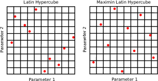
Figure 1.— Examples of a Latin Hypercube (LH) (left) and a Maximin Latin Hypercube (MLH) (right) for a 2D space. The range of each parameter has been divided into $N_{\rm p}=10$ equally spaced intervals, and each point has been located so that any column or row does not contain more than one point. Both designs satisfy the LH condition, but the MLH design generates a better, less clustered, sampling of the space.

3.1.3 Maximum velocity

In order to avoid particles from reaching arbitrarily high velocities, it is convenient to limit the maximum velocity they can acquire. For this reason, we define the maximum velicity as $V_{\rm max}=0.5(X_{\rm max}-X_{\rm min})$ and impose the following restriction

$$v_{k,i}(t)=\begin{cases}v_{k,{\rm max}}&~{}~{}{\rm when}~{}~{}v_{k,i}(t)>v_{k,{\rm max}}\\ -v_{k,{\rm max}}&~{}~{}{\rm when}~{}~{}v_{k,i}(t)<v_{k,{\rm max}}\end{cases}$$ (16)

where $v_{k,i}(t)$ is the $k$-th component of the velocity for the $i$-th particle at timestep $t$ and $v_{k,{\rm max}}$ is the $k$-th component of the maximum velocity defined above. With this condition, the maximum “jump” that a particle can make is equal to half the search space in each dimension.

3.1.4 Boundary conditions

We assume reflecting boundary conditions, where the particle reverses the component of its velocity which is perpendicular to the boundary when it tries to cross it, i.e.

$$v_{k,i}(t)=-v_{k,i}(t)$$ (17)

and

$$x_{k,i}(t)=\begin{cases}x_{k,{\rm max}}&~{}~{}{\rm when}~{}~{}x_{k,i}(t)>x_{k,{\rm max}}\\ x_{k,{\rm min}}&~{}~{}{\rm when}~{}~{}x_{k,i}(t)<x_{k,{\rm min}}\end{cases}$$ (18)

where $x_{k,i}(t)$ and $v_{k,i}(t)$ are the $k$-th component of the position and velocity for the $i$-th particle at timestep $t$, respectively, and $x_{k,{\rm min}}$ and $x_{k,{\rm max}}$ are the $k$-th component of the boundary vectors.

3.1.5 Convergence criterion

In all stochastic methods used to explore multidimensional spaces, the convergence to the region of maximum likelihood is guaranteed only in the asymptotic limit. For that reason, any practical implementation of a stochastic method must include a convergence criterion in order to stop the exploration, thus assuring that the values of the free parameters have reached the convergence region.

PSO particles explore the multidimensional space by finding different values of $G(t)$ as the number of time steps increases. After a certain number of steps, the value of $G(t)$ becomes stationary and the particles cannot find a best global value that is significantly different to the current one. One can take advantage of this and stop the exploration when the following criterion is satisfied:

$$\log_{10}(\bar{\Delta})\leq-2.0,$$ (19)

where

$$\bar{\Delta}=\left<{\bar{x}_{k}(t)-g_{k}(t)\over g_{k}(t)}\right>_{k=1,...,{\rm D}},$$ (20)

and

$$\bar{x}_{k}(t)=\left<x_{k,i}(t)\right>_{i=1,...,N_{\rm p}},$$ (21)

where $x_{k,i}(t)$ is the $k$-th component of the $i$-th particle at step $t$, and $g_{k}(t)$ is the $k$-th component of $G(t)$ at step $t$.

3.2. Estimating errors and degeneracies

The PSO technique is very efficient to find the region of maximum likelihood, but it does not provide a detailed description of the neighbourhood of the best global value, which is needed in order to compute errors and degeneracies. For this reason, to estimate errors we follow the approach presented by Prasad & Souradeep (2012). The procedure involves taking the subset $j=1,...,M$ of sampled points around the final best global position which satisfy

$$|\Theta_{j}|<0.10~{}~{}~{}{\rm with}~{}~{}~{}\Theta_{j}={{X_{j}(t_{\rm f})-G(t_{\rm f})}\over G(t_{\rm f})},$$ (22)

where $t_{\rm f}$ is the final step. In this neighbourhood of the best-fitting point, the fitness function can be approximated by

$$F_{j}(t_{\rm f})\simeq F^{\rm max}(\rm t_{\rm f})\exp{\left(-{1\over 2}\Theta_{\it j}^{\rm T}\mathbf{R}\Theta_{\it j}\right)},$$ (23)

where $\mathbf{R}$ is the D$\times$D curvature matrix. The inverse of this matrix is the covariance matrix $\mathbf{C}$, which can be used to estimate the error and degeneracies of the parameters around the best global value (Jungman et al., 1996). Taking

$$\Delta_{j}^{2}=-2~{}{\rm ln}\left[{F_{j}(t_{\rm f})\over F^{\rm max}(t_{\rm f})}\right]=\Theta_{j}^{\rm T}\mathbf{R}\Theta_{j},$$ (24)

a D-dimensional paraboloid can be fitted to the $\left\{\Delta^{2}_{j}\right\}_{j=1,...,M}$ subset to obtain the D(D+1)/2 independent coefficients of the matrix $\mathbf{R}$. The covariance matrix is then computed taking the inverse of the curvature matrix, i.e. $\mathbf{C}=\mathbf{R}^{-1}$. The error $\sigma_{k}$ of the $k$-th parameter is computed using the diagonal elements of $\mathbf{C}$,

$$\sigma_{k}=g_{k}(t)\sqrt{C_{kk}},$$ (25)

and the off-diagonal elements are used to approximate the possible degeneracies between parameters.

4. Constraints for the calibrations

4.1. Observational data

To calibrate SAG using the PSO method, we compare the properties of the simulated galaxies with two observationally-determined statistics focused on the stellar mass content and central SMBH masses of galaxies, both at $z=0$. These constraints are the stellar mass function (SMF) and the BH mass to bulge mass relation (BHB):

(1) The stellar mass function at $z=0$ (SMF). We calibrate with the data used by Henriques et al. (2014), which is a combination of the SMF of the Sloan Digital Sky Survey (SDSS) from Baldry et al. (2008) and Li & White (2009), and of the Galaxy And Mass Assembly (GAMA) from Baldry et al. (2012).

(2) The BH mass to bulge mass relation (BHB). We combine the datasets from McConnell & Ma (2013) and Kormendy & Ho (2013). The data points used are the average of the BH mass computed over several bulge mass bins, with errors estimated as the dispersion around that average.

The use of SMF to constrain parameters of SAMs is standard practice (Mutch et al., 2013a, b; Henriques et al., 2013, 2014; Benson, 2014). The local SMF is an ideal constraint to evaluate the impact of the physical processes included in galaxy formation models. In particular, the low mass end reflects the effect of SNe feedback, whereas the break and high mass end are directly associated with the impact of AGN feedback (e.g. Benson et al. 2003; Bower et al. 2006; Lagos et al. 2008). Additionally, if a prescription for AGN feedback is implemented (as is the case in SAG), the BHB relationship is a necessary constraint that must also be satisfied.

4.2. Likelihood function

As mentioned in Sec. 3, for a given position $X$ (i.e., a particular parameter set) and a given observational property, the likelihood of the model is computed according to

$$F(X)\propto\exp{\left(-0.5\chi^{2}\right)},$$ (26)

with

$$\chi^{2}=\sum_{i=1}^{N_{\rm bin}}{{\left(y_{{\rm sag},i}-y_{{\rm obs},i}\right)^{2}}\over{\sigma^{2}_{{\rm sag},i}+\sigma^{2}_{{\rm obs},i}}}$$ (27)

where $N_{\rm bin}$ is the number of data bins and $y_{{\rm sag},i}$ and $y_{{\rm obs},i}$ are the $i$-th values of a given constraint for the SAG model and observations, respectively. The values of $\sigma_{{\rm sag},i}$ and $\sigma_{{\rm obs},i}$ are the errors for the $i$-th bin for SAG and the observations, where $\sigma_{{\rm sag},i}$ is computed as a Poisson error.

The final likelihood assigned to a position $X$ is given by the product of the likelihoods of all $N_{\rm c}$ constraints used in a particular calibration,

$$F(X)\propto\exp{\left(-0.5\sum_{i=1}^{N_{\rm c}}{\chi^{2}_{i}}\right)}$$ (28)

It is important to note that when we take the direct sum of the $\chi^{2}$ to the different constraints to compute the final likelihood, for the sake of simplicity we are not taking into account the correlation between bins and observables, which may be non-negligible (Benson, 2014).

5. Results

5.1. Best fit values

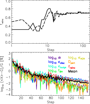
Figure 2.— In the top panel we show an example of the temporal evolution of the best global value $G(t)$ (solid lines) and the average $\left<X_{i}(t)\right>_{i=1,...,N_{\rm p}}$ (dashed lines) for the $f_{\rm reinc}$ parameter. The $y$-axis corresponds to the range explored. Bottom panel shows the relative difference between the average particle parameters and the best global value, which is used as convergence criterion.

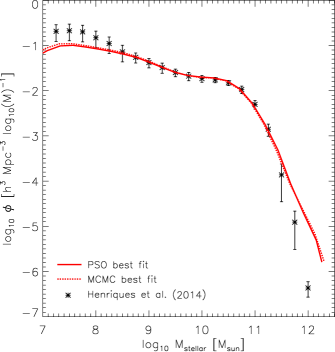
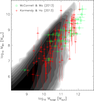
Figure 3.— Comparison between the results of the calibrated model and the observational constraints used. Left panel: SMF at $z=0$ obtained from the SAG model calibrated with PSO (red solid line) and with MCMC (red dotted line); black symbols depict the data compilation of Henriques et al. (2014). Right panel: BHB relation obtained from SAG galaxies calibrated with PSO (grey contours); results of the calibration with MCMC are not showed for clarity. The contours represent the normalized density of the total population of model galaxies that contain a black hole. Symbols represent the data from McConnell & Ma (2013) (green squares) and Kormendy & Ho (2013) (red rhombus).

We consider the observational constraints described in Sec. 4 to calibrate the SAG model. We use $N_{\rm p}=30$ particles to search for the best fit according to the observational constraints in the chosen seven-dimensional parameter space. As mentioned in Sec. 3, the number of particles $N_{\rm p}$ is a free parameter of the PSO algorithm and there is no particular criterion to choose a value. In PSOS06, the suggestion for the number of particles of the swarm is given by $N_{\rm p}=10+2\sqrt{D}$, where $D$ is the dimension of the space. According to this, we obtain $N_{\rm p}\sim 15$ for our study. We choose to increase the value to $30$ to have a better sampling of the parameter space and ensure that similar results –in terms of the best-fitting value– are obtained when identical calibrations are performed.

The top panel of Fig. 2 shows an example of the evolution of the best global value $G(t)$ (solid line) and the corresponding average value $\left<X_{i}(t)\right>_{i=1,N_{\rm p}}$ (dashed line) of all PSO particles as a function of the step $t$ for one of the free parameters, $f_{\rm reinc}$. A small difference between the global and the average values indicates convergence to the best set of parameters. We define the accuracy of convergence for each parameter in terms of the relative difference between the average parameter of all the particles and the final best-fitting global value $G(t)$. The relative difference among all parameters (black line in bottom panel of Fig. 2) is used as the convergence criterion; the PSO exploration stops when this difference is smaller than 10^-2 per cent. We can see that the parameters converge in $\sim 150$ steps, which corresponds to $\sim 4500$ evaluations of the SAG model.

Table 1Best-fitting parameters found with the PSO and MCMC techniques

. Parameter $X_{\rm min}$ $X_{\rm max}$ PSO MCMC $\alpha$ $0.001$ $1.0$ $0.023\pm 0.004$ $0.022^{+0.003}_{-0.006}$ $\epsilon_{\rm disc}$ $0.001$ $1.0$ $0.19\pm 0.01$ $0.21^{+0.07}_{-0.05}$ $\epsilon_{\rm bulge}$ $0.001$ $1.0$ $0.19\pm 0.03$ $0.22^{+0.07}_{-0.09}$ $f_{\rm BH}$ $0.01$ $1.0$ $0.078\pm 0.005$ $0.08^{+0.03}_{-0.03}$ $10^{3}\kappa_{\rm AGN}$ $0.001$ $10.0$ $0.08\pm 0.01$ $0.08^{+0.08}_{-0.04}$ $D_{\rm pert}$ $0.0$ $60.0$ $47\pm 3$ $49^{+5}_{-6}$ $f_{\rm reinc}$ $0.0$ $1.0$ $0.70\pm 0.02$ $0.66^{+0.15}_{-0.22}$

The global best-fitting values found for the calibration done with the PSO technique are listed in Table 1 together with the search ranges $[X_{\rm min},X_{\rm max}]$ and the error estimates obtained according to the method described in Sec. 3.2. The reduced chi-square obtained for the SMF is $\chi^{2}=0.523$ and for the BHB is $\chi^{2}=0.208$.

Fig. 3 shows the results given by the calibrated model for the statistics involved in the calibration process compared with the corresponding observational data. As expected, both observational constraints (SMF at $z=0$ and BHB relation) are well reproduced. The discrepancies with observational data at the low and high mass end of the $z=0$ SMF denote some drawbacks in the model related with the SNe feedback and/or the ejection-reincorporation scheme, whose effects impact the low mass end, and the AGN feedback that has strong influence on the high mass end. The latter aspect is also reflected in the BHB relation obtained from the model, which appears to depart from the observed data for galaxies with high bulge masses. Since the SMF constraint is stronger than the one imposed by the BHB relation, the model generates BH with somewhat larger masses than observed for a galaxy with a given bulge mass in order to produce a larger AGN feedback that can bring the high mass end of the SMF in better agreement with observations. However, taking into consideration the high amount of scatter present in the observational data of the BHB relation, the calibration can be said to reproduce it satisfactorily.

These results show the good performance of the PSO method when applied to the calibration process of a SAM. In order to evaluate the advantages of this technique with respect to MCMC, we implement the latter method to calibrate our model using the same set of free parameters and observational constraints. For this work we run a MCMC of $\sim 30000$ steps using the Metropolis-Hastings algorithm (Metropolis et al., 1953; Hastings, 1970), where the tipical length for SAMs calibrations is between $10^{4}$ and $10^{5}$ steps in order to achieve some level of convergence to the maximum likelihood region (Henriques et al., 2009, 2013; Mutch et al., 2013b). This MCMC allows us to explore the parameter space with more detail (see Sec. 5.2). The resulting best fit value found by the MCMC is also presented in Table 1, with the corresponding $2\sigma$ confidence levels. In this case, the reduced chi-square obtained for the SMF is $\chi^{2}=0.513$ and for the BHB is $\chi^{2}=0.212$. As can be seen, the parameter values and the final likelihood do not differ significantly from those found with the PSO algorithm, being statistically consistent. This fact is reflected in the left panel of Fig. 3, where the SMF at $z=0$ resulting from the MCMC calibration is also shown. As can be seen, the SMF predicted by PSO and MCMC are indistinguishable. The principal difference between these two results are the errorbars, being those obtained with MCMC significantly larger. At this point we need to emphasize that for the PSO method we estimate errors according to the fitting procedure described in Sec. 3.2, therefore, the errors in the PSO method must be interpreted just as an approximation of the true uncertainties.

With this comparison, we demonstrate that the PSO method gives a definite advantage with respect to MCMC showing convergence to the same region of maximum likelihood in a considerably smaller computing time. This is reaffirmed through the analysis of the parameter space in the next section.

5.2. The parameter space

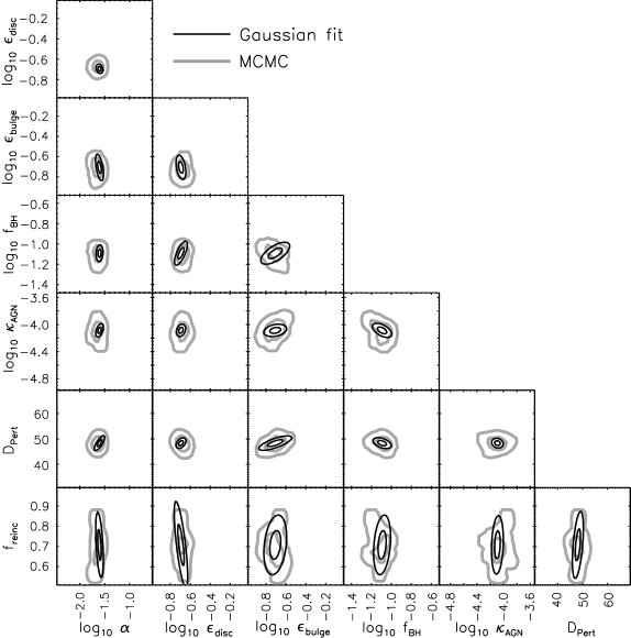
Figure 4.— 2D projections of the multidimensional Gaussian fit described in Sec. 3.2 (black thin lines; concentric contours represent the $0.01$ and $0.5$ levels of the normalised Gaussian), and the $68$ and $95$ per cent preferred regions of the MCMC (thick grey lines). The projections allow us to infer information about the degeneracies present between the free parameters of the model.

As mentioned in Sec. 3.2, the PSO algorithm is extremely efficient at finding the region of maximum likelihood of a multidimensional parameter space, but at the expense of not providing a detailed description of the neighbourhood of this region. However, the fitting procedure presented in Sec. 3.2 allows us to obtain an estimation of the parameter degeneracies.

In Fig. 4 we show the 2D projections of the multidimensional Gaussian fit (black thin curves) applied in the neighbourhood of the best-fitting parameters found with PSO. The two concentric contours represent the $0.01$ and $0.5$ levels of the normalised Gaussian (see Eq. 23). In addition, grey thick curves show the $68$ and $95$ per cent preferred regions of the MCMC exploration performed. It is clear from this figure that the fitting procedure gives us a decent approximation of the degeneracies in the parameter space: all the degeneracies present in the projected Gaussians (with the exception of the $f_{\rm BH}-\epsilon_{\rm bulge}$ degeneracy) agree with the true ones found with the MCMC sampling. It is important to recall that the contours of the projected Gaussians do not represent the same information that the contours of the MCMC (the second is a true sampling of the parameter space while the first responds to a fitted curvature matrix in a limited subsample of points of the region of maximum likelihood), therefore, as we mentioned in Sec. 5.1, this projected fit must be interpreted just as a merit figure of the true topology of the parameter space.

The previous considerations demonstrate that the PSO method, combined with the fitting procedure of Sec. 3.2, also allows us to infer information about the parameter degeneracies with no extra evaluations of the model. However, it is important to emphasize that if an exhaustive exploration of the parameter space is needed, the PSO method must be used only to locate the region of the maximum likelihood, and the complementary exploration should be done using other additional exploration tools, as for instance a localised MCMC.

6. Conclusions

Semi-analytic models of galaxy formation are characterised by a set of free parameters that regulate the effect of the physical processes involved in shaping the properties of the galaxy population. We have shown that the PSO technique can be successfully employed to find the best-fitting set of parameters for a SAM. For the particular calibration performed in this work, the PSO method find the same region of maximum likelihood with 1 order of magnitude less evaluations than using the traditional MCMC methods, as it has been already reported by Prasad & Souradeep (2012). In this work, we apply the PSO technique to the SAG galaxy formation model (Cora, 2006; Lagos et al., 2008; Padilla et al., 2014; Gargiulo et al., 2014), but this method could be applied to any other SAM.

We test the PSO algorithm on SAG by performing a calibration of seven free parameters of the model using two observational constraints at $z=0$: the stellar mass function and the black hole to bulge mass relation. Once the PSO converges to the best parameter set (i.e., the region of maximum likelihood), we estimate errors and degeneracies between parameters using the fitting procedure described in Sec. 3.2. To validate these results, we also perform a MCMC exploration, finding the same results not only in terms of parameter and likelihood values (Fig. 3 and Sec. 5.1), but also in terms of the insights of the topology of the parameter space (Fig. 4 and Sec. 5.2). The principal advantage of the PSO algorithm over the traditional MCMC explorations is the computational cost: while the PSO algorithm needs $\sim 4500$ valuations, the MCMC requires $\sim 1$ order of magnitude more. However, it is fair to remark that the PSO algorithm is a suitable tool to locate “maximum values”, whereas the MCMC provides a full exploration method of the parameter space.

It should be noted that in this work we have only explored parameters related to the baryonic physics, assuming a fixed cosmological background. However, this SAM calibration will very likely change if the cosmological parameters (i.e. $\Omega_{\rm m}$, $\Omega_{\rm b}$, $\sigma_{8}$, etc.) are modified. Recently, useful techniques to scale the cosmology of (sub)halo catalogues extracted from N-body simulations were introduced, such as Angulo & White (2010), Ruiz et al. (2011) and Mead & Peacock (2014). Using these techniques, the parameter space of SAMs can be further extended in order to include both baryonic and cosmological parameters. As the parameter space of galaxy formation models grows, it becomes even more complicated to calibrate such models by hand; therefore, calibration methods such as the one introduced in this paper become a necessity. In further works we will explore such extended parameter spaces with the new capabilities provided by the efficient PSO method.

References

- Angulo et al. (2012) Angulo, R. E., Springel, V., White, S. D. M., Jenkins, A., Baugh, C. M., & Frenk, C. S. 2012, MNRAS, 426, 2046
- Angulo & White (2010) Angulo, R. E. & White, S. D. M. 2010, MNRAS, 405, 143
- Baldry et al. (2012) Baldry, I. K., Driver, S. P., Loveday, J., Taylor, E. N., Kelvin, L. S., Liske, J., Norberg, P., Robotham, A. S. G., Brough, S., Hopkins, A. M., Bamford, S. P., Peacock, J. A., Bland-Hawthorn, J., Conselice, C. J., Croom, S. M., Jones, D. H., Parkinson, H. R., Popescu, C. C., Prescott, M., Sharp, R. G., & Tuffs, R. J. 2012, MNRAS, 421, 621
- Baldry et al. (2008) Baldry, I. K., Glazebrook, K., & Driver, S. P. 2008, MNRAS, 388, 945
- Baugh (2006) Baugh, C. M. 2006, Rep. Prog. Phys., 69, 3101
- Benson (2010) Benson, A. J. 2010, Physics Reports, 495, 33
- Benson (2014) —. 2014, MNRAS, 444, 2599
- Benson et al. (2012) Benson, A. J., Borgani, S., De Lucia, G., Boylan-Kolchin, M., & Monaco, P. 2012, MNRAS, 419, 3590
- Benson et al. (2003) Benson, A. J., Bower, R. G., Frenk, C. S., Lacey, C. G., Baugh, C. M., & Cole, S. 2003, ApJ, 599, 38
- Bertschinger (2001) Bertschinger, E. 2001, ApJS, 137, 1
- Bondi (1952) Bondi, H. 1952, MNRAS, 112, 195
- Bower et al. (2010) Bower, R., Vernon, I., Goldstein, M., Benson, A., Lacey, C., Baugh, C., Cole, S., & Frenk, C. 2010, MNRAS, 407, 2017
- Bower et al. (2006) Bower, R. G., Benson, A. J., Malbon, R., Helly, J. C., Frenk, C. S., Baugh, C. M., Cole, S., & Lacey, C. G. 2006, MNRAS, 370, 645
- Boylan-Kolchin et al. (2009) Boylan-Kolchin, M., Springel, V., White, S. D. M., Jenkins, A., & Lemson, G. 2009, MNRAS, 398, 1150
- Chabrier (2003) Chabrier, G. 2003, PASP, 115, 763
- Cora (2006) Cora, S. A. 2006, MNRAS, 368, 1540
- Croton et al. (2006) Croton, D. J., Springel, V., White, S. D. M., De Lucia, G., Frenk, C. S., Gao, L., Jenkins, A., Kauffmann, G., Navarro, J. F., & Yoshida, N. 2006, MNRAS, 365, 11
- De Lucia et al. (2004) De Lucia, G., Kauffmann, G., & White, S. D. M. 2004, MNRAS, 349, 1101
- Efstathiou et al. (1982) Efstathiou, G., Lake, G., & Negroponte, J. 1982, MNRAS, 199, 1069
- Foster et al. (2012) Foster, A. R., Ji, L., Smith, R. K., & Brickhouse, N. S. 2012, ApJ, 756, 128
- Frenk & White (2012) Frenk, C. S. & White, S. D. M. 2012, Annalen der Physik, 524, 507
- Gargiulo et al. (2014) Gargiulo, I. D., Cora, S. A., Padilla, N. D., Muñoz Arancibia, A. M., Ruiz, A. N., Orsi, A., Tecce, T. E., Weidner, C., & Bruzual, G. 2014, MNRAS, in press (arXiv:astro-ph/1402.3296)
- Gómez et al. (2012) Gómez, F. A., Coleman-Smith, C. E., O’Shea, B. W., Tumlinson, J., & Wolpert, R. L. 2012, ApJ, 760, 112
- Gómez et al. (2014) —. 2014, ApJ, 787, 20
- Greggio & Renzini (1983) Greggio, L. & Renzini, A. 1983, AA, 118, 217
- Guo et al. (2011) Guo, Q., White, S., Boylan-Kolchin, M., De Lucia, G., Kauffmann, G., Lemson, G., Li, C., Springel, V., & Weinmann, S. 2011, MNRAS, 413, 101
- Hastings (1970) Hastings, W. K. 1970, Biometrika, 57, 97
- Henriques et al. (2014) Henriques, B., White, S., Thomas, P., Angulo, R., Guo, Q., Lemson, G., Springel, V., & Overzier, R. 2014, arXiv/astro-ph:1410.0365
- Henriques & Thomas (2010) Henriques, B. M. B. & Thomas, P. A. 2010, MNRAS, 403, 768
- Henriques et al. (2009) Henriques, B. M. B., Thomas, P. A., Oliver, S., & Roseboom, I. 2009, MNRAS, 396, 535
- Henriques et al. (2013) Henriques, B. M. B., White, S. D. M., Thomas, P. A., Angulo, R. E., Guo, Q., Lemson, G., & Springel, V. 2013, MNRAS, 431, 3373
- Hirschi et al. (2005) Hirschi, R., Meynet, G., & Maeder, A. 2005, AA, 433, 1013
- Iwamoto et al. (1999) Iwamoto, K., Brachwitz, F., Namoto, K., Kishimoto, N., Umeda, H., Hix, W. R., & Thielemann, F. 1999, ApJS, 125, 439
- Jarosik et al. (2011) Jarosik, N., Bennett, C. L., Dunkley, J., Gold, B., Greason, M. R., Halpern, M., Hill, R. S., Hinshaw, G., Kogut, A., Komatsu, E., Larson, D., Limon, M., Meyer, S. S., Nolta, M. R., Odegard, N., Page, L., Smith, K. M., Spergel, D. N., Tucker, G. S., Weiland, J. L., Wollack, E., & Wright, E. L. 2011, ApJS, 192, 14
- Jungman et al. (1996) Jungman, G., Kamionkowski, M., Kosowsky, A., & Spergel, D. N. 1996, Phys. Rev. D, 54, 1332
- Kampakoglou et al. (2008) Kampakoglou, M., Trotta, R., & Silk, J. 2008, MNRAS, 384, 1414
- Karakas (2010) Karakas, A. I. 2010, MNRAS, 403, 1413
- Kennedy & Eberhart (1995) Kennedy, J. & Eberhart, R. C. 1995, IEEE, 4, 1992
- Kennedy & O’Hagan (2001) Kennedy, M. C. & O’Hagan, A. 2001, Journal of the Royal Statistical Society, Series B, 63, 425
- Klypin et al. (2011) Klypin, A. A., Trujillo-Gomez, S., & Primack, J. 2011, ApJ, 740, 102
- Kobayashi et al. (2006) Kobayashi, C., Umeda, H., Nomoto, K., Tominaga, N., & Ohkubo, T. 2006, ApJ, 653, 1145
- Kormendy & Ho (2013) Kormendy, J. & Ho, L. C. 2013, ARAA, 51, 511
- Lagos et al. (2008) Lagos, C., Cora, S., & Padilla, N. D. 2008, MNRAS, 388, 587
- Li & White (2009) Li, C. & White, S. D. M. 2009, MNRAS, 398, 2177
- Lia et al. (2002) Lia, C., Portinari, L., & Carraro, G. 2002, MNRAS, 330, 821
- Lu et al. (2012) Lu, Y., Mo, H. J., Katz, N., & Weinberg, M. D. 2012, MNRAS, 421, 1779
- Lu et al. (2011) Lu, Y., Mo, H. J., Weinberg, M. D., & Katz, N. 2011, MNRAS, 416, 1949
- McConnell & Ma (2013) McConnell, N. J. & Ma, C.-P. 2013, ApJ, 764, 184
- McKay et al. (1979) McKay, M. D., Beckman, R. J., & Conover, W. J. 1979, Technometrics, 21, 239
- Mead & Peacock (2014) Mead, A. J. & Peacock, J. A. 2014, MNRAS, 440, 1233
- Melinder et al. (2012) Melinder, J., Dahlen, T., Mencía Trinchant, L., Östlin, G., Mattila, S., Sollerman, J., Fransson, C., Hayes, M., Kankare, E., & Nasoudi-Shoar, S. 2012, A&A, 545, A96
- Metropolis et al. (1953) Metropolis, N., Rosenbluth, A., Rosenbluth, M. M., Teller, A., & Teller, E. 1953, JCP, 21, 1087
- Mo et al. (1998) Mo, H. J., Mao, S., & White, S. D. M. 1998, MNRAS, 295, 319
- Mutch et al. (2013a) Mutch, S. J., Croton, D. J., & Poole, G. B. 2013a, MNRAS, 435, 2445
- Mutch et al. (2013b) Mutch, S. J., Poole, G. B., & Croton, D. J. 2013b, MNRAS, 428, 2001
- Padilla et al. (2014) Padilla, N. D., Salazar-Albornoz, S., Contreras, S., Cora, S. A., & Ruiz, A. N. 2014, MNRAS, 443, 2801
- Padovani & Matteucci (1993) Padovani, P. & Matteucci, F. 1993, ApJ, 416, 26
- Prasad & Souradeep (2012) Prasad, J. & Souradeep, T. 2012, Phys. Rev. D, 85, 123008
- Rogers & Fiege (2011) Rogers, A. & Fiege, J. D. 2011, ApJ, 727, 80
- Romano et al. (2010) Romano, D., Karakas, A. I., Tosi, M., & Matteucci, F. 2010, AA, 522, A32
- Ruiz et al. (2011) Ruiz, A. N., Padilla, N. D., Domínguez, M. J., & Cora, S. A. 2011, MNRAS, 418, 2422
- Silk & Mamon (2012) Silk, J. & Mamon, G. A. 2012, Research in Astronomy and Astrophysics, 12, 917
- Skokos et al. (2005) Skokos, C., Parsopoulos, K. E., Patsis, P. A., & Vrahatis, M. N. 2005, MNRAS, 359, 251
- Springel (2005) Springel, V. 2005, MNRAS, 364, 1105
- Springel et al. (2005) Springel, V., White, S. D. M., Jenkins, A., Frenk, C. S., Yoshida, N., Gao, L., Navarro, J., Thacker, R., Croton, D., Helly, J., Peacock, J. A., Cole, S., Thomas, P., Couchman, H., Evrard, A., Colberg, J., & Pearce, F. 2005, Nature, 435, 629
- Springel et al. (2001) Springel, V., White, S. D. M., Tormen, G., & Kauffmann, G. 2001, MNRAS, 328, 726
- Stein (1987) Stein, M. 1987, Technometrics, 29, 143151
- Wang & Mohanty (2010) Wang, Y. & Mohanty, S. D. 2010, Phys. Rev. D, 81, 063002