What Next-Generation 21 cm Power Spectrum Measurements Can Teach Us About the Epoch of Reionization

Abstract

A number of experiments are currently working towards a measurement of the 21 cm signal from the Epoch of Reionization. Whether or not these experiments deliver a detection of cosmological emission, their limited sensitivity will prevent them from providing detailed information about the astrophysics of reionization. In this work, we consider what types of measurements will be enabled by a next-generation of larger 21 cm EoR telescopes. To calculate the type of constraints that will be possible with such arrays, we use simple models for the instrument, foreground emission, and the reionization history. We focus primarily on an instrument modeled after the $\sim 0.1~{}\rm{km}^{2}$ collecting area Hydrogen Epoch of Reionization Array (HERA) concept design, and parameterize the uncertainties with regard to foreground emission by considering different limits to the recently described “wedge” footprint in $k$-space. Uncertainties in the reionization history are accounted for using a series of simulations which vary the ionizing efficiency and minimum virial temperature of the galaxies responsible for reionization, as well as the mean free path of ionizing photons through the IGM. Given various combinations of models, we consider the significance of the possible power spectrum detections, the ability to trace the power spectrum evolution versus redshift, the detectability of salient power spectrum features, and the achievable level of quantitative constraints on astrophysical parameters. Ultimately, we find that $0.1~{}\rm{km}^{2}$ of collecting area is enough to ensure a very high significance ($\gtrsim 30\sigma$) detection of the reionization power spectrum in even the most pessimistic scenarios. This sensitivity should allow for meaningful constraints on the reionization history and astrophysical parameters, especially if foreground subtraction techniques can be improved and successfully implemented.

1. Introduction

The Epoch of Reionization (EoR) represents a turning point in cosmic history, signaling the moment when large scale structure has become significant enough to impart a global change to the state of the baryonic universe. In particular, the EoR is the period when ultraviolet photons (likely from the first galaxies) reionize the neutral hydrogen in the intergalactic medium (IGM). As such, measurements of the conditions during the EoR promise a wealth of information about the evolution of structure in the universe. Observationally, the redshift of EoR is roughly constrained to be between $z\sim 6\mbox{--}13$, with a likely extended duration; see Furlanetto et al. (2006b), Barkana & Loeb (2007), and Loeb & Furlanetto (2013) for reviews of the field. Given the difficulties of optical/NIR observing at these redshifts, the highly-redshifted 21 cm line of neutral hydrogen has been recognized as a unique probe of the conditions during the EoR (see Morales & Wyithe 2010 and Pritchard & Loeb 2012 for recent reviews discussing this technique).

In the last few years, the first generation of experiments targeting a detection of this highly-redshifted 21 cm signal from the EoR has come to fruition. In particular, the LOw Frequency ARray (LOFAR; Yatawatta et al. 2013; van Haarlem et al. 2013), the Murchison Widefield Array (MWA; Tingay et al. 2013; Bowman et al. 2013), and the Donald C. Backer Precision Array for Probing the Epoch of Reionization (PAPER; Parsons et al. 2010) have all begun long, dedicated campaigns with the goal of detecting the 21 cm power spectrum. Ultimately, the success or failure of these campaigns will depend on the feasibility of controlling both instrumental systematics and foreground emission. But even if these challenges can be overcome, a positive detection of the power spectrum will likely be marginal at best because of limited collecting area. Progressing from a detection to a characterization of the power spectrum (and eventually, to the imaging of the EoR) will require a next generation of larger 21 cm experiments.

The goal of this paper is to explore the range of constraints that could be achievable with larger 21 cm experiments and, in particular, focus on how those constraints translate into a physical understanding of the EoR. Many groups have analyzed the observable effects of different reionization models on the 21 cm power spectrum; see e.g., Zaldarriaga et al. (2004), Furlanetto et al. (2004), McQuinn et al. (2006), Bowman et al. (2006), Bowman et al. (2007), Trac & Cen (2007), Lidz et al. (2008), and Iliev et al. (2012). These studies did not include the more sophisticated understanding of foreground emission that has arisen in the last few years, i.e., the division of 2D cylindrical $k$-space into the foreground-contaminated “wedge” and the relatively clean “EoR window” (Datta et al., 2010; Vedantham et al., 2012; Morales et al., 2012; Parsons et al., 2012b; Trott et al., 2012; Thyagarajan et al., 2013). The principal undertaking of this present work is to reconcile these two literatures, exploring the effects of both different EoR histories and foreground removal models on the recovery of astrophysical information from the 21 cm power spectrum. Furthermore, in this work we present some of the first analysis focused on using realistic measurements to distinguish between different theoretical scenarios, rather than simply computing observable (but possibly degenerate) quantities from a given theory. The end result is a set of generic conclusions that both demonstrates the need for a large collecting area next generation experiment and motivates the continued development of foreground removal algorithms.

In order to accomplish these goals, this paper will employ simple models designed to encompass a wide range of possible scenarios. These models are described in §2, wherein we describe the models for the instrument (§2.1), foregrounds (§2.2), and reionization history (§2.3). In §3, we present a synthesis of these models and the resultant range of potential power spectrum constraints, including a detailed examination of how well one can recover physical parameters describing the EoR in §3.5. In §4, we conclude with several generic messages about the kind of science the community can expect from 21 cm experiments in the next $\sim 5$ years.

2. The Models

In this section we present the various models for the instrument (§2.1), foreground removal (§2.2), and reionization history (§2.3) used to explore the range of potential EoR measurements. In general, these models are chosen not because they necessarily mirror specific measurements or scenarios, but rather because of their simplicity while still encompassing a wide range of uncertainty about many parameters. We choose several different parameterizations of the foreground removal algorithms, and use simple simulations to probe a wide variety of reionization histories. Our model telescope (described below in §2.1) is based off the proposed Hydrogen Epoch of Reionization Array (HERA); we present sensitivity calculations and astrophysical constraints for other 21 cm experiments in the appendix.

2.1. The Telescope Model

The most significant difference between the current and next generations of 21 cm instruments will be a substantial increase in collecting area and, therefore, sensitivity. In the main body of this work, we use an instrument modeled after a concept design for the Hydrogen Epoch of Reionization Array (HERA). This array consists of 547 zenith-pointing 14 m diameter reflecting-parabolic elements in a close-packed hexagon, as shown in Figure 1.

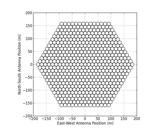
Figure 1.— The 547-element, hexagonally packed HERA concept design, with 14 m reflector elements. Outrigger antennas may be included in the final design for the purposes of foreground imaging, but they are not treated here, since they add little to power spectrum sensitivity.

The total collecting area of this array is $84,000~{}\rm{m}^{2}$, or approximately one tenth of a square kilometer. The goal of this work is not to justify this particular design choice, but rather to show that this scale instrument enables a next level of EoR science beyond the first generation experiments. In the appendix, we present the resultant sensitivities and achievable constraints on the astrophysical parameters of interest for several other 21 cm telescopes: PAPER, the MWA, LOFAR, and a concept design for the SKA-Low Phase 1. Generically, we find that power spectrum sensitivities are a strong function of array configuration, especially compactness and redundancy. However, once the power spectrum sensitivity of an array is known, constraints on reionization physics appear to be roughly independent of other paramters.

In many ways, the HERA concept array design is quite representative of 21 cm EoR experiments over the next $\sim 5\mbox{--}10$ years. As mentioned, it has a collecting area of order a tenth of a square kilometer — significantly larger than any current instrument, but smaller than Phase 1 of the low-frequency Square Kilometre Array (SKA1-low). (See Table LABEL:tab:instruments for a summary of different EoR telescopes.) In terms of power spectrum sensitivity, Parsons et al. (2012a) demonstrated the power of array redundancy for reducing thermal noise uncertainty, and showed that a hexagonal configuration has the greatest instantaneous redundancy. In this sense, the HERA concept design is optimized for power spectrum measurements. Other configurations in the literature have been optimized for foreground imaging or other additional science; the purpose of this work is not to argue for or against these designs. Rather, we concentrate primarily on science with the 21 cm power spectrum, and use the HERA concept design as representative of power spectrum-focused experiments. Obviously, arrays with more (less) collecting area will have correspondingly greater (poorer) sensitivity. The key parameters of our fiducial concept array are given in Table LABEL:tab:array, and constraints achievable with other arrays are presented in the appendix.

[caption=Fiducial System Parameters, label=tab:array, pos=ht, mincapwidth=3.5in]c—c Observing Frequency $50\mbox{--}225$ MHz
$T_{\rm receiver}$ 100 K
Parabolic Element Size 14 m
Number of Elements 547
Primary beam size $8.7^{\circ}$ FWHM at 150 MHz
Configuration Close-packed hexagonal
Observing mode Drift-scanning at zenith

2.1.1 Calculating Power Spectrum Sensitivity

To calculate the power spectrum sensitivity of our fiducial array, we use the method presented in Pober et al. (2013b), which is briefly summarized here. This method begins by creating the $uv$ coverage of the observation by gridding each baseline into the $uv$ plane, including the effects of earth-rotation synthesis over the course of the observation. We choose $uv$ pixels the size of the antenna element in wavelengths, and assume that any baseline samples only one pixel at a time. Each pixel is treated as an independent sample of one $k_{\perp}$-mode, along which the instrument samples a wide range of $k_{\parallel}$-modes specified by the observing bandwidth. The sensitivity to any one mode of the dimensionless power spectrum is given by Equation (4) in Pober et al. (2013b), which is in turn derived from Equation (16) of Parsons et al. (2012a):

$$\Delta^{2}_{\rm N}(k)\approx X^{2}Y\frac{k^{3}}{2\pi^{2}}\frac{\Omega^{\prime}}{2t}T_{\rm sys}^{2},$$ (1)

where $X^{2}Y$ is a cosmological scalar converting observed bandwidths and solid angles to $h{\rm Mpc}^{-1}$, $\Omega^{\prime}\equiv\Omega_{\rm p}^{2}/\Omega_{\rm pp}$ is the solid angle of the power primary beam ($\Omega_{\rm p}$) squared, divided by the solid angle of the square of the power primary beam ($\Omega_{\rm pp}$), $t$ is the integration time on that particular $k$-mode, and $T_{\rm sys}$ is the system temperature. It should also be noted that this equation is dual-polarization, i.e., it assumes both linear polarizations are measured simultaneously and then combined to make a power spectrum estimate. Similar forms of this equation appear in Morales (2005) and McQuinn et al. (2006) which differ only by the polarization factor and power-squared primary beam correction.

In our formalism, each measured mode is attributed a noise value calculated from Equation 1 (see §2.1.2 for specifics on the values of each parameter). Independent modes can be combined in quadrature to form spherical or cylindrical power spectra as desired. One has a choice of how to combine non-instantaneously redundant baselines which do in fact sample the same $k_{\perp}/uv$ pixel. Such a situation can arise either through the effect of the gridding kernel creating overlapping $uv$ footprints on similar length baselines (“partial coherence”; Hazelton et al. 2013), or through the effect of earth-rotation bringing a baseline into a $uv$ pixel previously sampled by another baseline. Naïvely, this formalism treats these samples as perfectly coherent, i.e., we add the integration time of each baseline within a $uv$ pixel. As suggested by Hazelton et al. (2013), however, it is possible that this kind of simple treatment could lead to foreground contamination in a large number of Fourier modes. To explore the ramifications of this effect, we will also consider a case where only baselines which are instantaneously redundant are added coherently, and all other measurements are added in quadrature when binning. We discuss this model more in §2.2.

Since this method of calculating power spectrum sensitivities naturally tracks the number of independent modes measured, sample variance is easily included when combining modes by adding the value of the cosmological power spectrum to each $(u,v,\eta)$-voxel (where $\eta$ is the line-of-sight Fourier mode) before doing any binning. (Note that in the case where only instantaneously redundant baselines are added coherently, partially coherent baselines do not count as independent samples for the purpose of calculating sample variance.) Unlike Pober et al. (2013b), we do not include the effects of redshift-space distortions in boosting the line of sight signal, since they will not boost the power spectrum of ionization fluctuations, which is likely to dominate the 21 cm power spectrum at these redshifts. We also ignore other second order effects on the power spectrum, such as the “light-cone” effect (Datta et al., 2012; La Plante et al., 2013).

2.1.2 Telescope and Observational Parameters

For the instrument value of $T_{\rm sys}$ we sum a frequency independent 100 K receiver temperature with a frequency dependent sky temperature, $T_{\rm sky}=60\rm{K}~{}(\lambda/1~{}{\rm m})^{2.55}$ (Thompson et al., 2007), giving a sky temperature of 351 K at 150 MHz. Although this model is $\sim 100$ K lower than the system measured by Parsons et al. (2013), it is consistent with recent LOFAR measurements (Yatawatta et al., 2013; van Haarlem et al., 2013). Since the smaller field of view of HERA will lead to better isolation of a Galactic cold patch, we choose this empirical relation for our model.

For the primary beam, we use a simple Gaussian model with a Full-Width Half-Max (FWHM) of $1.06\lambda/D=8.7^{\circ}$ at 150 MHz. We assume the beam linearly evolves in shape as a function of frequency. In the actual HERA instrument design, the PAPER dipole serves as a feed to the larger parabolic element. Computational E&M modeling suggests this setup will have a beam with FWHM of $9.8^{\circ}$. Furthermore, the PAPER dipole response is specifically designed to evolve more slowly with frequency than our linear model. Although the frequency dependence of the primary beam enters into our sensitivity calculations in several places (including the pixel size in the $uv$ plane), the dominant effect is to change the normalization of the noise level in Equation 1. For an extreme case with no frequency evolution in the primary beam size (relative to 150 MHz), we find that the resultant sensitivities increase by up to 40% at 100 MHz (due to a smaller primary beam than the linear evolution model), and decrease by up to 30% at 200 MHz (due to larger beam). While all instruments will have some degree of primary beam evolution as a function of frequency, this extreme model demonstrates that some of the poor low-frequency (high-redshift) sensitivities reported below can be partially mitigated by a more frequency-independent instrument design (although at the expense of sensitivity at higher frequencies).

It should be pointed out that for snap-shot observations, the large-sized HERA dishes prevent measurements of the largest transverse scales. At 150 MHz ($z=8.5$), the minimum baseline length of 14 m corresponds to a transverse $k$-mode of $k_{\perp}=0.0068h\rm{Mpc}^{-1}$. This array will be unable to observe transverse modes on larger scales, without mosaicing or otherwise integrating over longer than one drift through the primary beam. The sensitivity calculation used in this work does not account for such an analysis, and therefore will limit the sensitivity of the array to larger-scale modes. For an experiment targeting unique cosmological information on the largest cosmic scales (e.g. primordial non-Gaussianity), this effect may prove problematic. For studies of the EoR power spectrum, the limitation on measurements at low $k_{\perp}$ has little effect on the end result, especially given the near ubiquitous presence of foreground contamination on large-scales in our models (§2.2).

The integration time $t$ on a given $k$ mode, is determined by the length of time any baseline in the array samples each $uv$ pixel over the course of the observation. Since we assume a drift-scanning telescope, the length of the observation is set by the size of the primary beam. The time it takes a patch of sky to drift through the beam is the duration over which we can average coherently. For the $\sim 10^{\circ}$ primary beam model above, this time is $\sim 40$ minutes.

We assume that there exists one Galactic “cold patch” spanning 6 hours in right ascension suitable for EoR observations, an assumption which is based on measurements from both PAPER and the MWA and on previous models (e.g. de Oliveira-Costa et al. 2008). There are thus 9 independent fields of 40 minutes in right ascension (corresponding to the primary beam size calculated above) which are observed per day. We also assume EoR-quality observations can only be conducted at night, yielding $\sim 180$ days per year of good observing. Therefore, our thermal noise uncertainty (i.e. the $1\sigma$ error bar on the power spectrum) is reduced by a factor of $\sqrt{9}\times 180$ over that calculated from one field, whereas the contribution to the errors from sample variance is only reduced by $\sqrt{9}$.

2.2. Foregrounds

Because of its spectral smoothness, foreground emission is expected to contaminate low order line-of-sight Fourier modes in the power spectrum. Of great concern, though, are chromatic effects in an interferometer’s response, which can introduce spectral structure into foreground emission. However, recent work has shown that these chromatic mode-mixing effects do not indiscriminately corrupt all the modes of the power spectrum. Rather, foregrounds are confined to a “wedge”-shaped region in the 2D $(k_{\perp},k_{\parallel})$ plane, with more $k_{\parallel}$ modes free from foreground contamination on the shortest baselines (i.e. at the smallest $k_{\perp}$ values) (Datta et al., 2010; Vedantham et al., 2012; Morales et al., 2012; Parsons et al., 2012b; Trott et al., 2012), as schematically diagrammed in Figure 2.

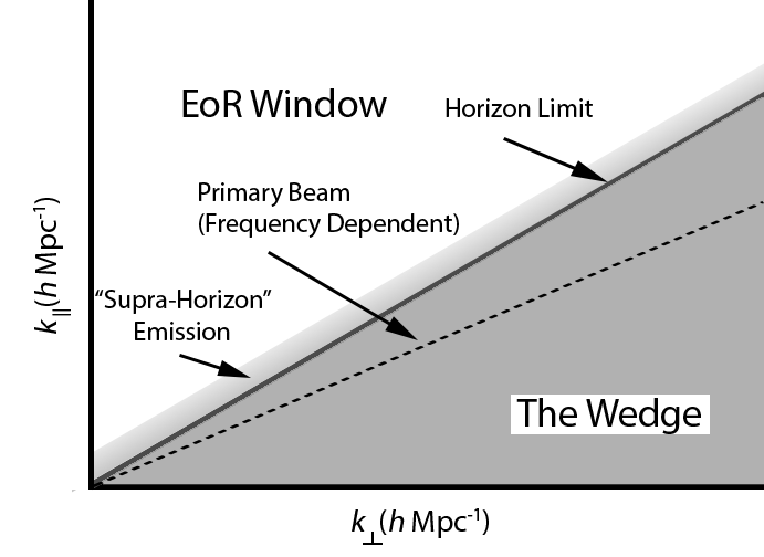
Figure 2.— A schematic diagram of the wedge and EoR window in 2D $k$-space. See §2.2 for explanations of the terms.

Power spectrum analysis in both Dillon et al. (2013b) and Pober et al. (2013a) reveal the presence of the wedge in actual observations. The single-baseline approach (Parsons et al., 2012b) used in Pober et al. (2013a) yields a cleaner EoR window, although at the loss of some sensitivity that comes from combining non-redundant baselines.

However, there is still considerable debate about where to define the “edge” of the wedge. Our three foreground models — summarized in Table 1 — differ in their choice of “wedge edge.” Our pessimistic model also explores the possibility that systematic effects discussed in Hazelton et al. (2013) could prevent to coherent addition of partially redundant baselines. It should be noted that although we use the shorthand “foreground model” to describe these three scenarios, in many ways these represent foreground removal models, since they pertain to improvements over current analysis techniques that may better separate foreground emission from the 21 cm signal.

2.2.1 Foreground Removal Models

At present, observational limits on the “edge” to the foreground wedge in cylindrical $(k_{\perp},k_{\parallel})$-space are still somewhat unclear. Pober et al. (2013a) find the wedge to extend as much as $\Delta k_{\parallel}=0.05\mbox{--}0.1~{}h{\rm Mpc}^{-1}$ beyond the “horizon limit,” i.e., the $k_{\parallel}$ mode on a given baseline that corresponds to the chromatic sine wave created by a flat-spectrum source of emission located at the horizon. (This mode in many ways represents a fundamental limit, as the interference pattern cannot oscillate any faster for a flat-spectrum source of celestial emission; see Parsons et al. 2012b for a full discussion of the wedge in the language of geometric delay space.) Mathematically, the horizon limit is:

$$k_{\parallel,\rm{hor}}=\frac{2\pi}{Y}\frac{|\vec{b}|}{c}=\left(\frac{1}{\nu}\frac{X}{Y}\right)k_{\perp},$$ (2)

where $|\vec{b}|$ is the baseline length in meters, $c$ is the speed of light, $\nu$ is observing frequency, and $X$ and $Y$ are the previously described cosmological scalars for converting observed bandwidths and solid angles to $h{\rm Mpc}^{-1}$, respectively, defined in Parsons et al. (2012a) and Furlanetto et al. (2006b). Pober et al. (2013a) attribute the presence of “supra-horizon” emission — emission at $k_{\parallel}$ values greater than the horizon limit — to spectral structure in the foregrounds themselves, which creates a convolving kernel in $k$-space. Parsons et al. (2012b) predict that the wedge could extend as much as $\Delta k_{\parallel}=0.15~{}h{\rm Mpc}^{-1}$ beyond the horizon limit at the level of the 21 cm EoR signal. This supra-horizon emission has a dramatic effect on the size of the EoR window, increasing the $k_{\parallel}$ extent of the wedge by nearly a factor of 4 on the $16\lambda$-baselines used by PAPER in Parsons et al. (2013).

Others have argued that the wedge will extend not to the horizon limit, but only to the edges of the field-of-view, outside of which emission is too attenuated to corrupt the 21 cm signal. If achievable, this smaller wedge has a dramatic effect on sensitivity, since theoretical considerations suggest that signal-to-noise decreases quickly with increasing $k_{\perp}$ and $k_{\parallel}$. If one compares the sensitivity predictions in Parsons et al. (2012b) for PAPER-132 and Beardsley et al. (2013) for MWA-128 (two comparably sized arrays), one finds that these two different wedge definitions account for a large portion of the difference between a marginal $2\sigma$ EoR detection and a 14$\sigma$ one.

While clearly inconsistent with the current results in Pober et al. (2013a), such a small wedge may be achievable with new advances in foreground subtraction. A large literature of work has gone into studying the removal of foreground emission from 21 cm data (e.g. Morales et al. 2006, Bowman et al. 2009, Liu et al. 2009, Liu & Tegmark 2011, Chapman et al. 2012, Dillon et al. 2013a, Chapman et al. 2013). If successful, these techniques offer the promise of working within the wedge. However, despite the huge sensitivity boost, working within the wedge clearly presents additional challenges beyond simply working within the EoR window. Working within the EoR window requires only keeping foreground leakage from within the wedge to a level below the 21 cm signal; the calibration challenge for this task can be significantly reduced by techniques which are allowed to remove EoR signal from within the wedge (Parsons et al., 2013). Working within the wedge requires foreground removal with up to 1 part in $10^{10}$ accuracy (in mK²) while leaving the 21 cm signal unaffected. Ensuring that calibration errors do not introduce covariance between modes is potentially an even more difficult task. Therefore, given the additional effort it will take to be convinced that a residual excess of power post-foreground subtraction can be attributed to the EoR, it seems plausible that the first robust detection and measurements of the 21 cm EoR signal will come from modes outside the wedge.

To further complicate the issue, several effects have been identified which can scatter power from the wedge into the EoR window. Moore et al. (2013) demonstrate how combining redundant visibilities without image plane correction (as done by PAPER) can corrupt the EoR signal outside the wedge, due to the effects of instrumental polarization leakage. Moore et al. (2013) predict a level of contamination based on simulations of the polarized point source population at low frequencies. Although this predicted level of contamination may already be ruled out by measurements from Bernardi et al. (2013), these effects are a real concern for 21 cm EoR experiments. In the present analysis, however, we do not consider this contamination; rather, we assume that the dense $uv$ coverage of our concept array will allow for precision calibration and image-based primary beam correction not possible with the sparse PAPER array. Through careful and concerted effort this systematic should be able to be reduced to below the EoR level.

As discussed in §2.1.1, we do consider the “multi-baseline mode mixing” effects presented in Hazelton et al. (2013). These effects may result when partially coherent baselines are combined to improve power spectrum sensitivity, introducing additional spectral structure in the foregrounds and thus complicating their mitigation. Conversely, the fact that only instantaneously redundant baselines were combined in Pober et al. (2013a) and Parsons et al. (2013) was partially responsible for the clear separation between the wedge and EoR window. Since recent, competitive upper limits were set using this conservative approach, we include it as our “pessimistic” foreground strategy, noting that recent progress in accounting for the subtleties in partially coherent analyses (Hazelton et al., 2013) make it likely that better schemes will be available soon.

To encompass all these uncertainties in the foreground emission and foreground removal techniques, we use three models for our foregrounds, which we refer to in shorthand as “pessimistic,” “moderate,” and “optimistic”. These models are summarized in Table 1.

Model	Parameters
Moderate	Foreground wedge extends $0.1\ h{\rm Mpc}^{-1}$ beyond horizon limit
Pessimistic	Foreground wedge extends $0.1\ h{\rm Mpc}^{-1}$ beyond horizon limit, and only instantaneously redundant baselines can be combined coherently
Optimistic	Foreground wedge extends to FWHM of primary beam

Table 1Summary of the three foreground removal models.

The “moderate” model is chosen to closely mirror the predictions and data from PAPER. In this model the wedge is considered to extend $\Delta k_{\parallel}=0.1\ h{\rm Mpc}^{-1}$ beyond the horizon limit. The exact scale of the “horizon+.1” limit to the wedge is motivated by the predictions of Parsons et al. (2012b) and the measurements of Pober et al. (2013a) and Parsons et al. (2013). Although the exact extent of the “supra-horizon” emission (i.e. the “+.1”) at the level of the EoR signal remains to be determined, all of these constraints point to a range of 0.05 to 0.15 $h\rm{Mpc}^{-1}$. The uncertainty in this value does not have a large effect on the ultimate power spectrum sensitivity of next generation measurements. For shorthand, we will sometimes refer this model as having a “horizon wedge.”

The “pessimistic” model uses the same horizon wedge as the moderate model, but assumes that only instantaneously redundant baselines are coherently combined. Any non-redundant baselines which sample the same $uv$ pixel as another baseline — either through being similar in length and orientation or through the effects of earth rotation — are added incoherently. In effect, this model covers the case where the multi-baseline mode-mixing of Hazelton et al. (2013) cannot be corrected for. Significant efforts are underway to develop pipelines which correct for this effect and recover the sensitivity boost of partial coherence; since these algorithms have yet to be demonstrated on actual observations, however, we consider this our pessimistic scenario.

The final “optimistic” model, assumes the EoR window remains workable down to $k_{\parallel}$ modes bounded by the FWHM of the primary beam, as opposed to the horizon: $k_{\parallel,\rm{pb}}=\sin(\rm{FWHM}/2)\times k_{\parallel,\rm{hor}}$. The specific choice of the FWHM is somewhat arbitrary; one could also consider a wedge extending the first-null in the primary beam (although this is ill-defined for a Gaussian beam model). Alternatively, one might envision a “no wedge” model meant to mirror the case where foreground removal techniques work optimally, removing all foreground contamination down to the intrinsic spectral structure of the foreground emission. In practice, the small $\sim 10^{\circ}$ size of the HERA primary beam renders these different choices effectively indistinguishable. Therefore, our choice of the primary beam FWHM can also be considered representative of nearly all cases where foreground removal proves highly effective. As of the writing of this paper, no foreground removal algorithms have proven successful to these levels, although this is admittedly a somewhat tautological statement, since no published measurements have reached the sensitivity level of an EoR detection. Furthermore, the sampling point-spread function (PSF) in $k$-space at low $k$’s is expected to make clean, unambiguous retrieval of these modes exceedingly difficult (Liu & Tegmark, 2011; Parsons et al., 2012b), although the small size of the HERA primary beam ameliorates this problem by limiting the scale of this PSF. We find this effect to represent a small ($\lesssim 5\%$) correction to the low-$k$ sensitivities reported in this work. In effect, the optimistic model is included to both show the effects of foregrounds on the recovery of the 21 cm power spectrum, and to give an impression of what could be achievable. For shorthand, this model will be referred to as having a “primary beam wedge.”

Incorporating these foreground models into the sensitivity calculations described in §2.1 is quite straightforward. Modes deemed “corrupted” by foregrounds according to a model are simply excluded from the 3D $k$-space cube, and therefore contribute no sensitivity to the resultant power spectrum measurements.

2.3. Reionization

In order to encompass the large theoretical uncertainties in the cosmic reionization history, we use the publicly available 21cmFAST code v1.01 (Mesinger & Furlanetto, 2007; Mesinger et al., 2011). This semi-numerical code allows us to quickly generate large-scale simulations of the ionization field (400 Mpc on a side) while varying key parameters to examine the possible variations in the 21 cm signal. Following Mesinger et al. (2012), we choose three key parameters to encompass the maximum variation in the signal:

1. $\zeta$, the ionizing efficiency: $\zeta$ is a conglomeration of a number of parameters relating to the amount of ionizing photons escaping from high-redshift galaxies: $f_{\rm esc}$, the fraction of ionizing photons which escape into the IGM, $f_{*}$, the star formation efficiency, $N_{\gamma}$, the number of ionizing photons produced per baryon in stars, and $n_{\rm rec}$ the average number of recombinations per baryon. Rather than parameterize the uncertainty in these quantities individually, it is common to define $\zeta=f_{\rm esc}f_{*}N_{\gamma}/(1+n_{\rm rec})$ (Furlanetto et al., 2004). We explore a range of $\zeta=10-50$ in this work, which is generally consistent with current CMB and Ly$\alpha$ constraints on reionization (Mesinger et al., 2012).

2. $T_{\rm vir}$, the minimum virial temperature of halos producing ionizing photons: $T_{\rm vir}$ parameterizes the mass of the halos responsible for reionization. Typically, $T_{\rm vir}$ is chosen to be $10^{4}$ K, which corresponds to a halo mass of $10^{8}~{}\rm{M}_{\odot}$ at $z=10.$ This value is chosen because it represents the temperature at which atomic cooling becomes efficient. In this work, we explore $T_{\rm vir}$ ranging from $10^{3}\mbox{--}3\times 10^{5}$ K to span the uncertainty in high-redshift galaxy formation physics as to which halos host significant stellar populations (see e.g. Haiman et al. 1996, Abel et al. 2002 and Bromm et al. 2002 for lower mass limits on star-forming halos, and e.g. Mesinger & Dijkstra 2008 and Okamoto et al. 2008 for feedback effects which can suppress low mass halo star formation).

3. $R_{\rm mfp}$, the mean free path of ionizing photons through the intergalactic medium (IGM): $R_{\rm mfp}$ sets the maximum size of HII regions that can form during reionization. Physically, it is set by the space density of Lyman limit systems, which act as sinks of ionizing photons. In this work, we explore a range of mean free paths from 3 to 80 Mpc, spanning the uncertainties in current measurements of the mean free path at $z\sim 6$ (Songaila & Cowie, 2010).

We note there are many other tunable parameters that could affect the reionization history. In particular, the largest 21 cm signals can be produced in models where the IGM is quite cold during reionization (cf. Parsons et al. 2013). We do not include such a model here, and rather focus on the potential uncertainties within “vanilla” reionization; for an analysis of the detectability of early epochs of X-ray heating, see Christian & Loeb (2013) and Mesinger et al. (2013). Also note that 21cmFAST assumes the values of the EoR parameters are constant over all redshifts considered. With the exception of our three EoR variables, we use the fiducial parameters of the 21cmFAST code; see Mesinger et al. (2011) for more details.

Note we do assume that $T_{\rm spin}\gg T_{\rm CMB}$ at all epochs, which could potentially create a brighter signal at the highest redshifts. Given that thermal noise generally dominates the signal at the highest redshifts regardless, we choose to ignore this effect, noting that it will only increase the difficulties of $z>10$ observations we describe below. (Although this situation may be changed by the alternate X-ray heating scenarios considered in Mesinger et al. 2013.)

2.3.1 “Vanilla” Model

For the sake of comparison, it is worthwhile to have one fiducial model with “middle-ground” values for all the parameters in question. We refer to this model as our “vanilla” model. Note that this model was not chosen because we believe it most faithfully represents the true reionization history of the universe (though it is consistent with current observations). Rather, it is simply a useful point of comparison for all the other realizations of the reionization history. In this model, the values of the three parameters being studied are $\zeta=31.5,\ T_{\rm vir}=1.5\times 10^{4}~{}\rm{K}$ and $R_{\rm mfp}=30~{}\rm{Mpc}$. This model achieves 50% ionization at $z\sim 9.5$, and complete ionization at $z\sim 7$. The redshift evolution of the power spectrum in this model is shown in Figure 3.

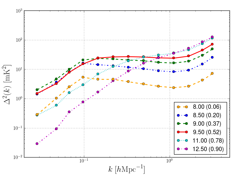
Figure 3.— Power spectra at several redshifts for our vanilla reionization model with $\zeta=31.5,\ T_{\rm vir}=1.5\times 10^{4}~{}\rm{K},$ and $R_{\rm mfp}=30~{}\rm{Mpc}$. Numbers in parentheses give the neutral fraction at that redshift.

2.3.2 The Effect of the Varying the EoR Parameters

The effects of varying $\zeta$, $T_{\rm vir}$ and $R_{\rm mfp}$ are illustrated in Figure 4.

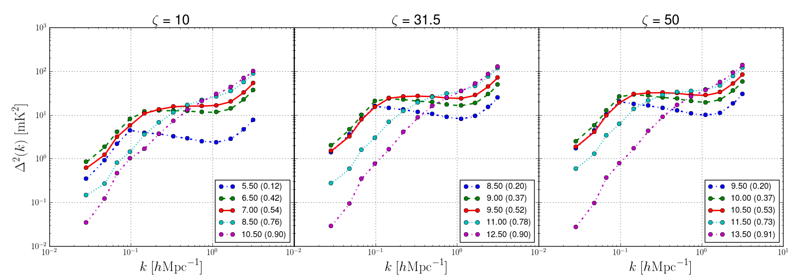
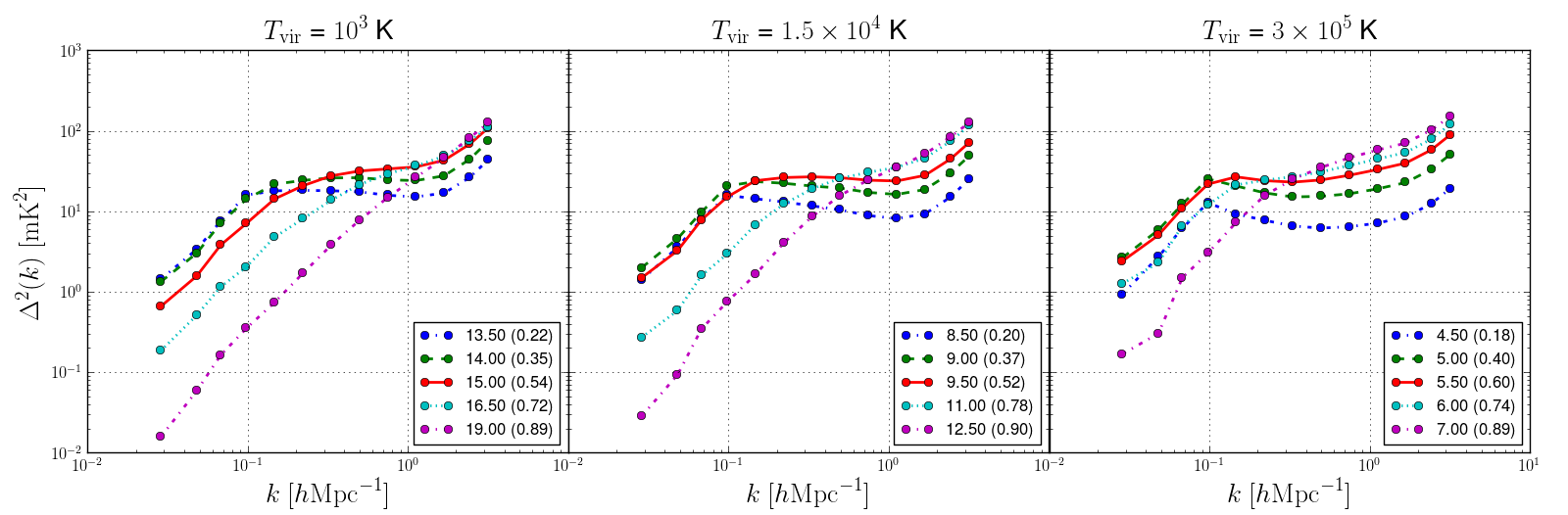
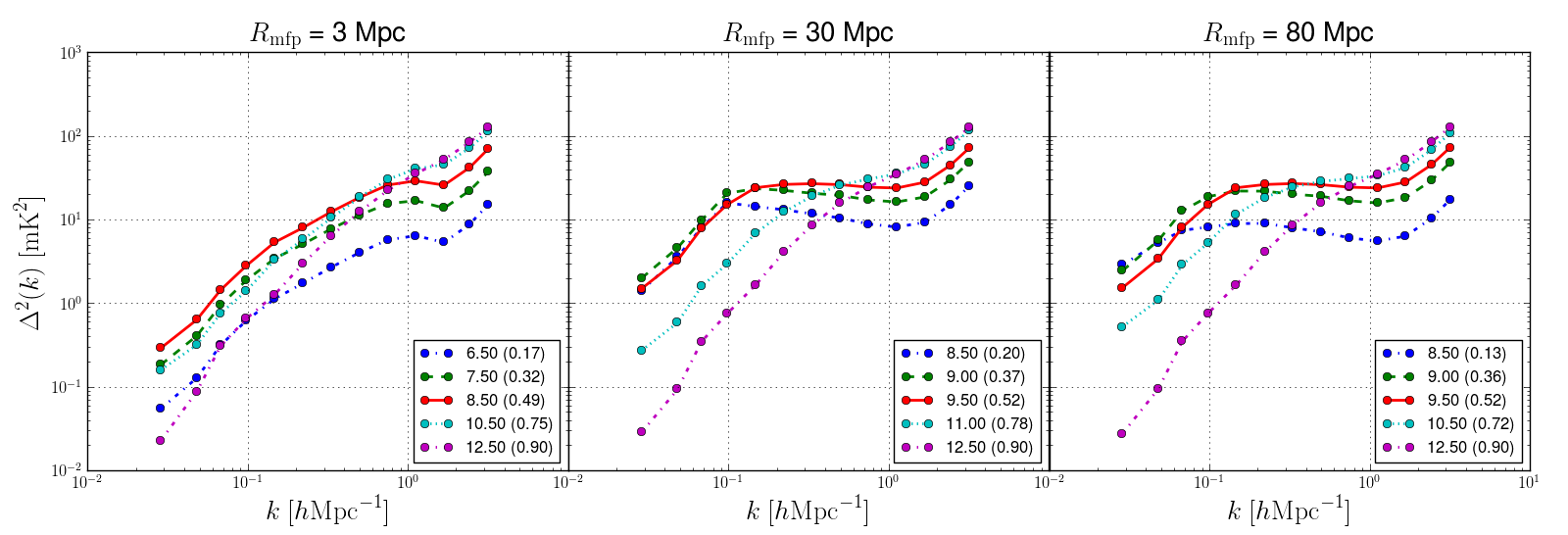
Figure 4.— Power spectra as a function of redshift for the low, high, and fiducial values of the ionizing efficiency, $\zeta$ (top row), $T_{\rm vir}$ (middle row) and $R_{\rm mfp}$ (bottom row). Exact values of each parameter are given in the panel title. Numbers in parentheses give the neutral fraction at that redshift. The central panel is the vanilla model and is identical to Figure 3 (although the $z=8$ curve is not included for clarity). Colors in each panel map to roughly the same neutral fraction. Qualitative effects of varying each parameter are apparent: $\zeta$ changes the timing of reionization but not the shape of the power spectrum; $T_{\rm vir}$ drastically alters the timing of reionization with smaller effects on the power spectrum shape; and small values of $R_{\rm mfp}$ reduce the amount of low $k$ power.

Each row shows the effect of varying one of the three parameters while holding the other two fixed. The middle panel in each row is for our vanilla model, and thus is the same as Figure 3 (although the $z=8$ curve is not included for clarity). Several qualitative observations can immediately be made. Firstly, we can see from the top row that $\zeta$ does not significantly change the shape of the power spectrum, but only the duration and timing of reionization. This is expected, since the same sources are responsible for driving reionization regardless of $\zeta$. Rather, it is only the number of ionizing photons that these sources produce that varies.

Secondly, we can see from the middle row that the most dramatic effect of $T_{\rm vir}$ is to substantially change the timing of reionization. Our high and low values of $T_{\rm vir}$ create reionization histories that are inconsistent with current constraints from the CMB and Ly$\alpha$ forest (Fan et al., 2006; Hinshaw et al., 2012). This alone does not rule out these values of $T_{\rm vir}$ for the minimum mass of reionization galaxies, but it does mean that some additional parameter would have to be adjusted within our vanilla model to create reasonable reionization histories. We can also see that the halo virial temperature affects the shape of the power spectrum. When the most massive halos are responsible for reionization, we see significantly more power on very large scales than in the case where low-mass galaxies reionize the universe.

Finally, the bottom row shows that the mean free path of ionizing photons also affects the amount of large scale power in the 21 cm power spectrum. $R_{\rm mfp}$ values of 30 and 80 Mpc produce essentially indistinguishable power spectra, except at the very largest scales at late times. However, the very small value of $R_{\rm mfp}$ completely changes the shape of the power spectrum, resulting in a steep slope versus $k$, even at 50% ionization, where most models show a fairly flat power spectrum up to a “knee” feature on larger scales. In section 3.4, we consider using some of these characteristic features to qualitatively assess properties from reionization in 21 cm measurements.

3. Results

In this section, we will present the predicted sensitivities that result from combinations of EoR and foreground models. We will focus predominantly on the moderate model where one can take advantage of partially-redundant baselines, but the wedge still contaminates $k_{\parallel}$ modes below $0.1~{}h\rm{Mpc}^{-1}$ above the horizon limit.‘ In presenting the sensitivity levels achievable under the other two foreground models, we focus on the additional science that will be prevented/allowed if these models represent the state of foreground removal analysis.

We will take several fairly orthogonal approaches towards understanding the science that will be achievable. First, in §3.1, our approach is to attempt to cover the broadest range of possible power spectrum shapes and amplitudes in order to make generic conclusions about the detectability of the 21 cm power spectrum. In §3.2, §3.3, and §3.4, we focus on our vanilla reionization model and semi-quantitatively explore the physical lessons the predicted sensitivities will permit. Finally, in §3.5, we undertake a Fisher matrix analysis and focus on specific determinations of EoR parameters with respect to the fiducial evolution of our vanilla model, exploring the degeneracies between parameters and providing lessons in how to break them. The end result of these various analyses is a holistic picture about the kinds of information we can derive from next generation EoR measurements.

3.1. Sensitivity Limits

In this section, we consider the signal-to-noise ratio of power spectrum measurements achievable under our various foreground removal models. The main results are presented in Figures 5, 6, 7, and 8. Figure 5 shows the constraints on the 50% ionization power spectrum in our vanilla model for each of the three foreground models, as well as the measurement significances of alternate ionization histories using the vanilla model. Figures 6, 7, and 8 show the power spectrum measurement signifances that result when the EoR parameters are varied for the moderate, pessimistic, and optimistic foreground models respectively.

3.1.1 Methodology

In order to explore the largest range of possible power spectrum shapes and amplitudes, it is important to keep in mind the small but non-negligible spread between various theoretical predictions in the literature. To avoid having to run excessive numbers of simulations, we make use of the observation that much of the differences between simulations is due to discrepancies in their predictions for the ionization history $x_{\textrm{HI}}(z)$, in the sense that the differences decrease if neutral fraction (rather than redshift) is used as the time coordinate for cross-simulation comparisons. We thus make the ansatz that given a single set of parameters $(\zeta,T_{\rm vir},R_{\rm mfp})$, the 21cmFAST power spectrum outputs can (modulo an overall normalization factor) be translated in redshift to mimic the outputs of alternative models that predict a different ionization history. In practice, the 21cmFAST simulation provides a suite of power spectra in either (a) fixed steps in $z$ or (b) approximately fixed steps in $x_{\rm HI}$, but constrained to appear at a single $z$. We utilize the latter set, and “extrapolate” each neutral fraction to a variety of redshifts by scaling the amplitude with the square of the mean temperature of the IGM as $(1+z)$, as anticipated when ionization fractions dominate the power spectrum (McQuinn et al., 2006; Lidz et al., 2008). While not completely motivated by the physics of the problem (since within 21cmFAST a given set of EoR parameters does produce only one reionization history), this approach allows us to explore an extremely wide range of power spectrum amplitudes while running a reasonable number of simulations.

3.1.2 Moderate Foreground Model

Figure 5 shows forecasts for constraints on our fiducial reionization model under the three foreground scenarios.

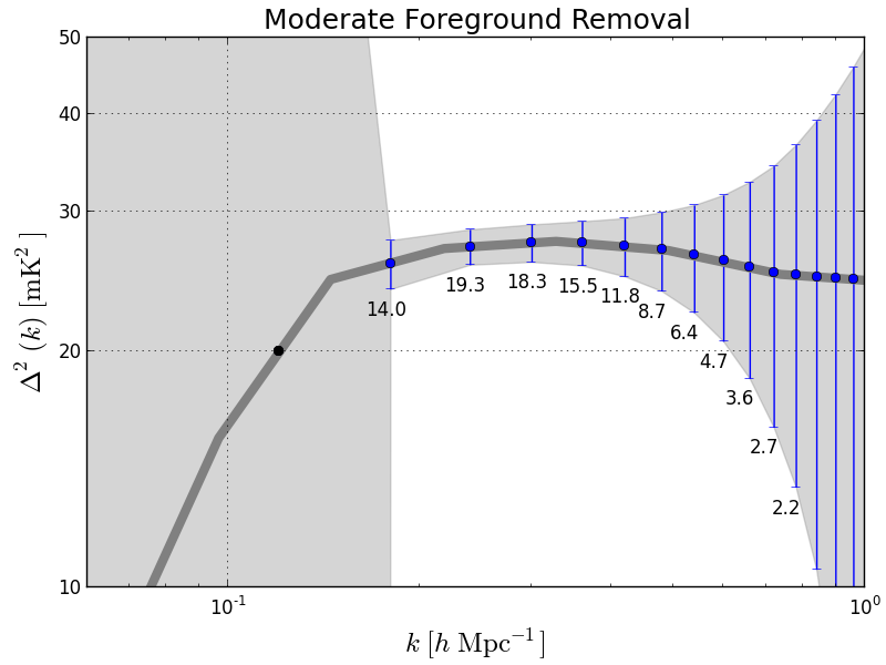
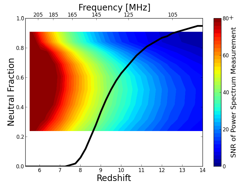
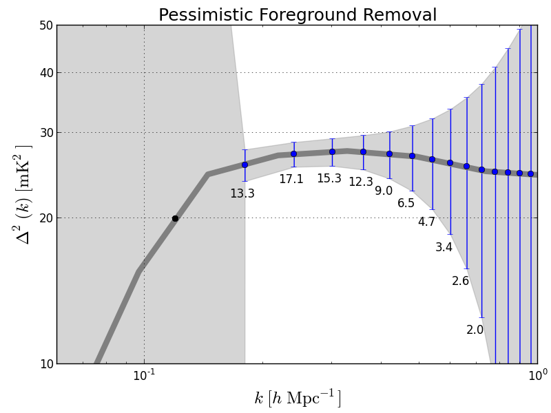
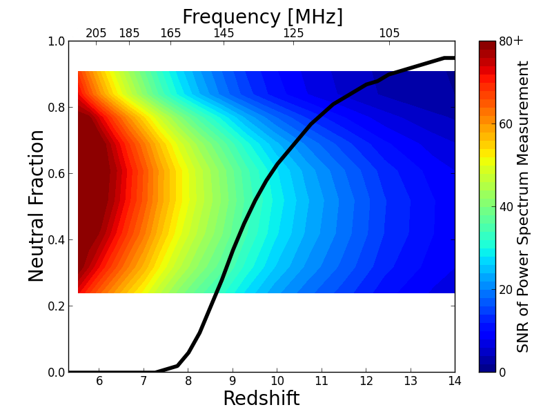
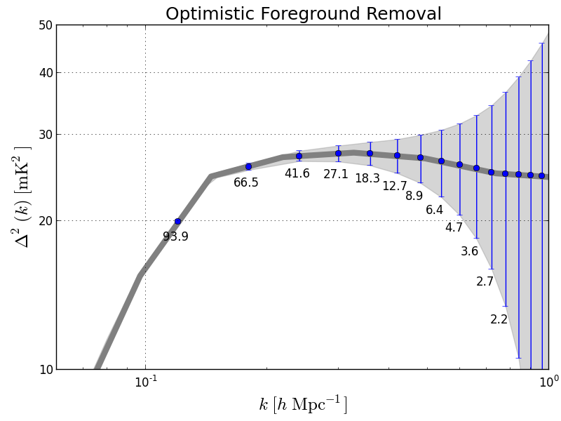
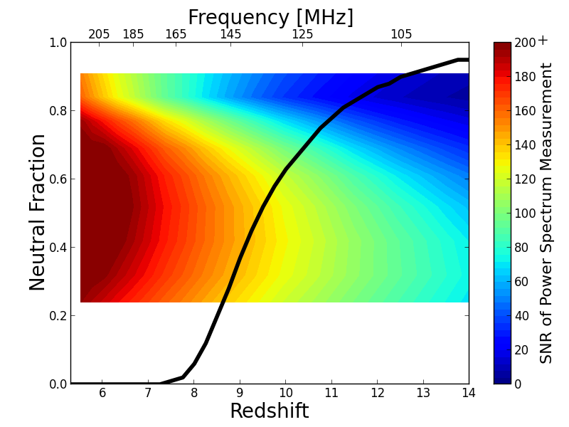
Figure 5.— Left: Power spectrum constraints on the fiducial EoR model at $z=9.5\ (53\%$ ionization) for each of the three foreground removal models: moderate (top), pessimistic (middle) and optimistic (bottom). The shaded gray region shows the $1\sigma$ error range, whereas the location of the blue error bars indicate the binned sampling pattern; the binning is set by the bandwidth of 8 MHz. Black points without error bars indicate measurements allowed by instrumental parameters, but rendered unusable according to the foreground model. The net result of these measurements are $38\sigma$, $32\sigma$, and $133\sigma$ detections of the fiducial power spectrum for the moderate, pessimistic and optimistic models, respectively. Individual numbers below each error bar indicate the significance of the measurement in that bin. Right: Colored contours show the total SNR of a power spectrum detection as a function of redshift and neutral fraction for the three foreground removal models: moderate (top), pessimistic (middle) and optimistic (bottom). The black curve shows the fiducial evolution of the vanilla model; contour values off of the black curve are obtained by translating the fiducial model in redshift. This figure therefore allows one to examine the SNR for a far broader range of reionization histories than only those predicted by simulations with vanilla model parameters. Alternative evolution histories are less physically motivated, since a given set of EoR parameters does only predict one evolution history. The plotted sensitivities assume 8 MHz bandwidths are used to measure the power spectra, so not all points in the horizontal direction are independent. The incomplete coverage versus $x_{\rm HI}$ does not indicate that measurements cannot be made at these neutral fractions; rather, it is a feature of the 21cmFAST code, and is explained in §3.1.

The left-hand panels of the figure show the constraints on the spherically averaged power spectrum at $z=9.5$, the point of 50% ionization in this model, for the three foreground removal models. (The 50% ionization point generally corresponds to the peak power spectrum brightness at the scales of interest — as can be seen in Figure 4 — making its detection a key goal of reionization experiments (Lidz et al., 2008; Bittner & Loeb, 2011).) For the moderate model (top row), the errors amount to a $38\sigma$ detection of the 21 cm power spectrum at 50% ionization.

The right-hand panels of Figure 5 warrant somewhat detailed explanation. The three rows again correspond to the three foreground removal models. In each panel, the horizontal axis shows redshift and the vertical axis shows neutral fraction; thus this space spans a wide range of possible reionization histories. The black curve is the evolution of the vanilla model through this space. The colored contours show the signal-to-noise ratio of a HERA measurement of the 21 cm power spectrum at that point in redshift/neutral fraction space, where the power spectrum of a given $x_{\rm HI}$ is extrapolated in redshift space as described in the beginning of §3.1. The colorscale is set to saturate at different values in each row: $80\sigma$ (moderate and pessimistic) and $200\sigma$ (optimistic). These sensitivities assume 8 MHz bandwidths are used to measure the power spectra, so not every value on the redshift-axis can be taken as an independent measurement. The non-uniform coverage versus ionization fraction (i.e. the white space at high and low values of $x_{\rm HI}$) — which appears with different values in the panels of Figures 5, 6, 7, and 8 — is a feature of the 21cmFAST code when attempting to produce power spectra for a set of input parameters at relatively even spaced values of ionization fraction. The black line is able to extend into the white region because it was generated to have uniform spacing in $z$ as opposed to $x_{\rm HI}$. The fact that these values are missing has minimal impact on the conclusions drawn in this work.

In the moderate model, the 50% ionization point of the fiducial power spectrum evolution is detected at $\sim 40\sigma$. However, we see that nearly every ionization fraction below $z\sim 9$ is detected with equally high significance. In general, the contours follow nearly vertical lines through this space. This implies that the evolution of sensitivity as a function of redshift (which is primarily driven by the system temperature) is much stronger than the evolution of power spectrum amplitude as a function of neutral fraction (which is primarily driven by reionization physics).

Figure 6 shows signal-to-noise contour plots for six different variations of our EoR parameters, using only the moderate foreground scenario. (The pessimistic and optimistic equivalents of this figure are shown in Figures 7 and 8, respectively.)

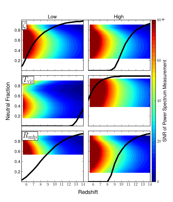
Figure 6.— Signal-to-noise ratio of 21 cm power spectrum detections under the moderate foreground scenario for the high and low values of the parameters in our EoR models as functions of neutral fraction and redshift. In each panel, one parameter is varied, while the other two are held fixed at the “vanilla” values. The black curve shows the fiducial evolution for that set of model parameters. The incomplete coverage versus $x_{\rm HI}$ does not indicate that measurements cannot be made at these neutral fractions; rather, it is a feature of the 21cmFAST code, and is explained in §3.1. Top: the ionizing efficiency, $\zeta$. Values are $\zeta=10$ (left) and $\zeta=50$ (right). Middle: the minimum virial temperature of ionizing haloes, $T_{\rm vir}$. Values are $T_{\rm vir}=1\times 10^{3}$ K (left) and $T_{\rm vir}=3\times 10^{5}$ K (right). Bottom: the mean free path for ionizing photons through the IGM, $R_{\rm mfp}$. Values are $R_{\rm mfp}=3$ Mpc (left) and $R_{\rm mfp}=80$ Mpc (right). The moderate foreground removal scenario generically allows for a high significance measurement for nearly any reasonable reionization history.

In each panel, we have varied one parameter from the fiducial vanilla model. In particular, we choose the lowest and highest values of each parameter considered in §2.3. Since we extrapolate each power spectrum to a wide variety of redshifts, choosing only the minimum and maximum values leads to little loss of generality. Rather, we are picking extreme shapes and amplitudes for the power spectrum, and asking whether they can be detected if such a power spectrum were to correspond to a particular redshift. And, as with the vanilla model shown in Figure 5, it is clear that the moderate foreground removal scenario allows for the 21 cm power spectrum to be detected with very high significance below $z\sim 8-10$, depending on the EoR model. Relative to the effects of system temperature, then, the actual brightness of the power spectrum as a function of neutral fraction plays a small role in determining the detectability of the cosmic signal. Of course, there is still a wide variety of power spectrum brightnesses; for a given EoR model, however, the relative power spectrum amplitude evolution as a function of redshift is fairly small.

There are also several more specific points about Figure 6 that warrant comment. Firstly, as stated in §2.3.2, the ionizing efficiency $\zeta$ has little effect on the shape of the power spectrum, but only on the timing and duration of reionization. This is clear from the identical sensitivity levels for both values of $\zeta$, as well as for the vanilla model shown in Figure 5. Secondly, we reiterate that by tuning values of $T_{\rm vir}$ alone, we can produce ionization histories that are inconsistent with observations of the CMB and Lyman-$\alpha$ forest. In our analysis here, we extrapolate the power spectrum shapes produced by these extreme histories to more reasonable redshifts to show the widest range of possible scenarios. The fact that the fiducial evolution histories (black lines) of the $T_{\rm vir}$ row are wholly unreasonable is understood, and does not constitute an argument against this type of analysis.

3.1.3 Other Foreground Models

It is clear then, that the moderate foreground removal scenario will permit high sensitivity measurements of the 21 cm power with the next generation of experiments. Before considering what types of science these sensitivities will enable, it is worthwhile to consider the effects of the other foreground removal scenarios.

Our pessimistic scenario assumes — like the moderate scenario — that foregrounds irreparably corrupt $k_{\parallel}$ modes within the horizon limit plus $0.1~{}h{\rm Mpc}^{-1}$, but also conservatively omits the coherent addition of partially redundant baselines in an effort to avoid multi-baseline systematics. As stated, this is the most conservative foreground case we consider. The achievable constraints on our fiducial vanilla power spectrum under this model were shown in the second row of Figure 5; Figure 7 shows the sensitivities for other EoR models.

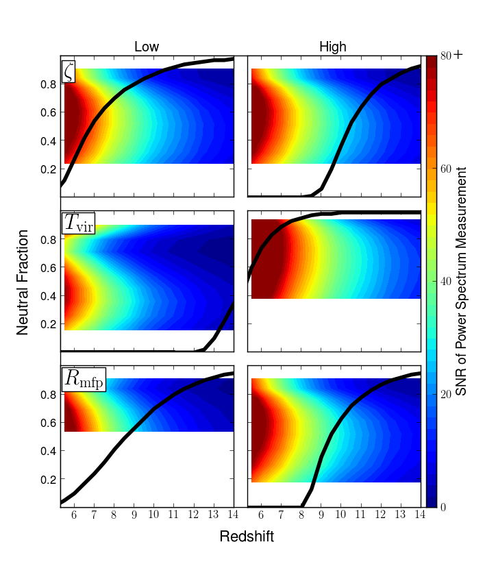
Figure 7.— Same as Figure 6, but for the pessimistic foreground model. Note that the color-scale is the same as Figure 6 and saturates at $80\sigma$.

The sensitivity loss associated with coherently adding only instantaneously redundant baselines is fairly small, $\sim 20\%$. It should be noted that this pessimistic model affects only the thermal noise error bars relative to the moderate model; sample variance contributes the same amount of uncertainty in each bin. In an extreme sample variance limited case, the pessimistic and moderate models would yield the same power spectrum sensitivities. We will further explore the contribution of sample variance to these measurements in §3.3. Here we note that the pessimistic model generally increases the thermal noise uncertainties by $30\mbox{--}40\%$ over the moderate model. This effect will be greater for an array with less instantaneous redundancy than the HERA concept design.

Finally, the sensitivity to the vanilla EoR model under the optimistic foreground removal scenario is shown in the bottom row of Figure 5. Figure 8 shows the sensitivity results for the other EoR scenarios.

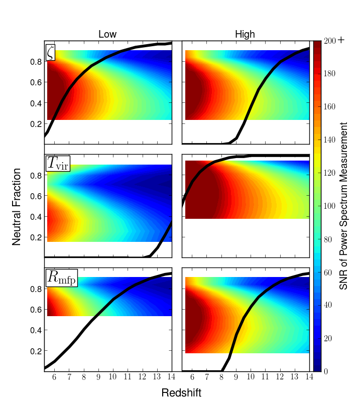
Figure 8.— Same as Figures 6 and 7, but for the optimistic foreground model. Note that the color-scale has changed to saturate at $200\sigma$.

The sensitivities for the optimistic model are exceedingly high. Comparison of the top and bottom rows of Figure 5 shows that this model does not uniformly increase sensitivity across $k$-space, but rather the gains are entirely at low $k$s. This behavior is expected, since the effect of the optimistic model is to recover large scale modes that are treated as foreground contaminated in the other models. The sensitivity boosts come from the fact that thermal noise is very low at these large scales, since noise scales as $k^{3}$ while the cosmological signal remains relatively flat in $\Delta^{2}(k)$ space. We consider the effect of sample variance in these modes in §3.3.

3.2. The Timing and Duration of Reionization

One of the first key parameters that is expected from 21 cm measurement of the EoR power spectrum is the redshift at which the universe was 50% ionized, sometimes referred to as “peak reionization.” The rationale behind this expectation is evident from Figure 4, where the power spectrum generically achieves peak brightness at $k\sim 0.1~{}h{\rm Mpc}^{-1}$ for $x_{\rm HI}=0.5$. However, given the steep increase of $T_{\rm sys}$, one must ask if an experiment will truly have the sensitivity to distinguish the power spectrum at $z_{\rm peak}$ from those on either side. Figure 9 shows the error bars on our fiducial power spectrum model at 50% ionization ($z=9.5$), as well as those on the neighboring redshifts $z=8.5$ and $z=10.5$, under each of our three foreground models. In both the pessimistic and moderate models (left and middle panel), the $z=8.5$ (20% neutral), $z=9.5$ (52% neutral) and $z=10.5$ (71% neutral) are distinguishable at the few sigma level. This analysis therefore suggests that it should be possible to identify peak reionization to within a $\Delta z\sim 1$, with a strong dependence on the actual redshift of reionization (since noise is significantly lower at lower redshifts).

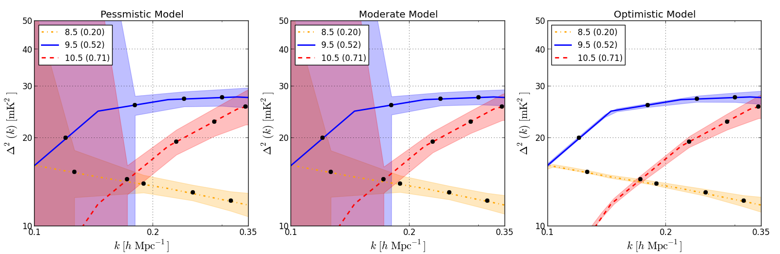
Figure 9.— $1\sigma$ uncertainties in the measurements of the fiducial EoR power spectrum at redshifts 8.5, 9.5 and 10.5, corresponding to neutral fractions of 0.20, 0.52 and 0.71, respectively. Different panels show the results for the different foreground models: pessimistic (left), moderate (middle), and optimistic (right). The pessimistic and moderate scenarios should both permit measurements of $\Delta z\sim 1.0$. The optimistic scenario will allow for detailed characterization of the power spectrum evolution.

It is worth noting, however, that even relatively high significance detections of the power spectrum ($\gtrsim 5\mbox{--}10\sigma$) may not permit one to distinguish power spectrum of peak reionization from those at nearby redshifts — especially as one looks to higher $z$. For our vanilla EoR model, we find a $\sim 10\sigma$ detection is necessary to distinguish the $z=8.5,\ 9.5,$ and 10.5 power spectra at the $>1\sigma$ level. In fact, for this level of significance, nearly all of the power spectra at redshifts higher than peak reionization at $z=9.5$ are indistinguishable given the steep rise in thermal noise. Even if the current generation of 21 cm telescopes does yield a detection of the 21 cm power spectrum, these first measurements do not guarantee stringent constraints on the peak redshift of reionization.

Finally, one can see that the high sensitivities permitted by the optimistic foreground model will allow a detailed characterization of the power spectrum amplitude and slope as a function of redshift. We discuss exactly what kind of science this will enable (beyond detecting the timing and duration of reionization) in §3.5.

3.3. Sample Variance and Imaging

Given the high power spectrum sensitivities achievable under all of our foreground removal models, one must investigate the contributions of sample variance to the overall errors. For the moderate foreground model, Figure 10 shows the relative contribution of sample variance and thermal noise to the errors shown in the top-left panel of Figure 5.

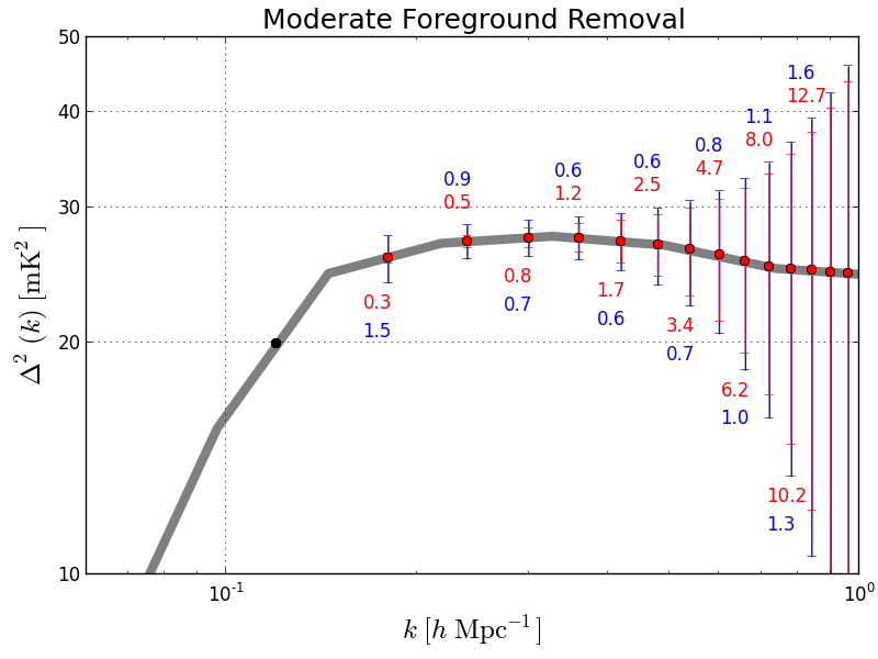
Figure 10.— The breakdown of the error bars in the top-left panel of Figure 5 (vanilla EoR model and moderate foreground removal scenario). Red shows the contribution of thermal noise, blue the contribution of sample variance. The text shows the value of each contribution in mK² — not the significance of the detection, as in previous plots. Regions where the sample variance error dominates the thermal noise error are in the imaging regime. The placement of the numerical values above or below the error bar has no significance; it is only for clarity. Sample variance dominates the errors in the moderate foreground scenario on scales $k<0.25~{}h{\rm Mpc}^{-1}$.

From this plot, it is clear that sample variance contributes over half of the total power spectrum uncertainty on scales $k<0.3h{\rm Mpc}^{-1}$. If the power spectrum constituted the ultimate measurement of reionization, this would be an argument for a survey covering a larger area of sky. For our HERA concept array, which drift-scans, this is not possible, but may be for phased-array designs. However, the sample variance dominated regime is very nearly equivalent to the imaging regime: thermal noise is reduced to the point where individual modes have an SNR $\gtrsim$ 1. Therefore, using a filter to remove the wedge region (e.g. Pober et al. 2013a), a collecting area of $0.1~{}{\rm km}^{2}$ should provide sufficient sensitivity to image the Epoch of Reionization over $\sim 800$ sq. deg. (6 hours of right ascension $\times\ 8.7^{\circ}~{}\rm{FHWM})$ on scales of $0.1\mbox{--}0.25~{}h{\rm Mpc}^{-1}$. We note that the HERA concept design is not necessarily optimized for imaging; other configurations may be better suited if imaging the EoR is the primary science goal.

The effect of the other foreground models on imaging is relatively small. The poorer sensitivities of the pessimistic model push up thermal noise, lowering the highest $k$ that can be imaged to $k\sim 0.2h{\rm Mpc}^{-1}$. The optimistic foreground model recovers significant SNR on the largest scales, to the point where sample variance dominates all scales up to $0.3~{}h{\rm Mpc}^{-1}$. The effects of foregrounds and the wedge on imaging with a HERA-like array will be explored in future work.

3.4. Characteristic Features of EoR Power Spectrum

Past literature has discussed two simple features of the 21 cm power spectra to help distinguish between models: the slope of the power spectrum and the sharp drop in power (the “knee”) on the largest scales (McQuinn et al., 2006). In particular, the mass of the halos driving reionization (parametrized in this analysis by the minimum virial temperature of ionizing halos) should affect the slope of the power spectrum. Since more massive halos are more highly clustered, they should concentrate power on larger scales, yielding a flatter slope. The second row of Figure 4 suggests this effect is small, although not implausible. The knee of the power spectrum at large scales should correspond to the largest ionized bubble size, since there will be little power on scales larger than these bubbles (Furlanetto et al., 2006a). The position of the knee should be highly sensitive to the mean free path for ionizing photons through the IGM, since this sets how large bubbles can grow. This argument is indeed confirmed by the third row of Figure 4, where the smaller values of $R_{\rm mfp}$ lack significant power on large scales compared to those models with larger values. Unfortunately, since our third parameter $\zeta$ does not change the shape of the power spectrum, constraining different values of $\zeta$ will not be possible with only a shape-based analysis. In this section we first extend these qualitative arguments based on salient features in the power spectra, and then present a more quantitative analysis on distinguishing models in §3.5.

To quantify the slope of the power spectrum, we fit a straight line to the predicted power spectrum values between $k=0.1\mbox{--}1.0~{}h{\rm Mpc}^{-1}$. When we refer to measuring the slope, we refer to measuring the slope of this line, given the error bars in the $k$-bins between $0.1\mbox{--}1.0~{}h{\rm Mpc}^{-1}$. This choice of fit is not designed to encompass the full range of information contained in measurements of the power spectrum shape. Rather, the goal of this section is to find simple features of the power spectrum that can potentially teach us about the EoR without resorting to more sophisticated modeling.

Figure 11 shows the evolution of the slope of the linear fit to the power spectrum over the range $k=0.1\mbox{--}1.0~{}h{\rm Mpc}^{-1}$, as a function of neutral fraction for several EoR models.

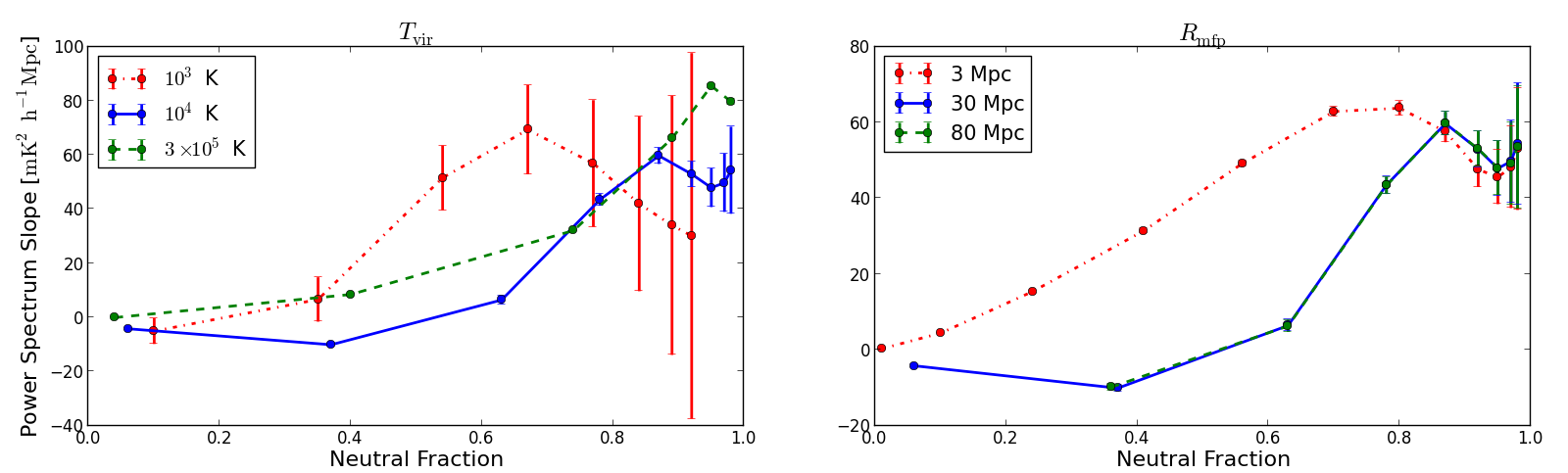
Figure 11.— The power spectrum slope in units of ${\rm mK}^{2}h^{-1}\rm{Mpc}$ between $k=0.1$ and $1.0h{\rm Mpc}^{-1}$ as a function of neutral fraction for various EoR models. Note that error bars are plotted on all points and correspond to the redshift of a given neutral fraction for that model. Left: Different values of $T_{\rm vir}$. Right: Different values of $R_{\rm mfp}$. While different values of $T_{\rm vir}$ and $R_{\rm mfp}$ produce considerable changes in the power spectrum slope, it will be difficult to unambiguously interpret its physical significance.

Error bars in both panels correspond to the error measured under the moderate foreground model for a given neutral fraction in the fiducial history of a model. This means that, e.g., the high neutral fractions in the $T_{\rm vir}=10^{3}$ K curve have thermal noise errors corresponding to $z\sim 20$, outside the range of many proposed experiments. Given that caveat, it does appear that the low-mass ionizing galaxies produce power spectra with significantly steeper slopes at moderate neutral fractions than those models where only high mass galaxies produce ionizing photons. However, it is also clear that small-bubble (i.e. low mean free path) models can yield steep slopes. Therefore, while there may be some physical insight to be gleaned from measuring the slope of the power spectrum and its evolution, even the higher sensitivity measurements permitted by the optimistic foreground model may not be enough to break these degeneracies. In §3.5, we specifically focus on the kind of information necessary to disentangle these effects.

A comparison of the error bars in the moderate and optimistic foreground scenario measurements of the vanilla power spectrum (rows one and three in Figure 5) reveals the difficulty in recovering the position of the knee without foreground subtraction: foreground contamination predominantly affects low $k$ modes, rendering large scale features like the knee inaccessible. In particular, the additive component of the horizon wedge severely restricts the large scale information available to the array. Without probing large scales, confirming the presence (or absence) of a knee feature is likely to be impossible. However, Figure 5 does show that if foreground removal allows for the recovery of these modes, the knee can be detected with very high significance, even the presence of sample variance.

3.5. Quantitative Constraints on Model Parameters

In previous sections, we considered rather large changes to the input parameters of the 21cmFAST model. These gave rise to theoretical power spectra that exhibited large qualitative variations, and encouragingly, we saw that such variations should be easily detectable using next-generation instruments such as HERA. We now turn to what would be a natural next step in data analysis following a broad-brush, qualitative discrimination: a determination of best-fit values for astrophysical parameters. In this section, we forecast the accuracy with which $T_{\textrm{vir}}$, $R_{\textrm{mfp}}$, and $\zeta$ can be measured by a HERA-like instrument, paying special attention to degeneracies. In many of the plots, we will omit the pessimistic foreground scenario, for often the results from it are identical to (and visually indistinguishable from) those from moderate foregrounds. Ultimately, our results will suggest parameter constraints that are smaller than one can justifiably expect given the reasonable, but non-negligible uncertainty surrounding simulations of reionization (Zahn et al., 2011). Our final error bar predictions (which can be found in Table 2) should therefore be interpreted cautiously, but we do expect the qualitative trends in our analysis to continue to hold as theoretical models improve.

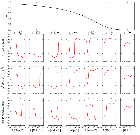
Figure 12.— Power spectrum derivatives as a function of wavenumber $k$ and redshift $z$. Each of the lower three rows shows derivatives with respect to a different parameter in our three-parameter model, and the top panel (aligned in redshift with the bottom panels) shows the corresponding neutral fraction. Because our parameter vector $\boldsymbol{\theta}$ (Equation [3]) contains non-dimensionalized parameters, the derivatives $\partial\Delta^{2}(k,z)/\partial\theta_{i}$ are equivalent (if evaluated at the fiducial parameter values) to the logarithmic derivatives shown here. Note that the derivatives with respect to $\zeta$ and $R_{\textrm{mfp}}$ have been multiplied by $-1$ to facililate later comparisons. The vertical axes for the derivatives are linear between $-10^{-1}$ and $10^{1}$, and are logarithmic outside that range. From this figure, we see that while the lowest redshifts are easy to access observationally, the model parameters are highly degenerate. The higher redshifts are less degenerate, but thermal noise and foregrounds make observations difficult.

3.6. Fisher matrix formalism for errors on model parameters

To make our forecasts, we use the Fisher information matrix $\mathbf{F}$, which takes the form

$$\mathbf{F}_{ij}\equiv-\Big{\langle}\frac{\partial^{2}\ln\mathcal{L}}{\partial\theta_{i}\partial\theta_{j}}\Big{\rangle}=\sum_{k,z}\frac{1}{\varepsilon^{2}(k,z)}\frac{\partial\Delta^{2}(k,z)}{\partial\theta_{i}}\frac{\partial\Delta^{2}(k,z)}{\partial\theta_{j}},$$ (3)

where $\mathcal{L}$ is the likelihood function (i.e. the probability distribution for the measured data as a function of model parameters), $\varepsilon(k,z)$ is the error on $\Delta^{2}(k,z)$ measurements as a function of wavenumber $k$ and redshift $z$, and $\boldsymbol{\theta}=(T_{\textrm{vir}}/T_{\textrm{vir}}^{\textrm{fid}},R_{\textrm{mfp}}/R_{\textrm{mfp}}^{\textrm{fid}},\zeta/\zeta^{\textrm{fid}})$ is a vector of the parameters that we wish to measure, divided by their fiducial values. The second equality in Equation (3) follows from assuming Gaussian errors, and picking $k$-space and redshift bins in a way that ensures that different bins are statistically independent (Tegmark et al., 1997), as we have done throughout this paper. Implicit in our notation is the understanding that all expectation values and partial derivatives are evaluated at fiducial parameter values. Having computed the Fisher matrix, one can obtain the error bars on the $i^{th}$ parameter by computing $1/\sqrt{\mathbf{F}_{ii}}$ (when all other parameters are known already) or $(\mathbf{F}^{-1})_{ii}$ (when all parameters are jointly estimated from the data). The Fisher matrix thus serves as a useful guide to the error properties of a measurement, albeit one that has been performed optimally. Moreover, because Fisher information is additive (as demonstrated explicitly in Equation [3]), one can conveniently examine which wavenumbers and redshifts contribute the most to the parameter constraints, and we will do so later in the section.

From Equation (3), we see that it is the derivatives of the power spectrum with respect to the parameters that provide the crucial link between measurement and theory. If a large change in the power spectrum results from a small change in a parameter — if the amplitude of a power spectrum derivative is large — a measurement of the power spectrum would clearly place strong constraints on the parameter in question. This is a property that is manifest in $\mathbf{F}$. Also important are the shapes of the power spectrum derivatives in $(k,z)$ space. If two power spectrum derivatives have similar shapes, changes in one parameter can be mostly compensated for by a change in the second parameter, leading to a large degeneracy between the two parameters. Mathematically, the power spectrum derivatives can be geometrically interpreted as vectors in $(k,z)$ space, and each element of the Fisher matrix is a weighted dot product between a pair of such vectors (Tegmark et al., 1997). Explicitly, $\mathbf{F}_{ij}=\mathbf{w}_{i}\cdot\mathbf{w}_{j}$, where

$$\mathbf{w}_{i}(k,z)\equiv\frac{1}{\varepsilon(k,z)}\frac{\partial\Delta^{2}(k,z)}{\partial\theta_{i}},$$ (4)

with the different elements of the vector corresponding to different values of $k$ and $z$. If two $\mathbf{w}$ vectors have a large dot product (i.e. similar shapes), the Fisher matrix will be near-singular, and the joint parameter constraints given by $\mathbf{F}^{-1}$ will be poor.

3.6.1 Single-redshift constraints

We begin by examining how well each reionization parameter can be constrained by observations at several redshifts spanning our fiducial reionization model. In Figure 12, we show some example power spectrum derivatives as a function of $k$ and $z$. Note that the last two rows of the figure show the negative derivatives. For reference, the top panel of the figure shows the corresponding evolution of the neutral fraction. At the lowest redshifts, the power spectrum derivatives essentially have the same shape as the power spectrum itself. To understand why this is so, note that at late times, a small perturbation in parameter values mostly shifts the time at which reionization reaches completion. As reionization nears completion, the power spectrum decreases proportionally in amplitude at all $k$ due to a reduction in the overall neutral fraction, so a parameter shift simply causes an overall amplitude shift. The power spectrum derivatives are therefore roughly proportional to the power spectrum. In contrast, at high redshifts the derivatives have more complicated shapes, since changes in the parameters affect the detailed properties of the ionization field.

Importantly, we emphasize that for parameter estimation, the “sweet spot” in redshift can be somewhat different from that for a mere detection. As mentioned in earlier sections, the half-neutral point of $x_{H}=0.5$ is often considered the most promising for a detection, since most theoretical calculations yield peak power spectrum brightness there. This “detection sweet spot” may shift slightly towards lower redshifts because thermal noise and foregrounds decrease with increasing frequency, but is still expected to be close to the half-neutral point. For parameter estimation, however, the most informative redshifts may be significantly lower. Consider, for instance, the signal at $z=8$, where $x_{H}=0.066$ in our fiducial model. Figure 3 reveals that the power spectrum here is an order of magnitude dimmer than at $z=9.5$ or $z=9$, where $x_{H}=0.5$ and $x_{H}=0.37$ respectively. However, from Figure 12 we see that the power spectrum derivatives at $z=8$ are comparable in amplitude to those at higher redshifts/neutral fraction. Intuitively, at $z=8$ the dim power spectrum is compensated for by its rapid evolution (due to the sharp fall in power towards the end of reionization). Small perturbations in model parameters and the resultant changes in the timing of the end of reionization therefore cause large changes in the theoretical power spectrum. There is thus a large information content in a $z=8$ power spectrum measurement.

Figure 13.— Similar to Figure 12, but inversely weighted by the error on the power spectrum measurement, i.e. plots of $\mathbf{w}_{i}$ from Equation (4). These weighted derivatives are computed for HERA for the optimistic (solid red curves), moderate (dashed blue curves), and pessimistic (dot-dashed green curves) foreground models. The pessimistic curves are essentially indistinguishable from the moderate curves. The top panel shows the corresponding evolution of the neutral fraction. Just as with Figure 12, the vertical axes are linear from $-10^{-1}$ to $10^{1}$ and logarithmic elsewhere, and $\mathbf{w}_{\textrm{Rmfp}}$ and $\mathbf{w}_{\zeta}$ have been multiplied by $-1$ to facilitate comparison with $\mathbf{w}_{\textrm{Tvir}}$. With foregrounds and thermal noise, power spectrum measurements become difficult at low and high $k$ values, and constraints on model parameters become more degenerate.

When thermal noise and foregrounds are taken into account, a $z=8$ measurement becomes even more valuable for parameter constraints than those at higher redshifts/neutral fractions. This can be seen in Figure 13, where we weight the power spectrum derivatives by the inverse measurement error for HERA, producing the quantity $\mathbf{w}_{i}$ as defined in Equation (4). In solid red are the weighted derivatives for the optimistic foreground model, while the dashed blue curves are for the moderate foreground model. The pessimistic case is shown using dot-dashed green curves, but these curves are barely visible because they are essentially indistinguishable from those for the moderate foregrounds. In all cases, the derivatives peak — and therefore contribute the most information — at $z=8$. Squaring and summing these curves over $k$, one can compute the diagonal elements of the Fisher matrix on a per-redshift basis. Taking the reciprocal square root of these elements gives the error bars on each parameter assuming (unrealistically) that all other parameters are known. The results are shown in Figure 14. For all three parameters, these single-parameter, per-redshift fits give the best errors at $z=8$. At $z=7$ the neutral fraction is simply too low for there to be any appreciable signal (with even the rapid evolution unable to sufficiently compensate), and at higher redshifts, thermal noise and foregrounds become more of an influence.

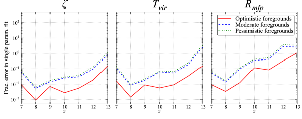
Figure 14.— Fractional $1\sigma$ errors ($1\sigma$ errors divided by fiducial values) as a function of redshift, with measurements at each redshift fit independently. The errors on each parameter assume (unrealistically) that all other parameters are already known in the fit. Solid red curves give optimistic foreground model predictions; dashed blue curves give moderate foreground model predictions; dot-dashed green curves give pessimistic foreground model predictions. In all models, and for all three parameters, the best errors are obtained at $z=8$. At $z=7$, the power spectrum has too small of an amplitude to yield good signal-to-noise, and at higher redshifts thermal noise poses a serious problem.

Of course, what is not captured by Figure 14 is the reality that one must fit for all parameters simultaneously (since none of our three parameters are currently strongly constrained by other observational probes). In general, our ability to constrain model parameters is determined not just by the amplitudes of the power spectrum derivatives and our instrument’s sensitivity, but also by parameter degeneracies. As an example, notice that at $z=7$, all the power spectrum derivatives shown in Figure 12 have essentially identical shapes up to a sign. This means that shifts in one parameter can be (almost) perfectly nullified by a shift in a different parameter; the parameters are degenerate. These degeneracies are inherent to the theoretical model, since they are clearly visible even in Figure 12, where the power spectrum derivatives are shown without the instrumental weighting. With this in mind, we see that even though Figure 14 predicts that observing the power spectrum at $z=7$ alone would give reasonable errors if there were somehow no degeneracies (making a single parameter fit the same as a simultaneous fit), such a measurement would be unlikely to yield any useful parameter constraints in practice. To only a slightly lesser extent, the same is true for $z=8$, where the degeneracy between $R_{\textrm{mfp}}$ and the other parameters is broken slightly, but $T_{\textrm{vir}}$ and $\zeta$ remain almost perfectly degenerate.

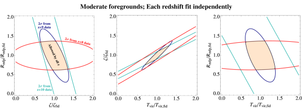
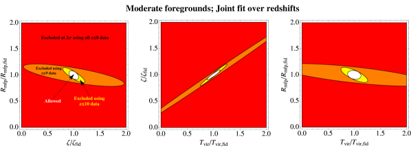
Figure 15.— Pairwise parameter constraints for the moderate foreground model, shown as $2\sigma$ exclusion regions. For each pair of parameters, the third parameter has been marginalized over. The top row shows $2\sigma$ constraints from each redshift when fit independently; the light orange regions are not ruled out by data from any redshifts. The bottom row shows the constraints from a joint fit over multiple redshifts. Each color represents a portion of parameter space that can be excluded by including data up to a certain redshift. The white “allowed” region represents the final constraints from including all measured redshifts. In both cases, a $z=7$ measurement alone does not provide any non-trivial constraints, but helps with degeneracy-breaking in the joint redshift fits (bottom row). As one moves to higher and higher redshifts, power spectrum measurements probe different astrophysical processes, resulting in a shift in the principal directions of the exclusion regions. Including higher redshifts tightens parameter constraints, but no longer helps beyond $z=10$ due to increasing thermal noise.

The situation becomes even worse when one realizes that measurements at low and high $k$ are difficult due to foregrounds and thermal noise, respectively. Many of the distinguishing features between the curves in Figure 12 were located at the extremes of the $k$ axis, and from Figure 13, we see that such features are obliterated by an instrumental sensitivity weighting (particularly for the pessimistic/moderate foregrounds). This increases the level of degeneracy. As an aside, note that with the lowest and highest $k$ values cut out, the bulk of the information originates from $k\sim 0.05~{}h\textrm{Mpc}^{-1}$ to $\sim 1~{}h\textrm{Mpc}^{-1}$ for the optimistic model and $k\sim 0.2~{}h\textrm{Mpc}^{-1}$ to $\sim 1~{}h\textrm{Mpc}^{-1}$ for the pessimistic and moderate models. (Recall again that since elements of the Fisher matrix are obtained by taking pairwise products of the rows of Figure 13 and summing over $k$ and $z$, the square of each weighted power spectrum derivative curve provides a rough estimate for where information comes from.) Matching these ranges to the fiducial power spectra in Figure 3 confirms the qualitative discussion presented in Section 3.4, where we saw that slope of the power spectrum from $k\sim 0.1~{}h\textrm{Mpc}^{-1}$ to $\sim 1~{}h\textrm{Mpc}^{-1}$ is potentially a useful source of information regardless of foreground scenario, but that the “knee” feature at $k\lesssim 0.1~{}h\textrm{Mpc}^{-1}$ will likely only be accessible with optimistic foregrounds. This is somewhat unfortunate, for a comparison of Figures 12 and 13 reveals that measurements at low and high $k$ would potentially be powerful breakers of degeneracy, were they observationally feasible.

3.6.2 Breaking degeneracies with multi-redshift observations

Absent a situation where the lowest and highest $k$ values can be probed, the only way to break the serious degeneracies in the high signal-to-noise measurements at $z=7$ and $z=8$ is to include higher redshifts, even though thermal noise and foreground limitations dictate that such measurements will be less sensitive. Higher redshift measurements break degeneracies in two ways. First, one can see that at higher redshifts, the power spectrum derivatives have shapes that are both more complicated and less similar, thanks to non-trivial astrophysics during early to mid-reionization. Second, a joint fit over multiple redshifts can alleviate degeneracies even if the parameters are perfectly degenerate with each other at every redshift when fit on a per-redshift basis. Consider, for example, the weighted power spectrum derivatives for the moderate foreground model in Figure 13. For both $z=7$ and $z=8$, the derivatives for all three parameters are identical in shape; at both redshifts, any shift in the best-fit value of a parameter can be compensated for by an appropriate shift in the other parameters without compromising the goodness-of-fit. At $z=8$, for instance, a given fractional increase in $\zeta$ can be compensated for by a slightly larger decrease in $R_{\textrm{mfp}}$, since $w_{\textrm{Rmfp}}$ has a slightly larger amplitude than $w_{\zeta}$. However, this only works if the redshifts are treated independently. If the data from $z=7$ and $z=8$ are jointly fit, the aforementioned parameter shifts would result in a worse overall fit, because $w_{\textrm{Rmfp}}$ and $w_{\zeta}$ have roughly equal amplitudes at $z=7$, demanding fractionally equal shifts. In other words, we see that because the ratios of different weighted parameter derivatives are redshift-dependent quantities, joint-redshift fits can break degeneracies even when the parameters would be degenerate if different redshifts were treated independently. It is therefore crucial to make observations at a wide variety of redshifts, and not just at the lowest ones, where the measurements are easiest.

To see how degeneracies are broken by using information from multiple redshifts, imagine a thought experiment where one began with measurements at the lowest (least noisy) redshifts, and gradually added higher redshift information, one redshift at a time. Figures 15 and 16 show the results for the moderate and optimistic foreground scenarios respectively. (Here we omit the equivalent figure for the pessimistic model completely, because the results are again qualitatively similar to those for the moderate model.) In each figure are $2\sigma$ constraints for pairs of parameters, having marginalized over the third parameter by assuming that the likelihood function is Gaussian (so that the covariance of the measured parameters is given by the inverse of the Fisher matrix). One sees that as higher and higher redshifts are included, the principal directions of the exclusion ellipses change, reflecting the first degeneracy-breaking effect highlighted above, namely, the inclusion of different, more-complex and less-degenerate astrophysics at higher redshifts. To see the second degeneracy-breaking effect, where per-redshift degeneracies are broken by joint redshift fits, we include in both figures the constraints that arise after combining results from redshift-by-redshift fits (shown as contours for each redshift), as well as the constraints from fitting multiple redshifts simultaneously (shown as cumulative exclusion regions).

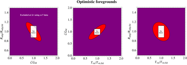
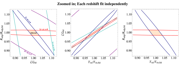
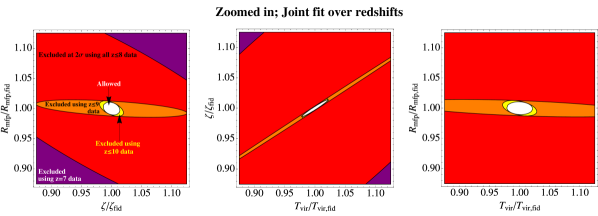
Figure 16.— Similar to Figure 15, but for the optimistic foreground model. The top row shows the exclusion region from using $z=7$ data alone. The middle and bottom rows show zoomed-in parameter space plots for the redshift-by-redshift and simultaneous fits respectively. (Since $z=7$ is the lowest redshift in our model, the top panel is the same for both types of fit). The constraints in this optimistic foreground scenario are seen to be better than those predicted for the moderate foreground model by about a factor of four.

For the moderate foreground scenario, we find that non-trivial constraints cannot be placed using $z=7$ data alone, hence the omission of a $z\leq 7$ exclusion region from Figure 15. However, we note that the constraints using $z\leq 8$ data (red contours/exclusion regions) are substantially tighter in the bottom panel than in the top panel of the figure. This means that the $z=7$ power spectrum can break degeneracies in a joint fit, even if the constraints from it alone are too degenerate to be useful. A similar situation is seen to be true for a $z=10$ measurement, which is limited not just by degeneracy, but also by the higher thermal noise at lower frequencies. Except for the $\zeta$-$T_{\textrm{vir}}$ parameter space, adding $z=10$ information in an independent fashion does not further tighten the constraints beyond those provided by $z\leq 9$. But again, when a joint fit (bottom panel of Figure 15) is performed, this information is useful even though it was noisy and degenerate on its own. We caution, however, that this trend does not persist beyond $z=10$, in that $z\geq 11$ measurements are so thermal-noise dominated that their inclusion has no effect on the final constraints. Indeed, the “allowed” regions in both Figures 15 and 16 include all redshifts, but are visually indistinguishable from ones calculated without $z\geq 11$ information.

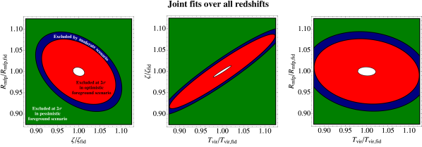
Figure 17.— A comparison between the $2\sigma$ exclusion regions for pessimistic (green), moderate (blue), and optimistic (red) foregrounds, assuming that power spectra at all measured redshifts are fit simultaneously. Going from the pessimistic foreground model to the moderate model gives only marginal improvement; going from the moderate to the optimistic model reduces errors from the $5\%$ level to the $1\%$ level.

Comparing the predictions for the moderate foreground model to those of the optimistic foreground model (Figure 16), several differences are immediately apparent. Whereas the $z=7$ power spectrum alone could not place non-trivial parameter constraints in the moderate scenario, in the optimistic scenario it has considerable discriminating power, similar to what can be achieved by jointly fitting all $z\leq 9$ data in the moderate model. This improvement in the effectiveness of the $z=7$ measurement is due to an increased ability to access low and high $k$ modes, which breaks degeneracies. With low and high $k$ modes measurable, each redshift alone is already reasonably non-degenerate, and the main benefit (as far as degeneracy-breaking is concerned) in going to higher $z$ is the opportunity to access new astrophysics with a slightly different set of degeneracies, rather than the opportunity to perform joint fits. Indeed, we see from the middle and bottom panels of Figure 16 that there are only minimal differences between the joint fit and the independent fits. In contrast, with the moderate model in Figure 15 we saw about a factor of four improvement in going from the latter to the former.

Foreground Model	$\Delta T_{\textrm{vir}}/T_{\textrm{vir,fid}}$	$\Delta\zeta$/$\zeta_{\textrm{fid}}$	$\Delta R_{\textrm{mfp}}/R_{\textrm{mfp,fid}}$
Moderate	$0.062$	$0.044$	$0.039$
Pessimistic	$0.071$	$0.051$	$0.047$
Optimistic	$0.011$	$0.0069$	$0.0052$

Table 2Reionization Parameter Errors ($1\sigma$) for HERA

Figure 17 compares the ultimate performance of HERA for the three foreground scenarios, using all measured redshifts in a joint fit. (Note that our earlier emphasis on the differences between joint fits and independent fits was for pedagogical reasons only, since in practice there is no reason not to get the most out of one’s data by performing a joint fit.) We see that even with the most pessimistic foreground model, our three parameters can be constrained to the $5\%$ level. The ability to combine partially-coherent baselines in the moderate model results only in a modest improvement, but being able to work within the wedge in the optimistic case can suppress errors to the $\sim 1\%$ level. The final results are given in Table 2.

In closing, we see that a next-generation like HERA should be capable of delivering excellent constraints on astrophysical parameters during the EoR. These constraints will be particularly valuable, given that none of the parameters can be easily probed by other observations. However, a few qualifications are in order. First, the Fisher matrix analysis performed here provides an accurate forecast of the errors only if the true parameter values are somewhat close to our fiducial ones. As an extreme example of how this could break down, suppose $T_{\textrm{vir}}$ were actually $1000\,\textrm{K}$, as illustrated in the middle row of Figure 4. The result would be a high-redshift reionization scenario, one that would be difficult to probe to the precision demonstrated in this section, due to high thermal noise. Secondly, one’s ability to extract interesting astrophysical quantities from a measurement of the power spectrum is only as good as one’s ability to model the power spectrum. In this section, we assumed that 21cmFAST is the “true” model of reionization. At the few-percent-level uncertainties given in Table 2, the measurement errors are better than or comparable to the scatter seen between different theoretical simulations (Zahn et al., 2011). Thus, there will likely need to be much feedback between theory and observation to make sense of a power spectrum measurement with HERA-level precision. Alternatively, given the small error bars seen here with a three-parameter model, it is likely that additional parameters can be added to one’s power spectrum fits without sacrificing the ability to place constraints that are theoretically interesting. We leave the possibility of including additional parameters (many of which have smaller, subtler effects on the $21\,\textrm{cm}$ power spectrum than the parameters examined here) for future work.

4. Conclusions

In order to explore the potential range of constraints that will come from the proposed next generation of 21 cm experiments (e.g. HERA and SKA), we used simple models for instruments, foregrounds, and reionization histories to encompass a broad range of possible scenarios. For an instrument model, we used the $\sim 0.1~{}\rm{km}^{2}$ HERA concept array, and calculated power spectrum sensitivities using the method of Pober et al. (2013b). To cover uncertainties in the foregrounds, we used three principal models. Both our pessimistic and moderate model assumes foregrounds occupy the wedge-like region in $k$-space observed by Pober et al. (2013a), extending $0.1~{}h{\rm Mpc}^{-1}$ past the analytic horizon limit. Thus, both cases are amenable to a strategy of foreground avoidance. What makes our pessimistic model pessimistic is the decision to combine partially redundant baselines in an incoherent fashion, allowing one to completely sidestep the systematics highlighted by Hazelton et al. (2013). In the moderate model, these baselines are allowed to be combined coherently. Finally, in our optimistic model, the size of the wedge is reduced to a region defined by the FWHM of the primary beam. Given the small field of view of the dishes used in the HERA concept array, this model is effectively equivalent to one in which foreground removal techniques prove successful. Lastly, to cover the uncertainties in reionization history, we use 21cmFAST to generate power spectra for a wide range of uncertain parameters: the ionizing efficiency $\zeta$, the minimum virial temperature of halos producing ionizing photos, $T_{\rm vir}$, and the mean free path of ionizing photons through the IGM $R_{\rm mfp}$.

Looking at predicted power spectrum measurements for these various scenarios yields the following conclusions:

• Even with no development of analysis techniques beyond those used in Parsons et al. (2013), an experiment with $\sim 0.1~{}\rm{km}^{2}$ of collecting area can yield very high significance $\gtrsim 30\sigma$ detections of nearly any reionization power spectrum (cf. Figure 7).

• Developing techniques that allow for the coherent addition of partially redundant baselines can result in a small increase of additional power spectrum sensitivity. In this work, we find our moderate foreground removal model to increase sensitivities by $\sim 20\%$ over our most pessimistic scenario. Generally, we find that coherent combination of partially redundant baselines reduces thermal noise errors by $\sim 40\%$, so addressing this issue will be somewhat more important for smaller arrays that have not yet reached the sample variance dominated regime.

• With the sensitivities achievable with our moderate foreground model, the next generation of arrays will yield high significance detections of the EoR power spectra, and provide detailed characterization of the power spectrum shape over an order-of-magnitude in $k$ ($k\sim 0.1\mbox{--}1.0h{\rm Mpc}^{-1}$). These sensitivity levels may even allow for direct imaging of the EoR on these scales.

• If successful, foreground removal algorithms can dramatically boost the sensitivity of 21 cm measurements. They are also the only way to open up the largest scales of the power spectrum, which can lead to new physical insight through observations of the generic “knee” feature.

• Although it will represent a major breakthrough for the 21 cm cosmology community, a low to moderate ($\sim 5\mbox{--}10\sigma$) detection of the EoR power spectrum may not be able to conclusively identify the redshift of 50% ionization. One might expect otherwise, since the peak brightness of the power spectrum occurs near this ionization fraction. However, accounting for the steep rise in $T_{\rm sys}$ at low frequencies, shows that the rise-and-fall of the power spectrum versus redshift may not be conclusively measurable without a higher significance measurement, such as those possible with the HERA design.

• Going beyond power spectrum measurements to astrophysical parameter constraints, lower redshifts observations are particularly prone to parameter degeneracies. These can be partially broken by foreground removal from within the wedge region (allowing access to the lowest $k$ modes). Alternatively, degeneracies can be broken by performing parameter fits over multiple redshifts simultaneously (which is equivalent to making use of information about the power spectrum’s evolution). Higher redshifts ($z\geq 11$) are typically limited not by intrinsic degeneracies, but by high thermal noise (at least for a HERA-like array), and add relatively little to constraints on reionization.

• Assuming a fiducial 21cmFAST reionization model, a HERA-like array will be capable of constraining reionization parameters to $\sim 1\%$ uncertainty if foreground removal within the wedge proves possible, and to $\sim 5\%$ otherwise. The current generation of interferometers will struggle to provide precise constraints on reionization models; the sensitivity of a HERA-like array is necessary for this kind of science (for a quantitative comparison, see the appendix).

From this analysis, it is clear that for 21 cm studies to deliver the first conclusive scientific constraints on the Epoch of Reionization, arrays much larger than those currently operational must be constructed. Advancements in analysis techniques to keep the EoR window free from contamination can contribute additional sensitivity, but the most dramatic gains on the analysis front will come from techniques that remove foreground emission and allow retrieval of modes from inside the wedge. This is not meant to disparage the wide range of foreground removal techniques already in the literature; rather, the impetus is on adapting these techniques for application to real data from the current and next generation of 21 cm experiments. The vast range of EoR science achievable under our optimistic, moderate, and even pessimistic foreground removal scenarios provides ample motivation for continuing these efforts.

Appendix A Power Spectrum Sensitivities of Other 21 cm Experiments

In this appendix, we compare the power spectrum sensitivities and EoR parameter constraints of several 21 cm experiments. In particular, we consider the current generation experiments of PAPER (Parsons et al., 2010), the MWA (Tingay et al., 2013), and LOFAR (van Haarlem et al., 2013), as well as a concept array for Phase 1 of the SKA based on the SKA System Baseline Design document (SKA-TEL-SKO-DD-001). The instrument designs are summarized in Table LABEL:tab:instruments, and the principal results are presented in Tables 3 and 4, which show the significance of the power spectrum measurements and constraints on EoR astrophysical parameters, respectively. Both calculations assume the fiducial EoR history shown in Figure 3. The significances in Table 3 assume only an 8 MHz band centered on the 50% ionization redshift of $z=9.5$. The astrophysical constraints, however, assume information is collected over a wider band from $z=7\mbox{--}13$; for instruments with smaller instantaneous bandwidths, the observing times will need to be adjusted accordingly.

[ caption=Properties of Other 21 cm Experiments, label=tab:instruments, pos=ht, mincapwidth=]c—p.66inp.66inp.7inp3.3in [a]Assumes each HBA sub-station is correlated independently. Instrument Number of Elements Element Size $(\rm{m}^{2})$ Collecting Area $(\rm{m}^{2})$ Configuration
PAPER 132 9 1188 $11\times 12$ sparse grid
MWA 128 28 3584 Dense 100 m core with $r^{-2}$ distribution beyond
LOFAR NL Core 48[a] 745 35,762 Dense 2 km core
HERA 547 154 84,238 Filled 200 m hexagon
SKA1 Low Core 866 962 833,190 Filled 270 m core with Gaussian distribution beyond

Instrument	Pessimistic	Moderate	Optimistic
PAPER	1.17	2.02	4.82
MWA	0.60	2.46	6.40
LOFAR NL Core	1.35	2.76	17.37
HERA	32.09	38.20	133.15
SKA1 Low Core	10.01	35.95	218.27

Table 3Power spectrum measurement signifiance (number of $\sigma$s) of other 21 cm experiments for each of the three foreground removal models.

	Pessimistic			Moderate			Optimistic
Instrument	$\frac{\Delta T_{\rm vir}}{T_{\rm vir,fid}}$	$\frac{\Delta\zeta}{\zeta_{\rm fid}}$	$\frac{\Delta R_{\rm mfp}}{R_{\rm mfp,fid}}$	$\frac{\Delta T_{\rm vir}}{T_{\rm vir,fid}}$	$\frac{\Delta\zeta}{\zeta_{\rm fid}}$	$\frac{\Delta R_{\rm mfp}}{R_{\rm mfp,fid}}$	$\frac{\Delta T_{\rm vir}}{T_{\rm vir,fid}}$	$\frac{\Delta\zeta}{\zeta_{\rm fid}}$	$\frac{\Delta R_{\rm mfp}}{R_{\rm mfp,fid}}$
PAPER	1.444	1.168	1.507	1.260	1.013	1.294	0.272	0.179	0.140
MWA	4.419	3.479	4.555	0.757	0.568	0.731	0.231	0.152	0.119
LOFAR	1.538	1.251	1.515	0.719	0.565	0.675	0.069	0.046	0.039
HERA	0.072	0.051	0.047	0.062	0.044	0.039	0.011	0.007	0.005
SKA1	0.235	0.169	0.179	0.076	0.054	0.044	0.009	0.006	0.004

Table 4Fractional errors on the reionization parameters achieveable with each instrument under the three foreground removal models, assuming all redshifts are analyzed jointly.

In order to compute the constraints achievable with other experiments, we apply the sensitivity calculation described in §2.1.1 to each of the five instruments under study. We note that this sensitivity calculation assumes a drift-scanning observing mode, with the limit of coherent sampling set by the size of the element primary beam. The MWA, LOFAR, and likely the SKA all have the capability of conducting a tracked scan to increase the coherent integration on a single patch of sky. Similarly, tracking can be used to move to declinations away from zenith if sample variance becomes the dominant source of error. A full study of the benefits of tracking versus draft scanning for power spectrum measurements is beyond the scope of this present work; rather, we assume all instruments operate in a drift-scanning mode for the clearest comparison with the fiducial results calculated for the HERA experiment. We therefore also assume that each telescope observes for the fiducial 6 hours per day for 180 days (1080 hours). Finally, we also assume that each array has a receiver temperature of 100 K. We discuss the important features of each instrument and the resultant constraints in turn; see the main text for a discussion of the HERA experiment.

1. PAPER: Our fiducial PAPER instrument is an $11\times 12$ grid of PAPER dipoles modelled after the maximum redundancy arrays presented in Parsons et al. (2012a). In this configuration, the $3\times 3~{}\rm{m}$ dipoles are spaced in 12 north-south columns separated by 16 m; within a column, the dipoles are spaced 4 m apart. In both our pessimistic and moderate scenarios, PAPER yields a non-detection of the fiducial 21 cm power spectrum. In the optimistic scenario, the array could yield a significant detection; however, the poor PSF of the maximum redundancy array is expected to present challenges to any foreground-removal strategy that would allow recovery from information inside the wedge (Parsons et al., 2013). Therefore, achieving the results of the optimistic scenario will be especially difficult for the PAPER experiment.

2. MWA: Our model MWA array uses the 128 antenna positions presented in Tingay et al. (2013). Despite having nearly three times the collecting area of the PAPER array, we find the MWA yields a less significant detection in the pessimistic scenario. Poor sensitivity when partially redundant samples are combined incoherently is to be expected for the MWA. The pseudo-random configuration of the array produces essentially no instantaneously redundant samples, and so all redundancy comes from partial coherence. Therefore, one might expect the MWA to under-perform compared to the highly redundant PAPER array in this scenario. In the moderate and optimistic scenarios where partial redundancy yields sensitivity boosts the MWA outperforms the PAPER array.

3. LOFAR: To model the LOFAR array, we use the antenna positions presented in van Haarlem et al. (2013). For the purposes of EoR power spectrum studies, we focus on the Netherlands core of the instrument, since baselines much longer than a few km contribute very little sensitivity. We also assume that LOFAR is operated in a mode where each sub-station of the HBA is correlated separately to increase the number of short baselines. However, the resultant sensitivities still show that LOFAR suffers from a lack of short baselines. Despite having a collecting area $\gtrsim 10$ times larger than PAPER and the MWA, LOFAR still yields a non-detection of the EoR power spectrum in the pessimistic and moderate foreground removal scenarios. Only in the optimistic scenario where longer baselines contribute to the power spectrum measurements does LOFAR’s collecting area result in a high-significance measurement. Preliminary results from the LOFAR experiment show significant progress in subtracting foregrounds to access modes inside the wedge (Chapman et al., 2012; Yatawatta et al., 2013).

4. SKA1-Low: We model our SKA-Low Phase 1 instrument after the design parameters set out in the SKA System Baseline Design document, although the final design of the SKA is still subject to change. This document specifies that the array will consist of 911 35 m stations, with 866 stations in a core with a Gaussian distribution versus radius. This distribution is normalized to have 650 stations within a radius of 1 km. This density in fact yields a completely filled aperture out to $\sim 300~{}\rm{m}$, which we model as a close packed hexagon. This core gives the design some degree of instantaneous redundancy, a configuration that is still being explored for the final design of the instrument. We do not consider the 45 outriggers in our power spectrum sensitivity. Much like the case with PAPER and the MWA, the lower instantaneous redundancy of the SKA concept array results in a poorer performance than the highly redundant HERA array in the pessimistic scenario. However, in the moderate and optimistic scenarios this SKA concept design yields high sensitivity measurements, although not as high as might be expected from collecting area alone. This fact is once again due to the relatively small number of short spacings compared to the HERA array, resulting in similar performances for the two configurations in the moderate scenario. As with LOFAR, the SKA design shines in the optimistic scenario, producing a very high SNR measurement.

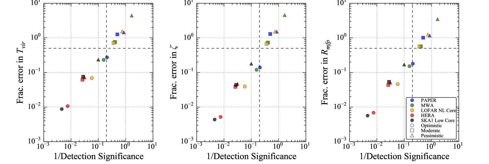
Figure 18.— Fractional errors in astrophysical parameters shown as a function of $(\textrm{detection significance})^{-1}$. Different instruments are shown in different colors (PAPER in blue; MWA in green; LOFAR in yellow; HERA in red; SKA in black), and different foreground scenarios are shown using different shapes (optimistic as circles; moderate as squares; pessimistic as triangles). The vertical dashed line delineates a $5\sigma$ detection of the power spectrum, while the horizontal dashed line delineates a parameter error of $50\%$. The tight correlations shown here suggest that the significance of a power spectrum detection can be used as a proxy for an instrument’s ability to constrain astrophysical parameters.

In all cases, we find that the fractional errors on the reionization parameters (Table 4) scale very closely with the overall significance of the power spectrum measurement (Table 3). This is shown in Figure 18, where we plot the fractional errors on the reionization parameters against the reciprocal of the power spectrum detection significance. These two quantities are seen to be directly proportional to an excellent approximation, regardless of foreground scenario. Therefore, while the power spectrum sensitivity of an array can be a strong function of an instrument’s configuration, the resultant astrophysical constraints are fairly generalizable once the instrument sensitivity is known. This is strongly suggestive that the results in the main body of the paper can be easily extended to other instruments. Also noteworthy is the fact that current-generation instruments encroach on the lower-left regions (high detection significance; small parameter errors) of the plots in Figure 18 only for the optimistic foreground model. In contrast, the next-generation instruments (HERA and SKA) are clearly capable of delivering excellent scientific results even in the most pessimistic foreground scenario.

References

- Abel et al. (2002) Abel, T., Bryan, G. L., & Norman, M. L. 2002, Science, 295, 93
- Barkana & Loeb (2007) Barkana, R., & Loeb, A. 2007, Reports on Progress in Physics, 70, 627
- Beardsley et al. (2013) Beardsley, A. P., et al. 2013, MNRAS, 429, L5
- Bernardi et al. (2013) Bernardi, G., et al. 2013, ApJ, 771, 105
- Bittner & Loeb (2011) Bittner, J. M., & Loeb, A. 2011, Journal of Cosmology and Astroparticle Physics, 4, 38
- Bowman et al. (2006) Bowman, J. D., Morales, M. F., & Hewitt, J. N. 2006, ApJ, 638, 20
- Bowman et al. (2007) —. 2007, ApJ, 661, 1
- Bowman et al. (2009) —. 2009, ApJ, 695, 183
- Bowman et al. (2013) Bowman, J. D., et al. 2013, Publications of the Astronomical Society of Australia, 30, 31
- Bromm et al. (2002) Bromm, V., Coppi, P. S., & Larson, R. B. 2002, ApJ, 564, 23
- Chapman et al. (2012) Chapman, E., et al. 2012, MNRAS, 423, 2518
- Chapman et al. (2013) —. 2013, MNRAS, 429, 165
- Christian & Loeb (2013) Christian, P., & Loeb, A. 2013, Journal of Cosmology and Astroparticle Physics, 9, 14
- Datta et al. (2010) Datta, A., Bowman, J. D., & Carilli, C. L. 2010, ApJ, 724, 526
- Datta et al. (2012) Datta, K. K., Mellema, G., Mao, Y., Iliev, I. T., Shapiro, P. R., & Ahn, K. 2012, MNRAS, 424, 1877
- de Oliveira-Costa et al. (2008) de Oliveira-Costa, A., Tegmark, M., Gaensler, B. M., Jonas, J., Landecker, T. L., & Reich, P. 2008, MNRAS, 388, 247
- Dillon et al. (2013a) Dillon, J. S., Liu, A., & Tegmark, M. 2013a, Phys. Rev. D, 87, 043005
- Dillon et al. (2013b) Dillon, J. S., et al. 2013b, ArXiv e-prints
- Fan et al. (2006) Fan, X., et al. 2006, AJ, 131, 1203
- Furlanetto et al. (2006a) Furlanetto, S. R., McQuinn, M., & Hernquist, L. 2006a, MNRAS, 365, 115
- Furlanetto et al. (2006b) Furlanetto, S. R., Oh, S. P., & Briggs, F. H. 2006b, Phys. Rep., 433, 181
- Furlanetto et al. (2004) Furlanetto, S. R., Zaldarriaga, M., & Hernquist, L. 2004, ApJ, 613, 16
- Haiman et al. (1996) Haiman, Z., Thoul, A. A., & Loeb, A. 1996, ApJ, 464, 523
- Hazelton et al. (2013) Hazelton, B. J., Morales, M. F., & Sullivan, I. S. 2013, ApJ, 770, 156
- Hinshaw et al. (2012) Hinshaw, G., et al. 2012, ArXiv e-prints
- Iliev et al. (2012) Iliev, I. T., Mellema, G., Shapiro, P. R., Pen, U.-L., Mao, Y., Koda, J., & Ahn, K. 2012, MNRAS, 423, 2222
- La Plante et al. (2013) La Plante, P., Battaglia, N., Natarajan, A., Peterson, J. B., Trac, H., Cen, R., & Loeb, A. 2013, ArXiv e-prints
- Lidz et al. (2008) Lidz, A., Zahn, O., McQuinn, M., Zaldarriaga, M., & Hernquist, L. 2008, ApJ, 680, 962
- Liu & Tegmark (2011) Liu, A., & Tegmark, M. 2011, Phys. Rev. D, 83, 103006
- Liu et al. (2009) Liu, A., Tegmark, M., Bowman, J., Hewitt, J., & Zaldarriaga, M. 2009, MNRAS, 398, 401
- Loeb & Furlanetto (2013) Loeb, A., & Furlanetto, S. R. 2013, The First Galaxies In The Universe (Princeton University Press)
- McQuinn et al. (2006) McQuinn, M., Zahn, O., Zaldarriaga, M., Hernquist, L., & Furlanetto, S. R. 2006, ApJ, 653, 815
- Mesinger & Dijkstra (2008) Mesinger, A., & Dijkstra, M. 2008, MNRAS, 390, 1071
- Mesinger et al. (2013) Mesinger, A., Ewall-Wice, A., & Hewitt, J. 2013, ArXiv e-prints
- Mesinger & Furlanetto (2007) Mesinger, A., & Furlanetto, S. 2007, ApJ, 669, 663
- Mesinger et al. (2011) Mesinger, A., Furlanetto, S., & Cen, R. 2011, MNRAS, 411, 955
- Mesinger et al. (2012) Mesinger, A., McQuinn, M., & Spergel, D. N. 2012, MNRAS, 422, 1403
- Moore et al. (2013) Moore, D. F., Aguirre, J. E., Parsons, A. R., Jacobs, D. C., & Pober, J. C. 2013, ArXiv e-prints
- Morales (2005) Morales, M. F. 2005, ApJ, 619, 678
- Morales et al. (2006) Morales, M. F., Bowman, J. D., & Hewitt, J. N. 2006, ApJ, 648, 767
- Morales et al. (2012) Morales, M. F., Hazelton, B., Sullivan, I., & Beardsley, A. 2012, ApJ, 752, 137
- Morales & Wyithe (2010) Morales, M. F., & Wyithe, J. S. B. 2010, ARA&A, 48, 127
- Okamoto et al. (2008) Okamoto, T., Gao, L., & Theuns, T. 2008, MNRAS, 390, 920
- Parsons et al. (2012a) Parsons, A., Pober, J., McQuinn, M., Jacobs, D., & Aguirre, J. 2012a, ApJ, 753, 81
- Parsons et al. (2012b) Parsons, A. R., Pober, J. C., Aguirre, J. E., Carilli, C. L., Jacobs, D. C., & Moore, D. F. 2012b, ApJ, 756, 165
- Parsons et al. (2010) Parsons, A. R., et al. 2010, AJ, 139, 1468
- Parsons et al. (2013) —. 2013, ArXiv e-prints
- Pober et al. (2013a) Pober, J. C., et al. 2013a, ApJ, 768, L36
- Pober et al. (2013b) —. 2013b, AJ, 145, 65
- Pritchard & Loeb (2012) Pritchard, J. R., & Loeb, A. 2012, Reports on Progress in Physics, 75, 086901
- Songaila & Cowie (2010) Songaila, A., & Cowie, L. L. 2010, ApJ, 721, 1448
- Tegmark et al. (1997) Tegmark, M., Taylor, A. N., & Heavens, A. F. 1997, ApJ, 480, 22
- Thompson et al. (2007) Thompson, A. R., Moran, J. M., & Swenson, G. W. 2007, Interferometry and Synthesis in Radio Astronomy, John Wiley & Sons, 2007.
- Thyagarajan et al. (2013) Thyagarajan, N., et al. 2013, ApJ, 776, 6
- Tingay et al. (2013) Tingay, S. J., et al. 2013, Publications of the Astronomical Society of Australia, 30, 7
- Trac & Cen (2007) Trac, H., & Cen, R. 2007, ApJ, 671, 1
- Trott et al. (2012) Trott, C. M., Wayth, R. B., & Tingay, S. J. 2012, ApJ, 757, 101
- van Haarlem et al. (2013) van Haarlem, M. P., et al. 2013, A&A, 556, A2
- Vedantham et al. (2012) Vedantham, H., Udaya Shankar, N., & Subrahmanyan, R. 2012, ApJ, 745, 176
- Yatawatta et al. (2013) Yatawatta, S., et al. 2013, ArXiv e-prints
- Zahn et al. (2011) Zahn, O., Mesinger, A., McQuinn, M., Trac, H., Cen, R., & Hernquist, L. E. 2011, MNRAS, 414, 727
- Zaldarriaga et al. (2004) Zaldarriaga, M., Furlanetto, S. R., & Hernquist, L. 2004, ApJ, 608, 622