Magnetic field structure and torque in accretion discs around millisecond pulsars

Abstract

Millisecond pulsars are rather weakly-magnetized neutron stars which are thought to have been spun up by disc accretion, with magnetic linkage between the star and the disc playing a key role. Their spin history depends sensitively on details of the magnetic field structure, but idealized models from the 1980s and 1990s are still commonly used for calculating the magnetic field components. This paper is the third in a series presenting results from a step-by-step analysis which we are making of the problem, starting with very simple models and then progressively including additional features one at a time, with the aim of gaining new insights into the mechanisms involved. In our first two papers, the magnetic field structure in the disc was calculated for a standard Shakura/Sunyaev model, by solving the magnetic induction equation numerically in the stationary limit within the kinematic approximation; here we consider a more general velocity field in the disc, including backflow. We find that the profiles of the poloidal and toroidal components of the magnetic field are fairly similar in the two cases but that they can be very different from those in the models mentioned above, giving important consequences for the torque exerted on the central object. In particular we find that, contrary to what is usually thought, some regions of the disc outward of the co-rotation point (rotating more slowly than the neutron star) may nevertheless contribute to spinning up the neutron star on account of the detailed structure of the magnetic field in those parts of disc.

1 Introduction

Accretion discs around magnetized neutron stars can greatly influence the stellar magnetic field, and magnetic field deformations can in turn have an effect on the angular momentum exchange between the disc and the central object. Here we investigate these deformations and their effect on the neutron star spin. We focus mostly on the progenitors of millisecond pulsars, which are commonly believed to be descendants of normal neutron stars that have been spun up and recycled back as radio pulsars by acquiring angular momentum from their companion via an accretion disc during the low-mass X-ray binary phase (Alpar et al., 1982; Radhakrishnan & Srinivasan, 1982).

The importance of magnetic fields in accretion discs around neutron stars was recognized already in the early paper by Pringle & Rees (1972). It was already clear then that the most relevant character in the play is the profile of the toroidal component of the magnetic field, $B_{\phi}$. However, it was only in Ghosh & Lamb (1979a) that a detailed model was developed. They pointed out that turbulent motion, reconnection and the Kelvin–Helmholtz instability allow the stellar field to penetrate the disc and hence to be affected by its velocity field. By assuming a dipole profile for the poloidal component of the magnetic field, they calculated a corresponding profile for $B_{\phi}$.

One of the main consequences of having a non-zero Lorentz force inside the disc is the creation of a magnetic torque, which can drastically influence the spin history of the central object and also change the shape of the disc. Ghosh & Lamb (1979b) used the solution obtained in Ghosh & Lamb (1979a) to compute the torque exerted on the neutron star by a Keplerian disc. However in Wang (1987) it was shown that the solution obtained by Ghosh & Lamb (1979a) violated the induction equation and a consistent analytic profile for the toroidal field was instead calculated, as a stationary solution of the induction equation in axisymmetry. In that model the poloidal component of the magnetic field was assumed to be a pure dipole; the disc was assumed to be Keplerian, to be in corotation with the neutron star at the upper and lower surfaces and not to have any motion along the poloidal direction; also, all horizontal derivatives were neglected with respect to vertical derivatives. At almost the same time, Campbell (1987) developed a similar one-dimensional model where, in addition, a non-Keplerian profile for the disc was considered and where the horizontal terms in the induction equations were also included. Both authors agreed in writing the toroidal component of the magnetic field in the following form, in cylindrical coordinates $(\varpi,\phi,z)$:

$$B_{\phi}=\gamma_{\rm a}\,(\Omega_{\rm disc}-\Omega_{\rm s})\,B_{z}\,\tau_{\rm d}\,\,{\rm,}$$ (1)

where $\gamma_{\rm a}$ is the amplification factor, $\Omega_{\rm disc}$ and $\Omega_{\rm s}$ are the disc and stellar angular velocities, respectively, and $\tau_{\rm d}$ is the dissipation time–scale. For a dipole $B_{z}$, equation (1) implies $B_{\phi}\propto\,\Delta\Omega/\varpi^{3}$, where $\Delta\Omega\equiv\Omega_{\rm disc}-\Omega_{\rm s}$. In these models, the amplification factor $\gamma_{\rm a}$ was taken to be a constant not much greater than unity (it depends on the steepness of the transition in $\Omega$, from disc motion in the equatorial plane to corotation at the disc surface). The precise profile of $\tau_{\rm d}$ depends on what is the dominant mechanism for dissipating the magnetic field. Wang (1995) considered three different cases, with $\tau_{\rm d}$ being dominated by the Alfvén velocity, turbulent diffusion and magnetic reconnection, respectively.

Both Wang (1987) and Campbell (1987) employed equation (1) with a dipole vertical field to calculate the magnetic torque. They found that the magnetic contribution to the torque has the same sign as $\Delta\Omega$, i.e. the regions of the disc inwards of the corotation point rotate faster than the star, push the magnetic field lines forward and try to speed the star up, while the regions outwards of the corotation point rotate more slowly, drag the field lines backwards and spin the star down. Campbell (1992) relaxed the approximation of zero poloidal velocity and studied the magnetic field structure only in the inner region of the disc. His analysis confirmed the results of the previous models.

Elstner & Rüdiger (2000) addressed the problem from a complementary viewpoint, considering the influence of a given stellar magnetic field on the structure of the accretion disc in terms of its height and surface density. They also considered the back reaction on the magnetic field, solving both the induction equation (in 2D) and the disc-diffusion equation (in 1+1D), using different time steps. They showed that, when $B_{z}$ is a dipole, equation (1) is valid only to within a factor of $0.5$ – $1.5$ on average; this factor changes with radius and can be as small as $0.2$ for large radii.

Agapitou & Papaloizou (2000) carried out numerical calculations to look for steady-state axisymmetric configurations of a force-free magnetosphere corotating with the central star, treating the interaction with the disc by means of a simple model in which the disc velocity profile had only an azimuthal component (i.e. no accretion flow) and horizontal derivatives in the disc were neglected with respect to vertical ones. Doing this, they found field-line inflation occurring immediately outside the corotation radius, caused by interaction between the stellar dipole field and the disc, with the field lines spreading out and the local field strength becoming weaker. Calculating the resulting torque on the star in a way similar to Ghosh & Lamb (1979b), they found that this can then be up to two orders of magnitude smaller than what is obtained if the vertical field is taken to be a dipole (depending on the boundary conditions and the size of the numerical domain).

This phenomenon of magnetic field-line inflation had previously been discussed by a number of other authors in the 1990s (see Lynden-Bell & Boily, 1994; Lovelace et al., 1995; Bardou & Heyvaerts, 1996,). It arises due to initially dipolar field lines being dragged round by interaction with the differentially rotating disc matter; the field-line twisting produced by this leads to inflation of the magnetosphere structure in response to increased magnetic pressure coming from the resulting toroidal component of the field. There can be associated line opening, leading to loss of part of the magnetic linkage between the disc and the star and to a wind being driven out along the open field lines. This has been studied in detail by Zanni & Ferreira (2009) in the context of classical TTauri stars.

In Naso & Miller (2010; 2011, hereafter referred to as Paper I and Paper II, respectively), we commenced a systematic step-by-step study of the how the original magnetic field of the neutron star is distorted by its interaction with the disc. The strategy was to start with very simple models and then progressively include additional features one at a time, with the aim of gaining new insights into the mechanisms involved. We started off by focusing entirely on the structure of the magnetic field inside the disc, imposing simple dipolar boundary conditions at the top of it and taking pure vacuum outside. Consideration of interaction with a non-vacuum magnetosphere (including the phenomena of magnetic-line inflation mentioned earlier) is reserved for a subsequent stage of the step-by-step programme. In papers I and II, the stationary induction equation was solved numerically in two dimensions throughout the interior of the disc, calculating all of the magnetic field components (i.e. the poloidal field was not forced to be dipolar there). As in earlier work, axisymmetry was assumed and the kinematic approximation was used (i.e. the velocity field was specified and then kept fixed during the calculation without including back reaction from the magnetic field). The velocity field was not taken to be purely azimuthal but also had a radial component, as given by the standard $\alpha$-disc model of Shakura & Sunyaev (1973, hereafter S&S), and a theta component, introduced so as to match the upper and lower boundary conditions (imposed through the use of a coronal layer above and below the disc). The results of this analysis demonstrated inward dragging of the poloidal field by the accreting matter and showed that the profile of the toroidal component of the magnetic field can deviate significantly from that given by equation (1), depending on the values of the magnetic Reynolds numbers.

In this paper, we follow the same methodology as in papers I and II but apply it now to the disc velocity profile calculated by Kluźniak & Kita (2000, hereafter referred to as K&K). In their paper, K&K presented a self-consistent analytic solution for the general structure of the three-dimensional velocity field inside a stationary axisymmetric $\alpha$-disc, and we use this here as the basis for our discussion. We again calculate all of the components of the magnetic field inside the disc: as in papers I and II, we find significant deviations of the poloidal component away from a pure dipole and of the toroidal component away from equation (1) whereas, when comparing between the results for the S&S and K&K velocity prescriptions (which are very different), we find that the main overall behaviour is qualitatively rather similar.

We also compute the contributions to the net torque acting on the neutron star which would come from magnetic linkage with the disc. Instead of using a simplified expression for the torque, as in the early models, we calculate it numerically, within our model assumptions, by computing the moment of the Lorentz force using the magnetic field configurations obtained as above. This calculation will need to be revisited when we subsequently include improved boundary conditions representing a join on to a non-vacuum magnetosphere, but already we are seeing here striking results concerning which regions of the disc spin the star up or down.

In the next section, we describe our model in more detail. In Section 3, we discuss the equations used for our calculations: we write down the induction equation, describe the velocity field and derive the equation for the torque calculation. In Section 4, we present our results for the magnetic field structure, while those regarding the torque are presented in Section 5. In Section 6, we compare our results with those from papers I and II and finally, we summarize our analysis in Section 7.

2 Model

Our model consists of a neutron star with a dipole magnetic field which is aligned with the common rotation axis of the star and the (corotating) disc, everything being axisymmetric. As mentioned above, at this stage of the project, we are focusing entirely on the structure of the magnetic field inside the disc, imposing simple dipolar boundary conditions at the top of it and taking pure vacuum outside. The magnetic field is taken to be sufficiently weak in the main part of the disc, so that it does not produce any significant back reaction on the fluid flow. The approximation of neglecting this back reaction (the kinematic approximation) enormously simplifies the set of equations that one needs to solve in order to study the magnetic field structure. In fact, one then has to solve only the magnetic induction equation, which we do by looking for a stationary configuration of the magnetic field.

It is reasonable to suppose that close to the stellar surface the magnetic field is strong and dipolar: we are considering a surface field of $B\sim 3\times 10^{8}$ G, which is typical for millisecond pulsars (see e.g. Zhang & Kojim, 2006). Because of the $1/r^{3}$ dipolar fall off, as one moves away from the star, the magnetic field intensity decreases outwards quite rapidly and the field lines become progressively more distorted by the matter in the disc. As shown in papers I and II, this deformation is twofold: (1) the angular rotation stretches any dipolar field line in the azimuthal direction, thus creating a toroidal magnetic-field component, and (2) the radial motion likewise has an effect by tending to pull any field line inwards with the accretion flow (or outwards in the case of a backflow).

Close to the stellar surface, the magnetic field is strong and completely dominates the dynamics of the matter, i.e. this is the opposite regime to the one in which the kinematic approximation holds. However, for exactly that reason, in this region we can safely assume that the magnetic field is close to dipolar. Our strategy is therefore not to make any detailed study of what happens in the close vicinity of the neutron star but instead to take the magnetic field there as just being a dipole. We place the inner edge of the disc at the Alfvén radius and solve the induction equation from there outwards. The innermost part of the disc is a transition region where the magnetic field does not completely dominate the dynamics of the matter, but where the magnetic torque is sufficient to alter the angular velocity of the matter flow away from Keplerian. We treat this region (which we refer to as the ‘inner disc’) by imposing a suitable sub-Keplerian profile for the angular velocity there. The solution of the induction equation in this region is used only to provide suitable boundary conditions for the solution further out, where the kinematic approximation becomes reasonable.

There is another region where the kinematic approximation may not be suitable, and this is near to the surface of the disc. Although the magnetic field intensity decreases quite rapidly with $r$ and can be very small for large $r$, the matter pressure here is even weaker since it decreases sharply with $\theta$, because of the change in density from the disc to the exterior (here taken to be vacuum). We model this aspect by introducing a boundary layer, which we call the corona, at the top and bottom surfaces of the disc. In this corona, the weak magnetic field is less prone to follow the motion of the low–density matter and we reproduce this behaviour in the model by using a larger value of the turbulent magnetic diffusivity there, which helps in reducing distortions away from a dipole (i.e. away from the boundary conditions). We use this ‘by-hand-enhancement’ of the diffusivity also in the inner part of the disc mentioned earlier.

Throughout this paper, we consider a canonical $1.4~{}M_{\odot}$ neutron star with radius $10$ km, rotation period $P_{\rm NS}=10$ ms and a surface magnetic field of $3\times 10^{8}$ G, corresponding to a magnetic dipole moment of $\mu=3\times 10^{26}$ G cm³. The mass accretion rate is taken to be $6.30\times 10^{16}$ g s^-1.

A sketch (not to scale) of the model is given in Fig. 1, where the two regions with larger diffusivity are clearly marked: they are the ‘inner disc’ and the ‘corona’. The inner disc extends from the inner edge $r_{\rm in}=10\,r_{\rm g}$ to the transition radius $r_{\rm tr}=22\,r_{\rm g}$ (where $r_{\rm g}=2GM/c^{2}=4.14\times 10^{5}$ cm is the Schwarzschild radius); the corona extends from $\theta=80^{\circ}$ to $\theta=82^{\circ}$ for all radii. The corotation radius is at $r_{\rm cor}=18.8\,r_{\rm g}$ and the light cylinder at $r_{\rm lc}=115\,r_{\rm g}$. To avoid strong dependence on the outer boundary conditions, our numerical domain of integration extends much further out than the light cylinder (dashed lines in the figure; more details are given in Sections 3.4 and 3.6).

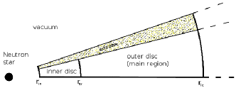
Figure 1: Schematic representation of our model (not to scale). We use $r_{\rm in}=10\,r_{\rm g}$ and $r_{\rm tr}=22\,r_{\rm g}$. For a $10$ ms pulsar (with mass $1.4\,M_{\odot}$), $r_{\rm cor}=18.8\,r_{\rm g}$ and $r_{\rm lc}=115\,r_{\rm g}$. The opening angles are $8^{\circ}$ for the disc alone and $10^{\circ}$ for the disc plus corona. The dashed lines indicate that the outer disc extends much further out than the main region shown here: the grid continues until $r_{\rm out}=380\,r_{\rm g}$ when we are solving for the toroidal component of the magnetic field and to $750\,r_{\rm g}$ when we are solving for the poloidal one.

3 Equations

In this section, we derive the equations for calculating the magnetic field structure and comment on the profile of the velocity field and on the turbulent diffusivity as well as saying something further about the boundary conditions. We also derive equations for calculating the magnetic torque exerted by the disc on the neutron star and briefly comment on the solution method.

3.1 Magnetic field

As mentioned previously, we are making our calculations using the kinematic approximation, within which the velocity field of the disc matter is specified separately (here following the K&K solution) rather than being solved for together with the magnetic field calculation. Once the velocity field has been specified, the magnetic field structure can then be obtained by solving the induction equation:

$$\partial_{t}\mathit{\mathbf{B}}=\nabla\times\left(\mathbf{v}\times\mathbf{B}-\eta\nabla\times\mathbf{B}\right)\,\,{\rm,}$$ (2)

where $\mathbf{B}$ and $\mathbf{v}$ are the mean components of the magnetic field and velocity field respectively, and $\eta$ is the turbulent magnetic diffusivity. Resolving the full structure of turbulence and studying accretion driven by the magneto-rotational instability goes well beyond the scope of this paper. Interested readers are referred to Romanova et al. (2011) where the first global axisymmetric simulations of that kind are described. Here, we use average quantities and follow a phenomenological approach for the angular momentum transfer. As in papers I and II, we are neglecting the so-called $\alpha$-effect, which involves the appearance of a large–scale electromotive force because of the interaction between the turbulent fluctuations in the magnetic fields and the velocity fields. This term creates a growing solution for the magnetic field and is fundamental when one wants to study dynamo effects. In line with our approach, we want to use a simple model where one can unambiguously understand the roles played by the different contributing factors. Only afterwards will additional ingredients (such as dynamo action) be added and their effects studied by comparison with the previous analyses.

We use spherical coordinates ($r$, $\theta$, $\phi$), with the origin of the coordinate system placed at the centre of the neutron star and the unit vector $\mathbf{\hat{z}}$ pointing in the direction of the magnetic dipole axis (and the stellar rotation axis). In our model we are assuming axisymmetry ($\partial_{\phi}[\dots]=0$) and we want to find a stationary solution ($\partial_{t}[\dots]=0$). The three scalar components of equation (2) are then:

$$0 = \partial_{\theta}\left\{\sin\theta\left[v_{r}B_{\theta}-v_{\theta}B_{r}-\frac{\eta}{r}[\partial_{r}(rB_{\theta})-\partial_{\theta}B_{r}]\right]\right\}\,\,{\rm,}$$ (3)

$$0 = \partial_{r}\left\{r\hskip 14.22636pt\left[v_{r}B_{\theta}-v_{\theta}B_{r}-\frac{\eta}{r}[\partial_{r}(rB_{\theta})-\partial_{\theta}B_{r}]\right]\right\}\,\,{\rm,}$$ (4)

$$0 = \partial_{r}\left\{r\left[v_{\phi}B_{r}-v_{r}B_{\phi}+\frac{\eta}{r}\partial_{r}(rB_{\phi})\right]\right\}-$$ (5)

$$\partial_{\theta}\left\{v_{\theta}B_{\phi}-v_{\phi}B_{\theta}-\frac{\eta}{r\sin\theta}\partial_{\theta}(B_{\phi}\sin\theta)\right\}\,\,\rm{.}$$

The first two equations are independent of $B_{\phi}$, and so we can solve these first for the poloidal components of the magnetic field and then solve the third equation afterwards for the toroidal component.

In order to solve for $B_{r}$ and $B_{\theta}$, one needs to specify profiles for $v_{r}$, $v_{\theta}$ and $\eta$ and to solve for $B_{\phi}$ one also needs a prescription for $v_{\phi}$. Then, given a set of consistent boundary conditions, the set of equations (3)–(5) has a single unique solution.

3.2 Velocity field

K&K made a calculation of the three-dimensional structure for an $\alpha$-disc, taking the disc to be suitably thin and Taylor expanding the equations of viscous hydrodynamics in terms of a small parameter $\epsilon\equiv\mathcal{H}/\mathcal{R}$, where $\mathcal{H}$ is a characteristic vertical scaleheight in the disc and $\mathcal{R}$ is a characteristic radius (taken, in practice, to be the radius of the neutron star). The equation of state of the accreting medium was taken to be polytropic with constant specific entropy, implying that for any comoving fluid element, increases in entropy due to viscous dissipation are exactly balanced by losses due to radiation and conduction. They were able to find analytical solutions for the lowest order terms in their Taylor expansions and these demonstrated a flow structure which was entirely an inward accretion flow at the top and bottom of the disc but could have an outward backflow near to the mid–plane at radii beyond a certain value. A similar flow pattern, including equatorial zone backflow, was found by Regev & Gitelman (2002) in a calculation including radiative transfer in an $\alpha$-disc modelled with a perfect gas equation of state. Clearly, this flow pattern is very different from that in standard S&S discs and so it was of interest to repeat our earlier calculations of magnetic field distortions by S&S discs also for these K&K ones.

The general form of the Taylor expansions used by K&K is given in section 2.1 of their paper. We use here their prescriptions for the poloidal components of the velocity field, $v_{r}$ and $v_{z}$, leaving the rotational velocity $\Omega$ as being Keplerian in the main part of the disc. Due to parity considerations and mass conservation, some of the terms appearing in the general form of the expansions are zero, and one is left with the leading-order terms in the expressions for $v_{r}$ and $v_{z}$ as being:

$$u=\frac{v_{r}}{\tilde{c}_{s}}=\epsilon\,u_{1}+\mathcal{O}(\epsilon^{3})\,\,{\rm,}$$ (6)

$$v=\frac{v_{z}}{\tilde{c}_{s}}=\epsilon^{2}\,v_{2}+\mathcal{O}(\epsilon^{4})\,\,{\rm,}$$ (7)

where $\tilde{c}_{s}$ is a characteristic sound speed in the disc. The analytic expressions for $u_{1}$ and $v_{2}$ are given by equations 2.53 and 2.56 of K&K, respectively.

For implementing this velocity field within our calculation, we first choose the geometrical profile of the disc by specifying the disc height $h$ as a function of radius $r$ (note that here we are using $h$ and $r$ to represent physical lengths and not the scaled quantities used in K&K). We choose this profile as being $h(r)=r\,\cos\theta_{\rm disc}$, where $\theta_{\rm disc}$ is the co-latitude of the disc surface (for which we take $\theta_{\rm disc}=82^{\circ}$). We sharply truncate the disc at an inner radius $r=r_{\rm in}$ (for which we take $r_{\rm in}=10\,r_{\rm g}$). We then specify a quantity which we call $v_{0}$, which is the value of the radial velocity $v_{r}$ at the point $(r_{\rm in},\theta_{\rm disc})$. Doing this turns out to be all that is required in order to uniquely determine the velocity field in physical units (i.e. as unscaled quantities). Changing the value of $v_{0}$ is equivalent to changing the value of $\alpha$. From equation 2.55 of K&K, one has (neglecting $\mathcal{O}(\alpha^{2})$ corrections):

$$v_{0}\simeq 2\,\alpha\,v_{K}\left(h/r\right)^{2}\,\,\rm{,}$$ (8)

where $v_{K}$ is the Keplerian linear velocity and all quantities are calculated at $(r_{\rm in},\theta_{\rm disc})$.

We follow the K&K poloidal velocity profile through all of the disc and then modify it in the corona. There we first modify $v_{\theta}$ via an error function in order to match the boundary conditions smoothly and analytically. Then we modify $v_{r}$ in such a way that the total local kinetic energy remains constant. The resulting velocity-field vectors are shown in Figs 2 and 3. Note the appearance of a ‘stagnation surface’ where both $v_{r}$ and $v_{\theta}$ go to zero, marking a change in direction of the flow. Having the surfaces where $v_{r}=0$ and $v_{\theta}=0$ coinciding is a particular property of the height profile that we are using here (with $h/r={\rm constant}$).

Figure 2: Velocity-field vectors $v_{r}$ and $v_{\theta}$ plotted using Cartesian coordinates $x$ and $z$ measured in units of the Schwarzschild radius. (Note that we use these Cartesian coordinates for plots throughout this paper.) The dashed line separates the inflow region from the backflow one. The heavy solid line marks the boundary between the corona and the external vacuum; the other solid line shows the boundary between the disc and the corona.

Figure 3: Magnification of Fig. 2 around the region where the flow changes direction. The region from $86^{\circ}$ to the equatorial plane is shown.

As regards the angular rotation velocity, we follow the same profile as in Paper II (see section 3.2 and fig. 2 of that paper). Here, we repeat the details again for completeness:

$$\Omega(r,\theta)=\left\{\begin{array}[]{cl}\Omega_{K}(r)&\hskip 8.5359pt\mbox{in the main region:}\\ &\hskip 8.5359pt\theta\in[\theta_{\rm disc},\pi/2],r\in[r_{\rm tr},r_{lc}]\\ &\\ \mbox{smooth join in $\theta$}&\hskip 8.5359pt\mbox{in the corona:}\\ &\hskip 8.5359pt\theta\in[\theta_{\rm cor},\theta_{\rm disc}]\\ &\\ \mbox{smooth join in $r$}&\hskip 8.5359pt\mbox{in the inner disc:}\\ &\hskip 8.5359ptr\in[r_{\rm in},r_{\rm tr}]\\ &\\ \Omega_{\rm s}&\hskip 8.5359pt\mbox{at the ghost zones: }\theta=\theta_{\rm cor}-\Delta\theta\\ &\hskip 8.5359pt\mbox{at the inner edge: }r=r_{\rm in}\end{array}\right.$$ (9)

where $\theta_{\rm cor}$ is the upper surface of the corona, $\Delta\theta$ is the angular grid resolution, $\Omega_{\rm s}$ is the stellar spin rate, $\Omega_{K}$ is the Keplerian angular velocity and the two smooth connections are made using the error functions given in equations (11) and (13) below.

In the $\theta$, direction we write

$$\tilde{\Omega}(r,\theta) = \Omega_{K}(r)\,f_{1}(\theta)+\Omega_{\rm s}\,[1-f_{1}(\theta)]$$ (10)

$$= [\Omega_{K}(r)-\Omega_{\rm s}]\,f_{1}(\theta)+\Omega_{\rm s}\,\,{\rm,}$$

where

$$f_{1}(\theta)=\frac{1}{2}\left[1+{\rm erf}\left(\frac{\theta-\theta_{\rm disc}}{\delta_{\theta}}\right)\right]\,\,{\rm,}$$ (11)

with $\delta_{\theta}=10^{-2}$ rad (i.e. $0.57^{\circ}$). Similarly, in the radial direction:

$$\Omega(r,\theta) = \tilde{\Omega}(r,\theta)\,f_{2}(r)+\Omega_{\rm s}\,[1-f_{2}(r)]$$ (12)

$$= [\tilde{\Omega}(r,\theta)-\Omega_{\rm s}]\,f_{2}(r)+\Omega_{\rm s}\,\,{\rm,}$$

where

$$f_{2}(r)=\frac{1}{2}\left[1+{\rm erf}\left(\frac{r-r_{\rm erf}}{\delta_{r}}\right)\right]\,\,{\rm,}$$ (13)

with $\delta_{r}=2\,r_{\rm g}$ and $r_{\rm erf}=14.4\,r_{\rm g}$.

This angular velocity profile is Keplerian in all of the outer disc (see Fig. 1), while in the corona and in the inner disc it deviates from Keplerian in order to match corotation at the boundaries. On the equatorial plane, $\Omega$ starts to become sub-Keplerian at $r_{1}=16.67\,r_{\rm g}$ (where deviations are of the order of $1\%$) and reaches its maximum at $r=15.18\,r_{\rm g}$, after which it decreases towards corotation.

3.3 Turbulent diffusivity

For the diffusivity, we follow the same approach as in Paper II, writing

$$\eta(r,\theta)=\eta_{0}\,\left\{1+\big{[}\eta_{\theta}(\theta)+\eta_{r}(r)\big{]}\,\left[\frac{\eta_{\rm c}}{\eta_{0}}-1\right]\right\}\,\,{\rm,}$$ (14)

where $\eta_{0}$ is the value in the main disc region and $\eta_{\rm c}$ is the value in the corona and inner disc (see Fig. 1). We here take $\eta_{0}=10^{10}$ cm² s^-1 and $\eta_{\rm c}=10^{12}$ cm² s^-1 as standard values. The magnitude of the diffusivity is often discussed in terms of the turbulent magnetic Prandtl number, which links it with that of the turbulent viscosity. There is a lot of uncertainty about which values to take and the one used here as our standard for $\eta_{0}$ may seem rather low. We have already discussed this issue in Paper II and note also the discussions by Reyes-Ruiz & Stepinski (1996) and others. We chose our value because it gives an interesting amount of field distortion in the disc, but it is clearly important to investigate the effects of varying it, and we also discuss this in the following sections.

For joining $\eta_{\theta}(\theta)$ and $\eta_{r}(r)$ between the low–$\eta$ and high–$\eta$ regions, we use joining functions of the form

$$f(x)=\frac{1}{2}\left[1+{\rm erf}\left(\frac{-x+x_{c}}{d_{x}}\right)\right]\,\,{\rm,}$$ (15)

where $x=\theta$ and $r$ for $\eta_{\theta}$ and $\eta_{r}$ respectively, with $x_{c}=\theta_{\rm disc}$ and $r_{\rm tr}$ in the two cases; $d_{x}$ is the width of the transition in the error function, for which we use $d_{r}=5\,r_{\rm g}$ in the radial direction and $d_{\theta}=2^{\circ}$ in the theta direction.

3.4 Boundary conditions

We have already commented on the boundary conditions being used for the present stages of our calculations: vacuum everywhere outside of the disc (plus corona) and the neutron star, with a dipolar magnetic field throughout those vacuum regions. This is highly idealized, of course, but it is our working approximation for the moment. In order to have a smooth transition between the disc and the external vacuum, we include a boundary layer, a corona, and then impose boundary conditions at the top of it. We also impose dipole conditions at the inner and outer radial edges of the disc. At the inner edge, this is done because the magnetic field is strong there and so it is very hard to get any distortions there at all. What is done at the outer edge is irrelevant anyway because we are placing it so far away that it does not influence what is happening inside the light cylinder, and so we make the simple choice of imposing dipole conditions there as well. In Paper I, we tested various kinds of boundary conditions (spherical lines, vertical lines and lines with $45^{\circ}$ inclination) and found that for poloidal magnetic field lines entering the extended disc (i.e. disc plus corona) at the same locations, their shape within the disc varied hardly at all among the different cases. However, the values for the field strength as a function of distance out along the surface of the extended disc will also vary depending on the structure of the external magnetic field and this will clearly influence the magnitude of the magnetic torque exerted by the disc.

We assume equatorial symmetry as well as axisymmetry and solve for only one quadrant. At our lower boundary in $\theta$ (i.e. at the equatorial plane), we require $B_{\theta}$ to be symmetric about the equatorial plane (i.e. $\partial_{\theta}B_{\theta}|_{\theta=\pi/2}=0$), while $B_{r}$ and $B_{\phi}$ have antisymmetric conditions there (i.e. $B_{r}$ and $B_{\phi}$ are zero at this boundary, and at the first ghost grid-point beyond it they have values opposite to those at the last active grid-point before it).

As regards the poloidal component of the velocity field, we follow K&K exactly for the inner and lower boundaries. This means that on the equatorial plane $v_{\theta}=0$ and $v_{r}$ is symmetric. This condition is equivalent to choosing a profile for $B_{\theta}$ at $\theta=\pi/2$ satisfying:

$$B_{\theta}(r,\pi/2)\,\,r\,\,v_{r}(r,\pi/2)={\rm const}\,\,{\rm.}$$ (16)

At the top boundary, we have to modify the K&K profile. In Paper I (section 3.2), we have already shown that if one requires the magnetic field to be a dipole, then the induction equation gives the following two conditions for the velocity field:

$$v_{\theta}=(v_{r}/2)\tan\theta\,$$ (17)

$$\Omega\propto r^{-\gamma/2}\sin^{\gamma}\theta\,\,{\rm,}$$ (18)

where $\gamma$ can take any value. We use the first condition directly to calculate $v_{\theta}$ in the coronal layer and for $\Omega$ we use corotation, which is consistent with the second condition with $\gamma=0$.

3.5 Torque calculation

The magnitude of the torque exerted by the accreting matter on the neutron star, is clearly affected by the behaviour of the magnetic field in the magnetosphere. In the present simple model, we are taking vacuum above and below the extended disc so that the magnetic field there remains strictly dipolar, but in the general realistic case there can be field-line inflation, as mentioned earlier, which may also lead to breaking of some of the magnetic linkage between the disc and the star. It has been suggested that associated opening of field lines might give rise to jets and winds: see, for example, Zanni & Ferreira (2013) concerning magnetospheric ejections. In this subsection, we consider the various contributions to the torque, first giving a rather general discussion and then specializing it to our simplified model.

3.5.1 General discussion

The disc can exert a torque on the central object via the link provided by magnetic field lines anchored at one end to the neutron star while the other end threads the disc, where the interaction with the moving matter creates a Lorentz force which can have a non-zero moment with respect to the central object. We call this contribution to the total torque $\mathbf{T}_{B-{\rm disc}}$.

As matter moves inwards, it encounters a progressively stronger magnetic field which eventually comes to completely dominate the motion of the plasma. This happens at the inner edge of the disc, where we suppose that matter leaves the disc following the magnetic field lines. If the magnetic field is then rigidly connected with the neutron star, it will force the matter to move with the same angular velocity as the central object. However, during this motion along the magnetic field lines, the matter is approaching the neutron star, and so although its angular velocity remains constant, there is a progressive decrease in its angular momentum (the cylindrical radial distance is decreasing). This occurs due to a torque exerted on it by the magnetic field lines, associated with which there is an equal and opposite torque tending to spin up the neutron star. We call this contribution $\mathbf{T}_{B-{\rm acc}}$.

Finally, when the accreting matter hits the neutron star surface, it transfers its residual angular momentum to the star. The torque concerned in this is typically very small, however, and we will neglect it here.

The total torque exerted on the star can then be written as:

$$\mathbf{T}_{\rm NS}=\mathbf{T}_{B-{\rm disc}}+\mathbf{T}_{B-{\rm acc}}\,\,{\rm,}$$ (19)

with

$$\mathbf{T}_{B-{\rm disc}} = \int\limits_{V}\mathbf{\tau}_{B-{\rm disc}}\,dV=-\int\limits_{V}\mathbf{r}\times\mathbf{F}_{\rm L}\,dV\,{\rm,}$$ (20)

$$\mathbf{T}_{B-{\rm acc}} = \dot{m}\,\frac{2\pi}{P_{\rm NS}}\,\left(\varpi_{\rm in}^{2}-\varpi_{\rm surf}^{2}\right)\,\mathbf{\hat{z}}\,\,{\rm,}$$ (21)

where $\mathbf{\tau}_{B-{\rm disc}}$ is the moment of the Lorentz force ($-\mathbf{F}_{\rm L}$) exerted on the neutron star by the local fluid element; $V$ is the volume containing all of the fluid elements associated with the disc which are magnetically linked to the neutron star and for which $\mathbf{F}_{\rm L}$ is non-zero; $\dot{m}$ is the accretion rate; $P_{\rm NS}$ is the neutron star spin period; $\varpi_{\rm in}$ is the distance from the rotation axis to the inner edge of the disc, while $\varpi_{\rm surf}$ is the corresponding distance for the point where the matter hits the surface of the neutron star and $\mathbf{\hat{z}}$ is the unit vector along the rotation axis. To the best of our knowledge, this is the first work where the magnetic torque is calculated by computing the integral of the Lorentz force through the whole disc, i.e. by means of equation (20). In the usual approach, only the value at the disc surface is considered.

Throughout this work we express torques with respect to the star, i.e. a positive value means that the torque is spinning the star up, while a negative one produces spin down.

The sign of $\mathbf{T}_{B-\rm acc}$ is always positive: it always acts so as to spin the star up (positive torque) because the angular momentum of the matter is decreasing when going from the inner edge of the disc to the neutron star surface. The sign of $\mathbf{T}_{B-{\rm disc}}$, however, is not obvious until the calculations are performed (see equation 27 below) and in general it can be either positive or negative.

We now consider in more detail the contribution to the torque due to the integrated moment of the Lorentz force (i.e. that coming from equation 20).

We are calculating the torque with respect to the origin of the coordinate system, and so the radial component of the force has zero moment. The force acting along the $\theta$ direction is always perpendicular to the position vector and so, if it is non-zero, it will always give a non-zero torque along the $\phi$ direction. However, since this component is antisymmetric with respect to the equatorial plane (while the position vector is symmetric), the integral of its moment will be zero. The only non-zero contribution to the net torque comes from the moment of the $\phi$ component. If we use $\mathbf{r}$ to indicate the position vector, and write $\mathbf{F}_{L}=(F_{r}\,\mathbf{\hat{r}},F_{\theta}\,\mathbf{\hat{\theta}},F_{\phi}\,\mathbf{\hat{\phi}})$ with $\mathbf{\hat{r}}$, $\mathbf{\hat{\theta}}$ and $\mathbf{\hat{\phi}}$ being unit vectors in the $r$, $\theta$ and $\phi$ directions, we have

$$\mathbf{\tau}_{B-\rm disc} = -\mathbf{r}\times\left(F_{r}\mathbf{\hat{r}}+F_{\theta}\mathbf{\hat{\theta}}+F_{\phi}\mathbf{\hat{\phi}}\right)=-r\mathbf{\hat{r}}\times\left(F_{\theta}\mathbf{\hat{\theta}}+F_{\phi}\mathbf{\hat{\phi}}\right)\,\,{\rm,}$$ (22)

$$\mathbf{\tau}_{B-\rm disc} = r\,F_{\phi}\,\mathbf{\hat{\theta}}-r\,F_{\theta}\,\mathbf{\hat{\phi}}\,\,{\rm,}$$ (23)

$$\mathbf{T}_{B-{\rm disc}} = \int\limits_{V}r\,F_{\phi}\,\mathbf{\hat{\theta}}\,dV=-2\pi\iint\limits_{r\theta}r\,F_{\phi}\,\,\,r^{2}\sin\theta\,drd\theta\,\,\mathbf{\hat{z}}\,\,{\rm,}$$ (24)

where in the last equality we have changed the volume integral into three integrals over the three coordinate directions, integrated over $\phi$ (giving the $2\pi$ factor) and have explicitly written the direction of the torque as being along the vertical axis (this implies a change of sign because $\mathbf{\hat{\theta}}$ and $\mathbf{\hat{z}}$ have opposite directions).

From Maxwell’s equations in cgs Gaussian units, we can write the general expression for the Lorentz force per unit volume as

$$\mathbf{F_{L}}=\frac{1}{c}\mathbf{J}\times\mathbf{B}=\frac{\nabla\times\mathbf{B}}{4\pi}\times\mathbf{B}\,\,{\rm,}$$ (25)

whose $\phi$ component in spherical coordinates is

$$F_{\phi} = \frac{1}{4\pi}\frac{B_{\theta}}{r\,\sin\theta}\partial_{\theta}(B_{\phi}\,\sin\theta)+\frac{1}{4\pi}\frac{B_{r}}{r}\partial_{r}(B_{\phi}\,r)$$ (26)

$$-\frac{1}{4\pi}\frac{1}{r\sin\theta}\left(B_{\theta}\partial_{\phi}B_{\theta}+B_{r}\partial_{\phi}B_{r}\right)\,\,{\rm.}$$

When considering axisymmetric models (as we are doing here), the third term can be neglected. The second term is also usually neglected for thin disc models because it involves derivatives with respect to the radius, while the first one involves vertical derivatives. The strategy of this work is to fully consider both radial and vertical structure and so we keep both terms in the torque calculation. Substituting equation (26) into (24) one obtains

$$\mathbf{T}_{B-{\rm disc}}=\iint\limits_{r,\theta}\left\{-\frac{1}{2}\left[B_{\theta}\partial_{\theta}(B_{\phi}\,\sin\theta)+\right.\right.$$

$$\left.\vphantom{\frac{1}{2}}\left.B_{r}\partial_{r}(B_{\phi}\,r)\sin\theta\right]r^{2}\right\}drd\theta\,\,\mathbf{\hat{z}}\,\,{\rm.}$$ (27)

We write the torque as the sum of two contributions in order to facilitate the comparison with the thin disc models that neglect the radial term:

$$\mathbf{T}_{B-{\rm disc}}=\mathbf{T}_{B-{\rm disc}}^{\theta}+\mathbf{T}_{B-{\rm disc}}^{r}\,\,{\rm,}$$ (28)

with

$$\mathbf{T}_{B-{\rm disc}}^{\theta} = \iint\limits_{r,\theta}-\frac{1}{2}\left[B_{\theta}\,\partial_{\theta}(B_{\phi}\,\sin\theta)\,r^{2}\right]drd\theta\,\,\mathbf{\hat{z}}\,\,{\rm,}$$ (29)

$$\mathbf{T}_{B-{\rm disc}}^{r} = \iint\limits_{r,\theta}-\frac{1}{2}\left[B_{r}\partial_{r}(B_{\phi}\,r)\,r^{2}\sin\theta\,\right]drd\theta\,\,\mathbf{\hat{z}}\,\,{\rm.}$$ (30)

3.5.2 Application to the model considered in this paper

As we have mentioned earlier (see Section 2), in the inner part of the disc our kinematic approximation breaks down because the magnetic pressure becomes non-negligible there with respect to the gas pressure (although it still remains smaller than the gas pressure until $r_{\rm in}$ is reached). In this part of the disc, we expect the angular velocity to become sub-Keplerian and finally to reach corotation with the neutron star at $r_{\rm in}$. Since we cannot reproduce this profile self-consistently (because we are using the kinematic approximation and are not solving an equation of motion), we change the $\Omega$ profile by hand in that region, as described in Section 3.2. This should actually mimic the real situation rather well. For this region, instead of using equation (20) to calculate the torque contribution, we instead calculate the back reaction on the field lines corresponding to the angular momentum loss by the matter; this would then be expected to be mainly transmitted to the neutron star (although it could also go into a jet). We calculate this torque contribution as

$$\mathbf{T}_{\Omega}=\dot{m}\left(\Omega_{1}\,r_{1}^{2}-\Omega_{NS}r_{\rm in}^{2}\right)\,\,\,\mathbf{\hat{z}}\,\,{\rm,}$$ (31)

where $r_{1}$ is the location on the equatorial plane where the angular velocity differs from the Keplerian value by $1\%$ ($r_{1}=16.67\,r_{\rm g}$ with our model settings), and $\Omega_{1}$ is the vertically averaged value of the angular velocity at that radial location. More rigorously one should consider local values for $\dot{m}$ and $\Omega$ and integrate equation (31) over the vertical direction.

We then calculate the magnetic torque from the disc as the sum of two components:

$$\mathbf{T}_{B-{\rm disc}}=\mathbf{T}_{\Omega}+\mathbf{T}_{B}$$ (32)

where $\mathbf{T}_{\Omega}$ is given by equation (31) and $\mathbf{T}_{B}$ is given by equation (20) integrated from $r_{1}$ out to the point where the contribution to the integral becomes negligible. We calculate $\mathbf{T}_{B-{\rm acc}}$ from equation (21), taking $\varpi_{\rm in}$ as being the distance from the rotation axis to the uppermost part of the inner edge of the disc (i.e. $r_{\rm in}\sin 80^{\circ}$) and getting $\varpi_{\rm surf}$ (the corresponding distance for the point where the infalling matter hits the surface of the neutron star) by assuming that the matter concerned follows dipole magnetic field lines after leaving the inner edge of the disc; this then gives $\varpi_{\rm surf}=r_{\rm NS}\,\sin(80^{\circ})/2$.

3.6 Solution method

Equation (2) has been solved numerically using a Gauss–Seidel iterative scheme with an evenly spaced grid in $r$ and $\theta$. As in papers I and II, all variables and coordinates were written in a dimensionless form for the purposes of the calculation. Because of the partial decoupling between the poloidal and toroidal components of the magnetic field, we have first solved for $B_{\rm pol}$ (measured in units of $B_{0}=3\times 10^{8}$ G), following the procedure described in Paper I, and then for $B_{\phi}$ (measured in units of $B_{\phi}^{0}=r_{0}^{2}\,B_{0}$, where $r_{0}=2.5$ is the radius of the neutron star in units of $r_{\rm g}$) following the procedure described in Paper II.

Details of the numerical scheme, including tests, have been given in papers I and II. From a technical point of view, the calculations performed here for obtaining the magnetic field structure are very similar to those of Paper II, the only difference being in the functions used for the velocity components. We recall that we use a grid resolution of $\Delta r=0.74\,r_{\rm g}$ and $\Delta\theta=0.125^{\circ}$ for both $B_{\rm pol}$ and $B_{\phi}$. In both cases, we use a numerical domain which is much larger than the physical domain of interest in order to avoid dependence of the results on the outer boundary conditions.

In addition to solving for the magnetic field structure, in this paper we are also solving for the torque, which involves calculating the integral given in equation (27). We do this by using a trapezoidal scheme, as described in Section 5.1.

4 Magnetic field structure

We have studied a range of different models, so as to investigate the effect of varying parameters, but first we present results for a representative fiducial model to provide a standard against which to compare the others.

4.1 Fiducial configuration

Our fiducial run is characterized by intermediate values of the magnetic Reynolds numbers, that are defined as $R_{\rm m}\equiv l_{c}\,v_{c}/\eta_{c}$, where $l_{c}$, $v_{c}$ and $\eta_{c}$ are characteristic values for the length, velocity and diffusivity, respectively. For $l_{c}$, we take the radius of the inner edge of the disc (i.e. $l_{c}=10\,r_{\rm g}=4.136\times 10^{6}$ cm); for $\eta_{c}$, we take $\eta_{0}$, as defined above; for $v_{c}$, we take either a representative radial velocity (for which we use $v_{0}$, as defined earlier) or a representative azimuthal velocity (for which we use the value of $v_{\phi}$ at the corotation radius, which we denote as $v_{0\,\phi}$). Depending on which of these velocities is used, we get either the poloidal or toroidal magnetic Reynolds number ($R_{m}^{\rm pol}$ or $R_{m}^{\rm tor}$, respectively). For our neutron star model, $v_{0\,\phi}=4.88\times 10^{9}$ cm s^-1.

The values that we use for our fiducial run are $R_{m}^{\rm pol}=103$ and $R_{m}^{\rm tor}=5\times 10^{5}$, which we obtain by taking $v_{0}=10^{6}$ cm s^-1 and $\eta_{0}=4\times 10^{10}$ cm² s^-1. The resulting structure of the poloidal component of the magnetic field $B_{\rm pol}$ is shown in Fig. 4. In Fig. 5, we show the contour plot of the toroidal component $B_{\phi}$. We find significant deviations of both $B_{\rm pol}$ and $B_{\phi}$ from the profiles which are usually considered, i.e. a dipole and the one given in equation (1), respectively.

Figure 4: Poloidal field lines for the fiducial run. The dot–dashed lines are dipole field lines, shown for comparison; the dashed line is the boundary between the corona and the disc; the dotted line is the stagnation surface.

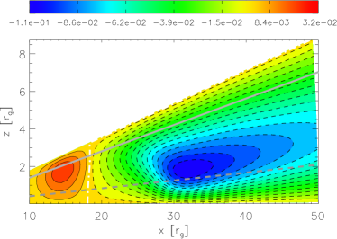
Figure 5: $B_{\phi}$ contour plot for the fiducial run, in units of $B_{\phi}^{0}$. Solid contours indicate positive values, while dashed lines are used for the negative ones. The solid grey line is the boundary between the disc and the corona; the dashed grey line here marks the stagnation surface and a white dot–dashed line is used for the zero-level contour (which is just inwards of the corotation point).

The reason for the deviations of $B_{\rm pol}$ away from the dipole are clear: when field lines enter the disc, they are pushed inwards by the inward motion of the plasma and a negative $B_{r}$ appears. As one moves towards the equatorial plane, the radial component of the velocity field decreases, goes through the stagnation surface and then becomes positive in the region of backflow (as shown in Fig. 3). As a consequence, we see that the magnetic field lines are bent backwards, with $B_{r}$ going through a zero and then becoming positive again. In the inner disc region, the magnetic field follows the plasma motion to a lesser degree, as it should if one assumes that the magnetic stresses eventually truncate the disc (in fact $B_{r}$ always stays positive in this region). We recall that we obtain this effect because in this region we have a larger characteristic value for the turbulent diffusivity (giving a smaller local magnetic Reynolds number).

The toroidal component of the magnetic field has two extrema: the first being positive and inwards of the corotation radius, and the second being negative and outwards of it. This is exactly what one would expect if $B_{\phi}$ were to follow equation (1), with the vertical field being the same as for a dipole. However, if one analyses the profile in more detail one sees that while the first peak follows closely that of $B_{\theta}\,\Delta\Omega$, the second one appears at a much larger radius. A similar behaviour was also obtained in Paper II and it was explained there by considering the magnetic distortion function $D_{m}$ (see section 5.2 of that paper). The distortion function was introduced in Paper I: it is defined in the same way as the magnetic Reynolds number but, instead of taking characteristic values for the velocity and the diffusivity, it takes local values. Depending on which velocity component one considers, one can have a poloidal or toroidal magnetic distortion function:

$$D_{\rm m}^{\rm pol} = \frac{r_{\rm g}\sqrt{v_{r}^{2}+v_{\theta}^{2}}}{\eta}\,,$$ (33)

$$D_{\rm m}^{\rm tor} = \frac{r_{\rm g}{v_{\phi}}}{\eta}\,\,{\rm.}$$ (34)

As in Paper II we find that the position of the second peak in $B_{\phi}$ follows the peak in the distortion functions (see Figs. 6 and 7).

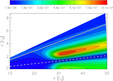
Figure 6: Contour plot of $D_{m}^{\rm pol}$. Its peak is at about the same radial location as that of $D_{m}^{\rm tor}$ (see Fig. 7), and that of the second peak in the $B_{\phi}$ contour plots (see Figs. 5, 12 and 13).

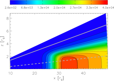
Figure 7: Contour plot of $D_{m}^{\rm tor}$. Its peak is at about the same radial location as that of $D_{m}^{\rm pol}$ (see Fig. 6), and that of the second peak in the $B_{\phi}$ contour plots (see Figs. 5, 12 and 13).

In Fig. 8, we report the shell averages of the poloidal component of the magnetic field calculated in half of the disc, with the dipole ones for comparison. Distortions are present in both poloidal components, with the ones for $B_{r}$ being the more evident. This component even changes sign, at about $x\sim 26$ (the absolute value of the shell average is being plotted) and stays negative from that radius outwards, tending to zero from negative values. For the $\theta$ component (whose intensity is larger by about one order of magnitude), there is a weak but extended amplification in the inner part, between $x=20$ and $x=30$. This is the region where magnetic field lines accumulate (see Fig. 4). We have seen the same behaviour also in papers I and II and it is what one might expect in the transition region, where the magnetic field goes from being dominated by the plasma (large distortions) to dominating over the plasma (small distortion, dipole field).

Figure 8: Shell averages for the poloidal components of the magnetic field: $B_{r}$ (dotted) and $B_{\theta}$ (solid). $B_{r}$ changes sign at $x\sim 26$. A dipole field is shown for comparison: its $r$ component is shown with the dot–dashed line, while its $\theta$ component is shown with the dashed line.

Fig. 9 compares the $B_{\phi}$ shell average with the results of Wang (1987) and Campbell (1987) and includes also the analytic prescription suggested in Paper II (see section 5.3 of that paper) that we report here for clarity:

$$B_{\phi}=\frac{r_{g}^{2}}{r\,\eta}\left[\partial_{r}(r\,v_{\phi}\,B_{r})+\partial_{\theta}(v_{\phi}\,B_{\theta})\right]\,\,{\rm.}$$ (35)

If we apply this expression to the model considered in the present calculation, the agreement is not as good as it was in Paper II. This is due to the breaking down of one of the assumptions made in deriving equation (35). In Paper II, we assumed that the $B_{\phi}$ generation rate $\partial_{t}\,B_{\phi}|_{+}$ can be written as $[\partial_{r}(r\,v_{\phi}\,B_{r})+\partial_{\theta}(v_{\phi}\,B_{\theta})]/r$ and that the loss term $\partial_{t}\,B_{\phi}|_{-}\,$ can be written as $\,\eta B_{\phi}/r_{\rm g}^{2}$ and we then equated the two terms (because we were looking for a stationary solution). In the present model, there are some regions of the disc where the approximation for the loss term represents only a lower estimate. Nevertheless, in Fig. 9, one can see that the analytic expression still has a similar behaviour to that of the numerical solution and the agreement is quite good in the interpeak region, although it overestimates $B_{\phi}$ in the inner part and underestimates it in the outer one. All of the curves have the same general behaviour, with two peaks (the first positive and inwards of corotation, the second negative and outwards of corotation), and they all go through zero at approximately the same location (close to the corotation point). However, the relative amplitudes of the two extremal points are very different. The models of the 1980s, i.e. equation (1) with a dipole $B_{z}$, predict the first (positive) peak to be the strongest one, whereas our present calculations are showing just the opposite, with the second (negative) peak having an amplitude more than four times larger than the first one. Our analytic prescription can reproduce this behaviour, with the ratio between the amplitudes of the second and first peaks being larger than $1$, although that is still smaller (i.e. $\sim 1.6$) than what is required.

Figure 9: Shell averages for the toroidal component: the solid line is the result for our fiducial configuration; the dashed line is the prediction of equation (1) with a dipole $B_{z}$ and the dotted line is our analytic prescription as obtained in Paper II and reported in equation (35). The scale for the fiducial shell average is given on the left y-axis, while the other two curves are normalized to the maximum of their absolute value (scale on the right). The 1980s result has its zero for $B_{\phi}$ at corotation ($\sim 19\,r_{\rm g}$), whereas the fiducial configuration has it at $\sim 17\,r_{\rm g}$ and the analytic profile has it at $\sim 16\,r_{\rm g}$.

4.2 Other configurations

4.2.1 List

In addition to the fiducial case, we analysed a range of other models to investigate the changes occurring in the magnetic field distortions when the parameters $v_{0}$ and $\eta_{0}$ (or $R_{m}^{\rm pol}$ and $R_{m}^{\rm tor}$) were varied over a wide range. Overall, we considered $13$ configurations, which we label ‘Mf’ to denote Magnetic field structure. These are all listed in Table 1. For each configuration, we report the value of the turbulent magnetic diffusivity, $\eta_{0}$, the scale factor of the velocity field in the poloidal direction, $v_{0}$, the poloidal magnetic Reynolds number, $R_{m}^{\rm pol}$, the toroidal magnetic Reynolds number, $R_{m}^{\rm tor}$, and the value of $\alpha$ corresponding to $v_{0}$ (see equation (8)).

Table 1: Parameter values for the Mf configurations.

Model	$\eta_{0}$	$v_{0}$	$R_{m}^{pol}$	$R_{m}^{tor}$	$\alpha$
	$(\rm{cm}^{2}\,\rm{s}^{-1})$	$(\rm{cm}\,\rm{s}^{-1})$
Fiducial	$4\times 10^{10}$	$10^{6}$	$1.03\times 10^{2}$	$5\times 10^{5}$	$3.8\times 10^{-3}$
Mf 1	$10^{10}$	$10^{6}$	$4.14\times 10^{2}$	$2\times 10^{6}$	$3.8\times 10^{-3}$
Mf 2	$10^{11}$	$10^{6}$	$4.14\times 10^{1}$	$2\times 10^{5}$	$3.8\times 10^{-3}$
Mf 3	$10^{12}$	$10^{6}$	$4.14$	$2\times 10^{4}$	$3.8\times 10^{-3}$
Mf 4	$10^{10}$	$10^{4}$	$4.14$	$2\times 10^{6}$	$3.8\times 10^{-5}$
Mf 5	$10^{10}$	$10^{5}$	$4.14\times 10^{1}$	$2\times 10^{6}$	$3.8\times 10^{-4}$
Mf 6	$10^{10}$	$2.5\times 10^{5}$	$1.03\times 10^{2}$	$2\times 10^{6}$	$9.4\times 10^{-4}$
Mf 7	$10^{9{\phantom{0}}}$	$0$	$0$	$2\times 10^{7}$	$0$
Mf 8	$10^{10}$	$0$	$0$	$2\times 10^{6}$	$0$
Mf 9	$10^{11}$	$0$	$0$	$2\times 10^{5}$	$0$
Mf 10	$10^{9{\phantom{0}}}$	$10^{5}$	$4.14\times 10^{2}$	$2\times 10^{6}$	$3.8\times 10^{-4}$

Configurations Mf 1 – Mf 3 differ from the fiducial case only in the value of $\eta_{0}$; the following three all have $\eta_{0}=10^{10}$ cm² s^-1 but different values of $v_{0}$; configurations Mf 7 – Mf 9 all have $v_{0}=0$ and $\eta_{0}$ ranging from $10^{9}$ to $10^{11}$ cm² s^-1; Mf 10 differs from Mf 1 in the values of $\eta_{0}$, $v_{0}$ and also $v_{0\,\phi}$ (not reported in the table), but has the same magnetic Reynolds numbers as Mf 1. The characteristic velocity $v_{0\,\phi}$ is the same ($4.88\times 10^{9}$ cm s^-1) for all of the configurations except for the last one, where we artificially lowered this value by a factor of $10$. In this case, therefore, the profile was no longer Keplerian. We were interested in this model because we wanted to test two cases which have different $\eta$ and $v$ (both poloidal and toroidal), but the same Reynolds numbers (Mf 1 and Mf 10).

4.2.2 Results

In Paper I we saw that what really matters for the poloidal field structure is the ratio between $v_{0}$ and $\eta_{0}$ (recall that in this paper $v_{0}$ is proportional to the disc $\alpha$, see Section 3.2). This is confirmed in the present calculations and, in fact, configurations with the same $R_{m}^{\rm pol}$ (i.e. Mf 3 and Mf 4; Mf 1 and Fiducial; Mf 2 and Mf 5; Mf 7, Mf 8 and Mf 9) give identical $B_{\rm pol}$. When $R_{m}^{\rm pol}$ increases (i.e. when $v_{0}$ increases or $\eta_{0}$ decreases) the field gets progressively more frozen-in with the fluid and therefore distortions grow as well (see Fig. 10). As shown in Fig. 11, this is clear also when comparing the shell averages. In the opposite regime instead (smaller $R_{m}^{\rm pol}$), the field tends to diffuse more, and deviations away from the dipole field are less evident (recall that we are imposing dipole boundary conditions). Configurations with high $R_{m}^{\rm pol}$ can lead to strong accumulation of magnetic field lines near to the inner edge of the disc. This magnetic field enhancement could favour jet-launching mechanisms, see e.g. Lii et al. (2012).

Figure 10: Poloidal magnetic field lines for configurations with $R_{m}^{\rm pol}=414$, i.e. Mf 1 and Mf 10.

Figure 11: Shell average of the poloidal magnetic field components $B_{r}$ (dotted) and $B_{\theta}$ (solid) for configurations with $R_{m}^{\rm pol}=414$, i.e. Mf 1 and Mf 10. $B_{r}$ changes sign at $x\sim 19$. Dipolar quantities are plotted for comparison: the dot–dashed line is the shell average of the radial component, the dashed line is that for the $\theta$ component.

Not surprisingly, this description does not suit the toroidal component as well, i.e. we see that configurations with the same ratio $v_{0}/\eta_{0}$ do not give the same $B_{\phi}$ values, but instead one should further consider $v_{0\,\phi}$. This is why we introduce the toroidal magnetic Reynolds number. In order to give the same profile for $B_{\phi}$ two configurations must have the same values of both $R_{m}^{\rm pol}$ and $R_{m}^{\rm tor}$. We show contour plots of $B_{\phi}$ for different pairs of the magnetic Reynolds numbers in Figs. 12 and 13. The structure of the toroidal component of the magnetic field does not change very much with varying $R_{m}^{\rm pol}$, even for $R_{m}^{\rm pol}=0$. When $R_{m}^{\rm pol}$ is held fixed and $R_{m}^{\rm tor}$ is varied, we find that $R_{m}^{\rm tor}$ affects only the scale factor for $B_{\phi}$ and that the shape of the contours is indeed determined only by $R_{m}^{\rm pol}$.

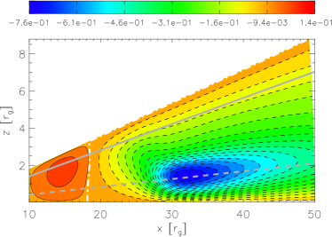
Figure 12: Contour plot of $B_{\phi}$, in units of $B_{\phi}^{0}$. Positive levels are plotted with solid lines, negative levels with dashed lines. The solid grey line indicates the boundary between the disc and the corona; the dotted grey line marks the stagnation surface; while the white dot–dashed line is used for zero contour levels. This result is for configurations with $R_{m}^{\rm pol}=414$ and $R_{m}^{\rm tor}=2\times 10^{6}$, i.e. Mf 1 and Mf 10.

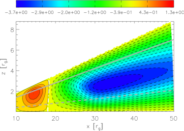
Figure 13: As in Fig. 12 but for configuration Mf 7, i.e. $R_{m}^{\rm pol}=0$ and $R_{m}^{\rm tor}=2\times 10^{7}$. Note that the negative peak is here higher up in the disc than it was in Figs. 5 and 12.

The behaviour described above is a consequence of the partial decoupling of the three components of the induction equation. As noted in papers I and II, under the assumptions of our models (i.e. axisymmetry, kinematic approximation and zero $\alpha$-effect), the $r$ and $\theta$ components of the mean field induction equation do not depend on any $\phi$ quantity, and so we find that the $B_{\rm pol}$ structure depends only on $R_{m}^{\rm pol}$. The $\phi$ component instead depends on both toroidal and poloidal quantities, and so we find that $B_{\phi}$ depends on both $R_{m}^{\rm pol}$ and $R_{m}^{\rm tor}$.

As a final test for this description we ran a calculation for a case (Mf 10) which has the same pair of Reynolds numbers as Mf 1, but given by different values of the three quantities $\eta_{0}$, $v_{0}$ and $v_{0\,\phi}$. As expected, we obtained identical results for the two cases.

5 Torque exerted on the neutron star

5.1 Torque from the disc

In this paper, we have been concerned mainly with investigating the structure of the magnetic field within our extended disc, when simple dipolar boundary conditions are applied at the top and bottom of it, and we have seen features which are quite interesting (and which we will discuss further in the next section). Other additional elements still remain to be added to our model before it will be fully ready to be used for realistic application to spin up rates of millisecond pulsars. However, following our discussion in Section 3.5, it is useful to already apply the formulae there to calculate preliminary torque estimates for our present model, both from the point of view of providing a suitable benchmark against which to compare subsequent more complete results and also because this turns out to highlight some aspects which can have more general relevance.

The torque exerted by the disc on the star via the magnetic field is expressed by equations (27) and (31). The second of these can be calculated analytically, while the first one is calculated by using our numerical results for the magnetic field components. Along the radial direction, we integrate from where the angular velocity deviates from the Keplerian profile by $1\%$ (at $r_{1}=16.67\,r_{\rm g}$) out to the point where the contribution to the integral becomes negligible, while along the $\theta$ direction we integrate over half the domain, from $80^{\circ}$ to $90^{\circ}$, and multiply by $2$ because of the symmetry. We use the same grid as that used for solving the induction equation (which is the grid where our solution for the magnetic field is defined) and use a trapezoidal scheme for two-dimensional quadratures, whose error is of the order of $O(\Delta r^{2})+O(\Delta\theta^{2})$. Given that $\Delta r=0.74\,r_{\rm g}$, $\Delta\theta=2.2\times 10^{-3}$ rad, and the integration range over $r$ and $\theta$ is $105\,r_{g}$ and $0.175$ rad respectively, we have a relative error of the order of $0.02\%$.

5.1.1 List of configurations

We have calculated the torque for all of the configurations considered so far. However, that set of configurations was chosen for investigating the effect on magnetic field distortions of varying the parameters and is not ideally suited for studying in detail how the torque depends on the Reynolds numbers. Because of this, we define here 16 additional configurations, which are listed in Table 2 and are labelled ‘To’ for Torque. As in Table 1, for each configuration, we report the values of the turbulent magnetic diffusivity, $\eta_{0}$, the representative velocity in the poloidal direction, $v_{0}$, the two magnetic Reynolds numbers, $R_{m}^{\rm pol}$ and $R_{m}^{\rm tor}$ and the parameter $\alpha$.

Table 2: Parameter values for the configurations of the To group.

Model	$\eta_{0}$	$v_{0}$	$R_{m}^{pol}$	$R_{m}^{tor}$	$\alpha$
	$(\rm{cm}^{2}\,\rm{s}^{-1})$	$(\rm{cm}\,\rm{s}^{-1})$
To 1	$10^{10}$	$2.5\times 10^{2}$	$1.03\times 10^{-1}$	$2\times 10^{6}$	$9.4\times 10^{-7}$
To 2	$10^{10}$	$2.5\times 10^{3}$	$1.03$	$2\times 10^{6}$	$9.4\times 10^{-6}$
To 3	$10^{10}$	$2.5\times 10^{4}$	$1.03\times 10^{1}$	$2\times 10^{6}$	$9.4\times 10^{-5}$
To 4	$10^{10}$	$1.75\times 10^{5}$	$7.24\times 10^{1}$	$2\times 10^{6}$	$6.6\times 10^{-4}$
To 5	$10^{10}$	$5.0\times 10^{5}$	$2.07\times 10^{2}$	$2\times 10^{6}$	$1.9\times 10^{-3}$
To 6	$10^{10}$	$7.5\times 10^{5}$	$3.10\times 10^{2}$	$2\times 10^{6}$	$2.8\times 10^{-3}$
To 7	$10^{10}$	$1.5\times 10^{6}$	$6.20\times 10^{2}$	$2\times 10^{6}$	$5.7\times 10^{-3}$
To 8	$10^{10}$	$1.75\times 10^{6}$	$7.24\times 10^{2}$	$2\times 10^{6}$	$6.6\times 10^{-3}$
To 9	$10^{10}$	$1.87\times 10^{6}$	$7.76\times 10^{2}$	$2\times 10^{6}$	$7.1\times 10^{-3}$
To 10	$10^{10}$	$2.0\times 10^{6}$	$8.27\times 10^{2}$	$2\times 10^{6}$	$7.6\times 10^{-3}$
To 11	$10^{10}$	$2.25\times 10^{6}$	$9.31\times 10^{2}$	$2\times 10^{6}$	$8.5\times 10^{-3}$
To 12	$10^{10}$	$3.75\times 10^{6}$	$1.55\times 10^{3}$	$2\times 10^{6}$	$1.4\times 10^{-2}$
To 13	$10^{11}$	$5\times 10^{6}$	$2.07\times 10^{2}$	$2\times 10^{5}$	$1.9\times 10^{-2}$
To 14	$10^{11}$	$1.87\times 10^{7}$	$7.76\times 10^{2}$	$2\times 10^{5}$	$7.1\times 10^{-2}$
To 15	$10^{11}$	$4.5\times 10^{7}$	$1.86\times 10^{3}$	$2\times 10^{5}$	$1.7\times 10^{-1}$
To 16	$10^{12}$	$10^{7}$	$4.14\times 10^{1}$	$2\times 10^{4}$	$3.8\times 10^{-2}$

Configurations To 1 – To 12 all refer to cases with $R_{m}^{\rm tor}=2\times 10^{6}$ and have $R_{m}^{\rm pol}$ varying between $\sim 10^{-1}$ and $\sim 1.5\times 10^{3}$. In order to keep the toroidal Reynolds number constant, we have to keep $\eta_{0}$ constant as well and get the change in the poloidal Reynolds number by changing only $v_{0}$. Configurations To 13 – To 15 have $R_{m}^{\rm tor}=2\times 10^{5}$ while the last one has $R_{m}^{\rm tor}=2\times 10^{4}$.

5.1.2 Results

The torque contributions from the inner part of the disc and from the accreting matter inwards of $r_{\rm in}$ are the same for all of our configurations, and can be calculated from equations (31) and (21). Inserting the characteristic values being used in this work, these give

$$\mathbf{T}_{\Omega}=1.379\times 10^{33}\,\,\mathbf{\hat{z}}\,[\rm{dyn\,cm}]\,$$ (36)

and

$$\mathbf{T}_{B-\rm acc}=0.646\times 10^{33}\,\,\mathbf{\hat{z}}\,\,[\rm{dyn\,\,cm}]\,{\rm.}$$ (37)

Note that both of these are positive (i.e. acting in the direction of tending to give spin-up of the neutron star). The torque from the rest of the disc, $\mathbf{T}_{B}$, is calculated as described above and can, in principle, be either negative or positive (although it is usually negative in practice). The total torque exerted on the neutron star, $T_{\rm NS}$, is then the sum of these three contributions.

A summary of results for the Mf and To configurations is shown in Tables 3 and 4, respectively. (We drop the vector notation for $\mathbf{T}$ from here on.) In the second and third columns, we give the contribution from the outer part of the disc, $T_{B}$ and the radial contribution to it, $T_{B}^{r}$ (see equation 28). Column four gives the total magnetic contribution from the disc ($T_{B-\rm{disc}}=T_{B}+T_{\Omega}$). The fifth column gives the total torque acting on the neutron star, i.e. $T_{\rm NS}=T_{B-\rm{disc}}+T_{B-{\rm acc}}$. Note that the term $T_{B}^{r}$, which is usually neglected in the thin disc approximation, is actually quite large here and in many cases acts to oppose $T_{B}^{\theta}$. Including $T_{B}^{r}$ in two-dimensional calculations of the magnetic torque is therefore very important. $T_{B}^{\theta}$ remains dominant for all of these configurations, however, except for those with the highest values of $R_{m}^{\rm pol}$ (giving the largest radial distortions).

Table 3: Values of the computed torque for the Mf configurations. $T_{B}$ is the torque due to the interaction between the magnetic field and the disc in the region outwards of $r_{1}$; $T_{B}^{r}$ is its radial component; $T_{B-{\rm disc}}$ is the magnetic contribution from all of the disc; $T_{\rm NS}$ is the total torque exerted on the neutron star. The torques are expressed in units of $10^{33}$ dyn cm, with positive values indicating that they are acting in the direction of spinning up the neutron star while negative values give spin-down.

Model	$T_{B}$	$T_{B}^{r}$	$T_{B-{\rm disc}}$	$T_{\rm NS}$
Fiducial	$-1.61$	$0.34$	$-0.23$	$0.41$
Mf 1	$-6.68$	$-5.12$	$-5.30$	$-4.66$
Mf 2	$-0.47$	$0.12$	$0.91$	$1.56$
Mf 3	$-0.03$	$0.01$	$1.35$	$1.99$
Mf 4	$-3.22$	$0.69$	$-1.84$	$-1.19$
Mf 5	$-4.66$	$1.16$	$-3.28$	$-2.64$
Mf 6	$-6.44$	$1.37$	$-5.07$	$-4.42$
Mf 7	$-30.4$	$6.27$	$-29.0$	$-28.35$
Mf 8	$-3.04$	$0.63$	$-1.66$	$-1.01$
Mf 9	$-0.30$	$0.06$	$1.08$	$1.72$
Mf 10	$-6.68$	$-5.12$	$-5.30$	$-4.66$

Table 4: As for Table 3 but for the To configurations.

Model	$T_{B}$	$T_{B}^{r}$	$T_{B-{\rm disc}}$	$T_{\rm NS}$
To 1	$-3.04$	$7.41$	$-1.66$	$-1.02$
To 2	$-3.08$	$7.37$	$-1.70$	$-1.06$
To 3	$-3.48$	$6.88$	$-2.10$	$-1.45$
To 4	$-5.65$	$4.04$	$-4.27$	$-3.62$
To 5	$-7.88$	$-0.16$	$-6.50$	$-5.86$
To 6	$-7.76$	$-1.73$	$-6.38$	$-5.74$
To 7	$-3.57$	$-1.49$	$-2.19$	$-1.54$
To 8	$-2.05$	$-0.72$	$-0.67$	$-0.02$
To 9	$-1.35$	$-0.30$	$0.03$	$0.67$
To 10	$-0.71$	$0.14$	$0.67$	$1.32$
To 11	$0.41$	$1.00$	$1.79$	$2.44$
To 12	$2.53$	$3.52$	$3.91$	$4.56$
To 13	$-0.79$	$0.01$	$0.59$	$1.24$
To 14	$-0.14$	$-0.03$	$1.24$	$1.89$
To 15	$0.14$	$0.26$	$1.52$	$2.17$
To 16	$-0.05$	$0.06$	$1.33$	$1.98$

In the usual description of the interaction between the magnetosphere and the disc, the sign of the torque caused by the magnetic field deformation is taken to be the same as that of $B_{\phi}$. However, this result follows after a succession of approximations have been made. In equation (27), which defines the magnetic torque, one can see that $B_{\phi}$ enters only via derivative terms. From the contour plots of $B_{\phi}$ (see Figs. 5, 12 and 13) it is clear that the sign of these does not always coincide with the sign of $B_{\phi}$ itself. This is why our results can be significantly different from those of the models developed in the 1980s (and subsequent calculations using a similar approach) and why we see changes in the sign of the magnetic torque without any change in the sign of $B_{\phi}$, but with only a modification of its two-dimensional structure (actually changes related to the poloidal component are larger here than those coming from the toroidal one). This aspect is considered further in Section 5.3 below, where we focus in particular on the question of which regions of the disc tend to spin the star up or down.

5.2 Dependence on the magnetic Reynolds numbers

Usually differences in the magnetic torque are caused by differences in the spin period of the star or in its magnetic field, but we have shown here that serious differences in the torque could also be caused by variations in the velocity field and the turbulent diffusivity, i.e. in the magnetic Reynolds numbers. We now want to describe better how this works.

We have already commented in Section 4.2.2 that $R_{m}^{\rm pol}$ fully determines the poloidal component of the magnetic field and $R_{m}^{\rm tor}$ enters as a scale factor in the toroidal component. Since the equation for calculating the magnetic torque is homogeneous in all of the magnetic field components (see equation 27), it was to be expected that $R_{m}^{\rm tor}$ would affect the torque only as a scale factor. The other Reynolds number, $R_{m}^{\rm pol}$, instead influences the shape of the magnetic field lines and it is not trivial to predict its effect on the torque. In order to analyse this, we consider configurations with the same $R_{m}^{\rm tor}$ and different $R_{m}^{\rm pol}$ and we then plot the torque against $R_{m}^{\rm pol}$.

Results are shown in Fig. 14, where the poloidal magnetic Reynolds number ranges from $0$ to $1.55\times 10^{3}$ and the toroidal one is kept fixed at $2\times 10^{6}$. In Fig. 14, we show both the total torque exerted on the neutron star and also the contribution coming from just the magnetic linkage with the disc, $T_{\rm B-disc}$. We have made similar calculations also for a different value of the toroidal magnetic Reynolds number, $R_{m}^{\rm tor}=2\times 10^{5}$ and found values for $T_{\rm B-disc}$ exactly a factor of 10 smaller, as expected.

Figure 14: Dependence of the torque on the poloidal magnetic Reynolds number $R_{m}^{\rm pol}$. Here, $R_{m}^{\rm tor}$ is fixed at $2\times 10^{6}$. The solid line shows the total torque exerted on the neutron star, while the dashed line is for $T_{B-\rm{disc}}$ alone. The leftmost point is for $R_{m}^{\rm pol}=0$ but is actually drawn at $10^{-2}$ so as to give a better visualization.

As one can see from Fig. 14, for very low $R_{m}^{\rm pol}$ the torque tends asymptotically to about $-1\times 10^{33}$ dyn cm. This means that when $B_{r}$ and $B_{\theta}$ are not distorted at all, i.e. the poloidal field is exactly a dipole, the disc still gives a magnetic contribution to the torque. This was of course expected, since one still has distortions in the $B_{\phi}$ component. Indeed, in most of the models in the literature, the poloidal field is assumed to be a dipole and yet the torque is non-zero. As deviations away from a dipole field increase (i.e. as $R_{m}^{\rm pol}$ increases), the torque becomes progressively more negative and reaches a minimum of $\sim-6\times 10^{33}$ dyn cm at $R_{m}^{\rm pol}\sim 200$. For even larger values of $R_{m}^{\rm pol}$, the torque starts to rise again and becomes positive.

Because of the proportionality between $R_{m}^{\rm tor}$ and $T_{B}$, we expect that as we lower $R_{m}^{\rm tor}$ the absolute value of $T_{B}$ will become progressively smaller. In particular, when $R_{m}^{\rm tor}$ reaches some critical value (say $R_{m}^{\rm zero}$) the negative peak in $T_{B}$ will be just enough to balance $T_{\Omega}+T_{B-{\rm acc}}$. In this case the total torque acting on the neutron star would always be positive except for the $R_{m}^{\rm pol}$ which gives the maximum torque, when it would instead be zero. When $R_{m}^{\rm tor}$ becomes smaller than a threshold value (say $R_{m}^{\rm const}$), $T_{B}$ would eventually become completely negligible with respect to $T_{\Omega}+T_{B-{\rm acc}}$ ($<1\%$), so that the total torque $T_{\rm NS}$ would be of the order of $2\times 10^{33}$ dyn cm for any value of $R_{m}^{\rm pol}$ or $\alpha$. By assuming that the linear scaling between $B_{\phi}$ and $R_{m}^{\rm tor}$ is valid for any $R_{m}^{\rm tor}$, we estimate these threshold values to be about $R_{m}^{\rm zero}=4\times 10^{5}$ and $R_{m}^{\rm const}=4\times 10^{4}$.

We should make a careful caveat here, however. This discussion has been made within the context of our present simplified model. Including the effects of line inflation would be expected to decrease the magnitude of $T_{B}$, making spin-up more likely.

5.3 Spin-up and spin-down regions

Finally, we would like to comment in detail on the regions of the disc that spin the star up or down. In previous work, there has been a widespread consensus that the part of the disc which is inwards of the corotation radius gives a spin-up contribution, while that which is outwards of the corotation radius gives a negative contribution.

In order to investigate this aspect, we have calculated the contribution to the magnetic torque at every location inside the disc (i.e. the local value of the integrand in equation (27)) and have then produced a contour plot of this magnetic torque density. The regions where it is negative act in the sense of spinning the star down, while those where it is positive act in the sense of spinning the star up. We have calculated this quantity for four key configurations, which have been chosen considering the behaviour shown in Fig. 14. They are: (i) configuration Mf 8 with zero $R_{m}^{\rm pol}$, (ii) configuration To 5 with the largest negative torque, (iii) configuration To 8 with roughly zero net torque and (iv) configuration To 12 with the largest positive torque. We have considered configurations with the same value of $R_{m}^{\rm tor}=2\times 10^{6}$ (since the torque scales with $R_{m}^{\rm tor}$ comparisons should be made keeping this quantity constant) and with $R_{m}^{\rm pol}<2\times 10^{3}$ (for larger values distortions are too large and could be non-realistic).

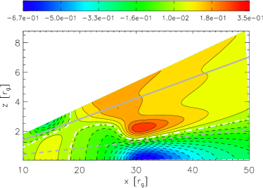
Figure 15: Contour plot of the magnetic torque density (the integrand in equation (27)) measured in units of $2.5\times 10^{35}$ dyn, for configuration To 5 with $R_{m}^{\rm pol}=207$ and $R_{m}^{\rm tor}=2\times 10^{6}$. As usual, contours of negative torque are drawn with dashed lines and those for positive torque are drawn with solid lines. Regions with positive torque act in the sense of spinning up the star, and those with negative torque act in the sense of spinning it down. The white dot–dashed curves are zero lines.

The contours for case (ii) are shown in Fig. 15. The most striking feature of this is the region of positive spin-up which at high latitudes extends over all radii from about the corotation point outwards, which is contrary to what is usually thought. A second relevant feature is that there is a clear vertical structure, with the upper part being the spin-up region. Inwards of the corotation radius the structure is reversed, with the equatorial region contributing to the spin-up and the upper part to the spin-down. We recall that our $\Omega$ profile is basically Keplerian from the outer edge of the disc up until $r_{1}=16.67\,r_{\rm g}$, inwards of which it is progressively changed so as to match with corotation at the inner edge of the disc.

The analysis of the torque density for the other three cases gives very similar results, with differences only in the details of the structure, e.g. the exact location of the boundary between the spin-up and spin-down regions. We have calculated the torque density also for the reference case of Paper II, i.e. model number $1$ in Table 5. We there again obtain spin-up regions also outside the corotation radius and see evidence of a vertical structure (in this case with two changes of sign as one moves from the corona towards the equatorial plane).

All of the cases show a strong relation between the magnetic torque density and the vertical structure of the toroidal component of the magnetic field. This can be seen more clearly if one compares the $B_{\phi}$ contour plot with the magnetic torque density plot. The sign of the torque density is opposite to that of the vertical derivative of the toroidal field $\partial_{\theta}B_{\phi}$, just as predicted by equation (27), when $T_{B}^{r}$ is smaller than $T_{B}^{\theta}$.

Figure 16: Shell average of the magnetic torque density for configurations To 8, To 5 and Mf 8. The solid line marks the zero level, which is shown as a reference.

We have calculated a shell average of the magnetic torque density over the upper half of the disc to obtain an estimate of the total contribution to the torque from the disc at any given radial location. Results are shown in Fig. 16 for cases (i) – (iii). This confirms that there are parts of the disc outwards of the corotation radius that spin the star up. Also, it shows that nothing special is happening for the magnetic torque at the corotation radius (at $18.8\,r_{\rm g}$). The toroidal magnetic field is zero there, but the magnetic torque depends only on the derivative terms.

6 Comparison with our earlier models

In papers I and II, we considered the distortion of the magnetic field when the Shakura and Sunyaev disc velocity profile was used. Table 5 lists some of the configurations described in Paper II (which we will often refer to as PII in this subsection). For each of them, we have now calculated the torque as described in Section 3.5 and the results of this are reported in Table 6.

Table 5: Values of the magnetic Reynolds numbers for those configurations of Paper II (PII) that are considered here. The last column reports some of the configurations of the current paper which have the same or similar magnetic Reynolds numbers.

Model	$\eta_{0}$	$v_{0}$	$R_{m}^{\rm pol}$	$R_{m}^{\rm tor}$	Close models
(PII)	$(\rm{cm}^{2}\,\rm{s}^{-1})$	$(\rm{cm}\,\rm{s}^{-1})$			Current paper
1	$\eta_{0}=10^{10}$	$10^{5}$	$41.4$	$2\times 10^{6}$	Mf 1, Mf 5
2	$\eta_{0}=4\times 10^{10}$	$10^{5}$	$10.3$	$5\times 10^{5}$	Fiducial, To 3
3	$\eta_{0}=10^{11}$	$10^{5}$	$4.14$	$2\times 10^{5}$	Mf 2 – 4
4	$\eta_{0}=10^{12}$	$10^{5}$	$0.41$	$2\times 10^{4}$	Mf 3, To 1,  2

Table 6: Values of the computed torque for the configurations of Paper II, where the S&S velocity profile was used. The quantities reported here are the same as in Tables 3 and 4.

Model	$T_{B}$	$T_{B}^{r}$	$T_{B-{\rm disc}}$	$T_{\rm NS}$
1	$-21.6$	$-17.0$	$-20.2$	$-19.6$
2	$-4.42$	$-2.45$	$-3.04$	$-2.39$
3	$-1.06$	$-0.05$	$0.32$	$0.97$
4	$-0.04$	$0.07$	$1.34$	$1.99$

There is no straightforward way of comparing between individual models in PII and the current paper. All of the models have a neutron star with the same mass and magnetic field, accreting at the same mass accretion rate and, in PII, even with the same $\alpha$-parameter. The poloidal velocity fields are instead very different. It seems best to consider the comparison in an overall sense. Although the Reynolds numbers are useful indicators, we cannot here expect models of the two types with the same pair of Reynolds numbers to give identical results, because these numbers depend on the magnitude of the velocity fields only at a specific location and do not take into account how the velocities change with position. (For the turbulent diffusivity, we are using the same profile as in PII.)

As regards the distortion of the magnetic field lines, in Section 4, we have seen that the distorted pattern is closely related to the behaviour of the fluid flow. Since in this paper we use a velocity field which is quite different from that in PII, we should not expect the poloidal magnetic field lines for the two cases to be similar. In PII, $v_{r}$ was always inward pointing, whereas now there is inflow at the higher latitudes but a backflow in the region of the mid-plane which is reflected in a bending backwards of the field lines in that region. In addition, the magnitude of the velocity field in the disc decreases strongly with increasing $\theta$ in the present calculations, whereas in PII it was constant. This strong decrease results in a weaker distortion for fixed $v_{0}$ and $\eta_{0}$.

For the toroidal direction, we use the same $\Omega$ profile in both papers. However $B_{\phi}$ and the magnetic torque also depend on the configuration of the poloidal magnetic field, so that even for configurations with the same $R_{m}^{\rm tor}$ (and $R_{m}^{\rm pol}$) we cannot expect to get the same results. In fact, the $B_{\phi}$ contours show an important difference, in that the large region of positive $B_{\phi}$ outside the corotation radius found in Paper II, is no longer present here. The velocity field is the origin of this difference (nothing else has changed); however, it is not trivial to isolate the specific aspect which is causing this feature to disappear. Probably, it is because, with the new velocity profile, the distortions of the vertical component $B_{\theta}$ are smaller than in papers I and II (compare for example Fig. 8 with fig. 4 of Paper I).

As regards the magnetic torque, we can make a more quantitative comparison. For every model in PII, we can find a configuration in this work which has the same $R_{m}^{\rm pol}$ (or is very close to it). We then consider the ratio of the $R_{m}^{\rm tor}$ for the Paper II model to that of this paper, and use this factor to scale the magnetic torque of the PII model. Results from doing this are reported in Table 7. In general, the torques for PII are larger than what we find in the current calculations (in absolute value). This can be explained by the larger distortions found in PII. In addition to being larger, the distortions also follow a different pattern, and so the relative contributions of the two terms in the torque, as introduced in equation (28), are very different. Having an equatorial backflow in the velocity field distorts the magnetic field in such a way that the two parts of the magnetic torque often act in opposite directions and so the total torque is smaller than when $T^{r}_{\rm B-disc}$ is neglected. With the S&S velocity field, where there is no flow reversal and $v_{r}$ is constant with $\theta$, the two terms tend to have the same sign, and therefore the total magnetic torque tends to be larger. However, the differences should progressively diminish for smaller and smaller $R_{m}^{\rm pol}$, because in the limit as $R_{m}^{\rm pol}\to 0$ the magnetic field tends to a dipole, regardless of the velocity field profile. This is nicely confirmed by the numbers in Table 7, where the ratio of the torques becomes smaller as $R_{m}^{\rm pol}$ decreases.

Table 7: Comparison between the torques found in the current work and in Paper II (PII). The first two columns show which models are being compared. The third column gives the value of the poloidal magnetic Reynolds number for the PII model. The last column gives the ratio between the scaled PII torque and the torque of the equivalent model in the current paper.

PII model	Current work model	$R_{m}^{\rm pol}$ PII	(Scaled $T_{B}^{\rm PII})/T_{B}$
1	Mf 5	41.4	4.6
2	To 3	10.3	5.1
3	Mf 3	4.14	3.3
3	Mf 4	4.14	3.7
4	To 1	0.41	1.3
4	To 2	0.41	1.3

7 Conclusions

This paper is part of a step-by-step analysis of the interaction between the magnetic field of a central rotating neutron star and an encircling accretion disc, focusing particularly on millisecond pulsars. Our strategy has been to start with a very simple model and then to progressively include additional features one at a time, so as to understand the effects of each of them. For the model presented here, we have considered a neutron star with a dipole magnetic field aligned with the rotation axis, surrounded by a disc which is truncated at the Alfvén radius and which has a coronal layer above and below it, treated as a boundary layer between the disc and its exterior. The external region is here taken to be vacuum and the magnetic field there is taken to be a perfect dipole. (Effects coming from interfacing on to a non-vacuum magnetosphere will be considered in subsequent work.) We have used the kinematic approximation, in which the velocity field of the matter is kept fixed, and have solved the induction equation for mean fields looking for a stationary configuration. We solve self-consistently for all of the magnetic field components, employing a velocity field having all three components different from zero, and do not neglect horizontal derivatives.

The code and the procedure used for this analysis have been described in detail in Naso & Miller (2010, 2011), where we used a specific three-dimensional extension of the Shakura & Sunyaev (1973) velocity profile (i.e. a velocity field with three non-zero components, each depending at most on the two coordinates $r$ and $\theta$). Here, instead, we consider a more general prescription for the velocity field, as described in Kluźniak & Kita (2000). The key features of this velocity field are (1) a fully three-dimensional axisymmetric profile and (2) the presence of a flow reversal (backflow) in a region close to the equatorial plane.

The magnetic configuration that we find is consistent with the conceptual picture described in papers I and II. As soon as magnetic field lines enter the corona, they start to be pushed inwards by the accreting matter. However, as one proceeds downwards in the disc, they start to be bent back again, as a consequence of the change in direction of the velocity field from inflow to backflow (see Fig. 4). When interaction with a non-vacuum magnetosphere is included, one expects to see the field lines above and below the disc being spread out with respect to the dipole configuration. It is interesting to compare our results with ones from those calculations which show this line inflation and also resolve the region inside the disc (e.g. Miller & Stone, 1997; Zanni & Ferreira, 2009; Romanova et al., 2011; Zanni & Ferreira, 2013); it can be seen that our solutions for the magnetic field-line structure inside the disc are rather similar to those.

The toroidal component of the magnetic field in our present calculations shows a simpler profile than that in Paper II (see Fig. 5). It is positive (dragged forwards with respect to the neutron star) inwards of the corotation point and negative (dragged backwards with respect to the neutron star) outwards of that, just as envisaged by Wang (1987) and Campbell (1987) (i.e. as given by equation 1 when a dipole field is used for $B_{z}$). However, we find some crucial differences with respect to those models: (1) the relative strength of $B_{\phi}$ at the two extrema is reversed and, most importantly, (2) $B_{\phi}$ decreases with $r$ much more slowly, and this has consequences for the torque (see Fig. 9).

We find it convenient to introduce two magnetic Reynolds numbers to describe the magnetic field structure. One, $R_{m}^{\rm pol}$, is defined using a characteristic poloidal velocity and the other one, $R_{m}^{\rm tor}$, uses the Keplerian linear velocity at the corotation point. The former fully determines the structure of $B_{\rm pol}$ and the shape of $B_{\phi}$, while the latter fixes the magnitude of $B_{\phi}$. It is only when two configurations have the same pair of Reynolds numbers that one obtains the same results for all of the three components of the magnetic field. When the profile of the velocity or of the magnetic diffusivity is changed, the magnetic Reynolds numbers lose their predictive power and one should instead consider the magnetic distortion functions $D_{m}^{\rm pol}$ and $D_{m}^{\rm tor}$ (i.e. a two-dimensional generalization of the magnetic Reynolds numbers), meaning that configurations with the same $R_{m}$ but different $D_{m}$ give different results. As in Paper II, we find that the magnetic distortion functions determine the position of the second peak in $B_{\phi}$; while the first peak is connected with $B_{\theta}\Delta\Omega$.

We have also made preliminary calculations of the total torque exerted on the neutron star. We split this into two parts: (1) the torque produced by the interaction between the magnetic field and the disc $T_{B-\rm disc}$ and (2) that produced by the accreting matter, leaving the disc at the inner edge and reaching the NS surface along magnetic field lines, $T_{B-{\rm acc}}$. The standard reference for calculating $T_{B-\rm disc}$ is Ghosh & Lamb (1979b). Here we have modified that approach in two ways: (1) we drop some of the simplifying assumptions made in calculating the analytic expression for the torque (i.e. we retain both horizontal and vertical derivatives) and (2) for the magnetic field we use our numerical results, rather than the approximated profile of earlier models, although we recall our caveats about our present neglect of line-inflation and possible breaking of magnetic linkage beyond a certain radius in the disc. Regarding the dipolar boundary conditions: in Paper I we showed that the shape of the field-lines inside the disc does not depend on the chosen boundary conditions. However, the magnitude of the field is affected, and the dilution introduced by line inflation would be expected to decrease the overall torque from the outer parts of the disc. (We will comment further on this below.) Regarding the breaking of magnetic linkage: we note that in the results of Zanni & Ferreira (2009), the point where magnetic linkage is lost comes at beyond twice their co-rotation radius. The situation which they are considering is rather different from ours (they are studying T Tauri stars), but if one transfers this result to our case, it would correspond to loss of linkage only at the very edge of the domain used in our plots, where the magnetic torque contribution is negligible anyway.

In the standard scenario developed in the 1980s and 1990s, and still widely used, the magnetic torque is taken to be proportional to $B_{\phi}$, which in turn is taken to be proportional to the difference between the local $\Omega$ of the disc matter and that of the central object, so that the disc inwards of the corotation radius gives a spin-up contribution, while the remaining part gives a spin-down. We find that this description, although rather reasonable, in fact fails to reproduce the behaviour of a simple two-dimensional disc model, even when the vertical averages of $B_{\phi}$ and the magnetic torque are considered (see Figs. 9 and 16). For any given configuration, there is a vertical structure, such that at any radius there are both spin-up and spin-down regions (at different heights in the disc, as shown in Fig. 15) whose locations vary with the values of the magnetic Reynolds numbers. The sign of the torque mainly follows that of the vertical derivative of the toroidal field, $\partial_{\theta}B_{\phi}$. We find similar results also when calculating the torque for the models of papers I and II, with an S&S velocity profile.

Within our present model, the torque contributions from the inner part of the disc and from the accreting matter inwards of its inner edge are both positive (acting in the sense of spinning up the neutron star) while that from the rest of the disc can be either positive or negative. We have shown that the behaviour of the latter is complicated, and needs to be calculated with care rather than relying on the standard simplified prescriptions. However, for our present restricted model, we find that the net contribution from this region would still be negative (acting in the direction of spin-down), except in extreme cases, and that it would generally dominate over the positive contributions. This cannot be right for the spinning-up of millisecond pulsars, and so we infer that the action of field-line inflation and reconnections in weakening the negative torque from the outer parts of the disc probably plays a crucial role in allowing the overall spin-up.

In this paper, we have extended our previous work, where we used the S&S velocity profile, by using instead the more sophisticated profile given by K&K, and we have also made calculations for the torque exerted by the disc on the neutron star. The next step of our programme of work will be to replace the present vacuum boundary conditions by a consistent treatment of the interface with a non-vacuum force-free magnetosphere.