Non-minimal Universal Extra Dimensions with Brane Local Terms: The Top Quark Sector

Abstract

We study the physics of Kaluza-Klein (KK) top quarks in the framework of a non-minimal Universal Extra Dimension (nmUED) with an orbifolded ($S^{1}/Z_{2}$) flat extra spatial dimension in the presence of brane-localized terms (BLTs). In general, BLTs affect the masses and the couplings of the KK excitations in a non-trivial way including those for the KK top quarks. On top of that, BLTs also influence the mixing of the top quark chiral states at each KK level and trigger mixings among excitations from different levels with identical KK parity (even or odd). The latter phenomenon of mixing of KK levels is not present in the popular UED scenario known as the minimal UED (mUED) at the tree level. Of particular interest are the mixings among the KK top quarks from level ‘0’ and level ‘2’ (driven by the mass of the Standard Model (SM) top quark). These open up new production modes in the form of single production of a KK top quark and the possibility of its direct decays to SM particles leading to rather characteristic signals at the colliders. Experimental constraints and the restrictions they impose on the nmUED parameter space are discussed. The scenario is implemented in MadGraph 5 by including the quark, lepton, the gauge-boson and the Higgs sectors up to the second KK level. A few benchmark scenarios are chosen for preliminary studies of the decay patterns of the KK top quarks and their production rates at the LHC in various different modes. Recast of existing experimental analyzes in scenarios having similar states is found to be not so straightforward for the KK top quarks of the nmUED scenario under consideration.

1 Introduction

The top quark is altogether a different kind of a fermion in the realm of the Standard Model (SM) sheerly because of its large mass or equivalently, its large (Yukawa) coupling to the Higgs boson. Even when the discovery of the Higgs boson was eagerly awaited, the implications of such a large Yukawa coupling was already much appreciated. Many new physics scenarios beyond the SM (BSM), which have extended top quark sectors offering top quark partners, derive theoretically nontrivial and phenomenologically rich attributes from this aspect. At colliders, they warrant dedicated searches which generically result in weaker bounds on them when compared to their peers from the first two generations.

Naturally, ever since the confirmation of the recent discovery of a Higgs-like scalar particle came in, the top quark sectors of different new physics scenarios have been in the spotlight triggering a spur of focussed activities. While popular supersymmetric (SUSY) scenarios are excellent hunting grounds for such possibilities and have taken the center stage during the recent past and at a time of renewed drives, there exist other physics scenarios that offer interesting signatures at the colliders with phenomenologically rich top quark sectors. Scenarios with Universal Extra Dimensions (UEDs) are also no exceptions even though the setups are not necessarily tied to and/or address the ‘naturalness’ issue of the Higgs sector like many of the competing scenarios do thus requiring relatively light ‘top partner’ (${\cal O}(1)$ TeV). However, on a somewhat different track, attempts to understand the hierarchy of masses and mixings of the (4D) SM fermions while conforming with the strong FCNC constraints for the first two generations often adopt mechanisms that distinguish the third generation from the first two Del Aguila:2001pu . This could also lead to lighter states for the former. Thus, in the absence of a robust principle that prohibits them and until the experiments exclude them specifically, it is important that these should make a necessary part of the search programme at the colliders. This is further appropriate while being under the cloak of the so-called ‘SUSY-UED’ confusion Cheng:2002ab which may not allow us understand immediately the nature of such a newly-discovered state.

Thus, there has been a reasonable amount of activity involving comparatively light KK top quarks of the UED scenarios in the past Petriello:2002uu ; Rai:2005vy ; Maru:2009cu ; Nishiwaki:2011vi ; Nishiwaki:2011gk ; Nishiwaki:2011gm and also from recent times post Higgs-discovery Belanger:2012mc ; Kakuda:2013kba ; Dey:2013cqa ; Flacke:2013nta . The latter set of works have constrained the respective scenarios discussed to varying degrees by analyzing the Higgs results. In this work, we study the structure of the top quark sector of the so-called non-minimal universal extra dimensions (nmUED), the nontrivial features it is endowed with and their implications for the LHC.

The particular nmUED scenario we deal with in this work is different from the popular minimal UED (mUED) scenario Appelquist:2000nn ; Cheng:2002iz (an incarnation of the so-called generic TeV-scale extra dimensions Antoniadis:1990ew ) in the fact that the former takes into consideration the effect of brane-local terms (BLTs) which are already non-vanishing at the tree level delAguila:2003bh ; delAguila:2003gu ; del Aguila:2006kj and that develop at the two fixed points of $S^{1}/Z_{2}$ orbifold on which the extra space dimension of such a 5-dimensional scenario is compactified. As is well-known, BLTs affect both properties of the KK modes (corresponding to the fields present in the bulk) that crucially govern their phenomenology: they modify the masses of these KK modes and alter their wavefunctions thus affecting their physical couplings in four dimensions.

The phenomenology of such a scenario at the LHC has recently been discussed in Datta:2012tv with reference to strong productions of the KK gluons and (vector-like) KK quarks from the first excited level. It was demonstrated how such processes could closely mimic the corresponding SUSY processes. There, such a scenario was also contrasted against the popular mUED scenario. Tentative bounds on these excitations were derived from recent LHC results. However, for the KK quarks, such bounds referred only to the first two generation quarks.

The top quark sector of the mUED had earlier been studied at the LHC in ref. Choudhury:2009kz . In the present work we take up the case of KK top quarks in the nmUED scenario. These are ‘vector-like’ states and can be lighter than the KK quarks from the first two generations. This is exactly the reason behind the current surge in studies on ‘top-partners’ at the LHC AguilarSaavedra:2009es ; Cacciapaglia:2010vn ; Cacciapaglia:2011fx ; Berger:2012ec ; DeSimone:2012fs ; Kearney:2013oia ; Buchkremer:2013bha ; Aguilar-Saavedra:2013qpa . From phenomenological considerations, the nmUED scenario under consideration is different from the mUED scenario in the following important aspects: (i) the KK masses for these excitations and their couplings derived form the compactification of the extra dimension can be very different from their mUED counterparts for a given value of the inverse compactification radius $R{{}^{-1}}$ and (ii) the mixing between the (chiral) top quark states driven by the top quark mass (which is a generic feature of scenarios with extended top quark sector) can be essentially different. Further, we highlight a rather characteristic feature of such an nmUED scenario which triggers mixing of excitations from similar KK levels of similar parities (even or odd). Such level-mixings are triggered by BLTs delAguila:2003kd ; delAguila:2003gv due to non-vanishing overlap integrals and arise from the Yukawa sector. Hence, such effects depend on the corresponding brane-local parameter. These induce tree level couplings among the resulting states (mixtures of corresponding states from different KK levels). Note that in mUED, such couplings are only present beyond Born-level and are thus suppressed. Also, as we will see later in this work, such mixings can be interesting only for the KK fermions from the third generation and in particular, for the top quark sector thanks to the large top quark mass. Moreover, in the context of the LHC, the only relevant mixings are going to be those involving the SM (level ‘0’) and the level ‘2’ KK states.

In the nmUED scenario, the general setup for the quark sector involves BLTs of both kinetic and Yukawa type. This was discussed in appropriate details in Datta:2012tv for the level ‘1’ KK excitations including the third generation quarks. In this work, we extend the scheme to include the level ‘2’ excitations as well with particular emphasis on the top quark sector. It is demonstrated how presence of level mixing may potentially open up interesting phenomenological possibilities at the LHC in the form of new modes of their production and decay some of which would necessarily involve KK excitations of the gauge and the Higgs bosons in crucial ways. This would no doubt have significant phenomenological implications at the LHC and could provide us with an understanding of how the same can be contrasted against other scenarios having similar signatures and/or can be deciphered from experimental data.

The paper is organized as follows. In section 2 we discuss the theoretical framework of the top quark sector at higher KK levels along with those of the gauge and the Higgs sectors which are intimately connected to the theory and phenomenology of the KK top quarks. The resulting mass spectra and the form of the relevant couplings are discussed in section 3. In section 4 we discuss in some details the experimental constraints that potentially restrict the parameter space of the scenario under consideration. A few benchmark points, which satisfy all these constraints, are also chosen for further studies. Section 5 is devoted to the basic phenomenology of the KK top quarks at the LHC by outlining their production and decay patterns. In section 6 we conclude.

2 Theoretical framework

We consider the top quark sector of a 5D nmUED scenario compactified on $S^{1}/Z_{2}$ in the presence of tree-level BLTs that develop at the orbifold fixed points. The compactification is characterized by the length parameter $L$ where $L=\pi R/2$, $R$ being the radius of the orbifolded extra space dimension. The two fixed points of the $S^{1}/Z_{2}$ geometry are taken to be at $y=\pm L$. The derivations broadly follow the notations, the conventions and the treatments adopted in reference Datta:2012tv . The phenomenological relevance of the KK gauge and Higgs sectors prompts us to incorporate them thoroughly in the present analysis, including even the level ‘2’ KK excitations in some of these cases. In the following we outline the necessary theoretical setup involving these sectors. We start with the gauge and the Higgs sectors first since the issue of Higgs vacuum expectation value (VEV) is relevant for the top quark (Yukawa) sector.

2.1 The gauge boson and the Higgs sectors

The gauge boson and the Higgs sectors of the nmUED scenario had been discussed in some detail in ref. Flacke:2008ne with due stress on their mutual relationship and the implications thereof for possible dark matter candidates of such a scenario. We closely follow the approach there and summarize the aspects that are relevant for our present study.

We consider the following 5D action Flacke:2008ne describing the gauge and the Higgs sectors of the nmUED scenario under study:

$$S =\int d^{4}x\int_{-L}^{L}dy\Bigg{\{}-\frac{1}{4}G_{MN}^{a}G^{aMN}-\frac{1}{4}W_{MN}^{i}W^{iMN}-\frac{1}{4}B_{MN}B^{MN}$$

$$\phantom{S=\int d^{4}x\int_{-L}^{L}dy\,}+(D_{M}\Phi)^{\dagger}(D^{M}\Phi)+\hat{\mu}^{2}\Phi^{\dagger}\Phi-\frac{\hat{\lambda}}{4}(\Phi^{\dagger}\Phi)^{2}$$

$$\quad+\Big{(}\delta(y-L)+\delta(y+L)\Big{)}\Big{[}-\frac{r_{G}}{4}G_{\mu\nu}^{a}G^{a\mu\nu}-\frac{r_{W}}{4}W_{\mu\nu}^{i}W^{i\mu\nu}-\frac{r_{B}}{4}B_{\mu\nu}B^{\mu\nu}$$

$$\phantom{\quad+\Big{(}\delta(y-L)+\delta(y+L)\Big{)}\Big{[}\,\,\,}+r_{H}(D_{\mu}\Phi)^{\dagger}(D^{\mu}\Phi)+{\mu}_{b}^{2}\Phi^{\dagger}\Phi-\frac{\lambda_{b}}{4}(\Phi^{\dagger}\Phi)^{2}\Big{]}\Bigg{\}},$$ (1)

where $y$ represents the compact extra spatial direction, the Lorentz indices $M$ and $N$ run over $0,1,2,3,y$ while $\mu$ and $\nu$ run over $0,1,2,3$. $G_{MN}^{a}$, $W_{MN}^{i}$ and $B_{MN}$ are the 5D field-strengths associated with the gauge groups $SU(3)_{C}$, $SU(2)_{W}$ and $U(1)_{Y}$ respectively with the corresponding 5D gauge bosons $G_{M}^{a}$, $W_{M}^{i}$ and $B_{M}$. $a$ and $i$ are the adjoint indices for the groups $SU(3)_{C}$ and $SU(2)_{W}$, respectively. The 5D Higgs doublet is represented by $\Phi$ with its components given by

$$\Phi=\begin{pmatrix}\phi^{+}\\ \frac{1}{\sqrt{2}}\left(\hat{v}(y)+H+i\chi\right)\end{pmatrix}$$ (2)

where $\phi^{+}$ is the charged component, $H$ and $\chi$ are the neutral components and $\hat{v}(y)$ is the 5D bulk Higgs VEV. $D_{M}$ stands for the 5D covariant derivatives and $\hat{\mu}$ and $\hat{\lambda}$ represent the 5D bulk Higgs mass and the Higgs self-coupling, respectively.

We take $Z_{2}$ eigenvalues for the fields $G_{\mu}^{a},\,W_{\mu}^{i},\,B_{\mu},\,H,\ \chi,\,\phi^{+}$ to be even at both the fixed points to realize the zero modes (that correspond to the SM degrees of freedom) have vanishing KK-masses from compactification. This automatically renders the eigenvalues of $G_{y}^{a},\,W_{y}^{i},\,B_{y}$ to be odd because of 5D gauge symmetry for which there are no corresponding zero modes.

As can be seen in equation 1, the BLTs (proportional to the $\delta$-functions) are introduced at the orbifold fixed points for both the gauge and the Higgs sectors. The bulk mass term and the Higgs self-interaction term are considered only for the latter for preserving the 4D gauge invariance. The six coefficients $r_{G}$, $r_{W}$, $r_{B}$, $r_{H}$, $\mu_{b}$ and $\lambda_{b}$ influence the masses of the KK excitations and the effective couplings involving them. As is well-known, due to the existence of the BLTs, momentum conservation along the $y$ direction is violated even at the tree level (in contrast to the mUED where this could happen only beyond the tree level), but a discrete symmetry, called the KK-parity, under the reflection $y\to-y$ is still preserved. KK-parity ensures the existence of a stable dark matter candidate which is the lightest KK particle (LKP) at level ‘1’ obtained on compactification.

In this work, for simplicity, we focus on the following situation:

$$\sqrt{\frac{4\hat{\mu}^{2}}{\hat{\lambda}}}=\sqrt{\frac{4{\mu_{b}}^{2}}{{\lambda_{b}}}}\quad\text{and}\quad r_{W}=r_{B}\,\equiv\,r_{\text{EW}}.$$ (3)

The first condition ensures a constant profile of the Higgs VEV over the whole space, i.e.,

$$\hat{v}(y)\to\sqrt{\frac{4\hat{\mu}^{2}}{\hat{\lambda}}}=\sqrt{\frac{4{\mu_{b}}^{2}}{{\lambda_{b}}}}\,\equiv\,\hat{v},$$ (4)

while with the second condition we can continue to relate the 5D $W$, $Z$ and the photon ($\gamma$) states (at tree level) via the usual Weinberg angle $\theta_{W}$ at all KK levels, i.e.,

$$W_{M}^{\pm}=\frac{W^{1}_{M}\mp iW^{2}_{M}}{\sqrt{2}},\quad\begin{pmatrix}Z_{M}\\ \gamma_{M}\end{pmatrix}=\begin{pmatrix}\cos{\theta_{W}}&\sin{\theta_{W}}\\ -\sin{\theta_{W}}&\cos{\theta_{W}}\end{pmatrix}\begin{pmatrix}W^{3}_{M}\\ B_{M}\end{pmatrix}.$$ (5)

The gauge-fixing conditions along with their consequences are discussed briefly in appendix A. We choose the unitary gauge. For the fields $G_{\mu}^{a},\,W_{\mu}^{+},\,Z_{\mu},\,H,\,\chi,\,\phi^{+}$ and for the ones like $\partial_{y}W_{y}^{+},\,\partial_{y}Z_{y}$, the mode functions for KK decomposition and the conditions that determine their KK-masses are summarized below.

$$f_{F_{(n)}}(y) =N_{F_{(n)}}\times\begin{cases}\displaystyle\frac{\cos(M_{F_{(n)}}y)}{C_{F_{(n)}}}&\text{for even }n,\\ -\displaystyle\frac{\sin(M_{F_{(n)}}y)}{S_{F_{(n)}}}&\text{for odd }n,\\ \end{cases}$$ (6)

$$m_{F_{(n)}}^{2} =m_{F}^{2}+M_{F_{(n)}}^{2},$$ (7)

$$\frac{(r_{F}m_{F_{(n)}}^{2}-m_{F,b}^{2})}{M_{F_{(n)}}} =\begin{cases}-T_{F_{(n)}}&\text{for even }n,\\ +1/T_{F_{(n)}}&\text{for odd }n\end{cases}$$ (8)

with the following short-hand notations:

$$C_{F_{(n)}}=\cos\left(\frac{M_{F_{(n)}}\pi R}{2}\right),\quad S_{F_{(n)}}=\sin\left(\frac{M_{F_{(n)}}\pi R}{2}\right),\quad T_{F_{(n)}}=\tan\left(\frac{M_{F_{(n)}}\pi R}{2}\right).$$ (9)

The normalization factors $N_{F_{(n)}}$ for the mode functions $f_{F_{(n)}}(y)$ are given by

$$N_{F_{(n)}}^{-2}=\begin{cases}\displaystyle 2r_{F}+\frac{1}{C_{F_{(n)}}^{2}}\left[\frac{\pi R}{2}+\frac{1}{2M_{F_{(n)}}}\sin(M_{F_{(n)}}\pi R)\right]&\text{for even }n,\\ \displaystyle 2r_{F}+\frac{1}{S_{F_{(n)}}^{2}}\left[\frac{\pi R}{2}-\frac{1}{2M_{F_{(n)}}}\sin(M_{F_{(n)}}\pi R)\right]&\text{for odd }n.\end{cases}$$ (10)

Here $m_{F_{(n)}}$, $m_{F}$, $M_{F_{(n)}}$, $r_{F}$ and $m_{F,b}$ stand for the physical mass, the bulk mass, the KK mass, the coefficient of the corresponding brane-local kinetic term (BLKT) and brane mass term of the field $F$, respectively. Inputs for the mass-determining conditions for all these fields are presented in appendix A. Further, following conditions must hold to ensure the zero-mode (SM) profiles to be flat which help evade severe constraints from electroweak observables like the Z-boson mass, $\sin^{2}{\theta_{W}}$ etc.

$$r_{\text{EW}}=r_{H}\qquad \text{for }W_{\mu}^{+},\,Z_{\mu},$$

$$r_{H}(2\hat{\mu}^{2})=2\mu_{b}^{2}\qquad \text{for }H.$$ (11)

Non-compliance of the above relations could result in unacceptable modifications in the level-‘0’ (SM) Lagrangian Flacke:2008ne .

Also, with the above two conditions, equation 8 reduces to the following simple form:

$$r_{F}{M_{F_{(n)}}}=\begin{cases}-T_{F_{(n)}}&\text{for $n$ even,}\\ 1/T_{F_{(n)}}&\text{for $n$ odd}\end{cases}$$ (12)

where $M_{F_{(0)}}$ $=$ $0$ (thus ensuring vanishing KK masses for the level ‘0’ (SM) fields). A theoretical lower bound of $r_{F}>-\frac{\pi R}{2}$ must hold to circumvent tachyonic zero modes. In figure 1, we illustrate the generic profile of the variation of $M_{F_{(n)}}/R^{-1}$ as a function of $r^{\prime}_{F}\,(=r_{F}R^{-1})$ for the cases $n=1$ and $n=2$.

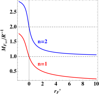
Figure 1: The generic profile of the variation of $M_{F_{(n)}}/R^{-1}$ as a function of $r^{\prime}_{F}\,(=r_{F}R^{-1})$ for the cases $n=1$ and $n=2$.

On the other hand, vanishing KK masses at level ‘0’ are always realized for $\phi^{+}$ and $\chi$ which are eventually “eaten up” by the massless level ‘0’ $W_{\mu}^{+},\,Z_{\mu}$ states respectively as they become massive. However, no zero mode appears for $W_{y}^{+},\,Z_{y}$ since they are projected out by the $Z_{2}$-odd condition. The mode functions for the fields $W_{y}^{+},\,Z_{y}$ are given by

$$f_{F_{(n)}}(y) =N_{F_{(n)}}\times\begin{cases}\displaystyle\frac{\sin(M_{F_{(n)}}y)}{C_{F_{(n)}}}&\text{for even }n,\\ \displaystyle\frac{\cos(M_{F_{(n)}}y)}{S_{F_{(n)}}}&\text{for odd }n\\ \end{cases}$$ (13)

with the mass-determination condition as given in equation 8. Use of equation 47 allows one to eliminate $\chi$ in favor of $Z_{y}$ and $\phi^{+}$ in favor of $W_{y}^{+}$. Correct normalization of the kinetic terms requires $Z_{y}$ and $W_{y}^{+}$ to be renormalized in the following way:

$$Z_{y}^{(n)}\to\left(1+\frac{M_{{Z_{y}}_{(n)}}^{2}}{M_{Z}^{2}}\right)^{-1/2}Z_{y}^{(n)}\,,\qquad\qquad W_{y}^{{(n)}{+}}\to\left(1+\frac{M_{{W_{y}}_{(n)}}^{2}}{M_{W}^{2}}\right)^{-1/2}W_{y}^{{(n)}{+}}.$$ (14)

Note that $Z_{y}^{(n)}$ is the pseudoscalar Higgs state and $W_{y}^{{(n)}{+}}$ is the charged Higgs boson from the $n$-th KK level which has no level ‘0’ counterpart. In subsequent phenomenological discussions we use the more transparent notations $A^{(n)^{0}}$ and $H^{(n)^{+}}$ for ${Z_{y}}^{(n)}$ and $W_{y}^{{(n)}{+}}$, respectively. Thus, up to KK level ‘1’, the Higgs spectrum consists of the following five Higgs bosons: the SM (level ‘0’) Higgs boson ($H$) and four Higgs states from level ‘1’, i.e., the neutral $CP$-even Higgs boson ($H^{(1)^{0}}$) which is the level ‘1’ excitation of the SM Higgs boson, the neutral $CP$-odd Higgs boson ($A^{(1)^{0}}$) and the two charged Higgs bosons $H^{(1)^{\pm}}$. For the rest of the paper, we use a modified convention for the (KK) gluon to be $g^{(n)}$ instead of $G^{(n)}$ for convenience.

2.2 The top quark sector

We start with the following general framework for the fermion sector where, in addition to fermion BLKTs, we incorporate brane-local Yukawa terms (BLYTs):

$$S_{\text{quark}} =\int d^{4}x\int_{-L}^{L}dy\sum_{i=1}^{3}\Bigg{\{}+i\overline{U^{\prime}_{i}}\Gamma^{M}\mathcal{D}_{M}U^{\prime}_{i}+r_{U_{i}}\Big{(}\delta(y-L)+\delta(y+L)\Big{)}\Big{[}i\overline{U^{\prime}_{i}}\Gamma^{\mu}\mathcal{D}_{\mu}P_{L}U^{\prime}_{i}\Big{]}$$

$$\phantom{=\int d^{4}x\int_{-L}^{L}dy\sum_{i=1}^{3}\Bigg{\{}\,\,}+i\overline{D^{\prime}_{i}}\Gamma^{M}\mathcal{D}_{M}D^{\prime}_{i}+r_{D_{i}}\Big{(}\delta(y-L)+\delta(y+L)\Big{)}\Big{[}i\overline{D^{\prime}_{i}}\Gamma^{\mu}\mathcal{D}_{\mu}P_{L}D^{\prime}_{i}\Big{]}$$

$$\phantom{=\int d^{4}x\int_{-L}^{L}dy\sum_{i=1}^{3}\Bigg{\{}\,\,}+i\overline{u^{\prime}_{i}}\Gamma^{M}\mathcal{D}_{M}u^{\prime}_{i}+r_{u_{i}}\Big{(}\delta(y-L)+\delta(y+L)\Big{)}\Big{[}i\overline{u^{\prime}_{i}}\Gamma^{\mu}\mathcal{D}_{\mu}P_{R}u^{\prime}_{i}\Big{]}$$

$$\phantom{=\int d^{4}x\int_{-L}^{L}dy\sum_{i=1}^{3}\Bigg{\{}\,\,}+i\overline{d^{\prime}_{i}}\Gamma^{M}\mathcal{D}_{M}d^{\prime}_{i}+r_{d_{i}}\Big{(}\delta(y-L)+\delta(y+L)\Big{)}\Big{[}i\overline{d^{\prime}_{i}}\Gamma^{\mu}\mathcal{D}_{\mu}P_{R}d^{\prime}_{i}\Big{]}\Bigg{\}},$$ (15)

$$S_{\text{Yukawa}} =\int d^{4}x\int_{-L}^{L}dy\sum_{i,j=1}^{3}\Bigg{\{}-\Big{(}1+r_{Y}(\delta(y-L)+\delta(y+L))\Big{)}\Big{[}\hat{Y}^{u}_{ij}\overline{Q^{\prime}_{i}}u^{\prime}_{j}\tilde{\Phi}+\hat{Y}^{d}_{ij}\overline{Q^{\prime}_{i}}d^{\prime}_{j}\Phi+\text{h.c.}\Big{]}\Bigg{\}},$$ (16)

where $U^{\prime}_{i},D^{\prime}_{i},u^{\prime}_{i},d^{\prime}_{i}$ correspond to the 5D $SU(2)_{W}$ up-doublet, down-doublet, up-singlet and down-singlet of the $i$-th generation, respectively and $Q^{\prime}_{i}\,\equiv\,(U^{\prime}_{i},D^{\prime}_{i})^{\text{T}}$ is the compact notation used for the $i$-th 5D doublet. $r_{U_{i}}$ and $r_{u_{i}}$ are the coefficients of the corresponding BLKTs. The field $\Phi$ represents the 5D Higgs scalar with $\tilde{\Phi}\,\equiv\,i\sigma_{2}\Phi^{\ast}$, $\sigma_{2}$ being the second Pauli matrix. $r_{Y}$ is the universal coefficient for the brane-local Yukawa term. We adopt the 5D Minkowski metric to be $\eta_{MN}=\text{diag}(1,-1,-1,-1,-1)$ and the representation of the Clifford algebra is chosen to be $\Gamma^{M}=\{\gamma^{\mu},i\gamma_{5}\}$. The 4D chiral projectors for (4D) right/left-handed states are defined following the standard convention i.e., $P_{R\atop L}=(1\pm\gamma_{5})/2$. $\mathcal{D}_{M}$ stands for the 5D covariant derivative.

In the presence of non-vanishing BLKT in the gauge sector (see equation 2), the 5D VEV of $\Phi$ is given by

$$\langle\Phi\rangle=\begin{pmatrix}0\\ \frac{\hat{v}}{\sqrt{2}}\end{pmatrix}=\begin{pmatrix}0\\ \frac{v}{\sqrt{2}}\frac{1}{\sqrt{\pi R+2r_{\text{EW}}}}\end{pmatrix}$$ (17)

where $v=246$ GeV is the usual 4D Higgs VEV associated with the breaking of electroweak symmetry. The 5D Yukawa couplings $\hat{Y}^{u}_{ij},\hat{Y}^{d}_{ij}$ are related to their 4D counterparts ${Y}^{u}_{ij},{Y}^{d}_{ij}$ as

$${Y}^{u/d}_{ij}=\frac{\hat{Y}^{u/d}_{ij}}{\sqrt{\pi R+2r_{\text{EW}}}}.$$ (18)

The free part of $S_{\text{quark}}$ has already been discussed in Datta:2012tv and hence we skip the details. Using that we can KK-expand the mass terms in $S_{\text{Yukawa}}$ as follows:

$$-\int d^{4}x\sum_{i,j=1}^{3}\frac{v}{\sqrt{2}}\bigg{\{}Y^{u}_{ij}F^{u,(0,0)}_{ij}\overline{u^{\prime(0)}_{iL}}u^{\prime(0)}_{jR}+Y^{d}_{ij}F^{d,(0,0)}_{ij}\overline{d^{\prime(0)}_{iL}}d^{\prime(0)}_{jR}+\text{h.c.}\bigg{\}},$$ (19)

where, for simplicity, we only present the zero-mode part with fields redefined (to make them appear more conventional) as $u^{\prime(0)}_{iL}\,\equiv\,U^{\prime(0)}_{iL}$, $d^{\prime(0)}_{iL}\,\equiv\,D^{\prime(0)}_{iL}$. The fermionic mode functions for KK decomposition are described in an appropriate context in section 3. The concrete forms of the factors $F^{u/d,(0,0)}_{ij}$ (which arise from the mode functions of the $L$, $R$ type fields participating in equation 19) are

$$F^{u,(0,0)}_{ij}=\frac{2r_{Y}+\pi R}{\sqrt{2r_{U_{i}}+\pi R}\sqrt{2r_{u_{i}}+\pi R}},\quad F^{d,(0,0)}_{ij}=\frac{2r_{Y}+\pi R}{\sqrt{2r_{D_{i}}+\pi R}\sqrt{2r_{d_{i}}+\pi R}}.$$ (20)

The $3\times 3$ matrices $Y^{u}_{ij}F^{u,(0,0)}_{ij}$ and $Y^{d}_{ij}F^{d,(0,0)}_{ij}$ are diagonalized by the following bi-unitary transformations

$$q^{\prime(0)}_{iR}=(U_{qR})_{ij}q^{(0)}_{jR},\quad q^{\prime(0)}_{iL}=(U_{qL})_{ij}q^{(0)}_{jL}\qquad(\text{for}\ q=u,d),$$ (21)

as follows:

$$-\int d^{4}x\sum_{i=1}^{3}\frac{v}{\sqrt{2}}\bigg{\{}\mathcal{Y}^{u}_{ii}\overline{u^{(0)}_{iL}}u^{(0)}_{iR}+\mathcal{Y}^{d}_{ii}\overline{d^{(0)}_{iL}}d^{(0)}_{iR}+\text{h.c.}\;\text{(+ KK excitations)}\bigg{\}},$$ (22)

where $\mathcal{Y}^{u}_{ii}$ and $\mathcal{Y}^{d}_{ii}$ are the diagonalized Yukawa couplings for up and down quarks, respectively. We discuss later in this paper that the diagonalized values do not directly correspond to those in the SM due to level mixing effects. Also, from now on, we would consider universal values of the BLKT parameters $r_{Q}$ for the quarks from the first two generations and $r_{T}$ for those from the third generation replacing the many different ones appearing in equation 15. We will see later, this provides us with a separate handle (modulo some constraints from experiments) on the top quark sector of the nmUED scenario under consideration. Further, this simplifies the expressions in equation 20.

3 Mixings, masses and effective couplings

Mixings in the fermion sector, quite generically, could have interesting implications as these affect both couplings and the spectra of the concerned excitations. Fermions with a certain flavor from a given KK level and belonging to $SU(2)_{W}$ doublet and singlet representations always mix once the electroweak symmetry is broken. Presence of BLTs affects such a mixing at every KK level. On top of this, the dynamics driven by the BLTs allows for mixing of fermions from different KK levels that have the same KK-parity. Both kinds of mixings are proportional to the Yukawa mass of the fermion in reference and thus, are pronounced for the top quark sector.

As pointed out in the introduction, since level-mixing among the even KK-parity top quarks involves the SM top quark (from level ‘0’), this naturally evokes a reasonable curiosity about its consequences and it is indeed found to give rise to interesting phenomenological possibilities. However, the phenomenon draws significant constraints from experiments which we will discuss in some detail. We restrict ourselves to the mixing of level ‘0’-level ’2’ KK top quarks ignoring all higher even KK states the effects of which would be suppressed by their increasing masses. Also, we do not consider the effects of level-mixings among KK states from levels with $n>0$, including say, those among the excitations from levels with odd KK-parity. Generally, these could be appreciable. However, in contrast to the case where SM excitations mix with higher KK levels, these would only entail details within a sector yet to be discovered.

3.1 Mixing in level ‘1’ top quark sector

We first briefly recount Datta:2012tv the mixing of the top quarks at KK level ‘1’. In presence of BLTs, the Yukawa part of the action embodying the mass-matrix is of the form

$$-\int d^{4}x\Bigg{\{}\begin{bmatrix}\overline{T}^{(1)},\ \overline{t}^{(1)}\end{bmatrix}_{L}\begin{bmatrix}M_{T_{(1)}}&r^{\prime}_{T11}m_{t}^{\text{in}}\\ -R^{\prime}_{T11}m_{t}^{\text{in}}&M_{T_{(1)}}\end{bmatrix}\begin{bmatrix}T^{(1)}\\ t^{(1)}\end{bmatrix}_{R}+\text{h.c.}\Bigg{\}},$$ (23)

with “input” top mass $m_{t}^{\text{in}}$ (which is an additional free parameter in our scenario) and

$$r^{\prime}_{T11} =\frac{1}{R_{T00}}\int_{-L}^{L}dy\Big{(}1+r_{Y}\left(\delta(y-L)+\delta(y+L)\right)\Big{)}f_{T_{(1)}}^{2}$$

$$=\frac{2r_{T}+\pi R}{2r_{Y}+\pi R}\times\frac{2r_{Y}+\frac{1}{S_{T_{(1)}}^{2}}\left[\frac{\pi R}{2}-\frac{1}{2M_{T_{(1)}}}\sin(M_{T_{(1)}}\pi R)\right]}{2r_{T}+\frac{1}{S_{T_{(1)}}^{2}}\left[\frac{\pi R}{2}-\frac{1}{2M_{T_{(1)}}}\sin(M_{T_{(1)}}\pi R)\right]},$$ (24)

$$R^{\prime}_{T11} =\frac{1}{R_{T00}}\int_{-L}^{L}dy\Big{(}1+r_{Y}\left(\delta(y-L)+\delta(y+L)\right)\Big{)}g_{T_{(1)}}^{2}$$

$$=\frac{2r_{T}+\pi R}{2r_{Y}+\pi R}\times\frac{2r_{Y}(C_{T_{(1)}}/S_{T_{(1)}})^{2}+\frac{1}{S_{T_{(1)}}^{2}}\left[\frac{\pi R}{2}+\frac{1}{2M_{T_{(1)}}}\sin(M_{T_{(1)}}\pi R)\right]}{\frac{1}{S_{T_{(1)}}^{2}}\left[\frac{\pi R}{2}+\frac{1}{2M_{T_{(1)}}}\sin(M_{T_{(1)}}\pi R)\right]}$$ (25)

where $R_{T00}$ is given by

$$R_{T00} =\int_{-L}^{L}dy\Big{(}1+r_{Y}\left(\delta(y-L)+\delta(y+L)\right)\Big{)}f_{T_{(0)}}^{2}=\frac{2r_{Y}+\pi R}{2r_{T}+\pi R}.$$ (26)

$f_{T_{(n)}}$ and $g_{{}_{T_{(n)}}}$ represent the mode functions for $n$-th KK level and are given by Datta:2012tv :

$$f_{T_{(n)}}\;\equiv\;f_{T_{(n)L}}=f_{t_{(n)R}} =N_{T_{(n)}}\times\begin{cases}\displaystyle\frac{\cos(M_{T_{(n)}}y)}{C_{T_{(n)}}}&\text{for $n$ even,}\\ \displaystyle\frac{{-}\sin(M_{T_{(n)}}y)}{S_{T_{(n)}}}&\text{for $n$ odd,}\end{cases}$$ (27)

$$g_{{}_{T_{(n)}}}\;\equiv\;f_{T_{(n)R}}=-f_{t_{(n)L}} =N_{T_{(n)}}\times\begin{cases}\displaystyle\frac{\sin(M_{T_{(n)}}y)}{C_{T_{(n)}}}&\text{for $n$ even,}\\ \displaystyle\frac{\cos(M_{T_{(n)}}y)}{S_{T_{(n)}}}&\text{for $n$ odd}\end{cases}$$ (28)

with

$$C_{T_{(n)}}=\cos\left(\frac{M_{T_{(n)}}\pi R}{2}\right),\quad S_{T_{(n)}}=\sin\left(\frac{M_{T_{(n)}}\pi R}{2}\right)$$ (29)

and the normalization factors $N_{T_{(n)}}$ for the mode functions are given by

$$N_{T_{(n)}}^{-2}=\begin{cases}\displaystyle 2r_{T}+\frac{1}{C_{T_{(n)}}^{2}}\left[\frac{\pi R}{2}+\frac{1}{2M_{T_{(n)}}}\sin(M_{T_{(n)}}\pi R)\right]&\text{for $n$ even,}\\ \displaystyle 2r_{T}+\frac{1}{S_{T_{(n)}}^{2}}\left[\frac{\pi R}{2}-\frac{1}{2M_{T_{(n)}}}\sin(M_{T_{(n)}}\pi R)\right]&\text{for $n$ odd.}\end{cases}$$ (30)

The KK mass $M_{T_{(n)}}$ for the ‘$n$’-th level top quark excitation follows from equation 12 where chiral zero modes occur. Note that the off-diagonal terms are asymmetric and pick up nontrivial multiplicative factors. This is because two different mode functions, $f_{T_{(n)}}$ and $g_{{}_{T_{(n)}}}$ (associated with the specific states with particular chiralities and gauge quantum numbers), contribute to them. On the other hand, the diagonal KK mass terms are now solutions of the appropriate transcendental equations. When expanded, the diagonal entries of the mixing matrix involve the $L$ and $R$ components of the same gauge multiplet ($T$ from $SU(2)_{W}$ doublet or $t$ from $SU(2)_{W}$ singlet). In contrast, the off-diagonal entries are of Yukawa-origin (signalled by the presence of $m_{t}^{\text{in}}$) and involve both $r_{T}$ and $r_{Y}$. These terms represent the conventional Dirac mass-terms as they connect the $L$ and the $R$ components belonging to two different multiplets. It may be noted that even when either $r_{T}$ or $r_{Y}$ vanishes, the mixing remains nontrivial. Only the case with $r_{T}$ $=$ $r_{Y}$ $=$ $0$ trivially reduces to the (tree-level) mUED.

The mass matrix of equation 23 can be diagonalized by bi-unitary transformation with the matrices $V_{tL}^{(1)}$ and $V_{tR}^{(1)}$ where

$$\begin{bmatrix}T^{(1)}\\ t^{(1)}\end{bmatrix}_{L}=V^{(1)}_{tL}\begin{bmatrix}t^{(1)}_{l}\\ t^{(1)}_{h}\end{bmatrix}_{L},\quad\begin{bmatrix}T^{(1)}\\ t^{(1)}\end{bmatrix}_{R}=V^{(1)}_{tR}\begin{bmatrix}t^{(1)}_{l}\\ t^{(1)}_{h}\end{bmatrix}_{R}.$$ (31)

Then, equation 23 takes the diagonal form

$$-\int d^{4}x\begin{bmatrix}\overline{t}^{(1)}_{l},\ \overline{t}^{(1)}_{h}\end{bmatrix}\begin{bmatrix}m_{t^{(1)}_{l}}&\\ &m_{t^{(1)}_{h}}\end{bmatrix}\begin{bmatrix}t^{(1)}_{l}\\ t^{(1)}_{h}\end{bmatrix}$$ (32)

where $t^{(1)}_{l},\;t^{(1)}_{h}$ are the level ‘1’ top quark mass eigenstates and $(m_{t^{(1)}_{l}})^{2}$ and $(m_{t^{(1)}_{l}})^{2}$ are the mass-eigenvalues of the squared mass-matrix with $m_{t^{(1)}_{h}}>m_{t^{(1)}_{l}}$. Note that, for clarity and convenience, we have modified the notations and the ordering of the states in the presentations above from what appear in ref. Datta:2012tv .

3.2 Mixing among level ‘0’ and level ‘2’ top quark states

The formulation described above can be extended in a straight-forward manner for the level ‘2’ KK top quarks when this sector is augmented by the level ‘0’ (SM) top quark. Thus, the mass-matrix for the even KK parity top quark sector (keeping only level ‘0’ and level ‘2’ KK excitations) takes the following form:

$$-\int d^{4}x\Bigg{\{}\begin{bmatrix}\overline{t^{(0)}},\ \overline{T}^{(2)},\ \overline{t}^{(2)}\end{bmatrix}_{L}\begin{bmatrix}m_{t}^{\text{in}}&0&m_{t}^{\text{in}}R^{\prime}_{T02}\\ m_{t}^{\text{in}}R^{\prime}_{T02}&M_{T_{(2)}}&m_{t}^{\text{in}}r^{\prime}_{T22}\\ 0&-m_{t}^{\text{in}}R^{\prime}_{T22}&M_{T_{(2)}}\end{bmatrix}\begin{bmatrix}t^{(0)}\\ T^{(2)}\\ t^{(2)}\end{bmatrix}_{R}+\text{h.c.}\Bigg{\}}$$ (33)

where $r^{\prime}_{T22}$, $R^{\prime}_{T22}$, $R^{\prime}_{T02}$ are defined as follows, in a way similar to the case for level ‘1’ top quarks:

$$r^{\prime}_{T22} =\frac{1}{R_{T00}}\int_{-L}^{L}dy\Big{(}1+r_{Y}\left(\delta(y-L)+\delta(y+L)\right)\Big{)}f_{T_{(2)}}^{2}$$

$$=\frac{2r_{T}+\pi R}{2r_{Y}+\pi R}\times\frac{2r_{Y}+\frac{1}{C_{T_{(2)}}^{2}}\left[\frac{\pi R}{2}+\frac{1}{2M_{T_{(2)}}}\sin(M_{T_{(2)}}\pi R)\right]}{2r_{T}+\frac{1}{C_{T_{(2)}}^{2}}\left[\frac{\pi R}{2}+\frac{1}{2M_{T_{(2)}}}\sin(M_{T_{(2)}}\pi R)\right]},$$ (34)

$$R^{\prime}_{T22} =\frac{1}{R_{T00}}\int_{-L}^{L}dy\Big{(}1+r_{Y}\left(\delta(y-L)+\delta(y+L)\right)\Big{)}g_{T_{(2)}}^{2}$$

$$=\frac{2r_{T}+\pi R}{2r_{Y}+\pi R}\times\frac{2r_{Y}(S_{T_{(2)}}/C_{T_{(2)}})^{2}+\frac{1}{C_{T_{(2)}}^{2}}\left[\frac{\pi R}{2}-\frac{1}{2M_{T_{(2)}}}\sin(M_{T_{(2)}}\pi R)\right]}{\frac{1}{C_{T_{(2)}}^{2}}\left[\frac{\pi R}{2}-\frac{1}{2M_{T_{(2)}}}\sin(M_{T_{(2)}}\pi R)\right]},$$ (35)

$$R^{\prime}_{T02} =\frac{1}{R_{T00}}\int_{-L}^{L}dy\Big{(}1+r_{Y}\left(\delta(y-L)+\delta(y+L)\right)\Big{)}f_{T_{(0)}}f_{T_{(2)}}$$

$$=\frac{2r_{T}+\pi R}{2r_{Y}+\pi R}\times\frac{2r_{Y}+2(S_{T_{(2)}}/M_{T_{(2)}}C_{T_{(2)}})}{\sqrt{2r_{T}+\pi R}\sqrt{2r_{T}+\frac{1}{C_{T_{(2)}}^{2}}\left[\frac{\pi R}{2}+\frac{1}{2M_{T_{(2)}}}\sin(M_{T_{(2)}}\pi R)\right]}},$$ (36)

with $R_{T00}$ given by equation 26. The lower $2\times 2$ block of the mass-matrix in equation 33 is reminiscent of the level ‘1’ top quark mass-matrix of equation 23. Beyond this, the mass-matrix contains as the first diagonal element the ‘input’ top quark mass, $m_{t}^{\text{in}}$ and two other non-vanishing off-diagonal elements as the 13 and 21 elements. Obviously, the latter two play direct roles in the mixings of the level ‘0’ and level ‘2’ top quarks. Note that all the off-diagonal terms of the mass-matrix are proportional to $m_{t}^{\text{in}}$ which is clearly indicative of their origins in the Yukawa sector. The zeros in turn reflect $SU(2)_{W}$ invariance.

Diagonalization of this $3\times 3$ mass-matrix yields the physical states (3 of them) along with their mass-eigenvalues. Thus, the level ‘0’ top quark (i.e., the SM top quark) ceases to be a physical state and mixes with the level ‘2’ top states. Given the rather involved structure of the mass-matrix, neither is it possible to express the eigenvalues analytically in a compact way nor they would be much illuminating theoretically. We, thus, diagonalize the mass-matrix numerically. Similar to the case of the level ‘1’ states, we adopt the following conventions:

$$\begin{bmatrix}t^{(0)}\\ T^{(2)}\\ t^{(2)}\end{bmatrix}_{L}=V_{tL}^{(2)}\begin{bmatrix}t\\ t^{(2)}_{l}\\ t^{(2)}_{h}\end{bmatrix}_{L},\quad\begin{bmatrix}t^{(0)}\\ T^{(2)}\\ t^{(2)}\end{bmatrix}_{R}=V_{tR}^{(2)}\begin{bmatrix}t\\ t^{(2)}_{l}\\ t^{(2)}_{h}\end{bmatrix}_{R}$$ (37)

with the physical masses $m_{t}^{\text{phys}}$, $m_{t^{(2)}_{l}}$ and $m_{t^{(2)}_{h}}$ and with the ordering $m_{t}^{\text{phys}}<m_{t^{(2)}_{l}}<m_{t^{(2)}_{h}}$.

3.3 Quantitative estimates

As can be seen from the equations above, the free parameters of the top-quark sector in the nmUED scenario under consideration are $R$, $r_{T}$ and $r_{Y}$. For the latter two, we use Datta:2012tv the dimensionless quantities $r_{T}^{\prime}$ and $r_{Y}^{\prime}$ where $r_{T}^{\prime}=r_{T}R{{}^{-1}}$ and $r_{Y}^{\prime}=r_{Y}R{{}^{-1}}$. In addition, $m_{t}^{\text{in}}$ serves as an extra free parameter from the SM sector.

3.3.1 Top quark masses

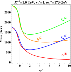
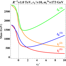
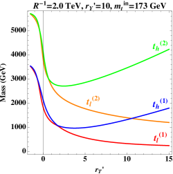
Figure 2: Masses of level ‘1’ and level ‘2’ KK top quarks as functions of $r_{T}^{\prime}$ for given $r_{Y}^{\prime}$ and $R{{}^{-1}}$ with $m_{t}^{\text{in}}=173\,\text{GeV}$.

In figure 2 we illustrate the variations of the masses, as functions of $r_{T}^{\prime}$, of the two KK top quark eigenstates from level ‘1’ and the two heavier mass eigenstates that result from the mixing of level ‘0’ and level ‘2’. The plot in the middle, when compared to the one in the left, demonstrates how the spectrum changes as $r_{Y}^{\prime}$ varies with $R{{}^{-1}}$ held fixed. We set the input top mass $m_{t}^{\text{in}}$ to $173\,\text{GeV}$ in all the plots of figure 2. In turn, the effect of changing $R{{}^{-1}}$ can be seen as one goes from the plot in the middle ($R{{}^{-1}}=1$ TeV) to the one on the right ($R{{}^{-1}}=2$ TeV). An interesting feature common to all these plots is that there is a cross-over of the curves for $m_{t^{(1)}_{h}}$ and $m_{t^{(2)}_{l}}$, i.e., as a function of $r_{T}^{\prime}$, at some point, the lighter of the mixed level ‘2’ state top quark eigenstates becomes less massive compared to the heavier of the level ‘1’ KK top quark eigenstate. The cross-overs take place at smaller values of $r_{T}^{\prime}$ when $r_{Y}^{\prime}$ is increased for a given $R{{}^{-1}}$ and at larger values of $r_{T}^{\prime}$ when $R{{}^{-1}}$ is increased with $r_{Y}^{\prime}$ held fixed. Accordingly, the mass-values at those flipping points also go down or up, respectively. Here, the dominant role is being played by the ‘chiral mixing’ while level-mixing is unlikely to have much bearing. These plots also reveal that achieving a ‘flipped-spectrum’ (in the above sense) is difficult if one requires the light level ‘1’ KK top quark to be heavier than about 400 GeV. Nonetheless, the overall trend could provide easier reach for a KK top quark from level ‘2’ at the LHC. Thus, it may be possible for up to three excited top quark states ($m_{t^{(1)}_{l}},\,m_{t^{(1)}_{h}},\,m_{t^{(2)}_{l}}$) to pop up at the LHC.

3.3.2 Top quark mixings

In this subsection we take a quantitative look at the mixings in the top quark sector from the first KK level discussed earlier in section 3.1. The mixing is known to be near-maximal in the case of quarks (fermions) from the lighter generations Datta:2012tv . Deviations from such maximal mixings occur in the top quark sector due to its nontrivial structure. Such mixings are expected to follow similar trends at level ‘2’ (and higher) KK levels and hence we do not present them separately. However, some deviations are expected in the presence of level-mixings which can at best be modest for the case of $t^{(0)}-t^{(2)}$ system that we focus on in this work.

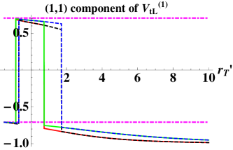
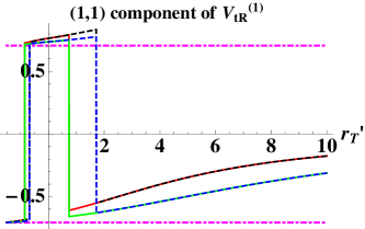
Figure 3: Variations of the (1,1) elements of the matrices $V^{(1)}_{tL}$ (left) and $V^{(1)}_{tL}$ (right) as functions of $r_{T}^{\prime}$ for fixed set of values of $R{{}^{-1}}$ and $r_{Y}^{\prime}$. Conventions used for different sets of $R{{}^{-1}}$ and $r_{Y}^{\prime}$ values are: bold red for $R{{}^{-1}}=1$ TeV and $r_{Y}^{\prime}=1$, dashed black for $R{{}^{-1}}=1$ TeV and $r_{Y}^{\prime}=10$, bold green for $R{{}^{-1}}=2$ TeV and $r_{Y}^{\prime}=1$ and dashed blue for $R{{}^{-1}}=2$ TeV and $r_{Y}^{\prime}=10$.

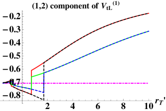
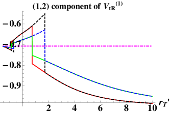
Figure 4: Same as in figure 3 but for the variations of the (1,2) elements of the matrices $V^{(1)}_{tL}$ (left) and $V^{(1)}_{tL}$ (right). The respective (2,1) elements can be obtained from the orthogonality of these matrices.

The elements of the $V$-matrices in equation 31 give the admixtures of different participating states in the KK top quark eigenstates. To be precise, $V^{(1)}_{{tL}_{(1,1)}}$ and $V^{(1)}_{{tL}_{(2,2)}}$ represent the admixture of $T_{L}^{(1)}$ in $t^{(1)}_{lL}$ and $t_{L}^{(1)}$ in $t^{(1)}_{hL}$ respectively while $V^{(1)}_{{tL}_{(1,2)}}$ and $V^{(1)}_{{tL}_{(2,1)}}$ indicate the same for $t_{L}^{(1)}$ in $t^{(1)}_{lL}$ and $T_{L}^{(1)}$ in $t^{(1)}_{hL}$ in that order. Similar descriptions hold for the $V_{R}^{(1)}$ matrix. In figures 3 and 4 we illustrate the deviations from maximal mixing in the level ‘1’ top quark sector in terms of these components of the $V$ matrices as functions of $r_{T}^{\prime}$. Each figure contains multiples curves which present situations for different combinations of $R{{}^{-1}}$ and $r_{Y}^{\prime}$ (see the captions for details). Note that the abrupt changes in sign of the mixings that happen between $-1<r_{T}^{\prime}<2$ can be understood in terms of the trends of the red and blue curves in figure 2 (the blue curves smoothly evolve to the red ones and vice-versa).

The flat, broken magenta lines indicate maximal mixing ($|V^{(1)}_{{tL}_{(1,1)}}|=|V^{(1)}_{{tL}_{(1,2)}}|=1/\sqrt{2}$). It is clear from these figures that there can be appreciable deviations from maximal mixing in all these cases. As can be seen, the effects are bigger for larger values of $r_{T}^{\prime}$ and smaller $R{{}^{-1}}$. Some dependence on $r_{Y}^{\prime}$ is observed for smaller values of $r_{T}^{\prime}$. However, it is to be kept in mind that the effective deviations arise from the interplay of these elements which is again neither easy to present nor much illuminating.

3.4 Effective couplings

As mentioned earlier, not only masses undergo modifications in the presence of BLTs but also the wavefunctions get distorted. The latter affects the couplings through the overlap integrals. These are integrals over the extra dimension of a product of mode functions of the states that appear at a given interaction vertex. In this section we briefly discuss the generic properties of some of these overlap integrals which play roles in the present study. Assuming the wavefunctions to be real, the general form of the multiplicative factor that scales the corresponding SM coupling strengths is given by

$$g_{f_{i}^{(l)}f_{j}^{(m)}f_{k}^{(n)}}=\mathcal{N}_{ijk}\int_{-L}^{L}dy\Big{[}1+r_{ijk}^{(l,m,n)}\left(\delta(y-L)+\delta(y+L)\right)\Big{]}f_{i}^{(l)}(y)f_{j}^{(m)}(y)f_{k}^{(n)}(y)$$ (38)

where $i,j,k$ represent different interacting fields and $f_{i}^{(l)},f_{j}^{(m)},f_{k}^{(n)}$ are the corresponding mode functions with the KK indices $l,m,n$, respectively, as defined in sections 2.1, 3.1 and 3.2. The factor $r_{ijk}^{(l,m,n)}$ stands for relevant BLT parameter(s) while the normalization factor $\mathcal{N}_{ijk}$ is suitably chosen to recover the SM vertices when $l$=$m$=$n$=0 (except for the Yukawa sector of the nmUED scenario under consideration).

The key to understand the general structure is the flatness of the zero-mode ($n=0$) profiles in our minimal configuration. For these, the factor takes the following form:

$$g_{f_{i}^{(l)}f_{j}^{(m)}f_{k}^{(0)}}=\mathcal{N}_{ijk}f_{k}^{(0)}\int_{-L}^{L}dy\Big{[}1+r_{ijk}^{(l,m,0)}\left(\delta(y-L)+\delta(y+L)\right)\Big{]}f_{i}^{(l)}(y)f_{j}^{(m)}(y),$$ (39)

where we see the zero-mode field has been taken out of the integral in equation 38. For $i=j$, the overlap integral reduces to Kronecker’s delta function, $\delta_{l,m}$ and the overall strength turns out to be identically equal to 1. Orthonormality of the involved states constrains the possibilities. In table 1 we collect some of these interactions and group them in terms of their effective strengths (given by equation 39). This list, in particular, the set of couplings in the third column, is not exhaustive and presented for demonstrative purposes only.

In addition to these, mixings in the top quark sector in the form of both chiral mixing and level-mixing play roles in determining the effective couplings. In this subsection we briefly discuss such effects on some of the important interaction-vertices involving the top quarks, the gauge and the Higgs bosons from different KK levels. As in section 3.3, we further introduce the dimensionless parameters $r_{\text{EW}}^{\prime}\,(=R^{-1}r_{\text{EW}})$, $r_{Q}^{\prime}\,(=R^{-1}r_{Q})$ and $r_{G}^{\prime}\,(=R^{-1}r_{G})$ replacing $r_{\text{EW}}\,(=r_{H})$, $r_{Q}$ and $r_{G}$, the BLKT parameters for the electroweak gauge boson and Higgs sectors, the first two generation quark sector and the gluon sector, respectively. In addition, we also introduce a corresponding universal parameter $r_{L}$ for the lepton sector which we will use in section 4.3. Later, in section 5, we will refer back to this discussion in the context of phenomenological analyses of the scenario.

		$Q_{R/L}^{(1)}-{V}^{(1)}-Q_{R/L}^{(0)}$
	$V^{(2)}-V^{(2)}-V^{(0)}$	$q_{R/L}^{(1)}-{V}^{(1)}-q_{R/L}^{(0)}$
	$V^{(1)}-V^{(1)}-V^{(0)}$	$Q_{R/L}^{(0)}-{V}^{(2)}-Q_{R/L}^{(0)}$
	$Q_{R/L}^{(1)}-{V}^{(0)}-Q_{R/L}^{(1)}$	$Q_{L}^{(1)}-{H}^{(0)}-q_{R}^{(1)}$
$Q_{R/L}^{(2)}-{V}^{(0)}-Q_{R/L}^{(0)}$	$q_{R/L}^{(1)}-{V}^{(0)}-q_{R/L}^{(1)}$	$Q_{L}^{(2)}-{H}^{(0)}-q_{R}^{(0)}$
$q_{R/L}^{(2)}-{V}^{(0)}-q_{R/L}^{(0)}$	$Q_{R/L}^{(2)}-{V}^{(0)}-Q_{R/L}^{(2)}$	$Q_{L}^{(0)}-{H}^{(2)}-q_{R}^{(0)}$
${V}^{(2)}-{V}^{(0)}-{V}^{(0)}$	$q_{R/L}^{(2)}-{V}^{(0)}-q_{R/L}^{(2)}$	$Q_{L}^{(0)}-{H}^{(0)}-q_{R}^{(2)}$
0	1	non-zero

Table 1: Classes of different effective (tree level) couplings (given by equation 39) involving the gauge boson ($V$), Higgs ($H$) and the left- and right-handed, $SU(2)_{W}$ doublet ($Q$) and singlet ($q$) quark excitations and their relative strengths (shown in the last row) compared to the corresponding SM cases.

3.4.1 Effective couplings involving the gauge bosons

The set of couplings that we briefly discuss here are those that would appear in the production of the KK top quarks at the LHC and their decays. In figure 5 we illustrate the coupling-deviation (a multiplicative factor of the corresponding SM value at the tree level) $g^{(2)}$-$q^{(0)}$-$q^{(0)}$ (left) and $g^{(2)}$-$q^{(2)}$-$q^{(0)}$ (right) in the generic $r^{\prime}_{V}-r^{\prime}_{Q/T/L}$ plane. In both of these plots, the mUED case is realized along the diagonals over which $r_{G}^{\prime}=r_{Q}^{\prime}$. In the first case, the mUED value is known to be vanishing at the tree level since KK number is violated. Hence, the diagonal appears with the contour-value of zero. For vertices involving the top quarks, $r_{T}^{\prime}$ replaces $r_{Q}^{\prime}$. For a process like $pp\to\bar{t}^{(2)}_{l}t$ + h.c., the former kind of coupling appears at the parton-fusion (initial state) vertex while the latter shows up at the production vertex. The combined strength of these two couplings controls the production rate for the mentioned process. Further, the situation is not much different for the level ‘2’ electroweak gauge bosons except for some modifications due to mixings present in the electroweak sector. In general, it can be seen from the first plot of figure 5 that the coupling $g^{(2)}$-$q^{(0)}$-$q^{(0)}$ picks up a negative sign for $r_{G}^{\prime}>r_{Q}^{\prime}$. This could have nontrivial phenomenological implications for processes in which interfering Feynman diagrams are present. On the other hand, $g^{(2)}$-$q^{(2)}$-$q^{(0)}$ remains always positive as is clear from the second plot of figure 5. Note that the three-point vertex $V^{(0)}$-$V^{(0)}$-$V^{(2)}$ and the generic ones of the form $V^{(0)}$-$f^{(0)}$-$f^{(2)}$ are absent because the corresponding overlap integrals vanish due to orthogonality of the involved mode functions.

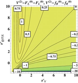
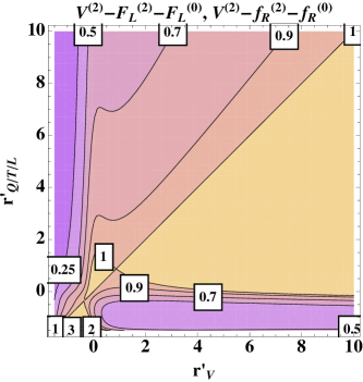
Figure 5: Contours of deviation for the generic couplings $V^{(2)}$-$F^{(0)}$-$F^{(0)}$ (or $V^{(2)}$-$f^{(0)}$-$f^{(0)}$) (left) and $V^{(2)}$-$F^{(2)}$-$F^{(0)}$ (or $V^{(2)}$-$f^{(2)}$-$f^{(0)}$) (right) from the corresponding SM values in the $r^{\prime}_{V}-r^{\prime}_{Q/T/L}$ plane. $V$, $F$ and $f$ stand for generic gauge boson, $SU(2)_{W}$ doublet and singlet fermion fields (with corresponding chiralities), respectively. Note that when $V$ is the (KK) $W$ boson, types of the two fermions involved at a given vertex are different.

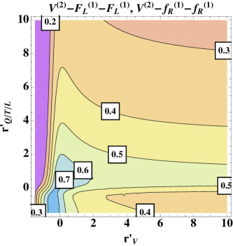
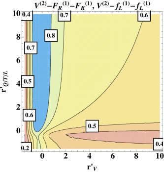
Figure 6: Same as in figure 5 but for the generic couplings $V^{(2)}$-$F^{(1)}_{L}$-$F^{(1)}_{L}$ or $V^{(2)}$-$f^{(1)}_{R}$-$f^{(1)}_{R}$ (left) and $V^{(2)}$-$f^{(1)}_{L}$-$f^{(1)}_{L}$ or $V^{(2)}$-$F^{(1)}_{R}$-$F^{(1)}_{R}$ (right).

In figure 6 we present the corresponding contours of similar deviations in the couplings involving the level ‘2’ KK gauge bosons and the level ‘1’ KK quarks. The plot on left shows the situation for the left- (right-) chiral component of the $SU(2)_{W}$ doublet (singlet) quarks while the plot on right illustrates the case for left- (right-) chiral component of the $SU(2)_{W}$ singlet (doublet) quarks. These are in conformity with the mode functions for these individual components of the level ‘1’ KK quarks. However, it should be noted that the KK quarks being vector-like states, each of the $SU(2)_{W}$ doublet and singlet partners have both left- and right-chiral components. Thus, the effective couplings are obtained only by suitably combining (with appropriate weights) the strengths as given by the two plots. In the case of KK top quarks, the situation would be further complicated because of significant mixing between the two gauge eigenstates. For brevity, a list of relevant couplings is presented in table 1 with mentions of the kind of modifications they undergo in the nmUED scenario. It is clear from these figures that these (component) couplings involving level ‘2’ KK states are in general suppressed compared to the relevant SM couplings except over a small region with $r^{\prime}_{Q/T/L}<0$.

3.4.2 Effective couplings involving the Higgs bosons

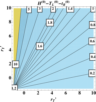
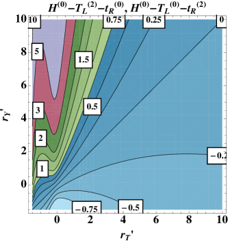
Figure 7: Contours of deviation in the $r_{T}^{\prime}-r_{Y}^{\prime}$ plane for the generic couplings $H^{(0)}$-$T^{(0)}_{L}$-$t^{(0)}_{R}$ (left) and $H^{(0)}$-$T^{(2)}_{L}$-$t^{(0)}_{R}$ or $H^{(0)}$-$T^{(0)}_{L}$-$t^{(2)}_{R}$ compared to the corresponding SM cases.

The association of the Higgs sector with the third SM family is rather intricate and has deep implications which unfold themselves in many scenarios beyond the SM. SUSY scenarios provide very good examples of this, some analyses have been done in the mUED Bandyopadhyay:2009gd and the nmUED scenario is also no exception. The couplings among the Higgs bosons and the KK top quarks of the nmUED scenario can deviate significantly from the corresponding SM Yukawa coupling. However, the zero-mode (SM) Higgs Yukawa couplings do not depend upon $r_{H}^{\prime}\,(=r_{\text{EW}}^{\prime})$. In the left panel of figure 7 we illustrate the possible deviation in the SM Yukawa coupling itself in the $r_{T}^{\prime}-r_{Y}^{\prime}$ plane. Along the diagonal of this figure (with $r_{T}^{\prime}=r_{Y}^{\prime}$) the SM value of the Yukawa coupling is preserved. Note that the latest LHC data still allows for significant deviations in the $H$-$t$-$t$ coupling Chatrchyan:2013yea ; cms-tth-gamma ; atlas-tth-gamma ; Nishiwaki:2013cma .

In the right panel we show deviations of the generic $H$-$t^{(2)}$-$t$ which appears at the tree level in nmUED. Unlike in the case of the interaction vertex $V^{(0)}$-$f^{(2)}$-$f^{(0)}$ (where $V^{(0)}$ is a massive SM gauge boson) where the involved coupling vanishes in the absence of level-mixing between $f^{(2)}$ and $f^{(0)}$, the analogous Higgs vertex remains non-vanishing even in the absence of level-mixing between the fermions. However, in this case, for $r_{T}^{\prime}=r_{Y}^{\prime}$ the coupling vanishes. This implies that the more the Yukawa coupling involving the level ‘0’ fields appears to agree with the SM expectation (from future experimental analyses), the weaker the coupling $H$-$t^{(2)}$-$t$ in such a scenario would get to be. In both cases, however, we find that the coupling strengths get enhanced for smaller values of $r_{T}^{\prime}$ with $r_{T}^{\prime}<r_{Y}^{\prime}$. All these indicate that production of the SM Higgs boson via gluon-fusion and its decay to di-photon final state can receive non-trivial contributions from such couplings and thus might get constrained from the LHC data. The issue is currently under study.

4 Experimental constraints and benchmark scenarios

Several different experimental observations put constraints of varying degrees on the parameters (like $R{{}^{-1}}$, $r_{T}^{\prime}$, $r_{Q}^{\prime}$, $r_{Y}^{\prime}$ and the input top quark mass ($m_{t}^{\text{in}}$)) that control the KK top quark sector. First and foremost, $R{{}^{-1}}$ is expected to be constrained from the searches for level ‘1’ KK quarks and KK gluon at the LHC. In the absence of any such dedicated search, a rough estimate of $R{{}^{-1}}>1$ TeV has been derived in ref. Datta:2012tv by appropriate recast of the LHC constraints obtained for the squarks and the gluino in SUSY scenarios.

As discussed in the previous subsection, observed mass of the top quark restricts the parameter space in a nontrivial way. Also, important constraints come from the experimental bounds on flavor changing neutral currents (FCNC), electroweak precision bounds in terms of the Peskin–Takeuchi parameters ($S,\,T$ and $U$) and bounds on effective four-fermion interactions. In this section we discuss these constraints briefly and choose a few benchmark scenarios that satisfy them and are phenomenologically interesting.

4.1 Constraints from the observed mass of the SM-like top quark

In figure 8 we show the allowed regions in the $r_{T}^{\prime}-r_{Y}^{\prime}$ plane that result in top quark pole mass within the range 171-175 GeV Alekhin:2012py (which is argued to be a more appropriate range than what the experiments actually quote CDF:2013jga ) for given values of $R{{}^{-1}}$ and input top quark masses.

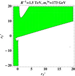
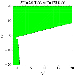
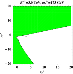
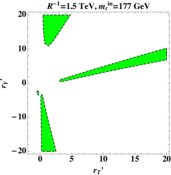
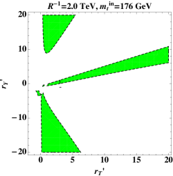
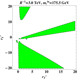
Figure 8: Regions (in green) in the $r_{T}^{\prime}-r_{Y}^{\prime}$ plane for three $R{{}^{-1}}$ values of (1.5, 2 and 3 TeV, varying along the rows) and for different suitable values of $m_{t}^{\text{in}}$ (indicated on top of each plot) that are consistent with physical (SM-like) top quark mass ($m_{t}^{\text{phys}}$) being within the range $m_{t}^{\text{phys}}=173\pm 2$ GeV.

Some general observations are that the physical top quark mass ($m_{t}^{\text{phys}}$) rarely becomes larger than the input top quark mass ($m_{t}^{\text{in}}$). This means, to have $m_{t}^{\text{phys}}$ at least of 171 GeV, $m_{t}^{\text{in}}$ has to be larger than 171 GeV. Further, increasing $m_{t}^{\text{in}}$ beyond around 175 GeV, as we go over to the second row of figure 8, opens up disjoint sets of allowed islands in the $r_{T}^{\prime}-r_{Y}^{\prime}$ plane with increasing region allowed for negative $r_{Y}^{\prime}$ (and extending to larger $r_{T}^{\prime}$ values) at the expense of the same with positive $r_{Y}^{\prime}$. Increasing $m_{t}^{\text{in}}$ further (beyond say, 180 GeV) results in allowed regions diminishing to an insignificant level. These features remain more or less unaltered as $R{{}^{-1}}$ is increased, as we go from left to right along a horizontal panel. A palpable direct effect that can be attributed to increasing $R{{}^{-1}}$ is in the moderate increase of the region in the $r_{T}^{\prime}-r_{Y}^{\prime}$ plane consistent with $m_{t}^{\text{phys}}$, in particular, for negative $r_{Y}^{\prime}$ values and when $m_{t}^{\text{in}}$ is not terminally large (i.e., below $190$ GeV, say) for the purpose.

Although a moderate range of input top quark mass $171<m_{t}^{\text{in}}\lesssim 190$ is consistent with $171<m_{t}^{\text{phys}}<175$ GeV in the space of $R{{}^{-1}}-r_{T}^{\prime}-r_{Y}^{\prime}$, the allowed region there is rather sensitive to the variation in $m_{t}^{\text{in}}$. Thus, the allowed range of the $m_{t}^{\text{phys}}$ restricts the nmUED parameter space in a significant way which, in turn, influences the masses and the couplings of the KK top quarks. An important point is to be noted here. The level ‘1’ top quark sector, though does not talk to either level ‘0’ or level ‘2’ sector directly (because of conserved KK-parity), is influenced by these constraints since $r_{T}^{\prime}$, $r_{Y}^{\prime}$ and $R{{}^{-1}}$ also govern the same.

4.2 Flavor constraints

The BLKTs ($r_{Q}^{\prime}$) and the BLYTs ($r_{Y}^{\prime}$) are matrices in the flavor space. Hence, their generic choices may induce large FCNCs at the tree level. It is possible to choose a basis in which the BLKT matrix is diagonal. This ensures no mixing among fermions of different flavors or from different KK levels arising from the gauge kinetic terms. However, with the Yukawa sector included, off-diagonal terms (mixings) appear in the gauge sector on rotating the gauge kinetic terms into a basis where the quark mass matrices are diagonal. These terms could induce unacceptable FCNCs at the tree levels and thus, would be constrained by experiments. In figure 9 we present the tree level diagram that could give rise to unwanted FCNC effects.

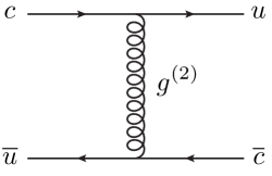
Figure 9: Feynman diagram showing the induced FCNC vertex.

A rather high compactification scale ($R{{}^{-1}}\sim{\cal{O}}(10^{5})$ TeV; the so-called decoupling mechanism) or a near-perfect mass-degeneracy among the KK quarks at a given level (${\Delta m\over m^{(1)}}\lesssim 10^{-6}$; across all three generations) could suppress the FCNCs to the desired level gerstenlauer . While the first option immediately renders all the KK particles rather too massive, the second one makes the KK top quarks as heavy as the KK quarks from the first two generations thus making them quite difficult to be accessed at the LHC. A third option in the form of “alignment” (of the rotation matrices) gerstenlauer can make way for significant lifting of degeneracy thus allowing for light enough quarks from the third generation that are within the reach of the LHC. In such a setup, FCNC occurs in the $up$-type doublet sector. Hence, the strongest of the bounds in terms of the relevant Wilson coefficient ($C^{1}_{D}$) comes from the recent observation of $D^{0}-\overline{D^{0}}$ mixing Aaij:2012nva (and not from the $K$ or the $B$ meson systems) and the requirement is $|C^{1}_{D}|<7.2\times 10^{-7}\,\text{TeV}^{-2}$ Bona:2007vi , attributed solely to the gluonic current which is by far the dominant contribution. The essential contents of the setup are summarized in appendix B.

In the left-most panel of figure 10 we demonstrate the allowed/disallowed region in the $r_{T}^{\prime}-r_{Q}^{\prime}$ plane for $r_{G}^{\prime}=1$ with $R=1\,\text{TeV}$. The panel in the middle demonstrates the corresponding regions in the $r_{T}^{\prime}-r_{G}^{\prime}$ plane for $r_{Q}^{\prime}=+1$. It is seen that some region with $r_{T}^{\prime}<0$ is disallowed when $r_{G}^{\prime}$ is large, i.e., when the level ‘2’ KK gluon is relatively light. The right-most panel illustrates the region allowed in the same plane but for $r_{Q}^{\prime}=-1$. The bearing of the FCNC constraint is most pronounced in this case. It can be noted that the smaller the value of $r_{G}^{\prime}$ is, the heavier is the mass of the level ‘2’ gluon and hence, the stronger is the suppression of the dangerous FCNC contribution. Such a suppression could then allow $r_{T}^{\prime}$ to be significantly different from $r_{Q}^{\prime}$ but still satisfying the FCNC bounds. This feature is apparent from the rightmost panel of figure 10. Note that a rather minimal value for $R{{}^{-1}}$ (=1 TeV) is chosen for this demonstration. A larger $R{{}^{-1}}$ results in a more efficient suppression of FCNC effects and hence, leads to a larger allowed region. In summary, it appears that FCNC constraints do not seriously restrict the third generation sector as yet.

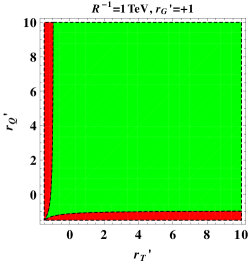
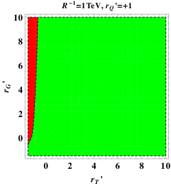
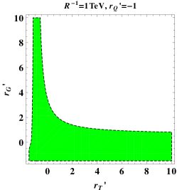
Figure 10: Regions in the $r_{T}^{\prime}-r_{Q}^{\prime}$ (for fixed $r_{G}^{\prime}$; the left-most plot) and $r_{T}^{\prime}-r_{G}^{\prime}$ (for fixed $r_{Q}^{\prime}$; the middle and the right-most plot) planes for $R{{}^{-1}}=1$ TeV that are allowed (in green) by FCNC constraints. For the first two figures, thin strip(s) of the disallowed regions (in red) are highlighted for better visibility.

4.3 Precision constraints

It is well known that the Peskin–Takeuchi parameters $S$, $T$ and $U$ that parametrize the so-called oblique corrections to the electroweak gauge boson propagators Peskin:1990zt ; Peskin:1991sw put rather strong constraints on the mUED scenario. These observables are affected by the modification in the Fermi constant $G_{F}$ (determined experimentally by studying muon decay) due to induced effective 4-fermion vertices originating from exchange of electroweak gauge bosons from even KK levels. These were first calculated in refs. Kakuda:2013kba ; Appelquist:2002wb ; Flacke:2005hb ; Gogoladze:2006br ; Baak:2011ze assuming mUED tree-level spectrum while ref. Flacke:2013pla expressed them in terms of the actual (corrected) masses of the KK modes.

As discussed in refs. Rizzo:1999br ; Davoudiasl:1999tf ; Csaki:2002gy ; Carena:2002dz ; Flacke:2011nb , the correction to $G_{F}$ can be incorporated in the electroweak fit via the modifications it induces in the Peskin–Takeuchi parameters and contrasting them with the experimentally determined values of the latter. Note that in the nmUED scenario we consider, level ‘2’ electroweak gauge bosons have tree-level couplings to the SM fermions and these modify the effective 4-fermion couplings. These effects are over and above what mUED induces where such KK number violating couplings appear only at higher orders. It is thus natural to expect that usual oblique corrections to $S$, $T$ and $U$ induced at one-loop level would be sub-dominant when compared to the above nmUED tree-level contributions. Thus, in our present analysis, we neglect the one-loop contributions but otherwise follow the approach originally adopted in ref. Flacke:2011nb and which was later used in ref. Flacke:2013pla . The nmUED effects are thus parametrized as:

$$S_{\text{nmUED}}=0,\qquad\quad T_{\text{nmUED}}=-\frac{1}{\alpha}\frac{\delta G_{F}}{G_{F}},\qquad\quad U_{\text{nmUED}}=\frac{4\sin^{2}{\theta_{W}}}{\alpha}\frac{\delta G_{F}}{G_{F}}$$ (40)

where $\alpha$ is the electromagnetic coupling strength, $\theta_{W}$ is the $\overline{MS}$ Weinberg angle, both given at the scale $M_{Z}$ and $G_{F}$ is given by

$$G_{F}=G_{F}^{0}+\delta G_{F}$$ (41)

with $G_{F}^{0}$ ($\delta G_{F}$) originating from the $s$-channel SM (even KK) $W^{\pm}$ boson exchange. The concrete forms of these effects are calculated in our model following ref. Flacke:2011nb . Using our notations, these are given by:

$$G_{F}^{0} =\frac{g_{2}^{2}}{4\sqrt{2}}\frac{1}{M_{W}^{2}},\quad\delta G_{F}=\sum_{n\geq 2:\text{even}}\frac{g_{2}^{2}}{4\sqrt{2}}\frac{1}{m_{W_{(n)}}^{2}}\left(g_{{}_{L_{(0)}W_{(n)}L_{(0)}}}\right)^{2},$$ (42)

$$\left.g_{{}_{L_{(0)}W_{(n)}L_{(0)}}}\right|_{n\text{:even}} \equiv\frac{1}{f_{W^{(0)}}}\int_{-L}^{L}dy\left(1+r_{\text{EW}}\left[\delta(y-L)+\delta(y+L)\right]\right)f_{L_{(0)}}f_{W_{(n)}}f_{L_{(0)}}$$

$$=\frac{2\sqrt{4r_{\text{EW}}+2\pi R}\left(M_{W_{(n)}}r_{L}+\tan\left(\frac{M_{W_{(n)}}\pi R}{2}\right)\right)}{M_{W_{(n)}}\left(2r_{L}+\pi R\right)\sqrt{4r_{\text{EW}}+\pi R\sec^{2}\left(\frac{M_{W_{(n)}}\pi R}{2}\right)}+2\tan\left(\frac{M_{W_{(n)}}\pi R}{2}\right)/M_{W_{(n)}}}$$ (43)

where $M_{W_{(n)}}$ is determined by equation 12. Even though the KK leptons do not appear in the process, the BLKT parameter $r_{L}$ in the lepton sector (to be precise, the one for the 5D muon doublet) inevitably influences the coupling-strength given in equation 43. We, however, assume a flavor-universal BLKT parameter $r_{L}$ (just like what we do in the quark sector when we take $r_{Q}=r_{T}$) which help trivially circumvent tree-level contributions to lepton-flavor-violating processes.

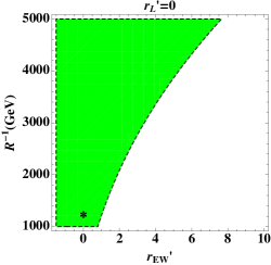
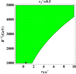
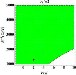
Figure 11: Regions (in green) in the $r_{\text{EW}}^{\prime}-R{{}^{-1}}$ plane allowed by electroweak precision data at $95\%$ C.L. The black asterisks represent the global minimum in each one of them: $\chi^{2}_{\text{min}}=8.8\times 10^{-9}$ at $(r_{\text{EW}}^{\prime},R^{-1})$ = $(6.11\times 10^{-3},1229\,\text{GeV})$ when $r_{L}^{\prime}=0$, $\chi^{2}_{\text{min}}=3.9\times 10^{-9}$ at $(r_{\text{EW}}^{\prime},R^{-1})$ = $(0.505,1029\,\text{GeV})$ when $r_{L}^{\prime}=0.5$, $\chi^{2}_{\text{min}}=1.5\times 10^{-8}$ at $(r_{\text{EW}}^{\prime},R^{-1})$ = $(2.02,1306\,\text{GeV})$ when $r_{L}^{\prime}=2$.

We perform a $\chi^{2}$ fit of the parameters $S_{\text{nmUED}}$, $T_{\text{nmUED}}$ and $U_{\text{nmUED}}$ (with $\delta G_{F}$ evaluated for $n=2$ only) for three fixed values of $r_{L}^{\prime}$ ($r_{L}^{\prime}=r_{L}R{{}^{-1}}=0$, $0.5$ and $2$) to the experimentally fitted values of the allowed new physics (NP) components in these respective observables as reported by the GFitter group Baak:2012kk which are given by

$$S_{\text{NP}}=0.03\pm 0.10, T_{\text{NP}}=0.05\pm 0.12, U_{\text{NP}}=0.03\pm 0.10,$$

the correlation coefficients being

$$\rho_{ST}=+0.89, \rho_{SU}=-0.54, \rho_{TU}=-0.83,$$

and the reference input masses of the SM top quark and the Higgs boson being $m_{t}=173$ GeV and $m_{H}=126$ GeV, respectively.

In figure 11 we show the $95\%$ C.L. allowed region in the $r_{\text{EW}}^{\prime}-R{{}^{-1}}$ plane as a result of the fit performed. As can be expected, the bound refers to $r_{\text{EW}}^{\prime}$ as the only brane-local parameter which, unlike in ref. Flacke:2013pla , can be different from the corresponding parameters governing other sectors of the theory. Such a constraint is going to restrict the mass-spectrum and the couplings in the electroweak sector which is relevant for our present study. It is not unexpected that for larger values of $r_{\text{EW}}$ which result in decreasing masses for the electroweak gauge bosons, only larger values of $R{{}^{-1}}$ (which compensates for the former effect) remain allowed thus rendering these excitations (appearing in the propagators) massive enough to evade the precision bounds. Interestingly, it is possible to relax the bounds by introducing a positive $r_{L}^{\prime}$ as shown in figure 11, a feature that can be taken advantage of as we explore the nmUED parameter space further. This is since the coupling involved $g_{{}_{L_{(0)}W_{(n)}L_{(0)}}}$ gets reduced in the process (see the left plot in figure 5).

4.4 Benchmark scenarios

For our present analysis, we now choose some benchmark scenarios which satisfy the constraints discussed in the previous subsection. The parameter space of these scenarios mainly spans over $r_{T}^{\prime},\,r_{Y}^{\prime},\,R{{}^{-1}}$ and, as a minimal choice, $r_{\text{EW}}^{\prime}=r_{H}^{\prime}$. We also include $r_{G}^{\prime}$, $r_{Q}^{\prime}$ and $r_{L}^{\prime}$ which are the BLKT parameters for the KK gluon, the KK quark and the KK lepton sectors, respectively. $r_{G}^{\prime}$ has some non-trivial implications for the couplings of the KK top quarks to the gluonic excitations as discussed in section 3.4. The parameter $r_{Q}^{\prime}$, though enters our discussion primarily through FCNC considerations (see section 4.2 and appendix B), governs the couplings $V^{(2)}$-$q^{(0)}$-$q^{(0)}$ (as shown in figure 5) that control KK top quark production processes. Both $r_{G}^{\prime}$ and $r_{Q}^{\prime}$ serve as key handles on the masses of the KK gluon and the KK quarks from the first two generations, respectively. Similar is the status of $r_{L}^{\prime}$ which enters through the oblique parameters and controls the masses and couplings in the lepton sector.

In search for suitable benchmark scenarios, we require the following conditions to be satisfied. We require the approximate lower bound on $R{{}^{-1}}$ to hover around 1 TeV which is obtained by recasting the LHC bounds on squarks (from the first two generations) and the gluino in terms of level ‘1’ KK quarks and KK gluons in the nmUED scenario Datta:2012tv . Further, the lighter of the level ‘1’ KK top quark ($t^{(1)}_{l}$) is required to be at least about 500 GeV. This safely evades current LHC-bounds on similar excitations while lower values may still be allowed given that these bounds result from model-dependent assumptions.

The above requirements together calls for a non-minimal sector for the electroweak gauge bosons ($r_{\text{EW}}^{\prime}\neq 0$) such that the lightest KK gauge boson, the KK photon ($\gamma^{(1)}$) is the lightest KK particle (LKP, a possible dark matter candidate). Incorporation of a non-minimal gauge sector affects the couplings of the gauge bosons which, as we will see, could be phenomenologically non-trivial. The choice $r_{\text{EW}}^{\prime}=r_{H}^{\prime}$ renders the KK excitations of the gauge and the Higgs boson very close in mass thus allowing them to take part in the phenomenology of the KK top quarks. In the present scenario, other BLT parameters in the Higgs sector, $\mu_{b}$ and $\lambda_{b}$, are constrained by equations 3 and 11 in addition to the measured Higgs mass as an input. Therefore, these are not independent degrees of freedom.

In table 2 we present the spectra for three such benchmark scenarios: two of them with $R{{}^{-1}}=1$ TeV and the other with $R{{}^{-1}}=1.5$ TeV. The BLKT parameters $r_{G}^{\prime}$ and $r_{Q}^{\prime}$ are so chosen such that the masses of the level ‘1’ KK gluon are in the range 1.6-1.7 TeV (i.e., somewhat above the current LHC lower bounds on similar (SUSY) excitations) while the KK quarks from the first two generations are heavier. Note that in both cases we are having negative $r_{G}^{\prime}$ and $r_{Q}^{\prime}$. In the top quark sector, the BLKT parameter $r_{T}^{\prime}$ are fixed at values for which both light and heavy level ‘1’ KK top quarks have sub-TeV masses and hence expected to be within the LHC reach. Also, $r_{Y}^{\prime}$, the BLT parameter for the Yukawa sector, has been tuned in the process to end up with such spectra. Note that the choices of values for $r_{T}^{\prime}$ and $r_{Y}^{\prime}$ are consistent with the constraints from the physical top quark mass as discussed in section 4.1 and the flavor constraints discussed in section 4.2. Larger values of $R{{}^{-1}}$ would tend to make the level ‘2’ KK top quark a little too heavy (${\lesssim}\,1.5$ TeV) to be explored at the LHC while if one requires the lighter level ‘1’ KK top quark not too light ($\lesssim 300$ GeV) which can be quickly ruled out by the LHC experiments even in an nmUED scenario which we consider. Nonetheless, the lighter of the level ‘2’ top quark may anyway be heavy and only the level ‘1’ top quarks remain to be relevant at the LHC. In that case, larger values of $R{{}^{-1}}$ also remain relevant. Values of $r_{\text{EW}}^{\prime}$ are so chosen as to have $\gamma^{(1)}$ as the LKP with masses around half a TeV. This renders the level ‘2’ electroweak gauge bosons to have masses around 1.5 TeV thus making them possibly sensitive to searches for gauge boson resonances at the LHC Flacke:2012ke ; Chatrchyan:2012su .

In table 2 we also indicate the masses of the level ‘2’ KK excitations. It is to be noted that the lighter of the level ‘2’ KK top quark may not be that heavy ($\lesssim 1.5$ TeV). Level ‘2’ gluon, for our choices of parameters, is pushed to around 3 TeV and hence, unless their couplings to quarks (SM ones or from level ‘1’) are enhanced, LHC may be barely sensitive to their presence. This is a rather involved issue which again warrants dedicated studies and is beyond the scope of the present work.

For the first benchmark point (BM1) with $R{{}^{-1}}=1$ TeV, the mass-splitting between the two level ‘1’ top quark states is much smaller ($\sim 100$ GeV) with a somewhat heavier $t^{(1)}_{l}$ when compared to the second case (BM2) for which $R{{}^{-1}}=1.5$ TeV. We will see in section 5 that such mass-splittings and the absolute masses themselves for the KK top quarks have interesting bearing on their phenomenology at the LHC. Further, the relevant couplings do change (see figures 5, 6 and 7) in going from one point to the other. The third benchmark point BM3 is just BM1 but with different $r_{Y}^{\prime}$ and $m_{t}^{\text{in}}$. BM3 demonstrates a situation with enhanced Higgs-sector couplings and its ramifications at the LHC. It is found that for all the three benchmark points, the coupling $V^{(2)}$-$f^{(0)}$-$f^{(0)}$ get enhanced when level ‘2’ $W$ or $Z$ boson is involved.

Note that the KK bottom quark masses are also governed by $r_{T}^{\prime}$ and $r_{Y}^{\prime}$ for a given $R{{}^{-1}}$. However, since the splitting between the two physical states at a given KK level is proportional to the SM bottom quark mass, the KK bottom quarks at each given level are almost degenerate (just as it is for the KK quark flavors from the first two generations) in mass unlike their top quark counterparts. Thus, some of the KK bottom quarks can have masses comparable to those of the corresponding KK top quark states and hence would eventually enter a collider study otherwise dedicated for the latter. A detailed discussion on the involved issues are out of the scope of the present work.

BM1	$R{{}^{-1}}=1$ TeV, $r_{G}^{\prime}=-1$, $r_{Q}^{\prime}=-1.2$, $r_{T}^{\prime}=1$, $r_{Y}^{\prime}=0.5$, $r_{\text{EW}}^{\prime}=1.5$, $r_{L}^{\prime}=0.4$, $m_{t}^{\text{in}}=173$ GeV
Gauge	$m_{\gamma^{(1)}}=556.9$, $m_{Z^{(1)}}={m_{A^{(1)^{0}}}}=564.4$, $m_{W^{(1)^{\pm}}}={m_{H^{(1)^{\pm}}}}=562.7$, $m_{g^{(1)}}=1653.8$
bosons	$m_{\gamma^{(2)}}=1301.4$, $m_{Z^{(2)}}={m_{A^{(2)^{0}}}}=1304.6$, $m_{W^{(2)^{\pm}}}={m_{H^{(2)^{\pm}}}}=1303.9$, $m_{g^{(2)}}=2780.2$
& Higgs	$m_{H^{(1)^{0}}}=570.8,m_{H^{(2)^{0}}}=1307.4$
	$m_{q^{(1)}}=1711.5$, $m_{q^{(2)}}=2816.9$
Quarks	$m_{t}^{\text{phys}}=172.6$, $m_{t^{(1)}_{l}}=620.4$, $m_{t^{(1)}_{h}}=714.5$
&	$m_{t^{(2)}_{l}}=1359.6$, $m_{t^{(2)}_{h}}=1471.7$
Leptons	$m_{b^{(1)}}=638.3$, $m_{b^{(2)}}=1395.8$
	$m_{l^{(1)}}=802.3$, $m_{l^{(2)}}=1631.8$
BM2	$R{{}^{-1}}=1.5$ TeV, $r_{G}^{\prime}=-0.1$, $r_{Q}^{\prime}=-1.1$, $r_{T}^{\prime}=4$, $r_{Y}^{\prime}=8$, $r_{\text{EW}}^{\prime}=5.5$, $r_{L}^{\prime}=2$, $m_{t}^{\text{in}}=173$ GeV
Gauge	$m_{\gamma^{(1)}}=487.3$, $m_{Z^{(1)}}={m_{A^{(1)^{0}}}}=495.7$, $m_{W^{(1)^{\pm}}}={m_{H^{(1)^{\pm}}}}=493.9$, $m_{g^{(1)}}=1601.6$
bosons	$m_{\gamma^{(2)}}=1655.9$, $m_{Z^{(2)}}={m_{A^{(2)^{0}}}}=1658.4$, $m_{W^{(2)^{\pm}}}={m_{H^{(2)^{\pm}}}}=1657.8$, $m_{g^{(2)}}=3200.8$
& Higgs	$m_{H^{(1)^{0}}}=503.0,m_{H^{(2)^{0}}}=1660.6$
	$m_{q^{(1)}}=2527.5$, $m_{q^{(2)}}=4200.2$
Quarks	$m_{t}^{\text{phys}}=172.4$, $m_{t^{(1)}_{l}}=504.2$, $m_{t^{(1)}_{h}}=813.3$
&	$m_{t^{(2)}_{l}}=1366.3$, $m_{t^{(2)}_{h}}=2220.2$
Leptons	$m_{b^{(1)}}=561.9$, $m_{b^{(2)}}=1706.6$
	$m_{l^{(1)}}=750.0$, $m_{l^{(2)}}=1865.1$
BM3	Input values same as in BM1 except for $r_{Y}^{\prime}=5$ and $m_{t}^{\text{in}}=176$ GeV
Gauge
bosons	Masses same as in BM1
& Higgs
Quarks	Masses same as in BM1 except for $m_{t}^{\text{phys}}=173.4$ and
&	$m_{t^{(1)}_{l}}={626.3}$, $m_{t^{(1)}_{h}}={710.5}$
Leptons	$m_{t^{(2)}_{l}}={1350.7}$, $m_{t^{(2)}_{h}}={1488.6}$

Table 2: Masses (in GeV) of different KK excitations in three benchmark scenarios. With $r_{H}^{\prime}=r_{\text{EW}}^{\prime}$, the level ‘1’ Higgs boson masses are very much similar to the masses of the level ‘1’ electroweak gauge bosons. Choices of the input parameters satisfy the experimental bounds discussed earlier.

5 Phenomenology at the LHC

Given the nontrivial structure of the top quark sector of the nmUED it is expected that the same would have a rich phenomenology at the LHC. A good understanding of the same requires a thorough study of the decay patterns of the KK top quarks and their production rates. In this section we discuss these issues at the lowest order in perturbation theory.

Towards this we implement the scenario in MadGraph 5 Alwall:2011uj using Feynrules version 1 Christensen:2008py via its UFO (Univeral Feynrules Output) Degrande:2011ua ; deAquino:2011ub interface. This now contains the KK gluons, quarks (including the top and the bottom quarks), leptons and the electroweak gauge bosons up to KK level ‘2’. Level ‘1’ and level ‘2’ KK Higgs bosons are also incorporated. The mixings in the quark sector, including ‘level-mixing’ between KK level ‘2’ and level ‘0’, have now been incorporated in a generic way. In this section we discuss these with the help of the benchmark scenarios discussed in section 4.4. We then consolidate the information to summarize the important issues in the search for such excitations at the LHC.

5.1 Decays of the KK top quarks

BM1	$t^{(1)}_{l}\to bW^{(1)^{+}}={0.597}$	$t^{(1)}_{h}\to bW^{(1)^{+}}={0.615}$	$t^{(2)}_{l}\to b^{(1)}_{h}W^{(1)^{+}}={0.351}$
	$bH^{(1)^{+}}={0.403}$	$bH^{(1)^{+}}={0.370}$	$t^{(1)}_{h}A^{(1)^{0}}={0.177}$
		${t^{(1)}_{l}Z=0.016}$	$\boldsymbol{bW^{+}={0.062}}$
			$\boldsymbol{{tH=0.062}}$
			${b^{(1)}_{h}H^{(1)^{+}}=0.057}$
			${b^{(1)}_{l}H^{(1)^{+}}=0.055}$
			$\boldsymbol{{tZ=0.031}}$
BM2	$t^{(1)}_{l}\to bH^{(1)^{+}}={0.842}$	$t^{(1)}_{h}\to b^{(1)}_{h}W^{+}={0.305}$	$t^{(2)}_{l}\to t^{(1)}_{h}A^{(1)^{0}}={0.377}$
	$bW^{(1)^{+}}={0.158}$	$t^{(1)}_{l}Z={0.180}$	$b^{(1)}_{h}H^{(1)^{+}}={0.208}$
		$b^{(1)}_{l}W^{+}={0.141}$	$b^{(1)}_{l}H^{(1)^{+}}={0.200}$
		$tA^{(1)^{0}}={0.130}$	$t^{(1)}_{l}H^{(1)^{0}}={0.109}$
		$t^{(1)}_{l}H={0.126}$	${t^{(1)}_{l}A^{(1)^{0}}=0.055}$
		${bH^{(1)^{+}}=0.069}$	$\boldsymbol{{tH=0.014}}$
		${bW^{(1)^{+}}=0.020}$	$\boldsymbol{{bW^{+}=0.0022}}$
		${tH^{(1)^{0}}=0.015}$	$\boldsymbol{{tZ=0.00058}}$
BM3	$t^{(1)}_{l}\to bH^{(1)^{+}}={0.946}$	$t^{(1)}_{h}\to bH^{(1)^{+}}={0.941}$	$\boldsymbol{t^{(2)}_{l}\to tH={0.448}}$
	$bW^{(1)^{+}}={0.054}$	$bW^{(1)^{+}}={0.060}$	${t^{(1)}_{l}A^{(1)^{0}}=0.102}$
			$t^{(1)}_{h}A^{(1)^{0}}={0.092}$
			${t^{(1)}_{l}H^{(1)^{0}}=0.082}$
			${t^{(1)}_{h}H^{(1)^{0}}=0.063}$
			$\boldsymbol{{bW^{+}=0.046}}$
			$\boldsymbol{{tZ=0.022}}$

Table 3: Decay branching fractions of different KK top quarks for the three benchmark points presented in table 2. Modes having branching fractions less than about a percent are not presented except for the ones with a pair of SM particles in the final state. Tree level decays of $t^{(2)}_{l}$ to SM states are shown in bold in the right-most column.

Decays of the KK top quarks are mainly governed by the two input parameters, $r_{T}^{\prime}$ and $r_{\text{EW}}^{\prime}$, for a given value of $R{{}^{-1}}$. The dependence is rather involved since these two parameters not only determine the spectra of the KK top quarks and the KK electroweak gauge bosons but also the involved couplings. The latter, in turn, are complicated functions of the input parameters as given by equation 39 and as illustrated in figures 5, 6 and 7. In the following, we briefly discuss the possible decay modes of the KK top quarks and the significance of some of them at the LHC. In table 3 we list the branching fractions for the three benchmark points presented earlier in table 2.

For our choices of input parameters, two decay modes are possible for $t^{(1)}_{l}$: $t^{(1)}_{l}\to bW^{(1)^{+}}$ and $t^{(1)}_{l}\to bH^{(1)^{+}}$. Decays to $tZ^{(1)}/t\gamma^{(1)}/tH^{(1)^{0}}/tA^{(1)^{0}}$ are also possible when the mass-splitting between $t^{(1)}_{l}$ and $Z^{(1)}/\gamma^{(1)}/H^{(1)^{0}}/A^{(1)^{0}}$ is larger than the mass of the SM-like top quark. In our scenario, its decays to $b^{(1)}_{l}$ and $b^{(1)}_{h}$ are prohibited on kinematic grounds. Unlike in some competing scenarios (like the MSSM) where channels like, say, $\tilde{t}_{1}\to b\chi^{+}_{1}$ and $\tilde{t}_{1}\to t\chi^{0}_{1}$) could attain a 100% branching fraction, the spectra of the involved KK excitations in our scenario would not allow $t^{(1)}_{l}$ decaying exclusively to either $bW^{(1)^{\pm}}$ or $t\gamma^{(1)}$. The reason behind this is that $W^{(1)^{\pm}}$ and $\gamma^{(1)}$ are rather close in mass and hence if decays to $t\gamma^{(1)}$ is allowed, the same to $bW^{(1)^{+}}$ is also kinematically possible. Further, even the latter mode has to compete with $t^{(1)}_{l}\to bH^{(1)^{+}}$ as $m_{W^{(1)^{\pm}}}\approx m_{H^{(1)^{\pm}}}$. Translating constraints on such KK top quarks from those obtained in the LHC-studies of, say, the top squarks is not at all straight-forward since the latter explicitly assume either $\tilde{t}_{1}\to b\chi^{+}_{1}=100\%$ Aad:2013ija ; Chatrchyan:2013xna or $\tilde{t}_{1}\to t\chi^{0}_{1}=100\%$ Chatrchyan:2013xna . Further, $W^{(1)^{\pm}}$ (and also $Z^{(1)}$), being among the lighter most ones of all the level ‘1’ KK excitations, would only undergo three-body decays to LKP ($\gamma^{(1)}$) accompanied by leptons or jets that would be rather soft because of the near-degeneracy of the masses of the level ‘1’ KK gauge bosons. This would lead to loss of experimental sensitivity for final states with more number of hard leptons and jets Aad:2013ija .

The situation with $t^{(1)}_{h}$ is not qualitatively much different as long as decay modes similar to $t^{(1)}_{l}$ are the dominant ones. This is the case with BM1. Under such circumstances, they could turn out to be reasonable backgrounds to each other (if their production rates are comparable) and dedicated studies would be required to disentangle them. In any case (even in the absence of good discriminators), simultaneous productions of both $t^{(1)}_{l}$ and $t^{(1)}_{h}$ would enhance the new-physics signal. On the other hand, in a situation like BM2, more decay modes may be available to $t^{(1)}_{h}$ although decays to level ‘1’ bottom and top quarks along with SM $W^{\pm}$ and $Z$ are the dominant ones. The ensuing cascades of these states would inevitably make the analysis challenging. However, under favorable circumstances, reconstructions of the $W^{\pm}$ and/or $Z$ bosons along with $b$- and/or top-tagging could help disentangle the signals. Thus, it appears that search for level ‘1’ KK top quarks involves complicated issues (some of which are common to top squark searches in SUSY scenarios) and a multi-channel analysis could turn out to be very effective.

We now turn to the case of level ‘2’ top KK top quarks. The lighter of the two states, $t^{(2)}_{l}$ can have substantial rates at the LHC which is discussed in some detail in section 5.2. This motivates us to study the decay patterns of $t^{(2)}_{l}$. In the last column of table 3 we present the decay branching fractions of $t^{(2)}_{l}$. As can be seen, the decay modes that are usually enhanced involve a pair of level ‘1’ KK excitations which would cascade to the LKP. We, however, strive to understand to what extent $t^{(2)}_{l}$, being an even KK-parity state, could decay directly to a pair of comparatively light (level ‘0’) particles (and hence, boosted) comprising of an SM fermion and an SM gauge/Higgs boson. Thus, in the one hand, these decay products are unlikely to be missed in an experiment while on the other hand, new techniques to reconstruct (like the study of jet substructure Altheimer:2012mn ; Dasgupta:2013ihk etc.) some of them have to be employed.

In scenario BM1, the total decay branching fraction to SM states (shown in bold) is just about 15% while in scenario BM2 such decays are practically absent. Given the large phase space available, such small (or non-existent) decay rates to SM particles can only be justified in terms of rather feeble (effective) couplings among the involved states. The couplings of $t^{(2)}_{l}$ to the SM gauge bosons and an SM fermion would have vanished (due to the orthogonality of the mode functions involved) had $t^{(2)}_{l}$ been a pure level ‘2’ state. The smallness of these couplings thus readily follows from the tiny admixture of the SM top quark in the physical $t^{(2)}_{l}$ state and thus, results in its small branching fractions to SM gauge bosons. The same argument does not hold for the corresponding coupling $t^{(2)}_{l}$-$t$-$H$ that controls the other SM decay mode of $t^{(2)}_{l}$, i.e., $t^{(2)}_{l}\to tH$. However, it is clear from figure 7 that this coupling is going to be small for both the benchmark points BM1 and BM2.

Since direct decays of $t^{(2)}_{l}$ to SM states could provide the ‘smoking guns’ at the LHC in the form of rather boosted objects (top and bottom quarks, $Z$, $W^{\pm}$ and Higgs boson) that could eventually be reconstructed to their parent, this motivates us to study if such decays can ever become appreciable. We find that the coupling $t^{(2)}_{l}$-$t$-$H$ gets significantly enhanced with a slight modification in the parameters of BM1 (called BM3 in table 2) by setting $r_{Y}^{\prime}=5$ (see figure 7) and $m_{t}^{\text{in}}=176$ GeV while keeping other parameters untouched and still satisfying all the experimental constraints that we discussed. As we can see, the branching fraction to $tH$ final state could attain a level of 50% which should be healthy for the purpose. Efficient tagging of boosted top quarks Kaplan:2008ie ; CMS:2009lxa ; Plehn:2011tg ; Schaetzel:2013vka and boosted Higgs bosons Butterworth:2008iy would hold the key in such a situation. Some such techniques have already been proposed in recent literature Berger:2012ec , in particular, in the context of vector-like top quarks or more generally, in the study of ‘top-partners’.

On the other hand, since the $t^{(2)}_{l}$-$t$-$Z$ and $t^{(2)}_{l}$-$b$-$W^{\pm}$ are dynamically constrained, these could only get enhanced if the competing modes (decays to a pair of level ‘1’ KK states) face closure. As the couplings involved in the latter cases are generically of SM strength, these could only be effectively suppressed by having them kinematically forbidden. From figure 12 we find that, by itself, this is not very difficult to achieve (in yellow shade) over the nmUED parameter space. However, rather conspicuously, the simultaneous demands for the KK photon to be the LKP with $m_{\gamma^{(1)}}>400$ GeV (the red-shaded region) and that of $m_{t^{(2)}_{l}}<1.5$ TeV (in blue shade) leave no overlapping region in the nmUED parameter space. It may appear that one simple way to find some overlap is by moving down in $r_{T}^{\prime}$. However, this implies $t^{(2)}_{l}$ becomes more massive thus loosing in its production cross section in the first place. Although the interplay of events that leads to this kind of a situation is not an easy thing to follow, the issue that is broadly conspiring is the similarity in the basic evolution-pattern of the masses of the KK excitations as functions of the BLKT parameters (see figure 2 and ref. Datta:2012tv ).

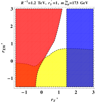
Figure 12: Region in $r_{T}^{\prime}-r_{\text{EW}}^{\prime}$ plane where the decays $t^{(2)}_{l}\to t^{(1)}_{l}\gamma^{(1)},\,t^{(1)}_{l}Z^{(1)},\,b^{(1)}_{l}W^{(1)^{+}}$ are kinematically prohibited (in yellow), $\gamma^{(1)}$ is the LKP with $m_{\gamma^{(1)}}>400$ GeV (in red) and $m_{t^{(2)}_{l}}<1.5$ TeV (in blue). The entire region shown is compatible with the acceptable range of the mass of the top quark and other precision constraints.

5.2 Production processes

In this section we discuss different production modes of the KK top quarks at the 14 TeV (the design energy) LHC with reference to the nmUED parameter space. These are of following four broad types (in line with top squark phenomenology in SUSY scenarios):

• the generic mode with two top quark excitations in the final state that receives contributions from processes involving both strong and electroweak interactions,

• exclusively electroweak processes leading to a single top quark excitation

• the associated production of a pair of KK top quarks and the (SM) Higgs boson and

• production from the cascades of KK gluons and KK quarks.

5.2.1 Final states with a pair of top quark excitations

These are the processes where two similar or different kind of top quark excitations are produced in the final state. The interesting modes in this category are pair-production of $t^{(1)}_{l}$ and $t^{(1)}_{h}$ along with the associated productions of $t^{(1)}_{l}t^{(1)}_{h}$ and $t^{(2)}_{l}t$. The latter two processes are possible in an nmUED scenario and the corresponding Feynman diagrams are presented in figure 13. Note that the requirement of current conservation does not allow the massless SM gauge bosons (gluon and photon) to mediate these processes while the pair-productions receive contributions from all possible mediations. Also, these two associated production modes have no counter-parts in a competing SUSY scenario like the MSSM.

In figure 14 we illustrate the variations of the rates for these processes with $r_{T}^{\prime}$ for $R{{}^{-1}}$=1 TeV (left) and 2 TeV (right). As can be seen, pair production of $t^{(1)}_{l}$, has by far the largest cross section for $r_{T}^{\prime}\gtrsim 3$ reaching up to 10 (1) pb for $R{{}^{-1}}$ = 1.5 (2) TeV. This is not unexpected since $t^{(1)}_{l}$ is the lightest of the KK top quarks. In this regime, the yields for $t^{(1)}_{h}$-pair and $t^{(1)}_{l}t^{(1)}_{h}$ associated productions are very similar touching 1 (0.1) pb for $R{{}^{-1}}$ = 1.5 (2) TeV. The corresponding rates for $t^{(2)}_{l}t$ associated production do not lag much notching 0.5 (0.05) pb, respectively. Further, the $t^{(2)}_{l}$-pair has a trend similar to that of the $t^{(1)}_{l}$-pair in this respect but, rate-wise, falls out of the competition.

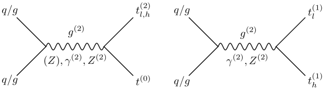
Figure 13: Feynman diagrams for the associated $t^{(2)}_{l}-t^{(0)}$ (left) and $t^{(1)}_{l}-t^{(1)}_{h}$ productions at the LHC. The gluon-initiated processes are only mediated by $g^{(2)}$ while the quark-initiated processes are mediated by both $g^{(2)}$ and other electroweak gauge bosons from level ‘0’ ($Z$) and level ‘2’ ($\gamma^{(2)},\,Z^{(2)}$).

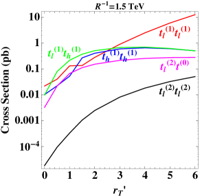
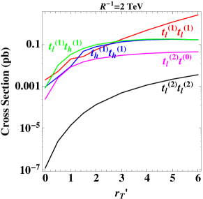
Figure 14: Cross sections (in picobarns, at tree level) for different production processes involving the KK top quarks as functions of $r_{T}^{\prime}$ at the 14 TeV LHC for $R{{}^{-1}}=1.5$ TeV (left) and $R{{}^{-1}}=2$ TeV (right), $r_{Y}^{\prime}=3$, $r_{G}^{\prime}=0.5$ and the other parameters are chosen as in the BM2. CTEQ6L1 parton distributions Nadolsky:2008zw are used and the factorization/renormalization scale is set at the sum of the masses in the final state.

Note that with increasing $r_{T}^{\prime}$ masses of all the KK states decrease. Interestingly enough, this effect is reflected in a straight-forward manner only in the case of $t^{(1)}_{l}$-pair for which the rates increase with growing $r_{T}^{\prime}$. For other competing processes mentioned above, the curves flatten out. This behavior signals non-trivial interplays of the intricate couplings involved. These have much to do with when all these rates become comparable for $r_{T}^{\prime}\lesssim 3$. In the process, the rate for usual $t\bar{t}$ pair production also gets affected to some extent. However, our estimates are all being at the tree level, these do not pose any immediate concern while facing the measured $t\bar{t}$ cross section which is much larger and agrees with its estimation at higher orders in perturbation theory. Also, in table 4 we present the cross sections for the three benchmark points.

The bottom-line is that the production rates of three different KK top quark excitations remain moderately healthy over favorable region of the nmUED parameter space at a future LHC run. With the knowledge of their decay patterns (see table 3) and the associated features discussed in section 5.1 it is required to chalk out a strategy to reach out to these excitations.

Benchmark	$t^{(1)}_{l}\bar{t}^{(1)}_{l}$	$t^{(1)}_{l}\bar{t}^{(1)}_{h}$	$t^{(1)}_{h}\bar{t}^{(1)}_{h}$	$t\bar{t}^{(2)}_{l}$
	(pb)	(pb)	(pb)	(pb)
BM1	0.63	0.10	0.35	0.07
BM2	2.24	0.35	0.76	0.21
BM3	0.76	0.11	0.30	0.07

Table 4: Production cross sections (in picobarns, at tree level) for different pairs of KK top quarks for the benchmark points. Contributions from the Hermitian conjugate processes are taken into account wherever applicable. The choices for the parton distribution and the scheme for determining the factorization/renormalization scale are the same as in figure 14.

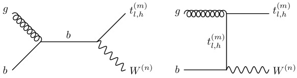
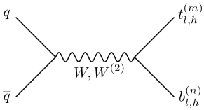
Figure 15: Generic Feynman diagrams for the single production of a KK top quark along with KK excitations of $W^{\pm}$ boson (upper panel) and KK bottom quark (lower panel) at the LHC. Superscripts $m$ and $n$ standing for the KK levels can be different (like ‘0’ and ‘2’) but should ensure KK-parity conservation.

5.2.2 Single production processes

We consider two broad categories of single production of KK top quarks which are closely analogous to single top production in the SM once the issue of KK-parity conservation is taken into account. In the first case, a level ‘1’ KK top quark is produced in association with level $W^{(1)^{\pm}}$ or $b^{(1)}$ quark. The second one involves the lighter of the level ‘2’ KK top quarks along with an SM $W^{\pm}$ boson or an SM bottom quark. The generic, tree-level Feynman diagrams that contribute to the processes are presented in figure 15.

Benchmark	$t^{(1)}_{l}W^{(1)^{-}}$	$t^{(1)}_{l}\bar{b}^{(1)}_{l}$	$t^{(2)}_{l}b$	$t^{(1)}_{l}\bar{t}^{(1)}_{l}H$	$t^{(1)}_{l}\bar{t}^{(1)}_{h}H$	$t^{(1)}_{h}\bar{t}^{(1)}_{h}H$	$t\bar{t}^{(2)}_{l}H$	$t\bar{t}H$
	(pb)	(pb)	(pb)	(pb)	(pb)	(pb)	(pb)	(pb)
BM1	0.01	0.11	0.11	$\sim 10^{-5}$	$\sim 10^{-4}$	$\sim 10^{-3}$	0.03	0.24
BM2	0.04	0.21	0.13	0.73	5.39	0.17	0.11	1.25
BM3	$\sim 10^{-3}$	0.23	0.11	$\sim 10^{-4}$	$\sim 10^{-3}$	0.01	0.04	2.21

Table 5: Cross sections (in picobarns, at tree level) for single and (SM) Higgs-associated KK top quark productions for the benchmark points. The mass of the SM Higgs boson is taken to be 125 GeV. Contributions from the Hermitian conjugate processes are taken into account wherever applicable. The choices for the parton distribution and the scheme for determining the factorization/renormalization scale are the same as in figure 14.

Single production of level ‘1’ top quarks:

Single production of level ‘1’ top quarks along with a level ‘1’ $W^{\pm}$ boson proceeds via $gb$ fusion in $s$-channel and $gb$ scattering in $t$-channel. The rates are at best a few tens of femtobarns as can be seen from table 5. On the other hand, the mode in which a level ‘1’ bottom quark is produced in association proceeds through $s$-channel fusion of light quarks and propagated by $W^{\pm}$ and $W^{(2)^{\pm}}$ bosons. The cross sections are found to be rather healthy ranging from 110 fb to 230 fb. The observed rates for $t^{(1)}_{l}W^{(1)^{\pm}}$ production appear to be consistently lower than that for $t^{(1)}_{l}b^{(1)}_{l}$ production. This can be traced back to the presence of enhanced $q$-$q^{\prime}$-$W^{(2)^{\pm}}$ coupling. Moreover, cross sections for other combinations involving heavier states of $t^{(1)}$ and $b^{(1)}$ in the final state could have comparable strengths because of such enhanced couplings.

Single production of level ‘2’ top quark:

The associated $t^{(2)}_{l}W^{-}$ production involves the vertex $t^{(2)}_{l}$-$W^{\pm}$-$b$ which, as we discussed earlier (see sections 3.4.1 and 5.1), vanishes but for a small admixture of level ‘0’ top in the physical state $t^{(2)}$. Hence, the rates in this mode turn out to be insignificant. Further, the $W^{\pm}$-mediated diagram in the associated $t^{(2)}_{l}b$ production also has the same vertex and thus contributes negligibly. The only contribution here comes from the diagram mediated by $W^{(2)^{\pm}}$ which is somewhat massive. Thus, the prospect of having healthy rates for the single production of $t^{(2)}$ depends entirely on the coupling strength $t^{(2)}_{l}$-$W^{(2)^{\pm}}$-$b$ and $W^{(2)^{\pm}}$-$q$-$q$ (see figure 5). Fortunately, this is the case here and the cross sections for all three benchmark points, as can be seen from table 5, are above and around 100 fb.

We also looked into the production of $t^{(2)}_{l}$ along with light quark jets which is analogous to, by far the most dominant, ‘$t$-channel’ single top production process (the so-called $W$-gluon fusion process) in the SM. However, in our scenario, such a process with somewhat heavy $t^{(2)}_{l}$ yields a few tens of a femtobarn for all the three benchmark points.

For both the categories mentioned above, the new-physics contributions to the corresponding SM processes are systematically small. This is since these contain the couplings that involve level-mixing effect in the top-quark sector which is not large.

5.2.3 Associated production of KK top quarks with the SM Higgs boson

The associated Higgs production processes we consider involve both light and heavy level ‘1’ top quarks in pairs and the level ‘2’ lighter top quark along with the SM top quark. The generic tree level Feynman diagrams are presented in figure 16. Given that the study of the SM $t\bar{t}H$ production is by itself complicated enough, it is only natural to expect that the same with its KK counterparts would not be any simpler.

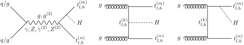
Figure 16: Generic Feynman diagrams for the associated (SM) Higgs production along with a pair of KK excitations of the top quark. Superscripts $k$, $m$ and $n$ can be different (like ‘0’ and ‘2’) but should ensure KK-parity conservation.

Cross sections for such processes are listed in table 5 for the benchmark points we consider. To have a feel about the their phenomenological prospects, these can be compared with similar processes in the SM and a SUSY scenario like the MSSM. In the MSSM, the lowest order cross section is around a few tens of a fb for the process $\tilde{t}_{1}\tilde{t}^{*}_{1}H$ with $m_{\tilde{t}_{1}}\approx 300$ GeV and for the most favorable values of the involved couplings Djouadi:1997xx ; Djouadi:2005gj while for the SM the corresponding rate is about 430 fb Beenakker:2001rj ; Djouadi:2005gi . It is encouraging to find that the yield for $tt^{(2)}_{l}H$ is either comparable (for BM1 and BM3) or larger (BM2) than what can at best be expected in MSSM. Note that the level ‘1’ lighter KK top quark is somewhat heavier (with mass around or above 500 GeV) for our benchmark points when compared to the mass of the top squark as indicated above. For other processes, BM2 consistently leads to larger cross sections. The interplay of different Feynman diagrams (see figure 16) along with the modified strengths of the participating gauge and Yukawa interactions play roles in some such enhancements.

In the last column of table 5 we indicate the lowest order cross sections for the SM process $t\bar{t}H$ which now gets affected in an nmUED scenario. Note that for BM1 the cross section is smaller than the SM value of $\approx 430$ fb while for BM2 and BM3 the same is about 3 and 5 times as large, respectively. Such deviations can be expected if we refer back to the left panel of figure 7 that illustrates how the $t$-$\bar{t}$-$H$ coupling gets modified over the nmUED parameter space. Note that, non-observation of such a process at the LHC, till recently, could only restrict the rate up to around five times the SM rate Chatrchyan:2013yea ; cms-tth-gamma ; atlas-tth-gamma . Thus, benchmark point BM3, as such, can be considered as a borderline case. But given that $t\bar{t}H$ cross section depends on other nmUED parameters like $r_{G}^{\prime}$, $r_{Q}^{\prime}$ etc., one could easily circumvent this restriction without requiring a compromise with the parameters like $r_{T}^{\prime}$ and $r_{Y}^{\prime}$ that define the essential feature of BM3, i.e., the enhanced couplings among the top quark excitations and the SM Higgs boson. It is interesting to find that in favorable regions of parameter space, the cross section for Higgs production in association with a pair of rather heavy KK top quarks could compare with or even exceed the $t\bar{t}H$ cross section. Note that in the MSSM, such enhancement only happens for large mixing in the stop sector and when $m_{\tilde{t}_{1}}<m_{t}$ Djouadi:2005gj .

Further, once the level ‘1’ KK Higgs bosons are taken up for studies, the associated production of a charged KK Higgs boson (from level ‘1’) in the final state $bt^{(1)}_{l}H^{{(1)}^{\pm}}$ would become rather relevant and may turn out to be interesting as the total mass involved in this final state can be comparatively much lower. The prospect there depends crucially on the strength of the involved 3-point vertex though.

5.2.4 Production of KK top quarks under cascades

KK gluon(s) and quarks, once produced, can cascade to KK top quarks. This would result in multiple top quarks (upto four of them) in the final state at the LHC. In our benchmark scenarios where $m_{g^{(1)}}<m_{q^{(1)}}$, KK gluons would directly decay to KK top quarks while KK quarks from the first two generations would undergo a two-step decay via KK gluon to yield a KK top quark. The latter one has thus suppressed contribution. We find that the branching fraction for $g^{(1)}\to t^{(1)}t$ is around 50% for all three benchmark points (the rest 50% is to level ‘1’ bottom quark states). With strong production rates for the $g^{(1)}$-pair, $g^{(1)}q^{(1)}$ and $q^{(1)}$-pair ranging between 0.01 pb to 2.6 pb (in increasing order), the yield of a single level ‘1’ KK top final state could be anywhere between 10 fb to a few pb. These seem quite healthy. However, one has to cope with backgrounds which now have enhanced level of jet activity.

6 Conclusions and outlook

We discuss the structure and the phenomenology of the top quark sector in a scenario with one flat extra spatial dimension orbifolded on $S^{1}/Z_{2}$ and containing non-vanishing BLTs. The discussion inevitably draws reference to the gauge and the Higgs sectors. The scenario, by construct, preserves KK-parity.

The main purpose of the present work is to organize and work out (following ref. Flacke:2008ne ) the necessary details in the involved sectors and explore the salient features with their broad phenomenological implications in terms of a few benchmark scenarios. This lay down the basis for future, detailed studies of such a top quark sector at the LHC.

The masses and the couplings of the Kaluza-Klein excitations are estimated at the lowest order in perturbation theory as functions of $R{{}^{-1}}$ and the BLT parameters. For the KK top quarks, the extended mixing scheme (originating in the Yukawa sector) is thoroughly worked out by incorporating level-mixing among the level ‘0’ and the level ‘2’ KK top quark states, a phenomenon that is not present in the popular mUED scenario. In addition, unlike in the mUED, tree-level couplings that violate KK-number (but conserve KK-parity) are possible. We demonstrate how all these new effects, together, attract constraints from different precision experiments and shape the phenomenology of such a scenario.

The nmUED scenario we consider has eight free parameters: $R{{}^{-1}}$ and the scaled (by $R{{}^{-1}}$) BLT coefficients $r_{Q}^{\prime}$, $r_{L}^{\prime}$, $r_{T}^{\prime}$, $r_{Y}^{\prime}$, $r_{G}^{\prime}$, $r_{\text{EW}}^{\prime}\,(=r_{W}^{\prime}=r_{B}^{\prime}=r_{H}^{\prime})$ and $m_{t}^{\text{in}}$. However, in the present study, the most direct roles are played by $r_{T}^{\prime}$, $r_{Y}^{\prime}$ and $r_{\text{EW}}^{\prime}$ (=$r_{H}^{\prime}$) in conjunction with $R{{}^{-1}}$. $r_{Q}^{\prime}$ and $r_{G}^{\prime}$ play roles in the production processes by determining some relevant gauge-fermion couplings beside controlling the KK quark and gluon masses, respectively. On the other hand, $r_{L}^{\prime}$ and $m_{t}^{\text{in}}$ only play some indirect roles through their influence on the experimentally measured effects that determine the allowed region of the parameter space.

The scenario has been thoroughly implemented in MadGraph 5. Three benchmark scenarios that satisfy all the relevant experimental constraints are chosen for our study. These give conservatively light KK spectra with sub-TeV masses for both level ‘1’ electroweak KK gauge bosons (with $\gamma^{(1)}$ as the LKP) and the KK top quarks while having the lighter level ‘2’ top quark below 1.5 TeV thus making them all relevant at the LHC. Level ‘1’ KK quarks from the first two generations and the KK gluon are taken to be heavier than 1.6 TeV.

Near mass-degeneracy of the electroweak KK gauge bosons and the KK Higgs bosons (at a given KK level) is a feature. This influences the decays of the KK top quarks. The lighter of the level ‘1’ KK top quark can never decay 100% of the time to a top quark and the LKP photon. This is in sharp contrast to a similar possibility in a SUSY scenario like the MSSM when a top squark can decay 100% of the time to a top quark and the LSP neutralino, an assumption that is frequently made by the LHC collaborations. Instead, such a KK top quark has significant branching fractions to both charged KK Higgs boson and to KK $W$ bosons at the same time. Further, split between the KK top quark and the KK electroweak gauge bosons that is attainable in the nmUED scenario would generically lead to hard primary jets in the decays of the former. This is again in clear contrast to the mUED scenario. However, near mass-degeneracy prevailing in the gauge and the Higgs sector would still result in rather soft leptons/secondary jets. Limited mass-splitting among the KK gauge and Higgs bosons is a possibility that has non-trivial ramifications and hence needs closer scrutiny.

The level ‘2’ KK top quark we consider can decay directly to much lighter SM particles like the $W$, the $Z$, the Higgs boson and the top quark. These would then be boosted and hence may serve as ‘smoking guns’. Recent studies of the vector-like top partners CMS:2012ab ; ATLAS:2012qe ; atlas:heavytop are in context. However, these studies mainly bank on their pair-production and decays that comprise only of pairs of SM particles like $bW^{\pm}$ and/or $tZ$ and/or $tH$. In the nmUED model that we consider, these are always accompanied by other modes that may be dominant as well. The level ‘2’ top quark decaying to a pair of level ‘1’ KK states is one such example.

Thus, phenomenology of the KK top quarks could turn out to be rather rich (and complex) at the LHC. Clearly, strategies tailor-made for searches of similar excitations under different scenarios could at best be of very limited use. Even recasting the analyses for some of them to the nmUED scenario is not at all straight-forward. This calls for a dedicated strategy that incorporates optimal triggers and employs advanced techniques like analysis of jet-substructures etc. to tag the boosted objects in the final states.

In any case, viability of a dedicated hunt depends crucially on optimal production rates. We study these for the 14 TeV run of the LHC. For all the possible modes in which KK top quarks can be produced (like the pair-production, the single production and the associated production with the SM Higgs boson), the rates are found to be rather encouraging and may even exceed the corresponding MSSM processes, a yard-stick that can perhaps be used safely (with a broad brush, though) for the purpose.

The LHC experiments are either already sensitive or will be achieving the same soon in the next run for all the generic processes discussed in this work. Given that the nmUED provides several top quark KK excitations with different characteristic decays and production rates, the sensitivity to them can only be increased if multi-channel searches are carried out. It is thus possible that the LHC, running at its design energy of 14 TeV (or even a little less), finds some of these states. However, concrete studies with rigorous detector-level simulations are prerequisites to chalking out a robust strategy.

Last but not the least, the intimate connection between the top quark and the Higgs sectors raises genuine curiosity in the phenomenology for the KK Higgs bosons as well. The nmUED Higgs sector holds good promise for a rather rich phenomenology at the LHC which has become further relevant after the discovery of the ‘SM-like’ Higgs boson and hence can turn out to be a fertile area to embark upon.

Acknowledgments KN and SN are partially supported by funding available from the Department of Atomic Energy, Government of India for the Regional Centre for Accelerator-based Particle Physics (RECAPP), Harish-Chandra Research Institute. The authors like to thank Benjamin Fuks for very helpful discussions on issues with FeynRules and SN thanks Ujjal Kumar Dey for many helpful discussions. The authors acknowledge the use of computational facility available at RECAPP and thank Joyanto Mitra for technical help.

Appendix A Gauge and the Higgs sector of the nmUED: some relevant details

In this appendix we briefly supplement our discussion in section 2.1 with some necessary details pertaining to the gauge fixing conditions, the inputs that go into the mass-determining conditions.

A.1 Gauge fixing conditions

We introduce the gauge-fixing terms in the bulk and at the boundaries in the following way to obtain the physical states:

$$S_{\text{gf}} =\int d^{4}x\int_{-L}^{L}dy\Bigg{\{}-\frac{1}{2\xi_{A}}\left[\partial_{\mu}A^{\mu}-\xi_{A}\partial_{y}A_{y}\right]^{2}-\frac{1}{\xi_{W}}\left|\partial_{\mu}W^{+\mu}-\xi_{W}\left(\partial_{y}W_{y}^{+}+iM_{W}\phi^{+}\right)\right|^{2}$$

$$\phantom{=\int d^{4}x\int_{-L}^{L}dy\Bigg{\{}\,\,}-\frac{1}{2\xi_{Z}}\left[\partial_{\mu}Z^{\mu}-\xi_{Z}\left(\partial_{y}Z_{y}+M_{Z}\chi\right)\right]^{2}-\frac{1}{2\xi_{G}}\left[\partial_{\mu}G^{a\mu}-\xi_{G}\partial_{y}G_{y}^{a}\right]^{2}$$

$$-\frac{1}{2\xi_{A,b}}\Big{\{}\left[\partial_{\mu}A^{\mu}+\xi_{A,b}A_{y}\right]^{2}\delta(y-L)+\left[\partial_{\mu}A^{\mu}-\xi_{A,b}A_{y}\right]^{2}\delta(y+L)\Big{\}}$$

$$-\frac{1}{\xi_{W,b}}\Big{\{}\left|\partial_{\mu}W^{+\mu}+\xi_{W,b}\left(W_{y}^{+}-ir_{H}M_{W}\phi^{+}\right)\right|^{2}\delta(y-L)+\left|\partial_{\mu}W^{+\mu}-\xi_{W,b}\left(W_{y}^{+}+ir_{H}M_{W}\phi^{+}\right)\right|^{2}\delta(y+L)\Big{\}}$$

$$-\frac{1}{2\xi_{Z,b}}\Big{\{}\left[\partial_{\mu}Z^{\mu}+\xi_{Z,b}\left(Z_{y}-r_{H}M_{Z}\chi\right)\right]^{2}\delta(y-L)+\left[\partial_{\mu}Z^{\mu}-\xi_{Z,b}\left(Z_{y}+r_{H}M_{Z}\chi\right)\right]^{2}\delta(y+L)\Big{\}}$$

$$-\frac{1}{2\xi_{G,b}}\Big{\{}\left[\partial_{\mu}G^{a\mu}+\xi_{G,b}G_{y}^{a}\right]^{2}\delta(y-L)+\left[\partial_{\mu}G^{a\mu}-\xi_{G,b}G_{y}^{a}\right]^{2}\delta(y+L)\Big{\}}\Bigg{\}}$$ (44)

where the eight gauge-fixing parameters are $\xi_{A},\,\xi_{W},\,\xi_{Z},\,\xi_{G}$ (in the bulk), $\xi_{A,b},\,\xi_{W,b},\,\xi_{Z,b},\,\xi_{G,b}$ (at the boundary) and $M_{W},\,M_{Z}$ are the masses of the $W$ and $Z$ bosons.

Imposing the unitary gauge in both the bulk and at the boundaries by setting

$$\xi_{A},\,\xi_{W},\,\xi_{Z},\,\xi_{G},\,\xi_{A,b},\,\xi_{W,b},\,\xi_{Z,b},\,\xi_{G,b}\to\infty$$ (45)

we obtain the following relations:

$$A_{y} =0, Z_{y}\mp r_{H}M_{Z}\chi =0,$$

$$W_{y}^{+}\mp ir_{H}M_{W}\phi^{+} =0, G_{y}^{a} =0,\qquad\text{at }y=\pm L,$$ (46)

$$\partial_{y}A_{y} =0, \partial_{y}W_{y}^{+}+iM_{W}\phi^{+} =0,$$

$$\partial_{y}Z_{y}+M_{Z}\chi =0, \partial_{y}G_{y}^{a} =0,\qquad\text{in the bulk}.$$ (47)

As we see, $A_{y}$ and $G_{y}^{a}$ are totally gauged away from the theory as would-be Nambu-Goldstone bosons. The two mixed boundary conditions in equation 46 can be cast into a set containing the individual fields with the help of equation 47 as

$$\chi\pm r_{H}\partial_{y}\chi =0, \phi^{+}\pm r_{H}\partial_{y}\phi^{+} =0,$$

$$Z_{y}\pm r_{H}\partial_{y}Z_{y} =0, W_{y}^{+}\pm r_{H}\partial_{y}W_{y}^{+} =0,\qquad\text{at }y=\pm L.$$ (48)

A.2 Input parameters for masses of the the KK gauge and Higgs bosons

Input parameters that determine the masses of the KK gauge and the Higgs bosons of the nmUED Flacke:2008ne (as solutions for the conditions given in equation (8)) are presented in table 6.

Type	$m_{F}^{2}$	$m_{F,b}^{2}$	$r_{F}$
$W_{\mu}^{+}$	$M_{W}^{2}$	$r_{H}M_{W}^{2}$	$r_{\text{EW}}$
$Z_{\mu}$	$M_{Z}^{2}$	$r_{H}M_{Z}^{2}$	$r_{\text{EW}}$
$H$	$(\sqrt{2}\hat{\mu})^{2}$	$(\sqrt{2}\mu_{b})^{2}$	$r_{H}$
$\phi^{+},\,\partial_{y}W_{y}^{+}$	$M_{W}^{2}$	$r_{H}M_{W}^{2}$	$r_{H}$
$\chi,\,\partial_{y}Z_{y}$	$M_{Z}^{2}$	$r_{H}M_{Z}^{2}$	$r_{H}$

Table 6: Input parameters that determine the masses of the KK gauge and Higgs bosons. See section 2.1 for notations and conventions.

Appendix B Tree-level FCNCs, the “aligned” scenario and constraints from $D^{0}-\overline{D^{0}}$ mixing

It has been demonstrated in ref. gerstenlauer that an appropriate short-distance description for a $\Delta F$=2 FCNC process like $D^{0}-\overline{D^{0}}$ can be found in processes involving only the even KK modes (starting at level ‘2’) of the gauge bosons and the ‘0’ mode fermions. In an effective Hamiltonian approach, such a process would reduce to a four-Fermi interaction whose strength is suppressed by the mass of the exchanged KK gauge boson. The effective FCNC Hamiltonian can be expressed in terms of suitable fermionic operators and their associated Wilson coefficients. The latter involve the overlap matrices in the gauge kinetic terms (by now, suitably rotated to the basis where the quark mass matrix is diagonal) which are functions of the BLKT parameter, $r_{Q}^{\prime}$ and $r_{T}^{\prime}$. Thus, any constraint on the Wilson coefficients can be translated into constraints in the $r_{Q}^{\prime}$-$r_{T}^{\prime}$ plane.

The gauge interactions in the diagonalized basis involving the level ‘0’ quarks and the KK gluons $g^{(k)}$, with the KK index $k$ being even and $k\geq 2$, are given by:

$$g_{s}\sum_{i,j,l=1}^{3}\bigg{(}\overline{q^{(0)}_{iL}}\gamma^{\mu}T^{a}\Big{[}(U_{qL}^{\dagger})_{il}F^{Q,[k]}_{g,ll}(U_{qL})_{lj}\Big{]}q^{(0)}_{jL}+\overline{q^{(0)}_{iR}}\gamma^{\mu}T^{a}\Big{[}(U_{qR}^{\dagger})_{il}F^{q,[k]}_{g,ll}(U_{qR})_{lj}\Big{]}q^{(0)}_{jR}\bigg{)}g_{\mu}^{(k)},$$ (49)

where the 4D and the 5D (the ‘hatted’ one) gauge couplings are related by $g_{s}\,\equiv\,\hat{g}_{s}/\sqrt{2r_{G}+\pi R}$. $T^{a}$ represents the $SU(3)$ generators, $a$ being the color index. $U_{q(L,R)}$ are the matrices that diagonalize the $q_{L,R}$ fields in the Yukawa sector. $F^{Q,[k]}_{g,ll}$ and $F^{q,[k]}_{g,ll}$ are the diagonal overlap matrices (in the original bases)

$$F^{Q,[k]}_{g,ll} =\frac{1}{f_{g^{(0)}}}\int_{-L}^{L}dy\left(1+r_{Q_{l}}\left[\delta(y-L)+\delta(y+L)\right]\right)f_{Q^{(0)}_{l}}f_{g^{(k)}}f_{Q^{(0)}_{l}},$$ (50)

$$F^{q,[k]}_{g,ll} =\frac{1}{f_{g^{(0)}}}\int_{-L}^{L}dy\left(1+r_{q_{l}}\left[\delta(y-L)+\delta(y+L)\right]\right)f_{q^{(0)}_{l}}f_{g^{(k)}}f_{q^{(0)}_{l}}$$ (51)

while the explicit form is shown in equation 43. Similar FCNC processes are also induced by the KK photons and the KK $Z$ bosons. However, because of weaker couplings their contributions are only sub-leading and henceforth neglected in the present work.

The so-called “aligned” scenario in which the rotation matrices for the left- and the right-handed quark fields are tuned to avoid as many flavor constraints as possible can be summarized as

$$U_{uR} =U_{dR}=U_{dL}={\bf 1}_{3}, U_{uL} =V_{\text{CKM}}^{\dagger}$$ (52)

along with universal BLKT parameters $r_{Q}^{\prime}$ and $r_{T}^{\prime}$, for the first two and the third quark generations respectively, irrespective of their chiralities. In such a scenario, by construct, dominant tree-level FCNC is induced via KK gluon exchange and only through the doublet up-quark sector. Note that no FCNC appears at the up-quark singlet part and the down-quark sector. The latter helps evade severe bounds from the $K$ and $B$ meson sectors. The forms of the 4D Yukawa couplings, before diagonalization, are determined simultaneously as:

$$Y^{u}_{ij}=\sum_{l=1}^{3}\frac{\left(V_{\text{CKM}}^{\dagger}\right)_{il}\mathcal{Y}^{u}_{lj}}{F^{d,(0,0)}_{ij}},\qquad Y^{d}_{ij}=\begin{cases}\displaystyle\frac{\mathcal{Y}^{d}_{ii}}{F^{d,(0,0)}_{ii}}&\text{for}\ i=j,\\ \displaystyle 0&\text{for}\ i\not=j.\end{cases}$$ (53)

In this configuration, the structure of the vertex $\overline{u^{(0)}_{iL}}-d^{(0)}_{jL}-W^{+(0)}_{\mu}$ is reduced to that of the SM. The overlap matrices in the gauge kinetic sector receive bi-unitary transformations when these terms are rotated to a basis where the quark mass matrices in the Yukawa sector are diagonal. These rotated overlap matrices are given by

$$\sum_{l=1}^{3}(U_{uL}^{\dagger})_{il}F^{U,[k]}_{g,ll}(U_{uL})_{lj} =\left\{F^{U,[k]}_{g,11}{\bf 1}_{3}+V_{\text{CKM}}\begin{pmatrix}0&&\\ &0&\\ &&\underbrace{F^{U,[k]}_{g,33}-F^{U,[k]}_{g,11}}_{=:\Delta F^{U,[k]}_{g}}\end{pmatrix}V_{\text{CKM}}^{\dagger}\right\}_{ij}$$

$$\simeq\left\{F^{U,[k]}_{g,11}{\bf 1}_{3}+\Delta F^{U,[k]}_{g}\begin{pmatrix}A^{2}\lambda^{6}&-A^{2}\lambda^{5}&A\lambda^{3}\\ -A^{2}\lambda^{5}&A^{2}\lambda^{4}&-A\lambda^{2}\\ A\lambda^{3}&-A\lambda^{2}&1\end{pmatrix}\right\}_{ij}$$ (54)

where $A(=0.814)$ and $\lambda(=0.23)$ are the usual Wolfenstein parameters and we use the relation $F^{U,[k]}_{g,11}=F^{U,[k]}_{g,22}$. Clearly, the difference of the two overlap matrices in that diagonal term governs the FCNC contribution and thus, in turn, relative values of the corresponding BLKT parameters, $r_{Q}^{\prime}$ and $r_{T}^{\prime}$ that shape the overlap matrices, get constrained.

To exploit the model independent constraints provided by the UTfit collaboration Bona:2007vi , the effective Hamiltonian for the $t$-channel KK gluon exchange process (that describes the $D^{0}-\overline{D^{0}}$ mixing effect) needs to be written down in terms of the following quark operators and the associated Wilson coefficient:

$$\Delta\mathcal{H}_{\text{eff}}^{\Delta C=2}=C_{D}^{1}(\overline{u}^{a}_{L}\gamma_{\mu}c^{a}_{L})(\overline{u}^{b}_{L}\gamma^{\mu}c^{b}_{L})$$ (55)

where $a$ and $b$ are the color indices and we use $SU(3)$ algebra and appropriate Fierz transformation to obtain

$$C_{D}^{1}=\sum_{k\geq 2:\text{even}}\frac{g_{s}^{2}(\mu_{D})}{6}\frac{1}{m_{g^{(2)}}^{2}}(-A^{2}\lambda^{5}\Delta F^{U,[k]}_{g})^{2}\simeq\frac{2\pi\alpha_{s}(\mu_{D})}{3m_{g^{(2)}}^{2}}A^{4}\lambda^{10}(\Delta F^{U,[k]}_{g})^{2}.$$ (56)

As it appears, the value of $C_{D}^{1}$ is highly Cabibbo-suppressed. Heavier KK gluons (except the one from level ‘2’) effectively decouples. The QCD coupling at the $D^{0}$-meson scale $(\mu_{D}\simeq 2.8\,\text{GeV})$ is estimated by the relation,

$$\alpha^{-1}_{s}(\mu_{D})=\alpha^{-1}_{s}(M_{Z})-\frac{1}{6\pi}\left(23\ln{\frac{M_{Z}}{m_{b}}}+25\ln{\frac{m_{b}}{\mu_{D}}}\right)\simeq 1/0.240$$ (57)

with $\alpha_{s}(M_{Z})=0.1184$ Adachi:2011tn . One would now be able to put bounds on the parameter space by use of the result by the UTfit collaboration Bona:2007vi ,

$$|C^{1}_{D}|<7.2\times 10^{-7}\,\text{TeV}^{-2}$$ (58)

which, for a given set of values for $R{{}^{-1}}$ and $r_{G}^{\prime}$, actually exploits the dependence of $\Delta F^{U,[k]}_{g}$ (appearing in equation (B.6)) on the BLKT parameters $r_{Q}^{\prime}$ and $r_{T}^{\prime}$.

References

- (1) F. Del Aguila and J. Santiago, “Signals from extra dimensions decoupled from the compactification scale,” JHEP 0203 (2002) 010 [hep-ph/0111047].
- (2) H. -C. Cheng, K. T. Matchev and M. Schmaltz, “Bosonic supersymmetry? Getting fooled at the CERN LHC,” Phys. Rev. D 66 (2002) 056006 [hep-ph/0205314].
- (3) F. J. Petriello, “Kaluza-Klein effects on Higgs physics in universal extra dimensions,” JHEP 0205 (2002) 003 [hep-ph/0204067].
- (4) S. K. Rai, “UED effects on Higgs signals at LHC,” Int. J. Mod. Phys. A 23 (2008) 823 [hep-ph/0510339].
- (5) N. Maru, T. Nomura, J. Sato and M. Yamanaka, “Higgs Production via Gluon Fusion in a Six Dimensional Universal Extra Dimension Model on ,” Eur. Phys. J. C 66 (2010) 283 [arXiv:0905.4554 [hep-ph]].
- (6) K. Nishiwaki, “Higgs production and decay processes via loop diagrams in various 6D Universal Extra Dimension Models at LHC,” JHEP 1205 (2012) 111 [arXiv:1101.0649 [hep-ph]].
- (7) K. Nishiwaki, K. -y. Oda, N. Okuda and R. Watanabe, “A Bound on Universal Extra Dimension Models from up to 2fb-1 of LHC Data at 7 TeV,” Phys. Lett. B 707 (2012) 506 [arXiv:1108.1764 [hep-ph]].
- (8) K. Nishiwaki, K. -y. Oda, N. Okuda and R. Watanabe, “Heavy Higgs at Tevatron and LHC in Universal Extra Dimension Models,” Phys. Rev. D 85 (2012) 035026 [arXiv:1108.1765 [hep-ph]].
- (9) G. Belanger, A. Belyaev, M. Brown, M. Kakizaki and A. Pukhov, “Testing Minimal Universal Extra Dimensions Using Higgs Boson Searches at the LHC,” Phys. Rev. D 87 (2013) 016008 [arXiv:1207.0798 [hep-ph]].
- (10) U. K. Dey and T. S. Ray, “Constraining minimal and non-minimal UED models with Higgs couplings,” Phys. Rev. D 88 (2013) 056016 [arXiv:1305.1016 [hep-ph]].
- (11) T. Kakuda, K. Nishiwaki, K. -y. Oda and R. Watanabe, “Universal extra dimensions after Higgs discovery,” Phys. Rev. D 88 (2013) 035007 [arXiv:1305.1686 [hep-ph]].
- (12) T. Flacke, K. Kong and S. C. Park, “126 GeV Higgs in Next-to-Minimal Universal Extra Dimensions,” arXiv:1309.7077 [hep-ph].
- (13) T. Appelquist, H. -C. Cheng and B. A. Dobrescu, “Bounds on universal extra dimensions,” Phys. Rev. D 64 (2001) 035002 [hep-ph/0012100].
- (14) H. C. Cheng, K. T. Matchev and M. Schmaltz, “Radiative corrections to Kaluza-Klein masses,” Phys. Rev. D 66 (2002) 036005 [hep-ph/0204342].
- (15) I. Antoniadis, “A Possible new dimension at a few TeV,” Phys. Lett. B 246 (1990) 377.
- (16) F. del Aguila, M. Perez-Victoria and J. Santiago, “Bulk fields with general brane kinetic terms,” JHEP 0302 (2003) 051 [hep-th/0302023].
- (17) F. del Aguila, M. Perez-Victoria and J. Santiago, “Bulk fields with brane terms,” Eur. Phys. J. C 33 (2004) S773 [hep-ph/0310352].
- (18) F. del Aguila, M. Perez-Victoria and J. Santiago, “Effective description of brane terms in extra dimensions,” JHEP 0610 (2006) 056 [hep-ph/0601222].
- (19) Y. Fujimoto, T. Nagasawa, K. Nishiwaki and M. Sakamoto, “Quark mass hierarchy and mixing via geometry of extra dimension with point interactions,” PTEP 2013 (2013) 023B07 [arXiv:1209.5150 [hep-ph]].
- (20) Y. Fujimoto, K. Nishiwaki and M. Sakamoto, “CP phase from twisted Higgs VEV in extra dimension,” arXiv:1301.7253 [hep-ph].
- (21) A. Datta, K. Nishiwaki and S. Niyogi, “Non-minimal Universal Extra Dimensions: The Strongly Interacting Sector at the Large Hadron Collider,” JHEP 1211 (2012) 154 [arXiv:1206.3987 [hep-ph]].
- (22) A. Datta, U. K. Dey, A. Shaw and A. Raychaudhuri, “Universal Extra-Dimensional Models with Boundary Localized Kinetic Terms: Probing at the LHC,” Phys. Rev. D 87 (2013) 076002 [arXiv:1205.4334 [hep-ph]].
- (23) A. Datta, A. Raychaudhuri and A. Shaw, “LHC limits on KK-parity non-conservation in the strong sector of universal extra-dimension models,” arXiv:1310.2021 [hep-ph].
- (24) D. Choudhury, A. Datta and K. Ghosh, “Deciphering Universal Extra Dimension from the top quark signals at the CERN LHC,” JHEP 1008 (2010) 051 [arXiv:0911.4064 [hep-ph]].
- (25) J. A. Aguilar-Saavedra, “Identifying top partners at LHC,” JHEP 0911, 030 (2009) [arXiv:0907.3155 [hep-ph]].
- (26) G. Cacciapaglia, A. Deandrea, D. Harada and Y. Okada, “Bounds and Decays of New Heavy Vector-like Top Partners,” JHEP 1011, 159 (2010) [arXiv:1007.2933 [hep-ph]].
- (27) G. Cacciapaglia, A. Deandrea, L. Panizzi, N. Gaur, D. Harada and Y. Okada, “Heavy Vector-like Top Partners at the LHC and flavour constraints,” JHEP 1203, 070 (2012) [arXiv:1108.6329 [hep-ph]].
- (28) J. Berger, J. Hubisz and M. Perelstein, “A Fermionic Top Partner: Naturalness and the LHC,” JHEP 1207 (2012) 016 [arXiv:1205.0013 [hep-ph]].
- (29) A. De Simone, O. Matsedonskyi, R. Rattazzi and A. Wulzer, “A First Top Partner Hunter’s Guide,” JHEP 1304 (2013) 004 [arXiv:1211.5663 [hep-ph]].
- (30) J. Kearney, A. Pierce and J. Thaler, “Top Partner Probes of Extended Higgs Sectors,” JHEP 1308 (2013) 130 [arXiv:1304.4233 [hep-ph]].
- (31) M. Buchkremer, G. Cacciapaglia, A. Deandrea and L. Panizzi, “Model Independent Framework for Searches of Top Partners,” Nucl. Phys. B 876 (2013) 376 [arXiv:1305.4172 [hep-ph]].
- (32) J. A. Aguilar-Saavedra, R. Benbrik, S. Heinemeyer and M. Perez-Victoria, “A handbook of vector-like quarks: mixing and single production,” Phys. Rev. D 88, 094010 (2013) [arXiv:1306.0572 [hep-ph]].
- (33) F. del Aguila, M. Perez-Victoria and J. Santiago, “Some consequences of brane kinetic terms for bulk fermions,” hep-ph/0305119.
- (34) F. del Aguila, M. Perez-Victoria and J. Santiago, “Physics of brane kinetic terms,” Acta Phys. Polon. B 34 (2003) 5511 [hep-ph/0310353].
- (35) T. Flacke, A. Menon and D. J. Phalen, “Non-minimal universal extra dimensions,” Phys. Rev. D 79 (2009) 056009 [arXiv:0811.1598 [hep-ph]].
- (36) P. Bandyopadhyay, B. Bhattacherjee and A. Datta, “Search for Higgs bosons of the Universal Extra Dimensions at the Large Hadron Collider,” JHEP 1003 (2010) 048 [arXiv:0909.3108 [hep-ph]].
- (37) S. Chatrchyan et al. [CMS Collaboration], “Search for the standard model Higgs boson produced in association with a top-quark pair in collisions at the LHC,” JHEP 1305 (2013) 145 [arXiv:1303.0763 [hep-ex]].
- (38) CMS Collaboration, “Search for ttH production in events where decays to photons at 8 TeV collisions”, CMS-PAS-HIG-13-015.
- (39) ATLAS collaboration, “Search for production in the channel at TeV with the ATLAS detector”, ATLAS-CONF-2013-080.
- (40) K. Nishiwaki, S. Niyogi and A. Shivaji, “ Anomalous Coupling in Double Higgs Production,” arXiv:1309.6907 [hep-ph].
- (41) S. Alekhin, A. Djouadi and S. Moch, “The top quark and Higgs boson masses and the stability of the electroweak vacuum,” Phys. Lett. B 716 (2012) 214 [arXiv:1207.0980 [hep-ph]].
- (42) CDF [Tevatron Electroweak Working Group and D0 Collaborations], “Combination of CDF and DO results on the mass of the top quark using up to 8.7 fb-1 at the Tevatron,” arXiv:1305.3929 [hep-ex].
- (43) Diploma thesis by D. Gerstenlauer, “Flavor Physics in Universal Extra Dimension Models with Brane Kinetic Localized Terms,” Universität Würzburg, May 2011.
- (44) R Aaij et al. [LHCb Collaboration], “Observation of oscillations,” Phys. Rev. Lett. 110 (2013) 101802 [arXiv:1211.1230 [hep-ex]].
- (45) M. Bona et al. [UTfit Collaboration], “Model-independent constraints on F=2 operators and the scale of new physics,” JHEP 0803, 049 (2008) [arXiv:0707.0636 [hep-ph]].
- (46) M. E. Peskin and T. Takeuchi, “A New constraint on a strongly interacting Higgs sector,” Phys. Rev. Lett. 65 (1990) 964.
- (47) M. E. Peskin and T. Takeuchi, “Estimation of oblique electroweak corrections,” Phys. Rev. D 46 (1992) 381.
- (48) T. Appelquist and H. -U. Yee, “Universal extra dimensions and the Higgs boson mass,” Phys. Rev. D 67 (2003) 055002 [hep-ph/0211023].
- (49) T. Flacke, D. Hooper and J. March-Russell, “Improved bounds on universal extra dimensions and consequences for LKP dark matter,” Phys. Rev. D 73 (2006) 095002 [Erratum-ibid. D 74 (2006) 019902] [hep-ph/0509352].
- (50) I. Gogoladze and C. Macesanu, “Precision electroweak constraints on Universal Extra Dimensions revisited,” Phys. Rev. D 74 (2006) 093012 [hep-ph/0605207].
- (51) M. Baak, M. Goebel, J. Haller, A. Hoecker, D. Ludwig, K. Moenig, M. Schott and J. Stelzer, “Updated Status of the Global Electroweak Fit and Constraints on New Physics,” Eur. Phys. J. C 72 (2012) 2003 [arXiv:1107.0975 [hep-ph]].
- (52) T. Flacke, K. Kong and S. C. Park, “Phenomenology of Universal Extra Dimensions with Bulk-Masses and Brane-Localized Terms,” JHEP 1305 (2013) 111 [arXiv:1303.0872 [hep-ph]].
- (53) T. G. Rizzo and J. D. Wells, “Electroweak precision measurements and collider probes of the standard model with large extra dimensions,” Phys. Rev. D 61 (2000) 016007 [hep-ph/9906234].
- (54) H. Davoudiasl, J. L. Hewett and T. G. Rizzo, “Bulk gauge fields in the Randall-Sundrum model,” Phys. Lett. B 473 (2000) 43 [hep-ph/9911262].
- (55) C. Csaki, J. Erlich and J. Terning, “The Effective Lagrangian in the Randall-Sundrum model and electroweak physics,” Phys. Rev. D 66 (2002) 064021 [hep-ph/0203034].
- (56) M. S. Carena, E. Ponton, T. M. P. Tait and C. E. M Wagner, “Opaque branes in warped backgrounds,” Phys. Rev. D 67 (2003) 096006 [hep-ph/0212307].
- (57) T. Flacke and C. Pasold, “Constraints on split-UED from Electroweak Precision Tests,” Phys. Rev. D 85, 126007 (2012) [arXiv:1111.7250 [hep-ph]].
- (58) M. Baak, M. Goebel, J. Haller, A. Hoecker, D. Kennedy, R. Kogler, K. Moenig and M. Schott et al., “The Electroweak Fit of the Standard Model after the Discovery of a New Boson at the LHC,” Eur. Phys. J. C 72, 2205 (2012) [arXiv:1209.2716 [hep-ph]].
- (59) T. Flacke, A. Menon and Z. Sullivan, “Constraints on UED from searches,” Phys. Rev. D 86 (2012) 093006 [arXiv:1207.4472 [hep-ph]].
- (60) S. Chatrchyan et al. [CMS Collaboration], “Search for charge-asymmetric production of ’ bosons in top pair + jet events from collisions at TeV,” Phys. Lett. B 717 (2012) 351 [arXiv:1206.3921 [hep-ex]].
- (61) R. Kelley, L. Randall and B. Shuve, “Early (and Later) LHC Search Strategies for Broad Dimuon Resonances,” JHEP 1102 (2011) 014 [arXiv:1011.0728 [hep-ph]].
- (62) J. Alwall, M. Herquet, F. Maltoni, O. Mattelaer and T. Stelzer, “MadGraph 5 : Going Beyond,” JHEP 1106 (2011) 128 [arXiv:1106.0522 [hep-ph]].
- (63) N. D. Christensen and C. Duhr, “FeynRules - Feynman rules made easy,” Comput. Phys. Commun. 180 (2009) 1614 [arXiv:0806.4194 [hep-ph]].
- (64) C. Degrande, C. Duhr, B. Fuks, D. Grellscheid, O. Mattelaer and T. Reiter, “UFO - The Universal FeynRules Output,” Comput. Phys. Commun. 183 (2012) 1201 [arXiv:1108.2040 [hep-ph]].
- (65) P. de Aquino, W. Link, F. Maltoni, O. Mattelaer and T. Stelzer, “ALOHA: Automatic Libraries Of Helicity Amplitudes for Feynman Diagram Computations,” Comput. Phys. Commun. 183 (2012) 2254 [arXiv:1108.2041 [hep-ph]].
- (66) G. Aad et al. [ATLAS Collaboration], “Search for direct third-generation squark pair production in final states with missing transverse momentum and two b-jets in =8 TeV collisions with the ATLAS detector,” arXiv:1308.2631 [hep-ex].
- (67) S. Chatrchyan et al. [CMS Collaboration], “Search for top-squark pair production in the single-lepton final state in collisions at TeV,” arXiv:1308.1586 [hep-ex].
- (68) A. Altheimer, S. Arora, L. Asquith, G. Brooijmans, J. Butterworth, M. Campanelli, B. Chapleau and A. E. Cholakian et al., “Jet Substructure at the Tevatron and LHC: New results, new tools, new benchmarks,” J. Phys. G 39 (2012) 063001 [arXiv:1201.0008 [hep-ph]].
- (69) M. Dasgupta, A. Fregoso, S. Marzani and G. P. Salam, “Towards an understanding of jet substructure,” JHEP 1309 (2013) 029 [arXiv:1307.0007 [hep-ph]].
- (70) D. E. Kaplan, K. Rehermann, M. D. Schwartz and B. Tweedie, “Top Tagging: A Method for Identifying Boosted Hadronically Decaying Top Quarks,” Phys. Rev. Lett. 101 (2008) 142001 [arXiv:0806.0848 [hep-ph]].
- (71) [CMS Collaboration], “A Cambridge-Aachen (C-A) based Jet Algorithm for boosted top-jet tagging,” CMS-PAS-JME-09-001.
- (72) T. Plehn and M. Spannowsky, “Top Tagging,” J. Phys. G 39 (2012) 083001 [arXiv:1112.4441 [hep-ph]].
- (73) S. Schaetzel and M. Spannowsky, “Tagging highly boosted top quarks,” arXiv:1308.0540 [hep-ph].
- (74) J. M. Butterworth, A. R. Davison, M. Rubin and G. P. Salam, “Jet substructure as a new Higgs search channel at the LHC,” Phys. Rev. Lett. 100 (2008) 242001 [arXiv:0802.2470 [hep-ph]].
- (75) D. Binosi and L. Theussl, “JaxoDraw: A Graphical user interface for drawing Feynman diagrams,” Comput. Phys. Commun. 161 (2004) 76 [hep-ph/0309015].
- (76) J. A. M. Vermaseren, “Axodraw,” Comput. Phys. Commun. 83 (1994) 45.
- (77) P. M. Nadolsky, H. -L. Lai, Q. -H. Cao, J. Huston, J. Pumplin, D. Stump, W. -K. Tung and C. -P. Yuan, “Implications of CTEQ global analysis for collider observables,” Phys. Rev. D 78 (2008) 013004 [arXiv:0802.0007 [hep-ph]].
- (78) A. Djouadi, J. L. Kneur and G. Moultaka, “Higgs boson production in association with scalar top quarks at proton colliders,” Phys. Rev. Lett. 80 (1998) 1830 [hep-ph/9711244].
- (79) A. Djouadi, “The Anatomy of electro-weak symmetry breaking. II. The Higgs bosons in the minimal supersymmetric model,” Phys. Rept. 459 (2008) 1 [hep-ph/0503173] and references therein.
- (80) W. Beenakker, S. Dittmaier, M. Kramer, B. Plumper, M. Spira and P. M. Zerwas, “Higgs radiation off top quarks at the Tevatron and the LHC,” Phys. Rev. Lett. 87 (2001) 201805 [hep-ph/0107081].
- (81) A. Djouadi, “The Anatomy of electro-weak symmetry breaking. I: The Higgs boson in the standard model,” Phys. Rept. 457 (2008) 1 [hep-ph/0503172] and references therein.
- (82) S. Chatrchyan et al. [CMS Collaboration], “Search for heavy, top-like quark pair production in the dilepton final state in collisions at TeV,” Phys. Lett. B 716 (2012) 103 [arXiv:1203.5410 [hep-ex]].
- (83) G. Aad et al. [ATLAS Collaboration], “Search for pair production of heavy top-like quarks decaying to a high-pT boson and a quark in the lepton plus jets final state at =7 TeV with the ATLAS detector,” Phys. Lett. B 718 (2013) 1284 [arXiv:1210.5468 [hep-ex]].
- (84) [ATLAS Collaboration], “Search for pair production of heavy top-like quarks decaying to a high- boson and a quark in the lepton plus jets final state in collisions at TeV with the ATLAS detector”, ATLAS-CONF-2013-060.
- (85) Y. Adachi, N. Kurahashi, C. S. Lim and N. Maru, “ Mixing in Gauge-Higgs Unification,” JHEP 1201, 047 (2012) [arXiv:1103.5980 [hep-ph]].