Conformal invariance of the 3D self-avoiding walk

Abstract

We show that if the three dimensional self-avoiding walk (SAW) is conformally invariant, then one can compute the hitting densities for the SAW in a half space and in a sphere. We test these predictions by Monte Carlo simulations and find excellent agreement, thus providing evidence that the SAW is conformally invariant in three dimensions.

In two dimensions the self-avoiding walk (SAW) is believed to be conformally invariant, and this leads to a rich set of predictions. In particular the scaling limit of the SAW in a simply connected domain between two fixed points is predicted to be the Schramm-Lowener evolution with $\kappa=8/3$ lsw_saw . For SAW’s in a domain which start at a fixed point but are allowed to end anywhere on the boundary, there are predictions for the distribution of the terminal point lsw_saw . Simulations of the SAW have found excellent agreement with these predictions Kennedya ; Kennedyb ; kennedy_lawler .

In two dimensions the extensive predictions for the SAW can be seen as a consequence of the large group of conformal transformations. In three and higher dimensions this group is rather modest; it is generated by Euclidean symmetries and inversions in spheres. Nonetheless it is still nontrivial, and the use of conformal invariance to study critical systems in more than two dimensions has a long history. In particular, conformal invariance was used to study the SAW in cardy1984conformal ; cardyredner . So it is natural to ask if the scaling limit of the SAW is conformally invariant in three and more dimensions, and if such invariance would yield any information about the SAW. Since this scaling limit has been proved to be Brownian motion in more than four dimensions hara_slade_a ; hara_slade_b and substantial progress toward proving this for four dimensions has been made bs , this question is most interesting in three dimensions. In this paper we show that despite the rather limited set of conformal transformations in three dimensions, conformal invariance allows one to make some nontrivial predictions. We test these predictions by simulations of the SAW and find excellent agreement.

The probability of a SAW $\omega$ is taken to be proportional to $\mu^{-N}$ where $N$ is the number of steps and $\mu$ is the lattice connectivity constant for the SAW, i.e., the reciprocal of the critical fugacity. $N$ is not constrained, and there are a variety of grand canonical ensembles that we will use. We can consider all SAW’s in the full space that go between two fixed points. We can consider all SAW’s in a domain $D$ with a variety of possible constraints on the endpoints. In the chordal ensemble the two endpoints are fixed points on the boundary of $D$. In the radial ensemble one endpoint is a fixed point on the boundary and the other is a fixed point in the interior. Finally, we can consider an ensemble in which one endpoint is a fixed point in the interior but the other endpoint can be anywhere on the boundary of the domain. In this ensemble the location of the endpoint on the boundary is random, and we refer to its density as the hitting density. In all these ensembles the SAW is initially defined on a lattice with spacing $\delta$, and we let $\delta\rightarrow 0$ to obtain the scaling limit. For background on the SAW we refer the reader to des1990polymers , and for the SAW near a surface to eisenriegler1993polymers .

We will use several critical exponents for the SAW. Let $N$ denote the number of steps in the SAW $\omega$, so $\omega(N)$ is the endpoint of the SAW. The exponent $\nu$ characterizes the growth of the SAW with the number of steps. Letting $<\quad>$ denote expectation with respect to the uniform probability measure on SAW’s with $N$ steps starting at the origin, $<||\omega(N)||^{2}>\sim N^{2\nu}$. The number of SAW’s with $N$ steps starting at the origin grows as $\mu^{N}N^{\gamma-1}$ where $\mu$ depends on the lattice but the exponent $\gamma$ does not. If we only allow SAW’s that stay in a half-plane ($d=2$) or a half-space ($d=3$), then it grows like $\mu^{N}N^{\gamma-1-\rho}$. ($\gamma-\rho$ is often denoted by $\gamma_{1}$.) So the probability that a SAW with N steps in the full space lies in the half space goes like $N^{-\rho}$. The final exponent we will need is the boundary scaling exponent $b$. In the chordal ensemble of SAW’s between two fixed points on the boundary, the partition function will go to zero like $\delta^{2b}$ as the lattice spacing $\delta\rightarrow 0$. The exponent $b$ is related to the field theory exponent $\eta_{\parallel}$ that describes the decay of spin-spin correlation along the boundary by $\eta_{\parallel}=2b$. Another characterization of $b$ in two dimensions is that the probability the SAW will pass through a slit of width $\epsilon$ in a curve will go as $\epsilon^{2b}$ as the width goes to zero. In three dimensions the probability the SAW will pass through a small hole in a surface will go as $l^{2b}$ where $l$ is the linear size of the hole. So it will go as $\epsilon^{b}$ if $\epsilon$ is the area. A well known scaling relation between these four exponents in $d$ dimensions is $2b\nu=2\rho-\gamma+d\nu$. A non-rigorous derivation for the SAW may be found in lsw_saw .

In two dimensions there are exact, but unproven, predictions for these exponents: $\nu=3/4$ flory , $\gamma=43/32$ nienhuis , $\rho=25/64$ cardy1984conformal and $b=\eta_{\parallel}/2=5/8$ cardy1984conformal . In three dimensions there are numerical estimates but no exact predictions: $\nu=0.587597(7)$ clisby_nu , $\gamma=1.15698(34)$ gamma_schram , $\gamma_{1}=0.679\pm 0.002$ where $\gamma_{1}=\gamma-\rho$ hegger_grassberger .

The chordal and radial ensembles of the SAW are believed to be conformally invariant. The ensemble in which the SAW starts at a point in the interior and ends anywhere on the boundary is not. The hitting density for this ensemble is conformally covariant. Since this density is uniform when the SAW starts at the center of a disc, this conformal covariance completely determines the hitting density for simply connected two dimensional domains. We give a derivation of the Lawler, Schramm, Werner formula lsw_saw for the conformal covariance of the hitting density in two dimensions since our results in three dimensions will follow the same argument.

Let $D$ be a simply connected domain. Let $C$ be a simple curve between two boundary points. It divides $D$ into two subdomains which we call $A$ and $B$. Let $a$ be a boundary point of the subdomain $A$ which is not on $C$, and $b$ a boundary point of the subdomain $B$, not on $C$. See fig. 1. We consider the SAW in $D$ from $a$ to $b$ and condition on the event that it crosses $C$ only once. This is conditioning on an event with probability zero, so we must do it by a limiting process. We look at the event that there is a segment of width $\epsilon$ in $C$ such that the curve hits $C$ only in this segment. Then we let $\epsilon\rightarrow 0$. The probability of passing through a slit of width $\epsilon$ should go to zero like $\epsilon^{2b}$. The prefactor will depend on where we are along the curve and it is this prefactor that we interpret as the unnormalized probability that the SAW crosses $C$ at that point given that it crosses $C$ only once. We denote it by

$$\pi_{D,C,a,b}(z)=\lim_{\epsilon\rightarrow 0}\epsilon^{-2b}\,P(\epsilon\,slit\,at\,z)$$

where $\epsilon\,slit\,at\,z$ stands for the event that the SAW passes through a slit of width $\epsilon$ centered at a point $z\in C$.

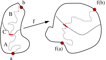
Figure 1:

Now let ${f}(z)$ be a conformal map on $D$. By conformal invariance, the probability the SAW in $D$ goes through the slit in $C$ at $z$ is the same as the probability that the SAW in ${f}(D)$ from ${f}(a)$ to ${f}(b)$ goes through a slit in ${f}(C)$ at ${f}(z)$ of width $|{f}^{\prime}(z)|\epsilon$. This change of the width of the slit is crucial. Equating the two probabilities and canceling the common factor of $\epsilon^{2b}$, we have

$$\pi_{D,C,a,b}(z)=\pi_{{f}(D),{f}(C),{f}(a),{f}(b)}({f}(z))\,|{f}^{\prime}(z)|^{2b}$$ (1)

Summing over all SAW’s in $D$ that go through a slit should be the same as the product of the sum over all SAW’s in $A$ from $a$ to the slit times the sum over all SAW’s in $B$ from $b$ to the slit. Let $\sigma_{A,C,a}(z)$ denote the hitting density for a SAW in $A$ which starts at $a$ and ends at $z$ in the boundary arc $C$. Then we should have

$$\pi_{D,C,a,b}(z)\propto\sigma_{A,C,a}(z)\,\sigma_{B,C,b}(z)$$

Combining this with (1) yields the conformal covariance for the hitting density,

$$\sigma_{A,C,a}(z)\propto\sigma_{{f}(A),{f}(C),{f}(a)}({f}(z))\,|{f}^{\prime}(z)|^{b}$$

Depending on how one defines the ensemble of SAW’s that end on the boundary, there is a multiplicative correction to this formula that comes from lattice effects that persist in the scaling limit kennedy_lawler .

This argument works in three dimensions with the caveat that the only conformal transformations $f$ are the transformations generated by translations, rotations, dilations and inversions in spheres. We consider the conformal transformation ${f}(x,y,z)=\frac{2(x,y,1-z)}{x^{2}+y^{2}+(1-z)^{2}}$ It maps $\infty$ to the origin, maps the origin to $(0,0,2)$ and maps the unit sphere centered at the origin to the plane $z=1$. Note that this is the plane that bisects the line segment between the two endpoints, so we will refer to it as the bisecting plane. We parametrize the unit sphere with spherical coordinates $\theta,\phi$. Then ${f}(\cos(\phi)\,\sin(\theta),\sin(\phi)\,\sin(\theta),\cos(\theta))=(u,v,1)$ with $u=\sin(\theta)\cos(\phi)/(1-\cos(\theta))$, $v=\sin(\theta)\sin(\phi)/(1-\cos(\theta))$. The map ${f}$ takes an infinitesimal area $\epsilon$ on the sphere to an infinitesimal area $J(\theta,\phi)\,\epsilon$ on the plane $z=1$ with $J(\theta,\phi)=1/(1-\cos(\theta))^{2}$. In the $u,v$ coordinates $J(u,v)=(u^{2}+v^{2}+1)^{2}/4$.

Now consider the scaling limit of the SAW from the origin to $\infty$ in ${\mathbb{R}}^{3}$. We consider a small area $\epsilon$ on the sphere and condition on the event that the SAW intersects the sphere only inside this area. This probability goes to zero as $\epsilon^{b}$ as $\epsilon\rightarrow 0$, and by symmetry it is independent of where the area is on the sphere. The map ${f}$ takes this to a SAW between $(0,0,0)$ and $(0,0,2)$ conditioned to hit the bisecting plane only inside an area of size $J(u,v)\epsilon$ on the plane. Equating these two probabilities, $\epsilon^{b}=\epsilon^{b}J(u,v)^{b}\pi(u,v)$ where $\pi(u,v)$ is the unnormalized probability density for where the SAW crosses the plane when we condition on the event that it only crosses it once. A SAW that crosses this plane only once can be thought of as the concatenation of a SAW in the half space $z<1$ from the origin to some point on the plane and a SAW in the half space $z>1$ from the point $(0,0,2)$ to the same point on the plane. So $\pi(u,v)$ should be the product of the hitting densities for these two half-space SAW’s. By symmetry these two hitting densities are equal, and we denote them by $\sigma_{1}(u,v)$. Thus we have $\sigma_{1}(u,v)\propto J(u,v)^{-b/2}$. The constant of proportionality is determined by this being a probability density. If we consider the scaling limit of the SAW in the half-space $z<a$ starting at the origin and ending on the plane $z=a$, then by scaling the hitting density is

$$\sigma_{a}(u,v)\propto[u^{2}+v^{2}+a^{2}]^{-b}$$ (2)

We now consider a sphere of radius $1$ centered at the origin, and let $\rho_{a}(\theta,\phi)$ be the hitting density for a SAW inside this sphere which starts at the point $(0,0,a)$ and ends on the surface of the sphere. If we take a SAW in the full space from $(0,0,a)$ to $\infty$ and condition on the event that it crosses the sphere only once, then the probability density for where it crosses the sphere should be just $\rho_{a}(\theta,\phi)$ since the hitting density for the portion of the SAW from the sphere to $\infty$ will be uniform on the sphere. Now we use the same conformal map $f$. It takes $(0,0,a)$ to $(0,0,c)$ where $c=2/(1-a)$. The probability the SAW starting at $(0,0,a)$ and going to $\infty$ goes through a small area $\epsilon$ on the unit sphere is proportional to $\rho_{a}(\theta,\phi)\epsilon^{b}$. This small area is mapped to an area $J(\theta,\phi)\,\epsilon$ on the plane $z=1$. The probability the SAW from $(0,0,c)$ to $(0,0,0)$ goes through this area should be proportional to $J(\theta,\phi)\epsilon^{b}$ times the product of the hitting densities for two SAW’s which end at the same point on the plane with one in the half space $z<1$ starting at $(0,0,0)$ and the other the half space $z>1$ starting at $(0,0,c)$. Thus $\rho_{a}(\theta,\phi)\propto J(\theta,\phi)^{b}\sigma_{1}(u,v)\sigma_{c-1}(u,v)$. Using (2) and expressing $u,v$ in terms of $\theta,\phi$, we find after some algebra that

$$\rho_{a}(\theta,\phi)\propto\left[1+a^{2}-2a\cos(\theta)\right]^{-b}$$ (3)

Note that $[1+a^{2}-2a\cos(\theta)]^{1/2}$ is just the distance from the point on the sphere to $(0,0,a)$. If we take $b=3/2$, then (2) and (3) are the hitting densities for Brownian motion in the two geometries. This is not surprising since the above argument can also be applied to the ordinary random walk for which $b=d/2$.

There is another prediction about the SAW that follows trivially from conformal invariance. Consider the point where a SAW in the full space from the origin to $\infty$ first hits the unit sphere. This point will be uniformly distributed over the sphere. After the conformal transformation $f$, this becomes the first hit of the plane $z=1$ for a SAW in the full space from $(0,0,0)$ to $(0,0,2)$. Its distribution will be the image of the uniform measure on the sphere under ${f}$. So its density with respect to Lebesgue measure on the plane is

$$\frac{1}{\pi}(u^{2}+v^{2}+1)^{-2}.$$ (4)

The most efficient algorithm for simulating the SAW is the pivot algorithm whose speed has been dramatically improved recently clisby . It simulates SAW ensembles with a fixed number of steps. One endpoint of the SAW is fixed, but the other endpoint is not. In the ensembles we wish to study the number of steps is not fixed, and either both endpoints are fixed or one is fixed and the other is constrained to lie on some boundary. So we cannot directly test the predictions of conformal invariance with the pivot algorithm. Instead we use the pivot algorithm to study ensembles that we expect to have the same scaling limit as the ensembles we wish to study, but which are amenable to simulation by the pivot algorithm. The idea behind these ensembles was introduced in kennedy_dilation . Details may be found in Kennedy_3d_long .

We first consider the ensemble of SAW’s in the full space between the origin and a fixed point $P$. We simulate it using the ensemble of SAW’s in the full space with $N$ steps which start at the origin and end anywhere. Given such a SAW we apply a Euclidean symmetry (rotation and dilation) that fixes the origin and take the other endpoint of the SAW to $P$. If we give these transformed SAW’s equal weight, then this will not approximate the ensemble we want. However, as we argue in Kennedy_3d_long , if we weight the transformed $N$ step SAW’s $\omega$ by $||\omega(N)||^{-\gamma/\nu}$, then as $N\rightarrow\infty$ we will obtain the scaling limit of the usual ensemble of SAW’s between the origin and $P$.

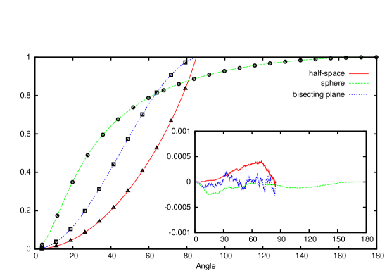
Figure 2: The curves are the predicted cdf’s for the hitting density for the half-space (eq. (2)) and the sphere (eq. (3)) and for the first hit of the bisecting plane (eq. (4)). The circles are the simulation results. The inset shows the differences of the predicted and simulated cdf’s. The distance from the center of the sphere to the starting point of the SAW is $a=3/4$.

To simulate the ensemble of SAW’s in the half space $z<1$ that start at the origin and end anywhere on the plane $z=1$, we use the ensemble of $N$-step SAW’s starting at the origin that stay in the half-space $z>0$. For any such SAW we can dilate it and translate it to produce a SAW in the half-space $z<1$ that goes between the origin and the plane $z=1$. We argue in Kennedy_3d_long that if we weight these SAW’s by $||\omega(N)||^{-(\gamma-\rho)/\nu}$, then in the scaling limit we get the desired ensemble.

Finally, to simulate the ensemble of SAW’s in the sphere of radius $1$ centered at the origin which have one endpoint at $(0,0,a)$ and the other endpoint anywhere on the surface of the sphere, we start with the ensemble of $N$ step SAW’s in the full space that start at the origin. We dilate the walk to to produce a walk with one endpoint at the origin and the other endpoint on the sphere of radius $1$ centered at $(0,0,-a)$. We then condition on the event that this dilated walk lies entirely inside the sphere. As we argue in Kennedy_3d_long , if we weight these walks by a suitable function of $\omega(N)$, then as $N\rightarrow\infty$ we will get the scaling limit of the desired ensemble. In this ensemble there are lattice effects that come from the orientation of the surface of the sphere with respect to the lattice. They persist in the scaling limit and must be taken into consideration when we test our prediction for the hitting density Kennedy_3d_long .

We simulate all three of these ensembles with $N=10^{6}$ and generate on the order of $100$ million samples. The simulation of the SAW in the sphere took a little more than $100$ CPU-days. The other two simulation were much faster, taking on the order of $100$ CPU-hours. When the SAW $\omega$ ends close to where it starts, $||\omega(N)||$ will be relatively small. Such SAW’s are improbable, but the weighting factor is large, and so the statistical errors in the simulation are increased. Such walks are excluded from the ensemble of SAW’s in the sphere, but are a problem in the other two ensembles. The troublesome SAW’s typically have a value of $\theta$ near $90$. So if we condition the random variable $\theta$ on $\theta\leq\theta_{0}$ with $\theta_{0}$ less than $90$, we can reduce this problem. We take $\theta_{0}=85$.

The results of our simulations testing these predictions are shown in figure 2. For the SAW in the sphere we take the distance from the center to the starting point of the SAW to be $a=3/4$. For all three of the predictions we study the cumulative distribution function (cdf) of the random variable $\theta$. In the main figure the three curves are the predictions for the cdf’s and the points give the simulation results at selected values of $\theta$. They are indistinguishable in this figure. The differences of the simulation cdf’s and the predicted cdf’s are shown in the inset. Note the scale of the vertical axis. The differences are on the order of a few hundredths of a per cent, thus providing strong evidence that the SAW is conformally invariant in three dimensions.

Acknowledgements: The support of the Mathematical Sciences Research Institute where this research was begun is gratefully acknowledged.

References

- (1) G. F. Lawler, O. Schramm, and W. Werner, in Fractal geometry and applications: a jubilee of Benoît Mandelbrot, Part 2, Proc. Sympos. Pure Math., Vol. 72 (Amer. Math. Soc., Providence, RI, 2004) pp. 339–364
- (2) T. Kennedy, Phys. Rev. Lett. 88, 130601 (2002)
- (3) T. Kennedy, J. Stat. Phys. 114, 51 (2004)
- (4) T. Kennedy and G. Lawler, Arxiv preprint arXiv:1109.3091(2011)
- (5) J. Cardy, Nuc. Phys. B 240, 514 (1984)
- (6) J. Cardy and S. Redner, Journal of Physics A: Mathematical and General 17, L933 (1984)
- (7) T. Hara and G. Slade, Commun. Math. Phys. 147, 101 (1992)
- (8) T. Hara and G. Slade, Rev. Math. Phys. 4, 235 (1992)
- (9) D. Brydges and G. Slade, Proceedings of the International Congress of Mathematicians (ed. R. Bhatia et al.) 4, 2232 (2010)
- (10) J. Des Cloizeaux and G. Jannink, Polymers in solution: their modelling and structure, Vol. 4 (Clarendon Press Oxford, 1990)
- (11) E. Eisenriegler, Polymers near surfaces: conformation properties and relation to critical phenomena (World Scientific, 1993)
- (12) P. Flory, J. Chem. Phys. 17, 303 (1949)
- (13) B. Nienhuis, Phys. Rev. Lett. 49, 1062 (1982)
- (14) N. Clisby, Phy. Rev. Lett. 104, 55702 (2010)
- (15) R. D. Schram, G. T. Barkema, and R. H. Bisseling, Journal of Statistical Mechanics: Theory and Experiment 2011, P06019 (2011)
- (16) R. Hegger and P. Grassberger, J. Phys. A 27, 4069 (1994)
- (17) N. Clisby, J. Stat. Phys. 140, 349 (2010)
- (18) T. Kennedy, J. Math. Phys. 53, 095219 (2012)
- (19) T. Kennedy, “Monte Carlo tests of conformal invariance predictions for the 3D self-avoiding walk,” (preprint)