Switching exciton pulses through conical intersections

Abstract

Exciton pulses transport excitation and entanglement adiabatically through Rydberg aggregates, assemblies of highly excited light atoms, which are set into directed motion by resonant dipole-dipole interaction. Here, we demonstrate the coherent splitting of such pulses as well as the spatial segregation of electronic excitation and atomic motion. Both mechanisms exploit local non-adiabatic effects at a conical intersection, turning them from a decoherence source into an asset. The intersection provides a sensitive knob controlling the propagation direction and coherence properties of exciton pulses. The fundamental ideas discussed here have general implications for excitons on a dynamic network.

Introduction: Frenckel Excitons Frenkel (1931), in which excitation energy of an interacting quantum system is coherently shared among several constituents, are a fundamental ingredient of photosynthetic light harvesting May and Kühn (2001). Recently, they have become accessible in ultracold Rydberg gases, due to strong long-range dipole-dipole interactions Park et al. (2011a, b); Li et al. (2005); Westermann et al. (2006); Mülken et al. (2007); Bettelli et al. (2013); Günter et al. (2013); Ravets et al. (2014); Barredo et al. (2014) and large lifetimes of atomic Rydberg states Gallagher (1994); Beterov et al. (2009). Assemblies of several regularly placed and Rydberg excited cold atoms – flexible Rydberg aggregates – provide new concepts such as adiabatic guiding of an exciton through atomic chains as an exciton pulse Ates et al. (2008); Wüster et al. (2010); Möbius et al. (2011). Such a pulse is initiated by a displacement of one atom in the regular chain. The displacement simultaneously localizes the exciton on the atom pair with the smallest separation and initiates the pulse, i.e., the motion of the exciton. Subsequent binary collisions propagate the exciton pulse and the associated entanglement through the chain with very high fidelity. Without atomic motion this would require careful tuning of interactions Asadian et al. (2010); Eisfeld (2011); Saikin et al. (2013); Kühn and Lochbrunner (2011).

That this propagation along a one-dimensional (1D) chain of atoms preserves the exciton with high fidelity Wüster et al. (2010) is remarkable, since the transport appears quite fragile requiring a lossless locking in of electronic excitation transfer and atomic motion. However exciton transport often occurs in higher dimensional systems, where it is a priori unclear if we can also guide and control the exciton pulse. Already a two-dimensional setup of atoms gives rise to conical intersections (CIs) Carrington (1974); Mead and Truhlar (1979); Wüster et al. (2011) which might compromise adiabaticity known to be an important prerequisite of exciton transport. On the other hand CIs can play constructive roles in photochemical processes Domcke et al. (2004), hence might be similarly useful for atomic aggregates.

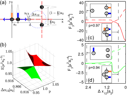
Figure 1: (color online) (a) Orthogonal atom chains with one Rydberg dimer each. Atoms 0 and 1 initially share an excitation, due to which atom 1 reaches the conical intersection at ${x}_{\mbox{\!\! \scriptsize CI}}$. The origin of the coordinate system is set to the mean initial position of atom 0. (b) The repulsive energy surface $U_{\mathrm{rep}}$ (red) and middle surface $U_{\mathrm{mid}}$ (green) of the trimer sub-unit (atom 1, 2 and 3) near the CI. (c,d) Forces on atom 2 (solid lines) and atom 3 (dashed lines), for the repulsive surface (red,c) and middle surface (green,d). The insets show atomic positions and the excitation distribution ($d_{n}$, see text) of exciton states and forces for the indicated values of $\Delta x_{12}$, which denotes the distance between atom 1 and the vertical chain. The parameter $p$ controls the degree of symmetry of the trimer, where $p=1$ corresponds to an isosceles trimer configuration.

In the following, we will show how an exciton pulse can be coherently split through a CI that arises between two excitonic Born-Oppenheimer (BO) surfaces of the system. The junction between two atomic chains that gives rise to the conical intersection can be functionalized in two ways, as a beam-splitter or a switch, sending the pulse split in both directions on the second chain or in only the one preselected. The surfaces involved in the CI serve as output modes of the beam-splitter. We will explicitly demonstrate that the junction constitutes a sensitive point where essential characteristics of the exciton pulse propagation can be controlled through small shifts in external trapping parameters. Our results concern exciton transport on any network whose constituents move, such as (artificial) light-harvesting devices Saikin et al. (2013).

T-shaped aggregates: The junction is created with two chains of Rydberg atoms in a T-shape configuration (FIG. 1a), with the required one-dimensional confinement generated optically Li et al. (2013); Mukherjee et al. (2011). Specifically, we will use $2N$ Rydberg atoms with mass $M=11000$ a.u. and principal quantum number $\nu=44$. We assume that $N$ of these atoms are constrained on the $x$-axis, and the other $N$ on the $y$-axis, such that all atoms can only move freely in one dimension. We start with one Rydberg atom in an angular momentum $p$-state, while the rest are in $s$-states. The electronic wavefunction $|\,{\psi_{\rm{el}}({\mathbf{R}})}\,\rangle$ of the whole system can be expanded in the single excitation basis $|\,{\psi_{\rm{el}}({\mathbf{R}})}\,\rangle=\sum_{n=1}^{2N}c_{n}(t)|\,{\pi_{n}}\,\rangle,$ where $|\,{\pi_{n}}\,\rangle=|\,{s\dots p\dots s}\,\rangle$ is the state with the $n$-th atom in the $p$-state Ates et al. (2008); Wüster et al. (2010); Möbius et al. (2011) and ${\mathbf{R}}~{}=~{}({\mathbf{R}}_{1},\dots,{\mathbf{R}}_{2N})^{\rm{T}}$ groups all atomic coordinates ${\mathbf{R}}_{n}$. The system is ruled by the Hamiltonian

$$\hat{H}=-\frac{\hbar^{2}}{2M}\nabla^{2}_{{\mathbf{R}}}+\sum_{m\neq n=1}^{2N}\left(\hat{V}_{\rm{dd}}(R_{mn})+\hat{V}_{\rm{VDW}}(R_{mn})\right)\,,$$ (1)

where $R_{mn}=|{\mathbf{R}}_{m}-{\mathbf{R}}_{n}|$ is the distance between atoms $m$ and $n$.

The long-range Rydberg-Rydberg interactions Gallagher (1994) are described with two explicit contributions $\hat{V}_{\mathrm{dd}}$ and $\hat{V}_{\mathrm{VDW}}$, a resonant dipole-dipole and a van der Waals term, respectively. $\hat{V}_{\mathrm{dd}}$ couples excitations $|\,{\pi_{n}}\,\rangle$ on different atoms $n$ through

$$\hat{V}_{\rm{dd}}(R_{mn})=-\frac{\mu^{2}}{R_{mn}^{3}}|\,{\pi_{m}}\,\rangle\langle\,{\pi_{n}}\,|\,,$$ (2)

where $\mu=d_{\nu,1;\nu,0}/\sqrt{6}$ is the scaled radial matrix element. The non-resonant van der Waals (VDW) interaction

$$\hat{V}_{\rm{VDW}}(R_{mn})=-\frac{C_{6}}{2R_{mn}^{6}}\mathbb{I}\,,$$ (3)

ensures for $C_{6}<0$ repulsive behavior at very short distances regardless of the electronic state. Therefore, $\mathbb{I}$ denotes a unit matrix in the electronic space. We sketch in sup how this simple model of interactions arises from the full molecular physics of interacting Rydberg atoms Goy et al. (1986) using a magnetic field and selected total angular momentum states.

As previously shown Ates et al. (2008); Wüster et al. (2010, 2011); Möbius et al. (2011), the joint motional and quantum state dynamics can be well understood from the eigenstates $|\,{\varphi_{k}({\mathbf{R}})}\,\rangle$ of the electronic Hamiltonian ${\hat{H}}_{\mbox{\!\! \scriptsize el}}({\mathbf{R}})=\sum_{m\neq n}[\hat{V}_{\rm{dd}}+\hat{V}_{\rm{VDW}}]$. These eigenstates and the corresponding eigenenergies $U_{k}({\mathbf{R}})$ depend parametrically on ${\mathbf{R}}$ and are referred to as Frenkel excitons Frenkel (1931) and Born-Oppenheimer surfaces (BO surfaces), respectively. The total wavefunction including atomic motion can be written as $|\,{\Psi(\mathbf{R})}\,\rangle=\sum_{n}\phi_{n}({\mathbf{R}})|\,{\varphi_{n}({\mathbf{R}})}\,\rangle$. To solve the coupled electronic and motional dynamics, we employ Tully’s fewest switching algorithm Tully and Preston (1971); Hammes-Schiffer and Tully (1994); Barbatti (2011); Jasper and Truhlar (2005); sup , a quantum-classical method that is well established for our type of problem Wüster et al. (2010); Möbius et al. (2011, 2013).

Two perpendicular dimers: To realize a T-shape chain, a minimum of two dimers is required, see FIG. 1a. The atoms have a Gaussian distribution about their initial location ${\mathbf{R}}_{0}$ along their chain with width $\sigma=0.5\ \mathrm{\mu m}$ as sketched. Transverse to the chain we assume perfect localization. The bars in FIG. 1a visualize the excitation amplitude of the exciton on the repulsive BO surface $|\,{\varphi_{\mathrm{rep}}({\mathbf{R}}_{0})}\,\rangle$. For each atom the length of the bar shows $d_{n}=\mbox{$\langle\,{\pi_{n}}\,|\,{\varphi_{\mathrm{rep}}({\mathbf{R}}_{0})}\,\rangle$}$, orange for positive and blue for negative values. As one can see, initially the single p-excitation in the system is shared among atom 0 and 1. On the BO-surface $k$, the force on atom $n$ is given by $\mathbf{F}_{nk}=-\nabla_{\mathbf{R}_{n}}U_{k}({\mathbf{R}})$. Due to the initial repulsive force ${F}_{\mbox{\!\! \scriptsize n,rep}}$ (blue arrows) atom 1 moves and eventually reaches the position $x_{\mathrm{CI}}$, where the atoms 1-3 form a planar trimer. The two highest BO surfaces of this trimer conically intersect when the three atoms form an equilateral triangle, as shown in FIG. 1b and studied in detail in Wüster et al. (2011). In the following we will call these surfaces the repulsive (red) and middle (green) surface, respectively.

Exciton splitting: Initialized on the repulsive surface of the global (double dimer) system, the exciton pulse is transferred to the vertical chain via the conical intersection onto these two electronic surfaces – the repulsive and the middle one – dependent on the position of atom 1 relative to atom 2 and 3 in the y-direction when it enters the trimer configuration (see parameter $p$ in FIG. 1a). Viewed from the perspective of the trimer subsystem only, the exciton pulse enters on the middle surface, where the excitation amplitude (blue bar) matches the initial excitation distribution, see insets of FIG. 1c,d. If atom 1 arrives right in the middle between atoms 2 and 3, the atomic trimer passes through the degenerate point of the CI leading to significant transfer of exciton amplitude to the repulsive surface (FIG. 1c). If this is not the case, an asymmetric trimer configuration is realized for which non-adiabatic transitions due to the CI are much weaker and the system remains on the middle trimer surface leading to the situation of FIG. 1d with quite different forces on atom 2 and 3. This has profound consequences on the atomic motion: Amplitude on the repulsive surface leads to a symmetric repulsion of atoms 2 and 3 of the vertical chain, creating the outer pulses in the density shown in FIG. 2b. A representative quantum-classical trajectory is shown as white dotted line, with $p=0.98$. On the repulsive surface atom 1 is often reflected off the vertical chain as visible in FIG. 2a. On the other hand, amplitude on the middle surface has the effect of a very asymmetric atomic motion in y, with that atom on the y-axis remaining almost at rest which has initially the smaller distance to the location of the dimer on the x-axis. This type of motion is responsible for the inner and central features in FIG. 2b, with a representative trajectory shown white dashed with $p=0.82$. One can also recognize the variant of the motion, where the other vertical atom remains at rest. The middle surface is mainly responsible for atom 1 freely passing the vertical chain in FIG. 2a.

Since the nuclear wave packet of the exciton pulse will have a distribution of positions of atoms 1, 2 and 3, there will be in general a splitting of the exciton when it has passed the conical intersection with the electronic excitation propagating on the repulsive as well as the middle surface. In fact, about 50% of the initial amplitude has been transferred from the middle to the repulsive surface after $3\ {\mu}$s under the initial conditions for our exciton pulse leading to the dynamics of FIG. 2.

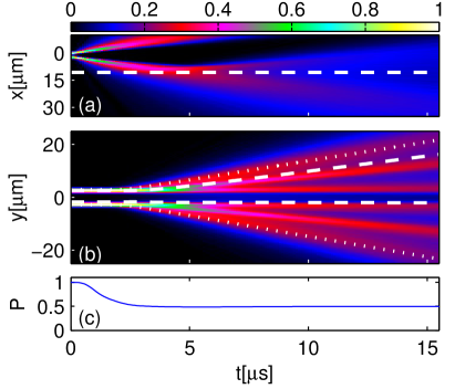
Figure 2: (color online) Normalized total atomic density for atomic motion on two BO surfaces; overlayed are selected trajectories of the quantum classical method. (a) horizontal density $n(x,t)$ (see sup ) of atom 0 and 1. The dashed white line marks the x-position of the vertical chain. (b) vertical density $n(y,t)$ of atom 2 and 3. In (a,b) we actually plot $\sqrt{n(x,t)}$, $\sqrt{n(y,t)}$. (c) Purity of reduced electronic state, see sup . Our calculations are for lithium atoms excited to principal quantum number $\nu=44$ with a transition dipole moment of $\mu=1000$ a.u.. The parameters of the initial atomic configuration were $a_{1}=2.16\ \rm{\mu m}$, $a_{2}=5.25\ \rm{\mu m}$ and $d=8.5\ \rm{\mu m}$. To sample the nuclear wavefunction, we have propagated $10^{5}$ trajectories Dennis et al. (2013) with a standard deviation of $\sigma_{x}=0.5\ \rm{\mu m}$ for the atomic positions. Here, we have used $C_{6}=0$ for simplicity.

Hence, not only does the exciton split into two parts traveling with the atoms in opposite directions in the y-chain, we have a further coherent splitting of electronic excitation into the middle and repulsive electronic surface: The total initial wave function was $|\,{{\Psi}_{\mbox{\!\! \scriptsize ini}}(\mathbf{R})}\,\rangle={\phi}_{\mbox{\!\! \scriptsize 0}}({\mathbf{R}})|\,{{\varphi}_{\mbox{\!\! \scriptsize rep}}({\mathbf{R}})}\,\rangle$, where ${\phi}_{\mbox{\!\! \scriptsize 0}}({\mathbf{R}})$ describes the initial, harmonically trapped, spatial ground state. After the evolution shown in FIG. 2, the wave function reads $|\,{{\Psi}_{\mbox{\!\! \scriptsize fin}}(\mathbf{R})}\,\rangle={\phi}_{\mbox{\!\! \scriptsize rep}}({\mathbf{R}})|\,{{\varphi}_{\mbox{\!\! \scriptsize rep}}({\mathbf{R}})}\,\rangle+{\phi}_{\mbox{\!\! \scriptsize mid}}({\mathbf{R}})|\,{{\varphi}_{\mbox{\!\! \scriptsize mid}}({\mathbf{R}})}\,\rangle$.

In this final state $|\,{{\Psi}_{\mbox{\!\! \scriptsize fin}}(\mathbf{R})}\,\rangle$ the atomic configuration and the electronic state are entangled, which can be quantified through the purity of the reduced electronic density matrix. It is obtained by averaging over the atomic position as described in sup ; Wüster et al. (2010); Möbius et al. (2011). The purity drops from one to $1/2$ when the exciton is split, as shown in FIG. 2d, reflecting a transition from a pure to a mixed state. For the total (pure) system state, this implies a transition from a separable to an entangled state.

Exciton switch: The minimal T-shape system consisting of two dimers discussed so far primarily serves the purpose to elucidate the central element for exciton pulse control, namely the junction between perpendicular atomic chains. Ultimately, we would like to interface the two dimers in FIG. 1a with longer atomic chains that can support exciton pulses as described in Wüster et al. (2010). Such a pulse travels to the junction to become coherently split as just described, with the resulting exciton pulses on the vertical chain depending on how the conical intersection of the trimer at the junction was passed. Since the relative strength of the exciton pulse on the middle and repulsive surface of the trimer depends on the atomic positions and momenta near the conical intersection, we can control the exciton pulse propagation on the vertical chain, for example via the position of the horizontal chain relative to the vertical one. We demonstrate this effect with 3 atoms on the horizontal and 4 atoms on the vertical chain, allowing for a vertical offset $\Delta y$ of the horizontal chain from the center of the vertical chain, and a variable separation $a_{2}$ of the two central atoms in the second chain, see sketch in FIG. 4.

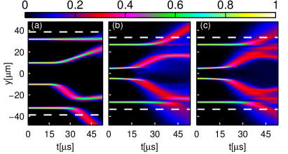
Figure 3: (color online) Use of the trimer subunit with conical intersection as an exciton switch. Depending on the geometry, we can realize three qualitatively different scenarios: (a) asymmetric, repulsive surface; (b) asymmetric, middle surface; (c) symmetric, repulsive and middle surface. Each plot shows $\sqrt{n(y,t)}$ as in FIG. 2. When atoms reach the white horizontal lines (${r}_{\mbox{\!\! \scriptsize coll}}$, $6.6\mu$m beyond the initial $y$-position of atoms 3, 6), we extract the level of bi-partite entanglement, listed in FIG. 4. The parameters different to those of FIG. 2 are $\nu=80$ (hence $\mu=3374$ a.u.), $a_{1}={6}{\mu}$m, $d={22}{\mu}$m and $C_{6}\approx{-7.6\cdot 10^{20}}$ a.u. as derived in sup . Also see sup for videos of representative single trajectories.

With small variations of the two parameters $\Delta y$, $a_{2}$, qualitatively very different scenarios can be realized as illustrated with FIG. 3 and FIG. 4.

In scenario (a), the spacing $a_{2}$ and the shift $\Delta y$ are so large that the trimer subunit discussed before does not form foo . Since atom $2$ approaches $4$ closest (see FIG. 4), the exciton-pulse travels in the downwards direction. To switch it upwards we would use $\Delta y\rightarrow-\Delta y$. We characterize the relevant entanglement transport using $\bar{E}_{ij}$, the bi-partite entanglement Hill and Wootters (1997); Wootters (1998); sup ; Wüster et al. (2010); Möbius et al. (2011) during the last collision of the two terminal atoms $i,j$ on the vertical chain, i.e., $(i,j)=(5,6)$ upwards and $(i,j)=(3,4)$ downwards. We know the last collision is in progress, whenever atom $3$ (atom $6$) reaches position ${r}_{\mbox{\!\! \scriptsize coll}}$, indicated in FIG. 3 by horizontal white lines for the downwards (upwards) direction. Our results in FIG. 4 reveal that pulse propagation is linked with high fidelity entanglement transport, demonstrating successful control of the direction of exciton-pulse propagation without loosing coherence.

In scenario (b) we segregate mechanical and electronic degrees of freedom of the exciton-pulse, by choosing $a_{2}$ small enough such that a trimer subunit forms at the junction. Since an offset $\Delta y$ is kept, the nuclear wave packet, however, misses the conical intersection and remains on the middle trimer surface. Importantly, the middle trimer surface does not connect to a global surface allowing coherent exciton pulse transport: At the first collision within the vertical chain (between atoms $3$ and $4$ in FIG. 3b), part of the excitation evades those atoms and delocalizes on the remnant upper chain. Momentum is henceforth transported downwards by van der Waals collisions only such that the original exciton pulse with entangled atom and electron dynamics has been ripped apart. For this momentum transport without excitation transport, the inclusion of VDW interactions is crucial. They further cause the atom on the y-axis closest to the x-axis to carry most acceleration, in contrast to FIG. 2.

Finally, in scenario (c) $\Delta y=0$ and the wave packet fully traverses the conical intersection at the junction. Here, the trimer subunit operates as described in the first part of the article. The wave packet is split onto both, the repulsive and middle trimer surface. As discussed for scenario (b), the middle trimer surface does not give rise to exciton-pulse propagation. On the repulsive surface, one gets symmetric (up-down) propagation of two pulses as expected. However, the entanglement transport in both directions is much weaker than in scenario (a) which is due to the fact that the atoms still share only a single p-excitation. Subsequent non-adiabatic effects allow a strong coherent pulse only in a single direction. Even within this symmetric scenario, the relative importance of the middle and repulsive surface can be tuned via the effective size of the conical intersection Teller (1937), determined by atomic velocities and separation (energy splittings).

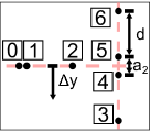
.scenario (a) (b) (c) $a_{2}$ ${20}\mu$m ${9.5}\mu$m ${9.5}\mu$m ${\Delta}y$ ${1.5}\mu$m ${1.5}\mu$m 0 up, $\Big{.}\bar{E}_{56}$ $0\%$ ${60}\%$ ${24}\%$ down, $\Big{.}\bar{E}_{34}$ ${97}\%$ ${7}\%$ ${24}\%$

Figure 4: Geometry and entanglement switching for the three scenarios of FIG. 3. Atom numbering and control parameters $a_{2}$, ${\Delta}y$ are defined in the sketch on the left. The entanglement measure $\bar{E}_{ij}$ is defined in sup .

Conclusions: We have shown how an exciton pulse can be coherently split through non-adiabatic dynamics at a conical intersection in a flexible Rydberg aggregate. Our results turn a junction between two Rydberg atom chains into a switch. The switch can control if and how exciton pulses continue to propagate in the system. Similar physics may be of interest for research on artificial light harvesting systems McConnell et al. (2010), where exciton transport and control is quintessential for energy efficiency. The atomic junction introduced here also provides a tool to directly examine the many-body dynamics near conical intersections in the laboratory.

The exciton splitting predicted could be experimentally monitored using high resolution Rydberg atom detection schemes Schwarzkopf et al. (2011); Olmos et al. (2011); Günter et al. (2012) which are in addition state selective. Applied to our system, they allow a direct visualization of many-body wave packet dynamics near a conical intersection. The essential modular subunit of an atomic trimer exhibiting a CI can be envisaged as a building block for networks of exciton carrying atomic chains or a device for controlling the energy flow in molecular aggregates.

$${\mathbf{d}}_{mn}({\mathbf{R}})=\langle\,{\varphi_{m}({\mathbf{R}})}\,|\nabla_{{\mathbf{R}}}|\,{\varphi_{n}({\mathbf{R}})}\,\rangle.$$ (4)

The sequence of propagation is as follows: The positions and velocities of the atoms are randomly determined. The electronic Hamiltonian is diagonalized and we use one eigenenergy $U_{k}$ of our choice as potential for the atoms. The atoms are propagated one time step via Newton’s equation

$$M\ddot{{\mathbf{R}}}=-\nabla_{{\mathbf{R}}}U_{k}({\mathbf{R}}).$$ (5)

The new positions lead to new eigenstates and -energies and to new diabatic and adiabatic coefficients. We propagate the diabatic coefficients via

$$\mathrm{i}\hbar\dot{c}_{k}(t)=-\mu^{2}\sum_{l\neq k}^{2N}\frac{c_{l}(t)}{|{\mathbf{R}}_{k}-{\mathbf{R}}_{l}|^{3}}$$ (6)

To close the loop, the nuclei will be propagated via (5) again.
We imagine the atoms were confined in individual harmonic traps, before these are released to let all atoms move. This motivates Gaussian probability distributions of the atomic positions and momenta. We label the standard deviation in position of atoms on chain $i$ by $\sigma_{x_{i}}$. The velocity probability distribution then has a standard deviation $\sigma_{v_{i}}=\hbar/(M\sigma_{x_{i}})$.

Validation:

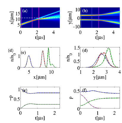
Figure 5: Comparison of Tully’s surface hopping with full quantum mechanical calculations, for exciton switch similar to Fig. 2 of the main article. (a) Horizontal density $\sqrt{n(x,t)}$ of atom 1 from Tully’s method. Vertical lines indicate snap shots shown in panel (c). The dashed white line marks the location of the vertical chain. (c) Horizontal density $n(x,t_{k})$ of atom 1 from Schrödinger equation (solid) and Tully’s surface hopping (black dashed). (blue) $t_{1}=0$, (red) $t_{2}=1.4\mu$s, (green) $t_{3}=2.2\mu$s. (b,d) The same for the density on the vertical chain $\sqrt{n(y,t)}$, $n(y,t_{k})$ of atom 2 and 3. (e) Population on Born-Oppenheimer surfaces (color) quantum, (black-dashed) Tully. (f) Excitation probability on each atom, quantum: (magenta) atom 0, (blue) atom 1, (green) atoms 2 and 3, (black-dashed) Tully.

Tully’s fewest switching algorithm discussed above has already been benchmarked successfully for exciton dynamics on Rydberg chains in Wüster et al. (2010); Möbius et al. (2011, 2013). For the exciton switch discussed here, an essential new ingredient is the conical intersection resulting in strong non-adiabatic effects. We show here that these are captured by Tully’s method very well, by comparison with full quantum-mechanical calculations. To make the strongest connection with the present work, we study a scenario close to the exciton switch shown in Fig. 2.

Modifications that were necessary to keep quantum simulations tractable are a freezing of the motion of atom 0, and the removal of its position uncertainty. Further the initial acceleration period is removed, instead atom 1 is shifted by ${x}_{\mbox{\!\! \scriptsize shift}}=2.5\mu$m towards positive $x$ and given an initial mean velocity ${v}_{\mbox{\!\! \scriptsize shift}}=2.5$m/s. This is about half of what would correspond more closely to Fig. 2, however larger velocities would require too fine numerical grids. As described in [19], we then solve a multi-component Schrödinger equation in the electronic $|\,{\pi_{n}}\,\rangle$ basis.

As seen in FIG. 5, both exciton- and spatial dynamics are captured satisfactorily by the quantum-classical method. The performance of Tully’s method has been intensively studied in the context of quantum chemistry (e.g. [27]). For the dynamics of exciton transport on moving (flexible) Rydberg assemblies studied here, the present comparison and that of Ref. Wüster et al. (2010) shows excellent agreement. A distinguishing feature of our systems is that spatial interferences on any BO surface typically do not occur, thus spatial coherence information that is not included in Tully’s method is not required.

The trimer: “Trimer” refers to an assembly of three Rydberg atoms. Since main features of the systems we studied can be understood by considering only three atoms, we provide here full details in addition to the features discussed in the main text.

Figure 6: Sketch of a trimer near a configuration with CI. Atom 1 is confined on a horizontal line and atom 2 and 3 on a vertical line. The parameter $p$ adjusts the distance of atom 2 and 3 from the horizontal line and for $p\neq 1$ results in nonequilateral triangle configurations. All distances are expressed in units of $\mathrm{u}$, the distance between atom 2 and 3.

The configurations of the trimer which are most relevant here are shown in FIG. 6. We call the overall length scale $\mathrm{u}$. The geometry of the trimer around the equilateral triangle configuration is described by the distance $x$ between atom 1 and the other two atoms and the parameter

$$p:=2\frac{|\langle{\mathbf{R}}_{2},{\mathbf{e}}_{y}\rangle|}{|{\mathbf{R}}_{2}-{\mathbf{R}}_{3}|},$$ (7)

which we call the asymmetry parameter, since it controls the degree of symmetry with respect to the isosceles triangle. The biggest and smallest eigenenergy are globally repulsive or attractive, respectively Ates et al. (2008); Wüster et al. (2011). We label them $U_{\rm{rep}}$ and $U_{\rm{att}}$ and the corresponding eigenstates $|\,{\varphi_{\rm{rep}}}\,\rangle$ and $|\,{\varphi_{\rm{att}}}\,\rangle$. We call these repulsive and attractive surface and eigenstate, respectively. There is another eigenenergy energetically between them. We label it $U_{\rm{mid}}$ and the corresponding eigenstates $|\,{\varphi_{\rm{mid}}}\,\rangle$. We call it middle surface and eigenstate.

Symmetric case $p=1$.

The middle and repulsive eigenenergies have the value $\mu^{2}\mathrm{u}^{-3}$, when they cross. This happens, when $x=x_{CI}:=\sqrt{3}/2\ \mathrm{u}$, i.e. at the equilateral triangle configuration. It is well known that this is a conical intersection Wüster et al. (2011); Carrington (1974); Mead and Truhlar (1979). FIG. 7 (a) shows the eigenergies as a function of the horizontal distance $x$. The middle eigenenergy stays constant for $x<x_{CI}$ as it arises solely from the interaction energy of atom 2 and 3. When atom 1 is far away from the other two, the middle and attractive energies are vanishing, whereas when the system realizes a linear trimer ($x=0$), the repulsive and attractive energy values are extremal.

Asymmetric case $p\neq 1$.

There is no crossing of eigenvalues for $p\neq 1$. FIG. 7 (b) shows the energy separation between the repulsive and the middle state over the horizontal distance $x$ of the atoms for different asymmetry parameters $p$. With increasing asymmetry, the smallest energy splitting increases, as does the value of $x$ where the splitting is smallest. From now on we call atomic configurations asymmetric, when they correspond to values of $p\ll 1$ and symmetric, when $p\approx 1$.

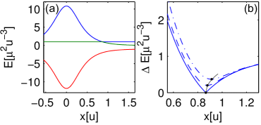
Figure 7: Eigenenergy spectra for the trimer. (a) Eigenenergies over horizontal distance x for the symmetric case $p=1$. The repulsive (blue line) and middle eigenenergy (green line) cross at x=$\sqrt{3}/2\ \mathrm{u}$. (b) Energy spacing between repulsive and middle eigenenergy for different asymmetry parameters, $p=1$ (solid), $p=0.88$ (dashed), $p=0.76$ (dashed dotted). The minimal energy spacing (black dots) is shifted to bigger $x$ for higher asymmetry, which is well described by the analytical result Eq. (12) (grey line).

Using the parameters just defined, we can analyse the forces on the atoms for the two relevant BO-surfaces and find characteristically different behaviour as shown in Fig. 1 of the main article and discussed therein.

For the trimer, it is well known that where the atoms build an equilateral triangle, the energy surfaces exhibit a CI. We now analyze the eigenenergies and eigenstates near the CI in order to understand the numerical results in FIG. 7. All different geometries of the trimer around the conical intersection can be described by the two parameters $\Delta x:=x-x_{CI}$ and $p$, illlustrated in FIG. 6. We collect both in the vector ${\mathbf{\chi}}~{}:=~{}[\Delta x,p]^{\rm{T}}$. The equilateral triangle configuration corresponds to ${\mathbf{\chi}}_{0}~{}:=~{}[0,1]^{\rm{T}}$, with the degenerate eigenvalue $E^{(0)}_{CI}~{}=~{}\mu^{2}/\mathrm{u}^{3}$. The corresponding eigenstates can be $|\,{\varphi^{(0)}_{CI,1}}\,\rangle~{}=~{}\frac{1}{\sqrt{2}}\begin{bmatrix}-1&0&1\end{bmatrix}^{\rm{T}}$ and $|\,{\varphi^{(0)}_{CI,2}}\,\rangle~{}=~{}\frac{1}{\sqrt{6}}\begin{bmatrix}-1&2&-1\end{bmatrix}^{\rm{T}}$. The electronic Hamiltonian of the Configuration shown in FIG. 6 is given by

$$\hat{H}_{\rm{el}}({\mathbf{\chi}})=-\mu^{2}\begin{bmatrix}0&s_{1}^{-3}({\mathbf{\chi}})&s_{2}^{-3}({\mathbf{\chi}})\\ s_{1}^{-3}({\mathbf{\chi}})&0&s_{3}^{-3}\\ s_{2}^{-3}({\mathbf{\chi}})&s_{3}^{-3}&0\\ \end{bmatrix}.$$ (8)

We use degenerate perturbation theory to estimate the energy gap near the CI. To do so we first Taylor expand the electronic Hamiltonian around the CI configuration up to second order in ${\mathbf{\chi}}$:

$$\hat{H}^{\rm{as}}_{\rm{el}}({\mathbf{\chi}})\approx\hat{H}^{\rm{CI}}_{\rm{el}}+\hat{H}^{\rm{PT}}_{\rm{el}}({\mathbf{\chi}}),$$ (9)

where $\hat{H}^{\rm{CI}}_{\rm{el}}$ is the electronic Hamiltonian at the CI configuration and $\hat{H}^{\rm{PT}}_{\rm{el}}({\mathbf{\chi}})$ is the perturbation. We define the perturbation matrix

$$S_{\rm{el}}({\mathbf{\chi}})_{\alpha\beta}:=\langle\,{\varphi^{(0)}_{CI,\alpha}}\,|\hat{H}^{\rm{PT}}_{\rm{el}}({\mathbf{\chi}})|\,{\varphi^{(0)}_{CI,\beta}}\,\rangle.$$ (10)

The eigenenergies $E^{\rm(1)}_{1}({\mathbf{\chi}}),E^{\rm(1)}_{2}({\mathbf{\chi}})$ of $S_{\rm{el}}({\mathbf{\chi}})$ are the first order corrections to the energy and lift the degeneracy. Thus the energy gap is given by $\Delta E^{\rm{as}}({\mathbf{\chi}})~{}=~{}|E^{\rm(1)}_{1}({\mathbf{\chi}})-E^{\rm(1)}_{2}({\mathbf{\chi}})|$ to first order. Consistently expanding this expression to second order around ${\mathbf{\chi}}_{0}$, we get

$$\dfrac{\Delta E^{\rm{as}}({\mathbf{\chi}})}{\mu^{2}}\approx\sqrt{12\Delta x^{2}+(1-p)^{2}\biggl{(}3-\frac{31\sqrt{3}\Delta x}{2}+\frac{1061\Delta x^{2}}{8}\biggr{)}}$$ (11)

for $p\lesssim 1$. The asymmetry of the configuration is measured by $1-p$. For every small given asymmetry, there is a $\Delta x_{\rm{min}}$ where the energy gap becomes minimal:

$$\begin{split}\Delta x_{\rm{min}}&\approx 1.12\cdot(1-p)^{2}\\ \Delta E^{\rm{as}}_{\rm{min}}(p)&\approx\sqrt{3}\cdot(1-p)\end{split}$$ (12)

Thus the horizontal distance between atom 1 and the other atoms has to be bigger compared to the CI configuration, to achieve a minimal energy gap as evident in FIG. 7.

Entanglement measure: As described in more detail, the quantum mechanical electronic density matrix $\hat{\sigma}=\sum_{n,m}\sigma_{nm}|\,{\pi_{n}}\,\rangle\langle\,{\pi_{m}}\,|$ is represented by

$$\sigma_{nm} =\overline{c_{n}^{*}c_{m}},$$ (13)

in a quantum-classical framework, where $\overline{\cdots}$ denotes the trajectory average. The purity $P=\mbox{Tr}[\hat{\sigma}^{2}]$ quantifies to which extent the reduced electronic state is mixed ($P=0$) or pure ($P=1$).

We can further obtain a reduced density matrix for just two atoms

$$\hat{\beta}_{ab}={\mbox{Tr}}^{\{a,b\}}\big{[}\hat{\sigma}\big{]}.$$ (14)

by performing the trace ${\mbox{Tr}}^{\{a,b\}}\big{[}\cdots\big{]}$ over the electronic states for all atoms other than $a$, $b$. For a single p-excitation in the system, this takes the form

$$\hat{\beta}_{ab}=\left(\begin{array}[]{cccc}0&0&0&0\\ 0&\sigma_{aa}&\sigma_{ba}&0\\ 0&\sigma_{ab}^{*}&\sigma_{aa}&0\\ 0&0&0&\sum_{c\neq\{a,b\}}\sigma_{cc}\\ \end{array}\right).$$ (19)

The density matrix $\hat{\beta}_{ab}$ may describe mixed versions of entangled states, the entanglement of which is often quantified using $E_{ab}$, the “entanglement of formation” Hill and Wootters (1997); Wootters (1998). It is obtained through the concurrence $C_{ab}=2|\sigma_{ab}|$, with the further definitions $H(x)=-[x\log_{2}x+(1-x)\log_{2}(1-x)]$ and ${\cal E}(x)=H(1/2+\sqrt{1-x^{2}}/2)$ as $E_{ab}={\cal E}(C_{ab})$.

Fig. 4 of the main article then shows the bi-partite entanglement of formation for the two last atoms on the vertical chain, in the respective direction as indicated. Extraction of total atomic density: Fig. 2 and Fig. 3 show the atomic densities on the vertical and horizontal chain. In Tully’s semiclassical method we propagate many individual trajectories with different atom positions, to sample the atomic wavefunction. To obtain total densities, we bin the coordinate of the atoms on the horizontal chain into a discrete grid for the x-axis and for atoms on the vertical chain into a discrete grid for the y-axis. This is averaged over all trajectories. By dividing through the number of atoms per chain $N$, we obtain the normalized total density for each chain. The formula for the x-axis density $n(x,t)$ reads:

$$n(x,t) =\sum\limits_{k=1}^{N_{\mathrm{trajs}}}\sum_{j,m}\Theta\Bigl{(}\frac{\Delta}{2}-|x_{m}-x|\Bigr{)},$$

$$\times\Theta\Bigl{(}\frac{\Delta}{2}-|R^{(k)}_{j,x}(t)-x_{m}|\Bigr{)}/NN_{\mathrm{trajs}},$$ (20)

where $\Theta(x)$ is the Heaviside function, the sum $\sum_{j}$ is over atoms on the horizontal chain only and the sum $\sum_{m}$ over all discrete bins on the x-axis. We used $R^{(k)}_{j,x}(t)$ for the x-coordinate of the $j$’th atom from the $k$’th trajectory and $x_{m}$ for the central bin coordinates. The binning grid spacing is $\Delta$. We now have $\sum_{k=1}^{(R_{f}-R_{i})/\Delta}n(R_{i}+(k+1/2)\Delta,t)=1$, where $R_{i},R_{f}$ are the spatial boundaries of our binning. The definition of the y-axis density $n(y,t)$ is analogous.

Isotropic dipole-dipole interactions: In all simulations we used an electronic basis with a single p-excitation and assumed the dipole-dipole interaction to be isotropic, only dependent on the internuclear distance between two atoms, which we denote here with $R$. If spin-orbit interaction is neglected and the sign of the interaction irrelevant, this situation is achieved by choosing the quantization axis $\hat{z}$ perpendicular to our internuclear distance vectors and considering the magnetic quantum number $m=0$ manifold, which decouples from the others Möbius et al. (2011).

For the simulations of Fig. 2 the principal quantum number was $\nu=44$, which yields a finestructure-splitting of $\Delta E_{\mathrm{FS}}=0.92$ MHz Goy et al. (1986). The characteristic strength of the dipole-dipole interaction $V_{dd}=d_{\mathrm{rad}}^{2}(44)/R^{3}~{}=~{}613$ MHz depends on the distance between the atoms and the radial matrix element $d_{\mathrm{rad}}(\nu):=d_{\nu,1;\nu,0}$ between $l=0$ and $l=1$ states. Here we used the initial distance $a_{1}$ of the 4 atom system, $R=2.16$ $\mathrm{\mu}$m. Although $\Delta E_{\mathrm{FS}}\ll V_{dd}$, fine-structure may be resolved in the Rydberg excitation process and hence is relevant for our problem.

In the following, we illustrate how it is nonetheless possible to obtain a simple effective state space and dipole-dipole coupling with negative sign as employed in the main article by applying an external magnetic field. Including spin, we denote the $l=0$ states with $|\,{s_{m_{s}}}\,\rangle$ and the $l=1$ states with $|\,{p_{\mathcal{J}}}\,\rangle$, where the determination can either be done with the quantum numbers of the total angular momentum, $\mathcal{J}=j,m_{j}$ or the quantum numbers of the separate orbital $m_{l}$ and spin quantum numbers $m_{s_{p}}$, thus $\mathcal{J}=m_{l},m_{s_{p}}$. Levels with different magnetic $m$-numbers typically experience different Zeeman shifts when applying an external magnetic field. We restrict ourselves to the $l=0,1$ states and use the two-atom bases $\mathcal{B_{J}}=\{|\,{s_{m_{s}}p_{\mathcal{J^{\prime}}}}\,\rangle,|\,{p_{\mathcal{J^{\prime}}}s_{m_{s}}}\,\rangle\}_{m_{s}\in\{\downarrow,\uparrow\},\ J^{\prime}\in\mathcal{K}}$, where $\mathcal{K}$ is the set of all possible quantum number realizations of the p-state. Restriction to these bases and shifting the zero point energy to $E_{s}+E_{p_{j=1/2}}$, the total Hamiltonian for two dipole-coupled atoms under the influence of an external magnetic field $B_{z}$ reads:

$$\hat{H}_{\mathrm{tot}}=\hat{V}_{dd}(R)+\hat{H}_{\mathcal{SO}}+\hat{H}_{\mathcal{MF}}(B_{z}),$$ (21)

where $\hat{V}_{dd}(R)$ is the dipole-dipole interaction with interatomic axis chosen orthogonal to the quantisation axis, $\hat{H}_{\mathcal{SO}}$ is the sum over the single atom spin-orbit operators and

$$\hat{H}_{\mathcal{MF}}(B_{z})=\mu_{\mathrm{B}}B_{z}\sum_{i=1}^{2}\bigl{(}\hat{L}_{z}^{(i)}+2\hat{S}_{z}^{(i)}\bigr{)}$$ (22)

describes the interaction with a magnetic field oriented along the quantization axis. The latter is diagonal in $\mathcal{B}_{m_{l},m_{s_{p}}}$ with matrix elements

$$\langle\,{s_{m_{s}}p_{m_{l},m_{s_{p}}}}\,|\hat{H}_{\mathcal{MF}}(B_{z})|\,{s_{m_{s}}p_{m_{l},m_{s_{p}}}}\,\rangle/\mu_{\mathrm{B}}B_{z}$$

$$=2(m_{s}+m_{s_{p}})+m_{l}.$$ (23)

The spin-orbit Hamiltonian is diagonal in $\mathcal{B}_{j,m_{j}}$ with matrix elements

$$\langle\,{s_{m_{s}}p_{j,m_{j}}}\,|\hat{H}_{\mathcal{SO}}|\,{s_{m_{s}}p_{j,m_{j}}}\,\rangle=\Delta E_{\mathrm{FS}}\delta_{j,3/2}.$$ (24)

It turns out that the suitable basis of $\hat{H}_{\mathrm{tot}}$ is $\mathcal{B}_{j,m_{j}}$, thus we first write $\hat{V}_{dd}(R)+\hat{H}_{\mathcal{MF}}(B_{z})$ in their natural basis $\mathcal{B}_{m_{l},m_{s_{p}}}$ and perform an orthogonal transformation to $\mathcal{B}_{j,m_{j}}$.
For a magnetic field strength of $B_{z}=240$ G, we find a subspace spanned by $\{|\,{s_{\uparrow}p_{j,m_{j}}}\,\rangle,|\,{p_{j,m_{j}}s_{\uparrow}}\,\rangle\}_{j=m_{j}=3/2}$, that decouples from all the other states with a probability of 87.9%. The magnetic field shifts both states about $\Delta E_{\mathcal{MF}}=1008$ MHz. If we assume perfect decoupling and shift the zero of energy to $E_{p_{j=3/2}}+E_{s}+3\mu_{B}B_{z}$, we end up with the effective Hamiltonian

$$\hat{H}_{\mathrm{eff}}=\begin{pmatrix}0&-\frac{d_{\mathrm{rad}}^{2}(44)}{6R^{3}}\\ -\frac{d_{\mathrm{rad}}^{2}(44)}{6R^{3}}&0\end{pmatrix},$$ (25)

with $d_{\mathrm{rad}}(44)=2495$ au. This yields the parameter $\mu~{}=~{}d_{\mathrm{rad}}(\nu)/\sqrt{6}$, quoted in the main text. Imperfections of the decoupling cause slight modifications of functional form and strength of the off-diagonal couplings in (25), which are not used in the main article for simplicity.

We have however explicitly verified the state space reduction just described, neglecting spin-orbit coupling for tractable simulations. To this end we have run simulations as shown in Fig. 2 of the main article, using an electronic basis $|\,{\pi_{n},m_{l}}\,\rangle=|\,{s\dots(p,m_{l})\dots s}\,\rangle$, see Möbius et al. (2011), with explicit Zeeman shifts $m_{l}\mu_{B}B_{z}$. We neglect (the small) spin-orbit coupling here to obtain a computationally more tractable problem. The reduced state space description in the main article is found adequate, residual quantitative differences that we find are deviations of the effective potential from a $R^{-3}$ form towards $R^{-4}$ at short distances, as well as modified exciton states very close to the conical intersection. Neither qualitatively affects motional and non-adiabatic dynamics, nor most importantly the described entanglement generation between position and exciton state. A more detailed study of the model involving the full spin degree of freedom without magnetic field will be subject of future work.

Importantly, matrix elements in (25) are negative as in Eq. 2 of the main text. This is crucial to realize the trimer conical intersection between the upper two surfaces.

Finally we show in FIG. 8 how the effective model described in the main article (utilizing only states $|\,{s}\,\rangle$ and $|\,{p}\,\rangle$ per atom) approximates full atomic interaction potentials obtained by exact diagonalisation of Eq. (21) for $B_{z}=240G$. We choose the example $\nu=80$ relevant for Fig. 3 in the main article. Each atomic basis includes states $\nu\in\{78\cdots 82\}$, $l\in\{0\cdots 3\}$ with all available $j$, $m_{j}$ states fulfilling $M=m_{j1}+m_{j2}=1$ or $M=2$, where $m_{jn}$ is the magnetic quantum number of atom $n$.

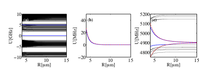
Figure 8: Our effective model (equations 1-3 in the main article) in the context of the full space of molecular potentials obtained from exact diagonalisation. (a) Set of molecular potentials in the energetic vicinity of the $|\,{80s_{1/2}}\,\rangle|\,{80s_{1/2}}\,\rangle$-pair state (whose energy is set to zero). The two blue lines are the potentials of interest, shown more detailed in panels (b-c). (b) Zoom onto (blue) $|\,{80s}\,\rangle|\,{80s}\,\rangle$ pair potential from exact diagonalisation, (red-dashed) model (3). (c) Zoom onto (blue) $|\,{80s_{1/2}}\,\rangle|\,{80p_{3/2}}\,\rangle\pm|\,{80p_{3/2}}\,\rangle|\,{80s_{1/2}}\,\rangle$ pair potentials from exact diagonalisation, (red-dashed) model (2,3).

Parameters for the model in equations (2,3) of the main article are fitted in the red-dashed lines, we obtain $C_{6,ss}=-7.6\times 10^{20}$ au. and $\mu=3374$ au. It is seen in panel (c) that for $R>5{\mu}m$ the relevant repulsive potential is energetically well separated from other energy surfaces, justifying our reduction of the state space. The nearest neighbouring pair states also visible in panel (c) belong to the $|\,{81d,f}\,\rangle|\,{79s}\,\rangle$, $|\,{81s}\,\rangle|\,{79d,f}\,\rangle$, $|\,{80d,f}\,\rangle|\,{80s}\,\rangle$ finestructure manifolds.

References

- Frenkel (1931) J. Frenkel, Phys. Rev. 37, 17 (1931).
- May and Kühn (2001) V. May and O. Kühn, Charge and Energy Transfer Dynamics in Molecular Systems (Wiley-VCH, Berlin, 2001).
- Park et al. (2011a) H. Park, P. J. Tanner, B. J. Claessens, E. S. Shuman, and T. F. Gallagher, Phys. Rev. A 84, 022704 (2011a).
- Park et al. (2011b) H. Park, E. S. Shuman, and T. F. Gallagher, Phys. Rev. A 84, 052708 (2011b).
- Li et al. (2005) W. Li, P. J. Tanner, and T. F. Gallagher, Phys. Rev. Lett. 94, 173001 (2005).
- Westermann et al. (2006) S. Westermann, T. Amthor, A. de Oliveira, J. Deiglmayr, M. Reetz-Lamour, and M. Weidemüller, Eur. Phys. J. D 40, 37 (2006).
- Mülken et al. (2007) O. Mülken, A. Blumen, T. Amthor, C. Giese, M. Reetz-Lamour, and M. Weidemüller, Phys. Rev. Lett. 99, 090601 (2007).
- Bettelli et al. (2013) S. Bettelli, D. Maxwell, T. Fernholz, C. S. Adams, I. Lesanovsky, and C. Ates, Phys. Rev. A 88, 043436 (2013).
- Günter et al. (2013) G. Günter, H. Schempp, M. Robert-de-Saint-Vincent, V. Gavryusev, S. Helmrich, C. S. Hofmann, S. Whitlock, and M. Weidemüller, Science 342, 954 (2013).
- Ravets et al. (2014) S. Ravets, H. Labuhn, D. Barredo, L. Béguin, T. Lahaye, and A. Browaeys (2014), arXiv:1405.7804.
- Barredo et al. (2014) D. Barredo, H. Labuhn, S. Ravets, T. Lahaye, A. Browaeys, and C. S. Adams (2014), arXiv:1408.1055.
- Gallagher (1994) T. F. Gallagher, Rydberg Atoms (Cambridge University Press, 1994).
- Beterov et al. (2009) I. I. Beterov, D. B. Tretyakov, I. I. Ryabtsev, V. M. Entin, A. Ekers, and N. N. Bezuglov, New J. Phys. 11, 013052 (2009).
- Ates et al. (2008) C. Ates, A. Eisfeld, and J. M. Rost, New J. Phys. 10, 045030 (2008).
- Wüster et al. (2010) S. Wüster, C. Ates, A. Eisfeld, and J. M. Rost, Phys. Rev. Lett. 105, 053004 (2010).
- Möbius et al. (2011) S. Möbius, S. Wüster, C. Ates, A. Eisfeld, and J. M. Rost, J. Phys. B: At. Mol. Opt. Phys. 44, 184011 (2011).
- Asadian et al. (2010) A. Asadian, M. Tiersch, G. G. Guerreschi, J. Cai, S. Popescu, and H. J. Briegel, New J. Phys. 12, 075019 (2010).
- Eisfeld (2011) A. Eisfeld, Chemical Physics 379, 33 (2011).
- Saikin et al. (2013) S. K. Saikin, A. Eisfeld, S. Valleau, and A. Aspuru-Guzik, Nanophotonics 2, 21 (2013).
- Kühn and Lochbrunner (2011) O. Kühn and S. Lochbrunner, Semiconductors and Semimetals 85, 47 (2011).
- Wüster et al. (2011) S. Wüster, A. Eisfeld, and J. M. Rost, Phys. Rev. Lett. 106, 153002 (2011).
- Domcke et al. (2004) W. Domcke, D. R. Yarkony, and H. Köppel, Conical Intersections (World Scientific, 2004).
- Li et al. (2013) L. Li, Y. O. Dudin, and A. Kuzmich, Nature 498, 466 (2013).
- Mukherjee et al. (2011) R. Mukherjee, J. Millen, R. Nath, M. P. A. Jones, and T. Pohl, J. Phys. B: At. Mol. Opt. Phys. 33, 184010 (2011).
- (25) See Supplemental Material for additional details regarding the employed quantum-classical algorithm, the Rydberg trimer subunit, our purity and entanglement measure, extraction of total atomic densities and the realization of isotropic dipole-dipole interactions, which includes Refs. Carrington (1974); Mead and Truhlar (1979); Hill and Wootters (1997); Wootters (1998); Goy et al. (1986).
- Carrington (1974) T. Carrington, Accounts of Chemical Research 7, 20 (1974).
- Mead and Truhlar (1979) C. A. Mead and D. G. Truhlar, The Journal of Chemical Physics 70, 2284 (1979).
- Hill and Wootters (1997) S. Hill and W. K. Wootters, Phys. Rev. Lett. 78, 5022 (1997).
- Wootters (1998) W. K. Wootters, Phys. Rev. Lett. 80, 2245 (1998).
- Goy et al. (1986) P. Goy, J. Liang, M. Gross, and S. Haroche, Phys. Rev. A 34, 2889 (1986).
- Tully and Preston (1971) J. C. Tully and R. K. Preston, J. Chem. Phys. 55, 562 (1971).
- Hammes-Schiffer and Tully (1994) S. Hammes-Schiffer and J. C. Tully, J. Chem. Phys. 101, 4657 (1994).
- Barbatti (2011) M. Barbatti, Wiley Interdisciplinary Reviews-Computational Molecular Science 1, 620 (2011).
- Jasper and Truhlar (2005) A. Jasper and D. Truhlar, J. Chem. Phys. 122 (2005), ISSN 0021-9606.
- Möbius et al. (2013) S. Möbius, M. Genkin, A. Eisfeld, S. Wuster, and J. M. Rost, Phys. Rev. A 87, 051602 (2013).
- Dennis et al. (2013) G. R. Dennis, J. J. Hope, and M. T. Johnsson, Comput. Phys. Commun. 184, 201 (2013).
- (37) Considering a trimer subunit only makes sense in a moment where three atoms have clearly closer mutual separations than all others.
- Teller (1937) E. Teller, J.Phys. Chem. 41, 109 (1937).
- McConnell et al. (2010) I. McConnell, G. Li, and G. W. Brudvig, Chemistry & Biology 17, 434 (2010).
- Schwarzkopf et al. (2011) A. Schwarzkopf, R. E. Sapiro, and G. Raithel, Phys. Rev. Lett. 107, 103001 (2011).
- Olmos et al. (2011) B. Olmos, W. Li, S. Hofferberth, and I. Lesanovsky, Phys. Rev. A 84, 041607(R) (2011).
- Günter et al. (2012) G. Günter, M. R. de Saint-Vincent, H. Schempp, C. S. Hofmann, S. Whitlock, and M. Weidemüller, Phys. Rev. Lett. 108, 013002 (2012).