Influence of a Minimal Length on the Creation of Scalar Particles

Abstract

In this paper we have studied the problem of scalar particles pair creation by an electric field in the presence of a minimal length. Two sets of exact solutions for the Klein Gordon equation are given in momentum space. Then the canonical method based on Bogoliubov transformation connecting the “in” with the “out” states is applied to calculate the probability to create a pair of particles and the mean number of created particles. The number of created particles per unit of time per unit of length, which is related directly to the experimental measurements, is calculated. It is shown that, with an electric field less than the critical value, the minimal length minimizes the particle creation. It is shown, also, that the limit of zero minimal length reproduces the known results corresponding to the ordinary quantum fields.

I Introduction

The fact that strong electric field creates particle-antiparticle pairs from the vacuum is predicted in the framework of quantum electrodynamics several decades ago EH ; Schwinger . This effect, which is known as the Schwinger effect, has a simple interpretation in the famous Dirac’s hole theory - e.g., in the presence of an electric field, virtual particles can tunnel out of the Dirac sea producing particle-hole pairs.

Since the publication of the seminal paper by Schwinger, a great interest is devoted to the problem of particle creation from vacuum by strong fields. Theoretically, the importance of this effect comes from its nonperturbative nature and its relation with other problems such as the black hole radiation and the dynamical Casimir effect. It is widely known, today, that the particle creation effects have many important applications from heavy nucleus to black hole physics Ruffini .

In experimental physics, the strong field pair production has attracted much attention, especially, in recent years. The field strength required to observe produced pairs is of order of the critical value $E_{c}=\frac{m^{2}}{e}=10^{16}\mathtt{Vcm}^{-1}$ (for electron pairs), which seems to be beyond the current technological capabilities. However, in recent years, explicit experimental realizations have been proposed to see the Schwinger effect for the first time exp1 ; exp2 ; exp3 . The basic principle of these experiments is the enhancement of the Schwinger mechanism by the combination of a strong slow pulsed laser with a weak fast pulsed laser. It is shown in exp1 that the faster pulse gives a multi-photon contribution, which reduces the barrier through which the particle tunnels and leads to an exponential enhancement. Then the Schwinger effect could be observed in the near future.

Quantitatively, in $\left(d+1\right)$ dimensional space-time, the number of created particles per unit of time per unit of volume is CF1

$$\mathcal{N}=\frac{\left(eE\right)^{\frac{d+1}{2}}}{\left(2\pi\right)^{d}}e^{-\pi\frac{m^{2}}{eE}}.$$ (1)

The important characteristic of this formula is the exponential $e^{-\pi\frac{m^{2}}{eE}}$, which explains the nonperturbative nature of the phenomenon and the existence of the critical value from which the effect becomes appreciable. Since this exponential is independent of the space-time dimension, the analysis of the effect seems to be the same in arbitrary dimensions. One expects, also, to obtain a similar exponential with a strong slow pulsed laser because, in such a case, the period of the field is very large compared to the typical time of the particle creation.

On the other hand, as is mentioned in Sabine , there are many indications that lead us to believe on the existence of a minimal length scale. This minimal length scale, which is expected to be smaller than the electroweak scale GUP1 ; GUP2 ; GUP3 ; GUP4 ; GUP5 , arises in many theories of quantum gravity such as string theory ST1 ; ST2 ; ST3 ; ST4 , loop quantum gravity LQG , black hole physics BH1 ; BH2 and in non-commutative field theories NC1 ; NC2 ; NC3 .

If such a minimal length exists in nature, it would be of great interest to see how it influences the physical measurements. This explains why various physical problems are reconsidered by taking into account the minimal length. As example, we cite the harmonic oscillator Kempf4 ; HO1 ; H1 , the Hydrogen atom H1 ; H2 ; H3 ; H4 ; H5 ; H6 ; H7 , the inverse square potential IS1 , the Dirac oscillator Rel1 , and the resonant scattering by a potential barrier RT ; Salah . Elsewhere, the influence of the minimal length on the Casimir effect has been communicated in several works Casimir1 ; Casimir2 . We note, also, that the quantum corrections to the black hole thermodynamics to all orders in the Planck length from a generalized uncertainty principle are calculated in nouicer . This kind of studies is motivated by the possibility it offers to put the existence of a minimal length into evidence and the regularization of certain problems in physics (see for instance IS1 ; Ferkous ). Furthermore, as is mentioned in Nicolini , since the presence of a minimal length is common to many theories, phenomena such as the Hawking effect and the particle creation, should be critically reviewed.

In this paper we propose to study the phenomenon of particle creation from vacuum by an electric field in the (1+1) dimensional Minkowski space-time with a nonzero minimal length. As in the case of the noncommutative space-time Chair , we expect that the introduction of a minimal length on the theory of fields could have important consequences on the particle creation. In addition, since the Schwinger effect is expected to be observed in the near future, the minimal length could find an experimental justification through this observation or at least find an important upper bound.

We consider in this paper the canonical method based on Bogoliubov transformation connecting the ”in” with the ”out” states. In the first stage, we give a short reminder about the particles creation problem and its derivation from the wave functions both in position representation or in momentum one. Then, we consider a scalar particle interacting with an electric field in the presence of a minimal length, where we give two sets of exact solutions for the corresponding Klein Gordon equation. In order to get the good definition of the ”in” and the ”out” states, we study the limit of zero minimal length. Next, we calculate the pair creation probability and the mean number of created particles from the Bogoliubov coefficients. Finally, we calculate the number of created particles per unit of time per unit of length as soon as the imaginary part of the Schwinger effective Lagrangian.

II Usual theory of particle creation

In order to derive the pair creation rate we have at our disposal several methods such as the method based on vacuum to vacuum transition amplitude and Schwinger-like effective action Schwinger ; Itzykson , the Hamiltonian diagonalization technique Grib ; Grib1 , the Feynman path integral method Haw ; Chit as well as the semiclassical WKB approximation Biswas1 ; Biswas2 and the ”in” and ”out” states formalism niki ; PCC that we shall use in this work.

The ”in” and ”out” states formalism has been much used in the theory of particle creation and vacuum instability in external fields. This formalism proved most fruitful in finding the probability to create a pair of particles and the mean number of created particles both in the presence of electromagnetic fields or in curved space-time where gravitational fields are present PCC . However, the ”in” and ”out” states method is based on analytic expressions of the wave functions which is not, in general, possible. Since the constant electric field is described by a linear potential, the corresponding Klein Gordon equation with minimal length admits exact and analytic solutions only in momentum representation. Therefore, the classification of these solutions as ”in” and ”out” states is not straightforward. Thus, before considering the creation of scalar particles in the presence of a minimal length, let us, first, recall briefly how to determine the ”in” and ”out” states in ordinary quantum field theory by the use of the momentum space. To our knowledge, there is no report, in literature, on the definition of these states in momentum space. It is obvious that the good definition of these states enables us to calculate the exact probability of particle creation as soon as the mean number of created particles with and without minimal length.

II.1 Position representation

In position representation the ”in” and ”out” states are well-defined. Here, we briefly recall their definition. Starting from the (1+1) dimensional Klein Gordon equation that describes the dynamics of a scalar matter field minimally coupled to an external electric field

$$\left[\left(\hat{p}_{\mu}-eA_{\mu}\left(x\right)\right)^{2}-m^{2}\right]\psi\left(t,x\right)=0,$$ (2)

where the 2-vector $A^{\mu}$ is given by

$$\ A^{\mu}\equiv\left(-Ex,0\right).$$ (3)

We choose to work in natural units system where $\hbar=c=1$. Let us remark that a constant electric field can be described by two straightforward gauges, namely, the space-dependent gauge $A_{\mu}=(-Ex,0)$ and the time-dependent gauge $A_{\mu}=(0,Et)$. In this work we consider the space-dependent gauge because it seems simpler in the presence of a minimal length.

As is known, in order to solve the equation (2), we write $\psi\left(t,x\right)=\exp(i\omega t)\varphi\left(x\right)$, where $\omega$ is the energy of the particle. Then $\varphi\left(x\right)$ will be a solution of

$$\left[\left(\omega+eEx\right)^{2}+\frac{\partial^{2}}{\partial x^{2}}-m^{2}\right]\varphi\left(x\right)=0.$$ (4)

By making the change

$$\xi=\sqrt{2ieE}\left(x+\frac{\omega}{eE}\right)$$ (5)

we obtain the well-known differential equation

$$\left[\frac{\partial^{2}}{\partial\xi^{2}}-\frac{1}{4}\xi^{2}+\gamma+\frac{1}{2}\right]\tilde{\varphi}\left(\xi\right)=0,$$ (6)

where $\tilde{\varphi}\left(\xi\right)\equiv\varphi\left(x\right)$ and

$$\gamma=-\frac{1}{2}+i\frac{1}{2}\frac{m^{2}}{eE}.$$ (7)

Equation (6) admits two sets of exact solutions that can be written in terms of Parabolic Cylinder Functions (PCFs) Grad . According to Hansen and Greiner the classification of these solutions as ”in” and ”out” states is as follows

$$\varphi_{in}^{-}\left(x\right) =D_{\gamma^{\ast}}\left[\left(1-i\right)\sqrt{eE}\left(x+\frac{\omega}{eE}\right)\right]$$ (8)

$$\varphi_{in}^{+}\left(x\right) =D_{\gamma}\left[-\left(1+i\right)\sqrt{eE}\left(x+\frac{\omega}{eE}\right)\right]$$ (9)

$$\varphi_{out}^{-}\left(x\right) =D_{\gamma}\left[\left(1+i\right)\sqrt{eE}\left(x+\frac{\omega}{eE}\right)\right]$$ (10)

$$\varphi_{out}^{+}\left(x\right) =D_{\gamma^{\ast}}\left[-\left(1-i\right)\sqrt{eE}\left(x+\frac{\omega}{eE}\right)\right],$$ (11)

Now, in order to determine the probability to create a pair of particles and the mean number of created particles, we use the so called Bogoliubov transformation connecting the ”in” with the ”out” states, which can be obtained by taking into account that $\gamma^{\ast}=-\gamma-1$ and using the formula Grad

$$D_{\gamma}\left(\xi\right)=\exp\left\{i\pi\gamma\right\}D_{\gamma}\left(-\xi\right)-\frac{\sqrt{2\pi}}{\Gamma\left(-\gamma\right)}\exp\left\{\frac{i\pi\gamma}{2}\right\}D_{-\gamma-1}\left(-i\xi\right).$$ (12)

The relation between $\varphi_{in}^{\pm}$ and $\varphi_{out}^{\pm}$ reads

$$\varphi_{in}^{+}\left(x\right) =c_{1}\varphi_{out}^{+}\left(x\right)+c_{2}\varphi_{out}^{-}\left(x\right)$$ (13)

$$\varphi_{in}^{-}\left(x\right) =c_{2}^{\ast}\varphi_{out}^{+}\left(x\right)+c_{1}^{\ast}\varphi_{out}^{-}\left(x\right),$$ (14)

where the Bogoliubov coefficients $c_{1}$ and $c_{2},$ given by

$$c_{1} =-\frac{\sqrt{2\pi}}{\Gamma\left(-\gamma\right)}\exp\left\{\frac{i\pi\gamma}{2}\right\}$$ (15)

$$c_{2} =\exp\left\{i\pi\gamma\right\},$$ (16)

fulfil the condition $\left|c_{1}\right|^{2}-\left|c_{2}\right|^{2}=1$.

In quantum field theory, the relation between the ”in” and the ”out” modes (13) and (14) can be converted into the following relation between the creation and annihilation operators

$$a_{\omega,out} =c_{1}\ a_{\omega,in}+c_{2}^{\ast}b_{\omega,in}^{+}$$ (17)

$$b_{\omega,out}^{+} =c_{2}\ a_{\omega,in}+c_{1}^{\ast}b_{\omega,in}^{+}.$$ (18)

Therefore, the probability of pair creation and the mean number of created particles will be given in terms of Bogoliubov coefficients. For instance, by considering the probability amplitude

$$\mathcal{A}=\left\langle 0_{out}\left|a_{\omega,out}b_{\omega,out}\right|0_{in}\right\rangle$$ (19)

and by taking into account that

$$b_{\omega,out}=\frac{1}{c_{1}^{\ast}}b_{\omega,in}+\frac{c_{2}^{\ast}}{c_{1}^{\ast}}a_{\omega,out}^{+}$$ (20)

we obtain

$$\mathcal{A}=\left\langle 0_{out}\left|a_{\omega,out}b_{\omega,out}\right|0_{in}\right\rangle=\frac{c_{2}^{\ast}}{c_{1}^{\ast}}\left\langle 0_{out}\mid 0_{in}\right\rangle.$$ (21)

As a result, the probability to create a pair of particles with the energy $\omega$ from vacuum is given by

$$\mathcal{P}_{\omega}=\left|\frac{c_{2}^{\ast}}{c_{1}^{\ast}}\right|^{2}.$$ (22)

Using the property

$$\left|\Gamma\left(\frac{1}{2}+iy\right)\right|^{2}=\frac{\pi}{\cosh\left(\pi y\right)}$$ (23)

we obtain the well-known result

$$\mathcal{P}_{\omega}=\frac{\exp\left(-\pi\frac{m^{2}}{eE}\right)}{1+\exp\left(-\pi\frac{m^{2}}{eE}\right)}.$$ (24)

This formulation enables us also to calculate the mean number of created particles and the vacuum persistence. The mean number of created particles in a state $\omega$ (the mean number of created particles per state) is defined by the matrix element $n\left(\omega\right)=\left\langle 0_{in}\left|a_{\omega,out}^{+}a_{\omega,out}\right|0_{in}\right\rangle$, which can be calculated to be

$$n\left(\omega\right)=\left|c_{2}\right|^{2}=\exp\left(-\pi\frac{m^{2}}{eE}\right).$$ (25)

It should be noted that Eq. (25) is derived by considering the commutators $\left[\hat{a}_{\omega,out},\hat{a}_{\omega^{\prime},out}^{+}\right]=\left[\hat{b}_{\omega,out},\hat{b}_{\omega^{\prime},out}^{+}\right]=\delta_{\omega\omega^{\prime}}$ with a finite time $T$ and discrete values of the energy $\omega$. If we consider the limit $T\rightarrow\infty$, the energy $\omega$ becomes continuous so that $n\left(\omega\right)$ can be interpreted as the number density of created particles or the number of created particles per state.

Eqs. (24) and (25) show that the present choice of ”in” and ”out” states leads to the exact results of the particle creation. Let us show, in the next paragraph, how these states can be expressed in momentum space.

II.2 Momentum representation

In momentum representation, the action of the operators $\hat{x}$ and $\hat{p}$ is given by

$$\hat{p} =p$$ (26)

$$\hat{x} =i\frac{\partial}{\partial p},$$ (27)

and, therefore, the Klein Gordon equation can be written as

$$\left[\left(\omega+ieE\frac{\partial}{\partial p}\right)^{2}-p^{2}-m^{2}\right]\tilde{\varphi}\left(p\right)=0$$ (28)

In order to solve this equation we factorize $\tilde{\varphi}\left(p\right)$ as follows

$$\tilde{\varphi}\left(p\right)=\exp\left(i\frac{\omega}{eE}p\right)F\left(p\right).$$ (29)

The new function $F\left(p\right)$ is then a solution of the following equation

$$\left[e^{2}E^{2}\frac{\partial^{2}}{\partial p^{2}}+p^{2}+m^{2}\right]F\left(p\right)=0.$$ (30)

By making the change

$$\eta=\sqrt{\frac{2}{ieE}}p$$ (31)

we obtain

$$\left[\frac{\partial^{2}}{\partial\eta^{2}}-\frac{1}{4}\eta^{2}+\gamma^{\ast}+\frac{1}{2}\right]f\left(\eta\right)=0,$$ (32)

with $f\left(\eta\right)\equiv F\left(p\right).$ We remark that the solutions of equation (32) can be written, also, in terms of PCFs.

Here, there is no reasonable criterion to find directly the good choice of ”in” and ”out” states starting from the wave equation in momentum space. The resort to the position space is then indispensable. Taking into account that the passage from position space to momentum space can be realized by the Fourier transformation, we obtain the following classification of the solutions

$$\tilde{\varphi}_{out}^{+}\left(p\right) =\exp\left(i\frac{\omega}{eE}p\right)D_{\gamma^{\ast}}\left[\left(1+i\right)\sqrt{\frac{1}{eE}}p\right]$$ (33)

$$\tilde{\varphi}_{out}^{-}\left(p\right) =\exp\left(i\frac{\omega}{eE}p\right)D_{\gamma}\left[\left(1-i\right)\sqrt{\frac{1}{eE}}p\right]$$ (34)

$$\tilde{\varphi}_{in}^{+}\left(p\right) =\exp\left(i\frac{\omega}{eE}p\right)D_{\gamma}\left[-\left(1-i\right)\sqrt{\frac{1}{eE}}p\right]$$ (35)

$$\tilde{\varphi}_{in}^{-}\left(p\right) =\exp\left(i\frac{\omega}{eE}p\right)D_{\gamma^{\ast}}\left[-\left(1+i\right)\sqrt{\frac{1}{eE}}p\right].$$ (36)

For the calculation of the Fourier transformation of the PCFs one can use equations (5.1) and (5.2) in Wolf .

Then, by the use of (12) we obtain the same Bogoliubov transformation as in (13) and (14)

$$\tilde{\varphi}_{in}^{+}\left(p\right) =c_{1}\tilde{\varphi}_{out}^{+}\left(p\right)+c_{2}\tilde{\varphi}_{out}^{-}\left(p\right)$$ (37)

$$\tilde{\varphi}_{in}^{-}\left(p\right) =c_{2}^{\ast}\tilde{\varphi}_{out}^{+}\left(p\right)+c_{1}^{\ast}\tilde{\varphi}_{out}^{-}\left(p\right).$$ (38)

Accordingly, this leads to the same probability and mean number as in (24) and (25). In reality, this result is unsurprising and it can be predicted directly from (13) and (14). It shows, however, that the Bogoliubov coefficients can be obtained directly from the ”in” and the ”out” states expressed in momentum space. This will be very interesting in the presence of the minimal length where there is no exact and analytic solution in position space.

III Particles creation with minimal length

Before considering the effect of the minimal length on creation of scalar particles by an electric field, let us, first, give a short reminder about this novel concept. There are many considerations that suggest the existence of a minimal length. For example, in black hole physics Adler , it is shown that the Heisenberg uncertainty principle modifies to be

$$\Delta X\geq\frac{1}{2}\left(\frac{1}{\Delta P}+\beta\Delta P\right),$$ (39)

where $\beta$ is very small positive parameter and $\hbar=1$. Such a generalized uncertainty principle (GUP) leads to a nonzero minimal length given by

$$\left(\Delta X\right)_{\min}=\sqrt{\beta}.$$ (40)

In addition, since the relation (39) is invariant under the change $\sqrt{\beta}\Delta P\rightarrow\frac{1}{\sqrt{\beta}\Delta P}$, there would be a mixing between the ultraviolet and infrared behaviors of the field theories, which is called the UV/IR mixing.

The derivation of this GUP by quantum mechanical tools in the one dimensional space and its generalization to arbitrary dimensional case can be found in a series of papers by Kempf and co-workers Kempf4 ; Kempf1 ; Kempf2 ; Kempf3 . It is shown in these papers how the quantum mechanics with GUP can be formulated. Here, we recall, briefly, that the GUP in (39) can be reproduced by considering new operators $\hat{X}$ and $\hat{P}$ defined by

$$\hat{X} =\hat{x}$$ (41)

$$\hat{P} =f\left(\hat{p}\right),$$ (42)

where $\hat{x}$ and $\hat{p}$ are the usual operators of quantum mechanics fulfilling the commutation relation $\left[\hat{x},\hat{p}\right]=i$ and $f\left(\hat{p}\right)$ is an injective function. The simpler case is to consider the expansion

$$f\left(\hat{p}\right)=\hat{p}\left(1+\frac{\beta}{3}\hat{p}^{2}+...\right).$$ (43)

Taking into account that $\left[\hat{X},\hat{P}\right]=if^{\prime}\left(\hat{p}\right)$ and $\tilde{p}\approx\hat{P}\left(1-\frac{\beta}{3}\hat{P}^{2}+...\right)$, we find that

$$\left[\hat{X},\hat{P}\right]=i\left(1+\beta\hat{P}^{2}\right).$$ (44)

Then it is easy to show that this modified canonical commutation relation leads to equation (39). It should be noted that the produced GUP depends on the choice of the function $f$. The present choice is suitable for a minimal length. In literature we find other choices that correspond to a minimal length and/or maximal momentum (see for example pouria ; pouria2 ).

From equations (41), (42), (43) and (44), we can derive several representations for the operators $\hat{X}$ and $\hat{P}$. Among these representations we quote the position representation defined by

$$\hat{X} =x,$$ (45)

$$\hat{P} =\left(1+\frac{1}{3}\beta\hat{p}^{2}\right)\hat{p},$$ (46)

with

$$\ \hat{p}=-i\frac{\partial}{\partial x},$$ (47)

and the momentum representation, where the action of the operators $\hat{X}$ and $\hat{P}$ is as follows

$$\hat{P} =p,$$ (48)

$$\hat{X} =i\left[\left(1+\beta p^{2}\right)\frac{\partial}{\partial p}\right].$$ (49)

Besides the fact that the present commutation relation provides us with exact solvable model (see for example the works cited above), it offers the possibility to show how the minimal length influences the physical measurements. Then, to see the effect of this minimal length on the particle creation, it is sufficient to consider equation (44). The use of a more general commutation relation risks leading to a nonsolvable problem and much mathematical difficulties.

In the next paragraph we solve the Klein Gordon equation in the presence of an electric field by taking into account the canonical commutation relation (44).

III.1 Klein Gordon equation with a minimal length

Before solving the Klein Gordon equation with a minimal length and studying the creation of scalar particles, let us show that the minimal length theory is consistent with the concept of gauge invariance. To this aim, we consider the free Klein Gordon equation

$$\left(-\frac{\partial^{2}}{\partial t^{2}}-\hat{P}^{2}-m^{2}\right)\psi\left(t,x\right)=0,$$ (50)

in the position space representation and we assume that a charged particle described the Klein Gordon equation (50) couples minimally to the electromagnetic field following the general procedure

$$i\frac{\partial}{\partial t} \rightarrow i\frac{\partial}{\partial t}-eA_{0}$$ (51)

$$\text{\ }i\frac{\partial}{\partial x} \rightarrow i\frac{\partial}{\partial x}-eA_{1}.$$ (52)

Then, to the first order on $\beta$, the Klein Gordon equation becomes

$$\left[\left(i\frac{\partial}{\partial t}-eA_{0}\right)^{2}-\left(i\frac{\partial}{\partial x}-eA_{1}\right)^{2}-\frac{2\beta}{3}\left(i\frac{\partial}{\partial x}-eA_{1}\right)^{4}-m^{2}\right]\psi\left(t,x\right)=0.$$ (53)

Here, we remark that this equation is invariant under the gauge transformation

$$\psi^{\prime}\left(t,x\right) =e^{ie\alpha}\psi\left(t,x\right)$$

$$A_{\mu}^{\prime}\left(t,x\right) =A_{\mu}\left(t,x\right)+\partial_{\mu}\alpha.$$ (54)

Let us, now, consider a scalar particle of mass $m$ and charge $e$ subjected to a constant electric field $E$. In the presence of a minimal length the use of the time-dependent gauge, with the assumption that $\psi\left(t,x\right)=e^{-ipx}\chi\left(t\right)$, leads to the following differential equation

$$\left[\frac{\partial^{2}}{\partial t^{2}}+\left(p+eEt\right)^{2}+\frac{2\beta}{3}\left(p+eEt\right)^{4}+m^{2}\right]\chi\left(t\right)=0.$$ (55)

To our knowledge there is no exact solution for this differential equation. For this reason we consider the space-dependent gauge. With this choice equation (53) reduces to

$$\left[\frac{\partial^{2}}{\partial x^{2}}-\frac{2\beta}{3}\frac{\partial^{4}}{\partial x^{4}}+\left(\omega+eEx\right)^{2}-m^{2}\right]\varphi\left(x\right)=0.$$ (56)

The latter equation is of fourth order and, consequently, does not admit exact and analytic solutions. Therefore, we use the momentum representation, where the one dimensional stationary Klein Gordon equation reads

$$\left[\left(\omega+eE\hat{X}\right)^{2}-\hat{P}^{2}-m^{2}\right]\varphi=0,$$ (57)

and the action of the operators $\hat{X}$ and $\hat{P}$ is shown in (48) and (49).

Then, in the $p$-representation, equation (57) can be written as

$$\left[e^{2}E^{2}\left(1+\beta p^{2}\right)^{2}\frac{\partial^{2}}{\partial p^{2}}+2eE\left(\beta eEp-i\omega\right)\left(1+\beta p^{2}\right)\frac{\partial}{\partial p}+p^{2}+m^{2}-\omega^{2}\right]\tilde{\varphi}\left(p\right)=0.$$ (58)

By making the change $p\rightarrow y,$ with

$$y=\frac{1-i\sqrt{\beta}p}{2}$$ (59)

we obtain a Riemann type differential equation

$$\left[\frac{\partial^{2}}{\partial y^{2}}+\left(\frac{1-a_{1}-a_{1}^{\prime}}{y}-\frac{1-a_{3}-a_{3}^{\prime}}{1-y}\right)\frac{\partial}{\partial y}+\right.$$

$$\left.\left.\left(\frac{a_{1}a_{1}^{\prime}}{y}-a_{2}a_{2}^{\prime}+\frac{a_{3}a_{3}^{\prime}}{\left(1-y\right)}\right)\frac{1}{y\left(1-y\right)}\right]g\left(y\right)=0\right.$$ (60)

where the coefficients $a_{i}$ and $a_{i}^{\prime}$ are given by

$$a_{1} =-\frac{\omega}{2eE\sqrt{\beta}}+i\frac{\sqrt{1-\beta m^{2}}}{2eE\beta}$$ (61)

$$a_{1}^{\prime} =-\frac{\omega}{2eE\sqrt{\beta}}-i\frac{\sqrt{1-\beta m^{2}}}{2eE\beta}$$ (62)

$$a_{3} =\frac{\omega}{2eE\sqrt{\beta}}+i\frac{\sqrt{1-\beta m^{2}}}{2eE\beta}$$ (63)

$$a_{3}^{\prime} =\frac{\omega}{2eE\sqrt{\beta}}-i\frac{\sqrt{1-\beta m^{2}}}{2eE\beta},$$ (64)

and

$$a_{2}=1-a_{2}^{\prime}=\frac{1}{2}+\nu,$$ (65)

with

$$\nu=\frac{i}{eE\beta}\sqrt{1-\left(\frac{eE\beta}{2}\right)^{2}}.$$ (66)

These coefficients satisfy the condition $a_{1}+a_{1}^{\prime}+a_{2}+a_{2}^{\prime}+a_{3}+a_{3}^{\prime}=1$.

Following Grad equation (60) admits two independent solutions which can be written in terms of hypergeometric functions as follows

$$\tilde{\varphi}_{{}_{1}} =\left(\frac{1-i\sqrt{\beta}p}{2}\right)^{-\frac{\omega}{2eE\sqrt{\beta}}+i\frac{\sqrt{1-\beta m^{2}}}{2eE\beta}}\left(\frac{1+i\sqrt{\beta}p}{2}\right)^{\frac{\omega}{2eE\sqrt{\beta}}+i\frac{\sqrt{1-\beta m^{2}}}{2eE\beta}}$$

$$F\left(\frac{1}{2}+\nu+i\frac{\sqrt{1-\beta m^{2}}}{eE\beta},\frac{1}{2}-\nu+i\frac{\sqrt{1-\beta m^{2}}}{eE\beta};1+i\frac{\sqrt{1-\beta m^{2}}}{eE\beta};\frac{1-i\sqrt{\beta}p}{2}\right)$$ (67)

and

$$\tilde{\varphi}_{{}_{2}} =\left(\frac{1-i\sqrt{\beta}p}{2}\right)^{-\frac{\omega}{2eE\sqrt{\beta}}-i\frac{\sqrt{1-\beta m^{2}}}{2eE\beta}}\left(\frac{1+i\sqrt{\beta}p}{2}\right)^{\frac{\omega}{2eE\sqrt{\beta}}+i\frac{\sqrt{1-\beta m^{2}}}{2eE\beta}}$$

$$F\left(\frac{1}{2}+\nu,\frac{1}{2}-\nu;1-i\frac{\sqrt{1-\beta m^{2}}}{eE\beta};\frac{1-i\sqrt{\beta}p}{2}\right).$$ (68)

This choice of solutions, however, is not unique. If we use the fact that equation (60) is invariant under the change $y\rightarrow 1-y$ and $\left(a,a^{\prime}\right)\leftrightarrow\left(c,c^{\prime}\right)$, we can find an other set of solutions $\left\{\tilde{\varphi}_{{}_{3}},\tilde{\varphi}_{4}\right\}$, where

$$\tilde{\varphi}_{{}_{3}} =\left(\frac{1+i\sqrt{\beta}p}{2}\right)^{\frac{\omega}{2eE\sqrt{\beta}}+i\frac{\sqrt{1-\beta m^{2}}}{2eE\beta}}\left(\frac{1-i\sqrt{\beta}p}{2}\right)^{-\frac{\omega}{2eE\sqrt{\beta}}+i\frac{\sqrt{1-\beta m^{2}}}{2eE\beta}}$$

$$F\left(\frac{1}{2}+\nu+i\frac{\sqrt{1-\beta m^{2}}}{eE\beta},\frac{1}{2}-\nu+i\frac{\sqrt{1-\beta m^{2}}}{eE\beta};1+i\frac{\sqrt{1-\beta m^{2}}}{eE\beta};\frac{1+i\sqrt{\beta}p}{2}\right)$$ (69)

and

$$\tilde{\varphi}_{{}_{4}} =\left(\frac{1+i\sqrt{\beta}p}{2}\right)^{\frac{\omega}{2eE\sqrt{\beta}}-i\frac{\sqrt{1-\beta m^{2}}}{2eE\beta}}\left(\frac{1-i\sqrt{\beta}p}{2}\right)^{-\frac{\omega}{2eE\sqrt{\beta}}+i\frac{\sqrt{1-\beta m^{2}}}{2eE\beta}}$$

$$F\left(\frac{1}{2}+\nu,\frac{1}{2}-\nu;1-i\frac{\sqrt{1-\beta m^{2}}}{eE\beta};\frac{1+i\sqrt{\beta}p}{2}\right).$$ (70)

Thus, we have succeeded to find two sets of exact solutions for the Klein Gordon equation with a minimal length in the presence of a constant electric field. In the next paragraph we shall use these solutions to study the pair creation.

III.2 The choice of ”in” and ”out” states and particle creation

In order to classify our solutions as ”in” and ”out” states, we consider the limit $\beta\rightarrow 0$ and we compare the obtained solutions with the results of section II (The calculation of this limit is shown in the appendix). As a result, we find that the ”in” states are given by $\tilde{\varphi}_{1}\left(p\right)$ and $\tilde{\varphi}_{4}\left(p\right)$

$$\begin{array}[c]{c}\tilde{\varphi}_{in}^{+}=\tilde{\varphi}_{1}\left(p\right)\\ \tilde{\varphi}_{in}^{-}=\tilde{\varphi}_{4}\left(p\right)\end{array}$$ (71)

and the ”out” states are given by $\tilde{\varphi}_{2}\left(p\right)$ and $\tilde{\varphi}_{3}\left(p\right)$

$$\begin{array}[c]{c}\tilde{\varphi}_{out}^{+}=\tilde{\varphi}_{2}\left(p\right)\\ \tilde{\varphi}_{out}^{-}=\tilde{\varphi}_{3}\left(p\right).\end{array}$$ (72)

Now, in order to obtain the relation between ”in” and ”out” modes and the corresponding Bogoliubov coefficients, let us use the relation between hypergeometric functions Grad

$$F\left(u,v;w;\xi\right) =\frac{\Gamma\left(w\right)\Gamma\left(w-v-u\right)}{\Gamma\left(w-u\right)\Gamma\left(w-v\right)}F\left(u,v;u+v-w+1;1-\xi\right)~{}~{}$$

$$+\left(1-\xi\right)^{w-u-v}\frac{\Gamma\left(w\right)\Gamma\left(u+v-w\right)}{\Gamma\left(u\right)\Gamma\left(v\right)}$$

$$F\left(w-u,w-v;w-v-u+1;1-\xi\right)$$ (73)

to get

$$\varphi_{in}^{+}=c_{1}\varphi_{out}^{+}+c_{2}\varphi_{out}^{-}$$ (74)

where, in this case the Bogoliubov coefficients are given by

$$c_{1} =e^{i\vartheta}\frac{\Gamma\left(\frac{1}{2}+\nu\right)\Gamma\left(\frac{1}{2}-\nu\right)}{\Gamma\left(\frac{1}{2}+\nu+i\frac{\sqrt{1-\beta m^{2}}}{eE\beta}\right)\Gamma\left(\frac{1}{2}-\nu+i\frac{\sqrt{1-\beta m^{2}}}{eE\beta}\right)}$$ (75)

$$c_{2} =\frac{\Gamma\left(\frac{1}{2}+\nu\right)\Gamma\left(\frac{1}{2}-\nu\right)}{\Gamma\left(1+i\frac{\sqrt{1-\beta m^{2}}}{eE\beta}\right)\Gamma\left(-i\frac{\sqrt{1-\beta m^{2}}}{eE\beta}\right)}$$ (76)

where

$$e^{i\vartheta}=-\frac{\Gamma\left(i\frac{\sqrt{1-\beta m^{2}}}{eE\beta}\right)}{\Gamma\left(-i\frac{\sqrt{1-\beta m^{2}}}{eE\beta}\right)}.$$ (77)

By the use of (23) and the following properties of Gamma functions

$$\Gamma\left(x+1\right)=x\Gamma\left(x\right)$$ (78)

and

$$\left|\Gamma\left(iy\right)\right|^{2}=\frac{\pi}{y\sinh\left(\pi y\right)}$$ (79)

we find

$$\mathcal{P}_{\omega}=\frac{2\sinh^{2}\left(\frac{\pi}{eE\beta}\sqrt{1-\beta m^{2}}\right)}{\cosh\left(\frac{2\pi}{eE\beta}\sqrt{1-\beta m^{2}}\right)+\cosh\left(\frac{2\pi}{eE\beta}\sqrt{1-\left(\frac{eE\beta}{2}\right)^{2}}\right)}.$$ (80)

For the mean number of created particles, we have

$$n\left(\omega\right)=\frac{\sinh^{2}\left(\frac{\pi}{eE\beta}\sqrt{1-\beta m^{2}}\right)}{\cosh^{2}\left(\frac{\pi}{eE\beta}\sqrt{1-\left(\frac{eE\beta}{2}\right)^{2}}\right)}.$$ (81)

Since the minimal length is supposed to be small we restrict our discussion to the case when $\beta m^{2}\leq 1$. It follows from equation (81) that when $\beta m^{2}=1$, the mean number $n\left(\omega\right)=0$. This is, physically, plausible because particle-antiparticle pairs are defined only when the measurable Compton wavelength of the particle is larger than the minimal length.

In figure (1), we plot the ratio $n\left(\omega\right)/n_{0}\left(\omega\right)$, where $n_{0}\left(\omega\right)$ is the usual density of created particles (i.e. without minimal length) as a function of the variable $\beta m^{2}$ for various values of $\frac{E_{c}}{E}\equiv r$. As a result, we remark that the minimal length amplifies the scalar particle creation when $\frac{E_{c}}{E}<1$ and minimizes it when $\frac{E_{c}}{E}>1$. With the available technological capabilities the maximal strength of the produced electric field is less than $E_{c}$ and consequently, the effect of the minimal length is to reduce the scalar particle creation.

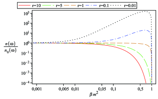
Figure 1: Plotting $n\left(\omega\right)/n_{0}\left(\omega\right)$ as a function of the variable $\beta m^{2}$. The parameter $r~{}$is defined by $r=\frac{E_{c}}{E}$.

As is shown in figure (1), for small values $\beta m^{2}$, we see that the minimal length can decrease or increase the pair creation rate. This depends on the value of $\frac{E_{c}}{E}$. To put this effect into evidence, let us take into account that $\beta$ is a small parameter and use the approximations

$$\frac{2\pi}{eE\beta}\sqrt{1-\left(\frac{eE\beta}{2}\right)^{2}}\approx\frac{2\pi}{eE\beta}-\pi\frac{eE\beta}{4}$$ (82)

and

$$\frac{2\pi}{eE\beta}\sqrt{1-\beta m^{2}}\approx\allowbreak\frac{2\pi}{eE\beta}-\pi\frac{m^{2}}{eE}-\frac{2\pi}{eE}\frac{1}{8}m^{4}\beta.$$ (83)

In such a case, the mean number of created particles by an electric field takes the form

$$n\left(\omega\right)=\exp\left[-\pi\frac{m^{2}}{eE}\left(1+\frac{1}{4}\beta m^{2}\left(1-\frac{e^{2}E^{2}}{m^{4}}\right)\right)\right]$$ (84)

and the probability to create a pair of particles becomes

$$\mathcal{P}_{\omega}=\frac{\exp\left[-\pi\frac{m^{2}}{eE}\left(1+\frac{1}{4}\beta m^{2}\left(1-\frac{e^{2}E^{2}}{m^{4}}\right)\right)\right]}{1+\exp\left[-\pi\frac{m^{2}}{eE}\left(1+\frac{1}{4}\beta m^{2}\left(1-\frac{e^{2}E^{2}}{m^{4}}\right)\right)\right]},$$ (85)

This means that a nonzero minimal length amplifies the scalar particle creation when $\frac{E_{c}}{E}<1$ and minimizes it when $\frac{E_{c}}{E}>1$, as is shown in figure (1). In addition, we note that equations (84) and (85) reduce, respectively, to (24) and (25), when $\beta\rightarrow 0$.

Here, we have several remarks to add. As first remark, we note that we have used, for the ”in” and the ”out” states in ordinary quantum field theory, the choice of Hansen ; Greiner . The use of the choice of Niki1 ; hao leads to the same results.

Secondly, it should be noted that, since the Klein Gordon equation is gauge invariant, one expects to obtain the same results by the use of the time-dependent gauge. The proof of this can be done by considering the WKB method starting from Eq. (55). For instance, the pair creation probability is given, in the WKB approximation, by

$$P\approx\exp\left[-2\operatorname{Im}\oint\sqrt{m^{2}+\left(p-eEt\right)^{2}+\frac{2\beta}{3}\left(p-eEt\right)^{4}}dt\right].$$ (86)

Then by the use of the following integral

$$\int_{0}^{b}\sqrt{\left(x^{2}-b^{2}\right)\left(x^{2}-a^{2}\right)}dx=\frac{a}{3}\left[\left(a^{2}+b^{2}\right)E\left(\frac{b}{a}\right)-\left(a^{2}-b^{2}\right)K\left(\frac{b}{a}\right)\right],$$ (87)

where $K\left(k\right)$ and $E\left(k\right)$ are, respectively, the Euler integrals of first and second kind, and by taking into account that $E\left(k\right)$ and $K\left(k\right)$ have the following expansions for small values of $k$,

$$K\left(k\right) =\frac{\pi}{2}\left(1+\frac{1}{4}k^{2}+\frac{9}{64}k^{4}+...\right)$$ (88)

$$E\left(k\right) =\frac{\pi}{2}\left(1-\frac{1}{4}k^{2}-\frac{3}{64}k^{4}+...\right)$$ (89)

we obtain

$$P\approx\exp\left[-\pi\frac{m^{2}}{eE}\left(1+\frac{1}{4}\beta m^{2}\right)\right].$$ (90)

This shows that the time dependent gauge gives approximately the same result as the space dependent gauge.

Finally, let us remark that the quantity which is directly related to the experimental measurements is the number of created particles per unit of time per unit of length (in 1+1 dimensions). In the next subsection, we show how this quantity can be calculated.

III.3 The total number of created particles and the Schwinger effective action

Let us, first, calculate the total number of created particles by doing summation over all states. The total number of created particles is given by

$$N=\int\frac{T}{2\pi}d\omega~{}n\left(\omega\right)=\int\frac{dtd\omega}{2\pi}n\left(\omega\right).$$ (91)

Here, it should be noted that $\frac{dtd\omega}{2\pi}$ can be interpreted as the number of states in the area sandwiched between the equal-energy contours $\omega$ and $\omega+d\omega$, and the equal-time contours $t$ and $t+dt$ in the $\left(t,\omega\right)$ plane. Therefore, the minimal length as introduced in (44) has no influence on the mesure $\frac{dtd\omega}{2\pi}$ because the time and energy operators in the Klein Gordon equation satisfy the ordinary canonical commutation relation.

According to Ni , the integration over energy $\omega$ can be replaced by

$$\int d\omega=eE\int dx,$$ (92)

where the variable $x$ denotes the position at which pairs with energy $\omega$ are created. The total number of created particles is then given by

$$N=\int dtdx\frac{eE}{2\pi}\frac{\sinh^{2}\left(\pi\frac{\sqrt{1-\beta m^{2}}}{eE\beta}\right)}{\cosh^{2}\left(\frac{\pi}{eE\beta}\sqrt{1-\left(\frac{eE\beta}{2}\right)^{2}}\right)}.$$ (93)

On the other hand, if we write $N$ as

$$N=\int dN=\int\frac{dN}{dtdx}dtdx,$$ (94)

we interpret $\frac{dN}{dtdx}\equiv\mathcal{N}$ as the number of created particles per unit of time per unit of length. It follows from equations (93) and (94) that

$$\mathcal{N}=\frac{dN}{dtdx}=\frac{eE}{2\pi}\frac{\sinh^{2}\left(\pi\frac{\sqrt{1-\beta m^{2}}}{eE\beta}\right)}{\cosh^{2}\left(\frac{\pi}{eE\beta}\sqrt{1-\left(\frac{eE\beta}{2}\right)^{2}}\right)}.$$ (95)

Here, we remark that for small values of $\beta$, $\mathcal{N}$ can be put in the form

$$\mathcal{N}=\frac{eE}{2\pi}\exp\left[-\pi\frac{m^{2}}{eE}\left(1+\frac{1}{4}\beta m^{2}\left(1-\frac{e^{2}E^{2}}{m^{4}}\right)\right)\right].$$ (96)

This equation can be written as

$$\mathcal{N}=\mathcal{N}_{0}\left[1-\frac{\pi}{4}\beta\frac{m^{4}}{eE}\left(1-\frac{e^{2}E^{2}}{m^{4}}\right)\right]$$ (97)

where $\mathcal{N}_{0}$ is the usual number of created particles per unit of time per unit of length

$$\mathcal{N}_{0}=\frac{eE}{2\pi}\exp\left(-\pi\frac{m^{2}}{eE}\right)$$ (98)

and the factor $\left(1-\frac{\pi}{4}\beta\frac{m^{4}}{eE}\left(1-\frac{e^{2}E^{2}}{m^{4}}\right)\right)$ is the correction induced by the minimal length.

If in future experiments the pair creation is observed, the relation (97) could be used to quantify the predicted minimal length. Since the quantity $\frac{m^{4}}{eE}$ is of order of $10^{-2}$ [GeV]² for $E=10^{-2}E_{c}$ and $m\approx m_{e}$, just the observation of the effect would imply that the minimal length is smaller than $10^{-15}$m. Accurate measurements would lead to an important upper bound.

Let us, now, show how the minimal length modifies the imaginary part of the Schwinger effective action. It is well-known in quantum field theory that the vacuum to vacuum transition amplitude can be expressed through an intermediate effective action,

$$\left\langle 0_{out}\left|0_{in}\right\rangle\right.=\exp\left(iS_{eff}\right)=\exp\left(i\int d^{2}x~{}\mathcal{L}_{eff}\right),$$ (99)

where $\mathcal{L}_{eff}$ is the Euler-Heisenberg effective Lagrangian EH . The probability of pair creation per unit of time and length can be then extracted from the imaginary part of this Lagrangian

$$\mathcal{P}_{Creat.}=\frac{1}{LT}\left[1-\left|\left\langle 0_{out}\left|0_{in}\right\rangle\right.\right|^{2}\right]\simeq 2\operatorname{Im}\mathcal{L}_{eff}.$$ (100)

In the present case, it is easy to show that the vacuum persistence $\mathcal{C}_{k}$ can be written in the form

$$\mathcal{C}_{\omega}=1-\mathcal{P}_{\omega}=\frac{1}{1+\sigma},$$

where

$$\sigma=\frac{\sinh^{2}\left(\pi\frac{\sqrt{1-\beta m^{2}}}{eE\beta}\right)}{\cosh^{2}\left(\frac{\pi}{eE\beta}\sqrt{1-\left(\frac{eE\beta}{2}\right)^{2}}\right)}.$$ (101)

The vacuum to vacuum transition probability is then

$$\exp\left(-2\operatorname{Im}S_{eff}\right) =\prod_{\omega}\mathcal{C}_{\omega}$$ (102)

$$=\prod_{\omega}\exp\left[-\ln\left(1+\sigma\right)\right]$$ (103)

$$=\exp\left[-\sum_{\omega}\ln\left(1+\sigma\right)\right]$$ (104)

and, accordingly,

$$2\operatorname{Im}S_{eff}=\int dxdt~{}2\operatorname{Im}\mathcal{L}_{eff}=\sum_{\omega}\ln\left(1+\sigma\right).$$ (105)

Here the symbol $\sum\limits_{\omega}$ denotes $\int\frac{dtd\omega}{2\pi}$. Then the imaginary part of the effective Lagrangian can be written as

$$2\operatorname{Im}\mathcal{L}_{eff}=\frac{eE}{2\pi}\ln\left(1+\frac{\sinh^{2}\left(\pi\frac{\sqrt{1-\beta m^{2}}}{eE\beta}\right)}{\cosh^{2}\left(\frac{\pi}{eE\beta}\sqrt{1-\left(\frac{eE\beta}{2}\right)^{2}}\right)}\right).$$ (106)

In the small $\beta$ limit, we get

$$2\operatorname{Im}\mathcal{L}_{eff}=\frac{eE}{2\pi}\ln\left\{1+\exp\left[-\pi\frac{m^{2}}{eE}\left(1+\frac{1}{4}\beta m^{2}\left(1-\frac{e^{2}E^{2}}{m^{4}}\right)\right)\right]\right\}.$$ (107)

In addition, if we expand the logarithm function, we find the expression

$$2\operatorname{Im}\mathcal{L}_{eff}=\frac{eE}{2\pi}\sum_{n=1}\frac{\left(-1\right)^{n+1}}{n}\exp\left[-n\pi\frac{m^{2}}{eE}\left(1+\frac{1}{4}\beta m^{2}\left(1-\frac{e^{2}E^{2}}{m^{4}}\right)\right)\right],$$ (108)

which resembles to the well-know result corresponding to the scalar particle creation in the (1+1) dimensional space-time CF1 , with the change $m^{2}\rightarrow m^{2}\left(1+\frac{1}{4}\beta m^{2}\left(1-\frac{e^{2}E^{2}}{m^{4}}\right)\right)$.

As is mentioned above, in the ordinary case, the exponential $\exp\left(-\pi m^{2}/eE\right)$ appears in any $\left(d+1\right)$ dimensional space-time. In the presence of the minimal length, we expect to have an exponential similar to $\exp\left[-\pi\frac{m^{2}}{eE}\left(1+\frac{1}{4}\beta m^{2}\left(1-\frac{e^{2}E^{2}}{m^{4}}\right)\right)\right]$ in arbitrary dimensions.

IV Conclusion

In this paper, we have studied the problem of scalar particles pair creation by an electric field in the presence of a minimal length by the use of the canonical method based on Bogoliubov transformation. Although the corresponding Klein Gordon equation is exactly solved in momentum space, it was difficult to derive directly the pair creation probability. For this reason, we have considered in the first stage the particle creation in ordinary quantum field theory where we have written the ”in” and the ”out” states in momentum representation. In the presence of a minimal length, we have distinguished the ”in” from the ”out” states by studying the limit $\beta\rightarrow 0$. Then, we were able to extract the Bogoliubov coefficients and to calculate the pair production probability and the mean number of created particles. The number of created particles per unit of time per unit of length, which is related directly to the experimental measurements, is calculated.

It is shown that the minimal length minimizes the particle creation when $\frac{E_{c}}{E}\geq 1$. This effect can be explained by the fact that, in the presence of the minimal length, the threshold energy of the pair creation modifies to be $2m\left(1+\frac{1}{4}\beta m^{2}\left(1-\frac{e^{2}E^{2}}{m^{4}}\right)\right)$ instead of $2m$. This could play a role in the explanation why we do not see the assisted particle creation with the already available technologies.

It is shown, also, that Schwinger mechanism can not create particles with mass $m\sim\frac{1}{\sqrt{\beta}}$. Theoretically, this result could have a strong impact on cosmology. If we reconcile that cosmological particle creation is similar to the Schwinger effect, the creation of superheavy particles with the mass of the Grand Unification scale in the early Universe, which is supposed to have some important cosmological consequences SHP , is then suppressed by the GUP effects.

Appendix A The $\beta\rightarrow 0$ limit

To find the good choice of ”in” and ”out” states let us study the limit $\beta\rightarrow 0$ that reproduces the ordinary case.

By using of the formula Grad

$$F\left(2a,2b;a+b+\frac{1}{2};\frac{1-z}{2}\right) =A~{}F\left(a,b;\frac{1}{2};z^{2}\right)$$

$$+B~{}z~{}F\left(a+\frac{1}{2},b+\frac{1}{2};\frac{3}{2};z^{2}\right)$$ (109)

where

$$A =\frac{\Gamma\left(a+b+\frac{1}{2}\right)\Gamma\left(\frac{1}{2}\right)}{\Gamma\left(a+\frac{1}{2}\right)\Gamma\left(b+\frac{1}{2}\right)}$$ (110)

$$B =\frac{\Gamma\left(a+b+\frac{1}{2}\right)\Gamma\left(-\frac{1}{2}\right)}{\Gamma\left(a\right)\Gamma\left(b\right)}$$ (111)

and taking into account that

$$\left.\lim_{\beta\rightarrow 0}\left(i\frac{\sqrt{1-\beta m^{2}}}{2eE\beta}-\frac{i}{2eE\beta}\sqrt{1-\left(\frac{eE\beta}{2}\right)^{2}}\right)=-i\frac{1}{4}\frac{m^{2}}{eE},\right.$$ (112)

$$\left.\lim_{\beta\rightarrow 0}\frac{\Gamma\left(\frac{3}{4}+i\frac{m^{2}}{4eE}+\frac{i}{eE\beta}\right)}{\Gamma\left(\frac{1}{4}+i\frac{m^{2}}{4eE}+\frac{i}{eE\beta}\right)}\sqrt{\beta}=\frac{1}{\sqrt{2eE}}\left(1+i\right).\right.$$ (113)

and Grad

$$\lim_{v\rightarrow\infty}~{}~{}_{2}F_{1}\left(u,v;w;\frac{z}{v}\right)=~{}_{1}F_{1}\left(u,w;z\right),$$ (114)

and by using the definition of PCFs Grad

$$D_{\gamma}\left(z\right)=\frac{\sqrt{\pi}}{\Gamma\left(\frac{1-\gamma}{2}\right)}F\left(-\frac{\gamma}{2},\frac{1}{2};\frac{z^{2}}{2}\right)-\frac{\sqrt{2\pi}}{\Gamma\left(-\frac{\gamma}{2}\right)}zF\left(\frac{1-\gamma}{2},\frac{3}{2};\frac{z^{2}}{2}\right)$$ (115)

we get

$$\lim_{\beta\rightarrow 0}\varphi_{{}_{1}}\left(p\right)\rightarrow e^{i\frac{\omega}{eE}p}D_{\gamma}\left[-\frac{\left(1-i\right)}{\sqrt{eE}}p\right].$$ (116)

With same steps we obtain for $\varphi_{3}\left(p\right)$

$$\lim_{\beta\rightarrow 0}\varphi_{3}\left(p\right)\rightarrow e^{i\frac{\omega}{eE}p}D_{\gamma}\left[\frac{\left(1-i\right)}{\sqrt{eE}}p\right].$$ (117)

For $\varphi_{2}\left(p\right)$ and $\varphi_{4}\left(p\right),$ we use in the first stage the property Grad

$$F\left(a,b,c;y\right)=\left(1-y\right)^{c-a-b}F\left(c-a,c-b;c;y\right),$$ (118)

and then we follow the same steps as for $\varphi_{1}\left(p\right)$ to get

$$\lim_{\beta\rightarrow 0}\varphi_{2}\left(p\right)\rightarrow e^{i\frac{\omega}{eE}p}D_{-\gamma-1}\left[\frac{\left(1+i\right)}{\sqrt{eE}}p\right]$$ (119)

and

$$\lim_{\beta\rightarrow 0}\varphi_{4}\left(p\right)\rightarrow e^{i\frac{\omega}{eE}p}D_{-\gamma-1}\left[-\frac{\left(1+i\right)}{\sqrt{eE}}p\right].$$ (120)

Acknowledgement 1

We wish to thank the anonymous referees for their useful comments which greatly improved the manuscript.

References

• (1) W. Heisenberg and H. Euler, Z. Phys. 98 (1936) 714.
• (2) J. Schwinger, Phys. Rev. 82 (1951) 664
• (3) R. Ruffini, G. Vereshchagin, S-S. Xue, Phys. Rep. 487 (2010)
• (4) R. Schuetzhold, H. Gies, G. Dunne, Phys. Rev. Lett. 101 (2008) 130404
• (5) A. Di Piazza, E. Lotstedt, A. I. Milstein, C.H. Keitel, Phys. Rev. Lett. 103 (2009) 170403.
• (6) M. J. A. Jansen and C. Müller, Phys. Rev. A 88 (2013) 052125
• (7) S. P. Gavrilov, D. M. Gitman, Phys. Rev. D 53 (1996) 7162
• (8) S. Hossenfelder, Living Rev. Relativity 16 (2013) 2.
• (9) M. Maggiore, Phys. Lett. B 319 (1993) 83.
• (10) S. Hossenfelder, Mod. Phys. Lett. A 19 (2004) 2727.
• (11) S. Hossenfelder, Phys. Rev. D 70 (2004) 105003.
• (12) S. Hossenfelder, Phys. Lett. B 598 (2004) 92.
• (13) S. Das and E. C. Vagenas, Phys. Rev. Lett. 101 (2008) 221301.
• (14) G. Veneziano, Europhys. Lett. 2 (1986) 199.
• (15) D. Amati, M. Ciafaloni, and G. Veneziano, Phys. Lett. B 197 (1987) 81
• (16) K. Konishi, G. Paffuti, and P. Provero, Phys. Lett. B 234 (1990) 276.
• (17) M. Kato, Phys. Lett. B 245 (1990) 43
• (18) L. J. Garay, Int. J. Mod. Phys. A 10 (1995) 145
• (19) F. Scardigli, Phys. Lett. B 452 (1999) 39.
• (20) F. Scardigli and R. Casadio, Class. Quant. Grav. 20 (2003) 3915.
• (21) M. R. Douglas and N. A. Nekrasov, Rev. Mod. Phys. 73 (2001) 977.
• (22) S. Minwalla, M. Van Raamsdonk and N. Seiberg, J. High Energy Phys. JHEP 02 (2000) 020.
• (23) R. J. Szabo, Phys. Rep. 378 (2003) 207.
• (24) A. Kempf, J. Phys. A: Math. Gen. 30 (1997) 2093.
• (25) L. N. Chang, D. Minic, N. Okamura and T. Takeuchi, Phys. Rev. D 65 (2002) 125027.
• (26) F. Brau J. Phys. A: Math. Gen. 32 (1999) 7691.
• (27) S. Benczik, L. N. Chang, D. Minic, N. Okamura, S. Rayyan and T. Takeuchi, Phys. Rev. D 66 (2001) 026003.
• (28) R. Akhoury and Y-P. Yao, Phys. Lett. B 572 (2003) 37.
• (29) M. M. Stetsko and V. M. Tkachuk, Phys. Rev. A 74 (2006) 012101.
• (30) T. V. Fityo, I. O. Vakarchuk and V. M. Tkachuk, J. Phys. A: Math. Gen. 39 (2006) 2143.
• (31) D. Bouaziz, N. Ferkous, Phys. Rev. A 82 (2010) 022105.
• (32) P. Pedram, J. Phys. A: Math. Theor. 45 (2012) 505304
• (33) D. Bouaziz and M. Bawin, Phys. Rev. A 78 (2008) 032110.
• (34) K. Nouicer, J. Phys. A: Math. Gen. 38 (2005) 10027.
• (35) J. Vahedi, K. Nozari and P. Pedram, Gravitation and Cosmology 18 (2012) 211
• (36) S. haouat, Phys. Lett. B 729 (2014) 33
• (37) K. Nouicer, J. Phys. A: Math. Gen. 39 (2006) 5125.
• (38) U. Harbach and S. Hossenfelder, Phys. Lett. B 632 (2006) 379.
• (39) K. Nouicer, Phys. Lett. B 646 (2007) 63
• (40) N. Ferkous, Phys. Rev. A 88 (2013) 064106
• (41) P. Nicolini and M. Rinaldi, Phys. Lett. B 695 (2011) 303
• (42) N. Chair and M. Sheikh-Jabbari, Phys. Lett. B 504 (2001) 141
• (43) E. Bresin and C. Itzykson, Phys. Rev. D 2 (1970) 1191.
• (44) A. A. Grib, S. G. Mamayev and V.M. Mostepanenko,Vacuum Quantum Effects in Strong Fields ( Friedmann Lab. Publ., St. Petersburg 1994)
• (45) A. A. Grib, S. G. Mamayev and V. M. Mostepanenko, Gen. Rel. Grav. 7 (1976) 535.
• (46) S. W. Hawking and J. B. Hartle, Phys. Rev. D 13 (1976) 2188
• (47) D. M. Chitre and J. B. Hartle, Phys. Rev D 16 (1977) 251.
• (48) S. Biswas, J. Guha and N. G. Sarkar; Class. Quantum Grav. 12 (1995) 1591
• (49) J. Guha, D. Biswas, N. G. Sarkar and S. Biswas; Class. Quantum Grav. 12 (1995) 1641
• (50) N. B. Narozhny and A. I. Nikishov, Sov. J. Nucl. Phys. 11 (1970) 596.
• (51) S. Haouat and R. Chekireb, Eur. Phys. J. C 72 (2012) 2034
• (52) I. S. Gradshteyn and I. M. Ryzhik, Table of Integrals, Series and Products (Academic Press, New York 1979)
• (53) A. Hansen, F. Ravndal, Physica Scripta 23 (1981) 1036.
• (54) W. Greiner, B. Müller, J. Rafelski, Quantum Electrodynamics of Strong Field (Springer-Verlag, 1985).
• (55) K. B. Wolf, J. Math. Phys. 18 (1977) 1046
• (56) R. J. Adler and D. I. Santiago, Mod. Phys. Lett. A 14 (1999) 1371.
• (57) A. Kempf, J. Math. Phys. 35 (1994) 4483.
• (58) A. Kempf, G. Mangano and R. B. Mann, Phys. Rev. D 52 (1995) 1108.
• (59) H. Hinrichsen and A. Kempf, J. Math. Phys. 37 (1996) 2121.
• (60) P. Pedram, Phys. Lett. B 702 (2011) 295
• (61) P. Pedram, Phys. Lett. B 714 (2012) 317
• (62) P. Pedram, Phys. Lett. B 718 (2012) 638
• (63) M. Asghari, P. Pedram and K. Nozari, Phys. Lett. B 725 (2013) 451
• (64) A. I. Nikishov, ”on the theory of scalar pair production by a potential barrier”, arXiv:hep-th/0111137v2
• (65) S. Haouat and L. Chetouani, Eur. Phys. J. C 41 (2005) 297
• (66) A. I. Nikishov, Nucl. Phys. B 21 (1970) 346
• (67) A. A. Grib and Yu. V. Pavlov, Int. J. Mod. Phys. D 11 (2002) 433