TOPoS: I. Survey design and analysis of the first sample

Abstract

Context. The metal-weak tail of the metallicity distribution function (MDF) of the Galactic Halo stars contains crucial information on the formation mode of the first generation of stars. To determine this observationally, it is necessary to observe large numbers of extremely metal-poor stars.

Aims. We present here the Turn-Off Primordial Stars survey (TOPoS) that is conducted as an ESO Large Programme at the VLT. This project has four main goals: (i)  to understand the formation of low-mass stars in a low-metallicity gas: determine the metal-weak tail of the halo MDF below [M/H]=–3.5. In particular, we aim at determining the critical metallicity, that is the lowest metallicity sufficient for the formation of low-mass stars; (ii) to determine the relative abundance of the elements in extremely metal-poor stars, which are the signature of the massive first stars; (iii) to determine the trend of the lithium abundance at the time when the Galaxy formed; and (iv) to derive the fraction of C-enhanced extremely metal-poor stars with respect to normal extremely metal-poor stars. The large number of stars observed in the SDSS provides a good sample of candidates of stars at extremely low metallicity.

Methods. Candidates with turn-off colours down to magnitude g=20 were selected from the low-resolution spectra of SDSS by means of an automated procedure. X-Shooter has the potential of performing the necessary follow-up spectroscopy, providing accurate metallicities and abundance ratios for several key elements for these stars.

Results. We here present the stellar parameters of the first set of stars. The nineteen stars range in iron abundance between –4.1 and –2.9 dex relative to the Sun. Two stars have a high radial velocity and, according to our estimate of their kinematics, appear to be marginally bound to the Galaxy and are possibly accreted from another galaxy.

1 Introduction

The $\Lambda$CDM cosmological model has recently received an impressive confirmation from the high-precision measurements of the fluctuations of the cosmic microwave background achieved by the WMAP (Komatsu et al. 2011) and Planck (Planck Collaboration et al. 2011) space missions. From the standard Big Bang nucleosynthesis one can infer that three minutes after the Big Bang the baryonic matter in the Universe was composed exclusively of isotopes of H and He and traces of ⁷Li. This implies that the first stellar objects to be formed had to have this primordial composition, that is, were devoid of metals.

The WMAP data furthermore imply that at $z=10.4\pm 1.2$, that is around 500 Myr after the Big Bang, the Universe was largely reionised (Komatsu et al. 2011). One possible source of the ionising photons are the first stars, and fundamental questions are: How massive were they? What was the primordial initial mass function? Possibly, all the first stars were massive or exceedingly massive, with a very short lifetime (see, e.g., Bromm & Larson 2004 and Glover 2005, and references therein), although other more recent numerical simulations suggest that the distribution of possible masses may have been much broader than previously believed, and may even have been extended to one solar mass or below (see e.g.  Clark et al. 2011; Greif et al. 2011). If stars of mass 0.8 M☉or lower were formed a few hundred Myr after the Big Bang, they are expected to be still shining today, since their lifetime is longer than the Hubble time.

Even if such low-mass primordial stars do not exist, the first generation of stars will have left behind traces that are still visible today in the form of the metals found within the most metal-poor stars in the Galaxy. These extremely metal-poor stars are most likely the oldest objects that exist in the Galaxy, formed within the first billion years after the Big Bang (corresponding to a redshift of $z>5$). Their chemical composition reflects the early enrichment of the matter by the first massive stars, which died as supernovae after reionising the Universe.

The shape of the low-mass tail of the metallicity distribution function (MDF) of the Galactic halo population(s) provides observational clues for understanding the mechanism(s) through which low-mass (i.e., $M\lessapprox 1M_{\odot}$) stars form from very low metallicity gas. If cooling via the fine-structure lines of carbon and oxygen is needed to facilitate low-mass star formation, a critical metallicity of $\mathrm{[M/H]}\simeq-3.5$ has to be reached before such stars form (Bromm & Loeb 2003; Frebel et al. 2007). Therefore, a vertical drop of the MDF at the critical metallicity is expected to be detectable (Salvadori et al. 2007). If, on the other hand, dust cooling plays a dominant role, low-mass stars could have formed from gas with an even lower metallicity (Schneider et al. 2006; Dopcke et al. 2011), and therefore the low-metallicity tail of the MDF is expected to have a smooth shape.

Until recently, the deepest survey for searching metal-poor stars was the Hamburg/ESO Survey (HES), which reached $V\approx 16$ (Christlieb et al. 2008), which increased the number of known metal-poor stars ($[{\rm Fe/H}]<-3.0$) by about a factor of two with respect to all previous surveys. In terms of overall metallicity $Z$, or [M/H], the most metal-poor stars known were the giants CD $-38^{\circ}$ 245 ($\mathrm{[Fe/H]}=-4.1$), CS 22885-096, BS 16467-062, and CS 22172-002 with $\mathrm{[Fe/H]}\approx-3.8$ (François et al. 2003; Cayrel et al. 2004), and also the turn-off binary star CS 22876-32 (Norris et al. 2000; González Hernández et al. 2008) with $\mathrm{[Fe/H]}\approx-3.7$. That is, the total sample of stars at $\mathrm{[M/H]}<-3.0$ or $\mathrm{[Fe/H]}<-3.0$ is still small.

Schörck et al. (2009) and Li et al. (2010) reported that the MDF derived from the HES, when corrected for selection biases, shows a vertical drop approximately at $\mathrm{[Fe/H]}=-3.5$. However, the more recent study of Yong et al. (2013) indicates that this drop may be an artefact caused by the small sample size. In contrast to the aforementioned studies that were based on HES stars alone, the low-mass tail of the MDF constructed by Yong et al. is smooth. Even larger samples are needed to settle this question.

2 TOPoS goals

Turn-Off PrimOrdial Stars (TOPoS) is a survey based on the VLT@ESO Large Programme 189.D-0165. The observation programme spans four ESO semesters (89-92), from April 2012 to March 2014, for a total of 120 h at X-Shooter and 30 h at UVES. Seventy-five metal-poor candidates have been/will be observed with X-Shooter in total, and the most interesting stars, about five stars, have been/will be observed with UVES. The main goals of the survey TOPoS are the following:

• Understand the formation of low-mass stars in a low-metallicity gas. A fundamental question is whether do primordial low-mass stars exist. If they do not exist, what is the value of the critical metallicity.

• Constrain the masses of the first massive Pop. III stars from the chemical composition of this sample of extremely metal-poor (EMP) stars.

• Derive the Li abundances in these EMP stars and understand the relation of these to the primordial Li.

• Derive the fraction of C-enhanced extremely metal-poor (CEMP) stars with respect to normal EMP stars. This goal will be fulfilled for cool stars ($T\rm_{eff}$$<$6200 K, for targets hotter than this limit it is very difficult to identify a CEMP star from a low-resolution spectrum) from the SDSS spectra, wich are not expected to be biased in this respect. We tried to avoid CEMP stars in our selection.

The TOPoS survey involves the following steps:

1. Select EMP candidates from SDSS (see below).

2. Follow-up observation at intermediate and high resolution.

3. 1D abundance analysis in local thermodynamical equilibrium (LTE).

4. Computation of 3D corrections and departures from LTE effects (NLTE).

5. Calibration of the low-resolution data.

6. Derivation of the MDF.

7. Kinematical properties of the stars.

8. Derive from the stellar spectra the interstellar components to map the gas in a volume of about 5 kpc around the Sun.

In this paper we present the programme, describe the target selection, and provide the chemical analysis of Fe, Si, Mg, and Ca based on traditional 1D model atmospheres and spectral-synthesis based on LTE of the first sample of stars. The effects of stellar granulation and NLTE will be analysed for the complete sample in a dedicated paper.

We aim to use intermediate- to high-resolution (X-Shooter, UVES) spectra to determine the metallicity of a sample of the most metal-poor TO stars we can select from the SDSS. This information will be used to calibrate the huge numbers of SDSS low-resolution spectra to gather information on the shape of the metal-poor tail of the metallicity distribution function of the Galactic halo at metallicities [M/H] below $-2.5$ and to search for the existence of a vertical drop in the MDF at $[{\rm M/H}]<-3.5$. With these data in hand we aim to calibrate the metallicity estimates obtained from the low-resolution SDSS spectra to obtain a better statistics of the metal-poor tail of the MDF. Our project is a spin-off of a pilot survey conducted using French and Italian guaranteed observing time on X-Shooter: a sample of twelve stars has previously been analysed by Bonifacio et al. (2011); Caffau et al. (2011b, c); Caffau et al. (2012), and Caffau et al. (2013). In addition, other useful data for our purposes can be found in Bonifacio et al. (2012), who analysed 16 EMP stars observed with UVES that were selected in a similar manner from SDSS; Spite et al. (2013), who analysed three stars selected because they were C-enhanced; and Behara et al. (2010), who analysed another set of three C-enhanced stars extracted from the SDSS. In an effort parallel to our own, the team led by W. Aoki has observed 137 metal-poor and extremely metal-poor stars extracted from the SDSS with HDS at the 8.2 m SUBARU telescope (Aoki et al. 2013). A sizeable fraction of this sample is composed of TO stars and will be valuable for our plan to calibrate the metallicity estimates obtained from the SDSS spectra.

As stated above, an important goal of this survey is to determine the detailed chemical abundances of the stars with the lowest [Fe/H] in our Galaxy. The detailed abundance ratios of these stars convey information on the masses of the generation of stars that produced these metals and of which the stars we observe are the descendants. This provides important constraints on the initial mass function of the first generation of stars that enriched the Galaxy, which in turn translates into information on the number of ionising photons provided by the first stars, a crucial ingredient for realistic models of cosmological reionisation.

Another further interest in selecting a sample of TO stars is that the lithium abundance in their atmospheres has been shown to be remarkably constant (Spite & Spite 1982), irrespective of the effective temperature and the metallicity as long as $\rm[Fe/H]\leq-1.0$. This plateau in Li abundance (the Spite plateau) has a very small scatter, which has been interpreted to be the lithium abundance synthesised during the primordial hot and dense phase of the Universe (Big Bang nucleosynthesis). But its value ($\rm A(Li)\approx 2.2$) is well below the value predicted by the baryonic density implied, for instance, by the fluctuations of the CMB and the standard Big Bang nucleosynthesis model ($\rm A(Li)\approx 2.7$ Cyburt et al. 2008; Coc et al. 2013). Moreover, Sbordone et al. (2010) have described a meltdown of the Spite plateau below $\rm[Fe/H]\approx-2.8$. The more metal-poor the star is, the more often lithium appears to be depleted. Is Li really often depleted in the most metal-poor stars (e.g. mixing with deep layers or longer time for diffusion to operate), or is there a slope in the relation of the lithium abundance to metallicity? It is extremely important to have a larger sample of EMP TO stars to understand this behaviour of the lithium abundance and to try to derive the primordial value of the abundance of $\rm{}^{7}Li$, unless some diffusion process is at work preferentially in EMP stars. A primordial value as low as $\rm A(Li)\approx 2.2$ or lower is not compatible with the understanding of the standard Big Bang. The Li i doublet should not be detectable in the majority of our X-Shooter spectra because of the low spectral resolution (see however Caffau et al. 2011c), but it should be visible in the UVES spectra, if the stars have a Li abundance compatible with the Spite plateau.

3 Target selection

All of the stars observed in the TOPoS survey have been selected from stars that were observed spectroscopically in the SDSS/SEGUE/BOSS surveys (York et al. 2000; Yanny et al. 2009; Dawson et al. 2013) from data releases 7, 8, and 9 (Abazajian et al. 2009; Aihara et al. 2011a, b; Ahn et al. 2012). We selected stars based on the dereddened $(g-z)$ and $(u-g)$ colours: $0.18\leq(g-z)_{0}\leq 0.70$ and $(u-g)_{0}>0.70$. As discussed in Bonifacio et al. (2012), this selects the stars of the halo turn-off and excludes the majority of the white dwarf stars. We restricted the sample in magnitude by requiring $g<20$. We also required that the object was classified morphologically as STAR, and attached suitable flags on the photometric data to ensure that the object was not saturated, blended, deblended as apparently moving, or contained unchecked pixels. We decided to take advantage of each new data release of SDSS that became available in the course of the programme. As soon as the data release was available, we downloaded all the available spectra and processed them with our automatic code Abbo (Bonifacio & Caffau 2003) to obtain metallicity estimates. This implies that the newly released version of each spectrum was reprocessed each time. The analysis was run in parallel on our small computer cluster. The run analysing Data Release 9 processed 201 181 SDSS spectra and 23 197 BOSS spectra. In the course of the four observational periods, we selected 75 stars that looked the most promising (lowest estimated metallicity) and were compatible with the observational requirements of each period. The temperature was fixed from the $(g-z)_{0}$ colour via the calibration presented in Ludwig et al. (2008), and the surface gravity was fixed to $\log g$$=4.0$ (c.g.s. units).

When all the X-Shooter and UVES data will have been analysed and the low-resolution estimates recalibrated, we plan to run MyGIsFOS (Sbordone et al. 2013) in a configuration suitable for low resolution on the latest available release of SDSS to derive the metal-poor tail of the MDF. To derive the MDF it is important to use a well-defined tracer population. The population that is best adapted for this are the turn-off stars for three reasons:

1. the TO stars are very easy to select from colours, with only HB stars as a minor contaminant;

2. they are very numerous, and

3. they are the brightest among the long-living unmixed stars: their chemical abundances are essentially unaltered since their formation.

Another possible tracer population are K giants. However, selecting K giants from colours suffers from serious contamination by K dwarfs and the metallicity measurement can be altered by self-pollution.

4 Observations and data reduction

The observations were performed in service mode with Kueyen (VLT UT2) and the high-efficiency spectrograph X-Shooter (D’Odorico et al. 2006; Vernet et al. 2011). The X-Shooter spectra range from 300 nm to 2400 nm and are gathered by three detectors. The observations have been performed in staring mode with $1\times 1$ binning and the integral field unit (IFU), which reimages an input field of $4\aas@@fstack{\prime\prime}{0}\times 1\aas@@fstack{\prime\prime}{8}$ into a pseudo-slit of $12\aas@@fstack{\prime\prime}{0}\times 0\aas@@fstack{\prime\prime}{6}$ (Guinouard et al. 2006) As no spatial information was available for our targets, we used the IFU as a slicer with three 0$\aas@@fstack{\prime\prime}$6 slices. This corresponds to a resolving power of R=7900 in the ultra-violet arm (UVB) and R= 12 600 in the visible arm (VIS). The stellar light is divided in three arms by X-Shooter; we analysed here only the UVB and VIS spectra. The stars we observed are faint and have most of their flux in the blue part of the spectrum, so that the signal to noise ratio (S/N) of the infra-red spectra is too low to allow the analysis. The spectra were reduced using the X-Shooter pipeline (Goldoni et al. 2006), which performs the bias and background subtraction, cosmic-ray-hit removal (Van Dokkum 2001), sky subtraction (Kelson 2003), flat-fielding, order extraction, and merging. However, the spectra were not reduced using the IFU pipeline recipes. Each of the three slices of the spectra were instead reduced separately in slit mode with a manual localisation of the source and the sky. This method allowed us to perform the best possible extraction of the spectra, leading to an efficient cleaning of the remaining cosmic ray hits, but also to a noticeable improvement in the S/N. Using the IFU can cause some problems with the sky subtraction because there is only $\pm$ 1 arcsec on both sides of the object. In the case of a large gradient in the spectral flux (caused by emission lines), the modelling of the sky-background signal can be of poor quality owing to the small number of points used in the modelling.

Table 1: Coordinates and photometric data of our programme stars.

SDSS ID	RA	Dec	$u$	$g$	$r$	$i$	$z$	AV
	J2000.0	J2000.0	[mag]	[mag]	[mag]	[mag]	[mag]
J000411-055027	00  04  11.61	$-$05  50  27.67	$20.23$	$19.30$	$18.99$	$18.85$	$18.84$	$0.04$
J002558-101509	00  25  58.60	$-$10  15  09.37	$18.27$	$17.35$	$17.09$	$17.03$	$16.98$	$0.05$
J014036+234458	01  40  36.22	$+$23  44  58.09	$16.78$	$15.82$	$15.35$	$15.12$	$15.03$	$0.12$
J014828+150221	01  48  28.99	$+$15  02  21.56	$19.10$	$18.25$	$17.90$	$17.80$	$17.76$	$0.05$
J031348+011456	03  13  48.15	$+$01  14  56.50	$20.28$	$19.35$	$19.01$	$18.86$	$18.84$	$0.09$
J040114-051259	04  01  14.72	$-$05  12  59.07	$19.46$	$18.58$	$18.14$	$17.95$	$17.89$	$0.09$
J105002+242109	10  50  02.35	$+$24  21  09.72	$18.89$	$18.04$	$17.66$	$17.49$	$17.40$	$0.02$
J112750-072711	11  27  50.91	$-$07  27  11.49	$18.84$	$17.92$	$17.69$	$17.62$	$17.59$	$0.04$
J124121-021228	12  41  21.49	$-$02  12  28.56	$20.15$	$19.31$	$18.89$	$18.71$	$18.65$	$0.03$
J124304-081230	12  43  04.19	$-$08  12  30.56	$19.16$	$18.25$	$17.77$	$17.59$	$17.51$	$0.03$
J124719-034152	12  47  19.47	$-$03  41  52.43	$19.32$	$18.50$	$18.24$	$18.15$	$18.14$	$0.03$
J150702+005152	15  07  02.03	$+$00  51  52.63	$19.75$	$18.77$	$18.60$	$18.48$	$18.41$	$0.06$
J172552+274116	17  25  52.20	$+$27  41  16.72	$20.34$	$19.36$	$19.15$	$19.06$	$19.06$	$0.05$
J214633-003910	21  46  33.18	$-$00  39  10.21	$19.01$	$18.14$	$17.89$	$17.79$	$17.76$	$0.06$
J220121+010055	22  01  21.77	$+$01  00  55.49	$19.56$	$18.65$	$18.38$	$18.29$	$18.25$	$0.06$
J222130p000617	22  21  30.23	$+$00  06  17.09	$20.50$	$19.51$	$19.20$	$18.99$	$18.86$	$0.07$
J225429p062728	22  54  29.61	$+$06  27  28.29	$19.70$	$18.81$	$18.47$	$18.34$	$18.26$	$0.08$
J230243-094346	23  02  43.33	$-$09  43  46.03	$19.99$	$19.11$	$18.72$	$18.58$	$18.51$	$0.04$
J235210+140140	23  52  10.23	$+$14  01  40.19	$19.10$	$18.23$	$17.98$	$17.89$	$17.84$	$0.04$

5 Model atmospheres and spectral-synthesis

The analysis is based on a grid of 1D plane-parallel hydrostatic model atmospheres, computed in LTE with OSMARCS (Gustafsson et al. 2008). The grid of the model atmospheres covers the following stellar parameter ranges:

• effective temperature: 5200 K$\leq$$T\rm_{eff}$$\leq$6800 K, step of 200 K;

• surface gravity: $3.5\leq$$\log g$$\leq 4.5$ (c.g.s. units), step of 0.5;

• metallicity: $-2.5\leq[{\rm M/H}]\leq-4.5$, step of 0.5 dex;

• $\alpha$-element abundances: $-0.4\leq[\alpha/{\rm Fe}]\leq+0.8$, step of 0.4;

• micro-turbulence of 1 km/s.

The synthetic spectra were computed with version 12.1.1 of turbospectrum (Alvarez & Plez 1998; Plez 2012) with a resolving power of $\lambda/\Delta\lambda=$400 000. They were computed in the wavelength ranges 345-547 nm and 845-869 nm for three values of micro-turbulence, 0, 1, and 2 km/s. The data for atomic lines are taken from VALD (Piskunov et al. 1995; Kupka et al. 1999). The atomic parameters for the atomic lines that can be relevant for this large programme are an update of the data used by the First Stars survey (Bonifacio et al. 2009; Cayrel et al. 2004; François et al. 2007) and are made available here in Table TOPoS: I. Survey design and analysis of the first sample.

6 Analysis

Here we present the analysis of 19 EMP stars observed during the first period of TOPoS, ESO period 89. The coordinates and photometry are summarised in Table 1. The interstellar extinction was derived from the Schlegel et al. (1998) maps, corrected as in Bonifacio et al. (2000).

We derived the effective temperature from the photometry, using the $\left(g-z\right)_{0}$ colour and the calibration described in Ludwig et al. (2008). As a check for the $T\rm_{eff}$, we fitted the wings of the H$\alpha$ lines. The fit is based on the code described in Bonifacio & Caffau (2003) and uses a grid of synthetic profiles computed with a modified version of the BALMER code on models computed with the ATLAS code (Kurucz 1993; Sbordone et al. 2004; Kurucz 2005; Sbordone 2005), assuming a $\alpha_{\mathrm{MLT}}$= 0.5 (Fuhrmann et al. 1993; van’t Veer-Menneret & Megessier 1996) and the opacity distribution functions of Castelli & Kurucz (2003). This modified BALMER code uses the theory of Barklem et al. (2000, 2000b) for self-broadening and the profiles of Stehlé & Hutcheon (1999) for Stark-broadening. The $T\rm_{eff}$ determination from the H$\alpha$ profile in EMP stars depends on the gravity (Sbordone et al. 2010). A change of 0.5 dex in gravity can induce a change in $T\rm_{eff}$ of up to few hundred K. We usually prefer to rely on $T\rm_{eff}$ from photometry, because spectra observed with X-Shooter, which is an echelle spectrograph, are poorlt suited to derive the continuum placement in the H$\alpha$ region in an objective way.

For the majority of the stars in the sample, the $T\rm_{eff}$ derived from the $\left(g-z\right)_{0}$ colour and from H$\alpha$ profile fitting agree reasonably well (within the precision we can achieve with the S/N of the observations and the X-Shooter spectral quality). We found a large disagreement for one star in the sample, SDSS J040114-051259. The spectrum of this star in the range of H$\alpha$ has a poor quality, but not poor enough to justify a temperature 500 K cooler than the one derived from photometry. The reddening according to the Schlegel et al. (1998) maps is E(B–V)=0.09, hardly compatible with the weak interstellar Ca ii K and H lines visible in the spectrum. We adopted a $T\rm_{eff}$ of 5500 K, which is consistent with H$\alpha$ wings and the $\left(g-z\right)$ colour, assuming no reddening.

The stars of the sample were selected to have typical TO colours, therefore we assumed the typical gravity $\log g=4.0$ for all stars. Generally, we cannot base the gravity determination on the equilibrium of Fe i and Fe ii lines. Only few stars of the sample have Fe ii lines from which we can derive an iron abundance, and in these cases the gravity of 4.0 is consistent within the precision in the abundance determination.

The relatively low resolving power (7900) of the UVB spectra of X-Shooter, the arm where all but the Ca ii triplet lines can be found, does not allow one to detect weak lines, which are necessary to derive the micro-turbulence from the relation of abundance versus equivalent width of the lines. We know that a change in the microturbulence parameter of $\Delta\xi=0.5$$\mathrm{km\,s^{-1}}$ implies a change in the iron abundance of $\Delta\left[{\rm Fe/H}\right]\sim 0.15$ dex. Calibrations are available for solar-metallicity stars (e.g. Edvardsson et al. 1993). As discussed in Caffau et al. (2013) the microturbulence values derived in the studies of Bonifacio et al. (2012) and Sbordone et al. (2010), which cover stars similar to the ones considered here, suggest that fixing the microturbulence for all stars at 1.5$\mathrm{km\,s^{-1}}$ is reasonable, and we followed this approach here.

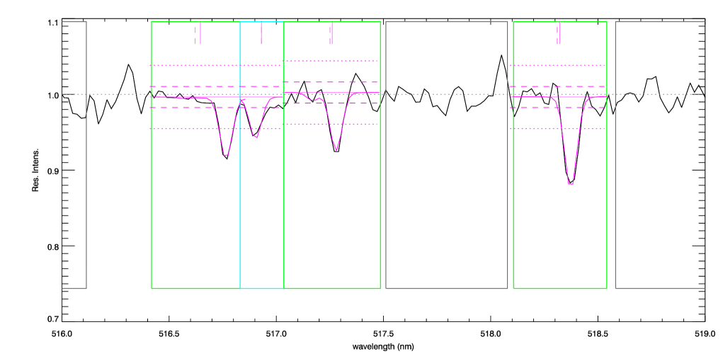
A summary of the stellar parameters of the sample of stars is available in Table 2. The chemical abundances for Fe, Si, Mg, and Ca were derived with the code MyGIsFOS (Sbordone et al. 2013), based on the OSMARCS-turbospectrum grid of synthetic spectra, and are shown in Table 3. The reference solar abundances are taken from Caffau et al. (2011a) for C and Fe, and from Lodders et al. (2009) for the other elements. An example of line fitting for the Mg i lines performed by MyGIsFOS is shown in Fig. 1.

Figure 1: Observed spectrum of SDSS J014828+150221 (solid black) in the region of the Mg ib triplet with the best fit superimposed (solid pink). The green boxes enclose the range for the fit on the Mg i lines, the light-blue box that for the fit on the Fe ii line. The magenta horizontal solid lines represent the continuum, the magenta horizontal dashed lines represent one $\sigma$ of the S/N ratio of the observed spectrum in the region, and the magenta horizontal dotted lines represent three $\sigma$ of the S/N ratio. The magenta vertical solid lines show the wavelength at the centre of the fitting range at rest, and the magenta vertical dashed lines show the same after the shift assumed by the fitting.

For iron, for which several lines can be detected, the $\sigma$ given in Table 3 and Fig. 4 is the line-to-line scatter. The same is true for the other elements for which more than one line can be detected. To estimate the error for elements for which only one line could be measured we computed Monte Carlo simulations of 1000 events on the Ca i line at 422.8 nm and on the Si i line at 390.5 nm, and derived a $\sigma$ of 0.19 Caffau et al. (2013). For the Monte Carlo simulation we injected a Poisson noise of 45 in a synthetic spectrum of parameters ($T\rm_{eff}$/$\log g$/[Fe/H]) 6200/4.0/–3.5 for the above mentioned lines and analysed them with MyGIsFOS.

We examined the G-band to detect CEMP stars. We derived an upper limit from 1D synthetic spectra and found no star on the C-plateau of Spite et al. (2013). For hot stars the upper limits are less significant because the band is weak. We know that the molecular bands are very sensitive to granulation effects (Bonifacio et al. 2013), therefore we plan to base the analysis of the G-band on hydrodynamical models for the complete sample of stars observed during the TOPoS survey.

The star SDSS J031348+011456 is on the hot side of the sample, therefore the lines appear weak in the spectrum, even though this is not one of the most metal-poor objects of the sample. The low S/N induces a high line-to-line scatter in the abundances.

For star SDSS J214633-003910, the Mg i line at 470.29 nm gives an abundance about 2 dex higher than the abundance derived from the other Mg lines. We have no explanation for this, but we removed this line from the analysis.

Typically, the calcium abundance derived from the Ca ii lines of the IR triplet is very high, on average by 0.4 dex higher than the abundance obtained from the Ca i lines. We are aware that the sky subtraction, when observing with the IFU, is difficult in the visible arm. In addition, the Ca triplet lines are affected by NLTE (Mashonkina et al. 2007) and granulation effects. Spite et al. (2012) derived NLTE corrections for the Ca triplet lines of about –0.4 dex for an effective temperature in the range of 6000-6500 K, a gravity of 4, and $[{\rm Fe/H}]=-3.5$. The specific problems affecting these lines will be addressed when the complete sample of stars is available.

Table 2: Stellar parameters and main results.

Star	${\rm T_{\rm eff}}$	$\log g$	$\xi$	S/N	[Fe/H]SDSS	[Fe/H]	A(C)
		K	$\mathrm{km\,s^{-1}}$	@ 400 nm
SDSS J000411-055027	6174	4.0	1.5	30	$-4.44$	$-2.96$	$\leq 6.5$
SDSS J002558-101509	6408	4.0	1.5	40	$-3.53$	$-3.08$	$\leq 6.5$
SDSS J014036+234458	5848	4.0	1.5	58	$-3.65$	$-3.83$	$\leq 6.0$
SDSS J014828+150221	6151	4.0	1.5	52	$-3.11$	$-3.41$	$\leq 6.0$
SDSS J031348+011456	6335	4.0	1.5	29	$-3.15$	$-3.31$	$\leq 7.0$
SDSS J040114-051259	5500	4.0	1.5	29	$-3.04$	$-3.62$	$\leq 5.0$
SDSS J105002+242109	5682	4.0	1.5	40	$-3.16$	$-3.93$	$\leq 6.2$
SDSS J112750-072711	6474	4.0	1.5	67	$-3.30$	$-3.34$	$<7.0$
SDSS J124121-021228	5672	4.0	1.5	57	$-3.04$	$-3.47$	$\leq 6.0$
SDSS J124304-081230	5488	4.0	1.5	40	$-3.17$	$-3.92$	$\leq 5.5$
SDSS J124719-034152	6332	4.0	1.5	73	$-3.41$	$-4.11$	$\leq 6.0$
SDSS J150702+005152	6555	4.0	1.5	40	$-4.46$	$-3.51$	$\leq 7.0$
SDSS J172552+274116	6624	4.0	1.5	30	$-3.22$	$-2.91$	$\leq 7.0$
SDSS J214633-003910	6475	4.0	1.5	64	$-3.12$	$-3.14$	$\leq 6.5$
SDSS J220121+010055	6392	4.0	1.5	49	$-3.54$	$-3.03$	$\leq 6.5$
SDSS J222130+000617	5891	4.0	1.5	25	$-3.48$	$-3.14$	$\leq 6.0$
SDSS J225429+062728	6169	4.0	1.5	26	$-3.52$	$-3.01$	$\leq 5.5$
SDSS J230243-094346	5861	4.0	1.5	43	$-5.55$	$-3.71$	$\leq 5.5$
SDSS J235210+140140	6313	4.0	1.5	54	$-3.30$	$-3.54$	$\leq 6.0$

Table 3: Abundances

Star	[Fe i/H]	$\sigma$	N	[Fe ii/H]	$\sigma$	N	[Mg/H]	$\sigma$	N	[Si/H]	N	[Ca i/H]	$\sigma$	N	[Ca ii/H]	$\sigma$	N
SDSS J000411-055027	$-2.96$	0.32	13				$-2.42$	0.38	5			$-3.33$		1	$-2.43$	0.13	2
SDSS J002558-101509	$-3.08$	0.23	14				$-2.89$	0.18	5			$-3.20$		1	$-2.02$	0.31	3
SDSS J014036+234458	$-3.83$	0.21	27				$-3.38$	0.21	4	$-3.82$	1	$-3.78$		1	$-3.20$	0.13	3
SDSS J014828+150221	$-3.41$	0.22	25	$-3.17$		1	$-3.26$	0.18	3			$-3.88$		1	$-2.71$	0.34	2
SDSS J031348+011456	$-3.31$	0.42	6									$-3.10$		1	$-2.79$		1
SDSS J040114-051259	$-3.69$	0.36	7				$-3.56$	0.20	3	$-3.42$	1	$-3.18$		1
SDSS J105002+242109	$-3.93$	0.27	11	$-3.49$		1	$-2.99$	0.05	3	$-3.43$	1	$-3.98$		1	$-2.95$	0.09	2
SDSS J112750-072711	$-3.34$	0.30	17				$-3.13$	0.09	3			$-3.38$		1	$-1.94$		1
SDSS J124121-021228	$-3.47$	0.22	40	$-3.39$		1	$-2.95$	0.11	5	$-3.35$	1	$-3.99$		1	$-2.79$		1
SDSS J124304-081230	$-3.92$	0.28	24				$-3.40$	0.23	5	$-3.36$	1	$-3.73$		1	$-2.95$	0.04	3
SDSS J124719-034152	$-4.11$	0.18	11				$-3.55$	0.30	3			$-3.96$		1	$-2.78$	0.13	2
SDSS J150702+005152	$-3.51$	0.17	7				$-3.05$	0.21	4						$-2.33$	0.11	3
SDSS J172552+274116	$-2.91$	0.38	6				$-2.89$	0.20	4			$-3.29$		1	$-2.31$	0.14	3
SDSS J214633-003910	$-3.14$	0.28	30	$-3.24$		1	$-2.91$	0.20	4	$-3.56$	1	$-3.11$		1	$-2.47$	0.29	3
SDSS J220121+010055	$-3.03$	0.23	23	$-3.04$	0.15	2	$-2.62$	0.17	5	$-3.77$	1	$-3.25$		1	$-2.00$	0.21	3
SDSS J222130+000617	$-3.14$	0.15	10				$-3.17$	0.14	2						$-2.83$	0.20	2
SDSS J225429+062728	$-3.01$	0.30	10				$-2.54$	0.36	2			$-3.28$		1	$-2.05$	0.03	3
SDSS J230243-094346	$-3.71$	0.27	14				$-3.32$	0.19	5	$-3.61$	1				$-3.47$	0.14	2
SDSS J235210+140140	$-3.54$	0.26	13				$-2.94$	0.25	4	$-3.57$	1				$-2.16$	0.14	3

7 Kinematics

We performed a preliminar analysis of the kinematic properties of the two stars with the most extreme radial velocities. A more extended evaluation is deferred to a forthcoming paper on the kinematics of the TOPOS stars. The stars are SDSS J112750-072711 and SDSS J014828+150221, which have a radial velocity of $419$$\mathrm{km\,s^{-1}}$ and $-411$$\mathrm{km\,s^{-1}}$, respectively, with an uncertainty of $\simeq 10$$\mathrm{km\,s^{-1}}$.

We calculated the orbital solutions using a standard Allen & Santillan (1991) model, after obtaining the distance of each star by fitting the SDSS photometry with a set of metal-poor 13 Gyr old isochrones from Girardi et al. (2004). Since the colours of the stars are compatible with either main sequence (MS), sub-giant branch (SGB), or horizontal branch (HB) stars, we adopted the distance for the MS star. The distance from the Sun of both stars is approximately $\sim 4$ kpc. For both stars we have at our disposal two estimates for the proper motion: one from the SDSS DR9, and one from PPMXL (Roeser et al. 2010). Although the values for each star are compatible within errors (the reference datasets are the same), we decided to explore all possible orbital solutions on a grid of $-40\div+40$ mas/yr in both RA and DEC, keeping ${\rm v}_{\rm rad}$ and distance fixed. This allowed us to reach a more reliable conclusion on the real solution given the high uncertainties of the proper motions. For both stars we computed the eccentricity of the orbit starting from the orbital solution, not from the proper motion. This computation provides a better intrinsic shape of the orbit than the kinetatic value.

We found that star SDSS J112750-072711 is on a highly radial orbit with an eccentricity of $\sim 0.97$ and a minimum radial distance of $\sim 6$ kpc: the star is actually approaching its minimum orbital radial distance. The maximum radial orbital distance varies from a lower value of $\sim 85$ kpc for a zero value of the proper motion to values higher than 200 kpc in the case of proper motions larger than $\sim 10$ mas/yr, as are indeed measured. We can consider a star with such a large maximum radial orbital distance a real outer halo object, loosely connected with the Milky Way and possibly belonging to some external galaxy.

The conclusions are similar for star SDSS J014828+150221. The orbit is quite radial with an eccentricity of $\sim 0.90$ and a minimum radial distance of $\sim 6$ kpc. ${\rm R}_{\rm MAX}$ varies from $80$ kpc to more than 200 for a proper motion of $\sim 12$ mas/yr. Considering that for this star the estimated proper motion is $\sim 4$ mas/yr, it is more probable that this star is an outer halo star.

The extreme radial velocity is a clear signature that these stare are outer halo members. If the high proper motion is confirmed for SDSS J112750-072711 we can consider this as an extragalactic star at its first visit to the Milky Way.

8 Discussion

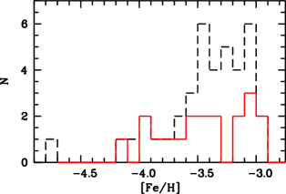
We analysed a sub-sample of EMP stars observed during the Large Programme TOPoS. The selection was set with the aim to find the most metal-poor TO stars, but we also selected relatively bright stars for X-Shooter to calibrate the Galactic MDF. For this sample of 19 stars, [Fe/H] ranges from $-4.1$ to $-2.9$ and the average value is $-3.32$. In Fig. 2 we show the metallicity histogram for this sample of stars. We found no evidence for a drop at [Fe/H]=–3.5 in contrast to the results of Schörck et al. (2009), although we note that this result was already expected from the figure 3 of Ludwig et al. (2008). There is a disagreement between [Fe/H] we derive from X-Shooter spectra and the metallicity we derive from SDSS spectra of up to about 2 dex, as can also be seen from figure 5 of Caffau et al. (2011c), especially for the lowest metallicity. We recall that the metallicity derived from SDSS spectra is often based on the lines of $\alpha$ elements (e.g. the Mg ib triplet) and in some cases only on the Ca ii-K line, which can be contaminated by a substantial contribution by the inter-stellar component. The analysis of X-Shooter spectra allows us to derive [Fe/H], [$\alpha$/Fe], and usually also a useful upper limit on the carbon abundance.

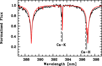
Of the 19 stars analysed, one has $[{\rm Fe/H}]<-4$ (SDSS J124719-034152). In Fig. 3 its wavelength range around the Ca ii H and K lines is shown. For seven stars $-4<[{\rm Fe/H}]<-3.5$. From the present small sample it is clear that there is no cut-off in the MDF at $[{\rm Fe/H}]\approx-3.5$, because eight stars lie below this value. We can confirm the low metallicity of all the stars, but we have not yet found another extreme object like SDSS J102715+172927 (Caffau et al. 2011b). SDSS J102715+172927 was selected with five other objects and happened to be an outlier. Statistically, we could expect another star of this type in a sample of 19 stars. However, it can be misleading to assamble statistics from such small numbers, but it may be that EMP stars not enhanced in carbon, with $[{\rm Fe/H}]<-4.5$, are extremely rare, and much lower in number than CEMP stars with the same limit in iron.

Figure 2: The histogram of the metallicities for this sample of stars (solid red) compared to the one (1D-LTE [Fe/H] value) from our complete sample of stars (dashed red) selected from SDSS and observed with X-Shooter (Caffau et al. 2011c; Caffau et al. 2012) and UVES (Bonifacio et al. 2012).

Figure 3: Spectrum of SDSS J124719-034152 in the range of the Ca ii-H and -K lines (solid black) compared with a synthetic spectrum of metallicity $-4$ (solid red). The Ca stellar lines are marked with a solid black line, the interstellar components with a dashed black line.

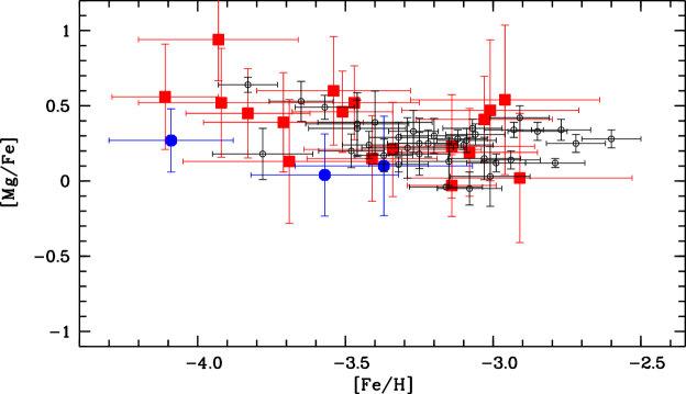
The most suitable element for investigating in the $\alpha$-enhancement in our sample of stars is Mg, because the Mgb triplet falls in the UVB range as well as some other Mg i lines. In Fig. 4, [Mg/Fe] vs. [Fe/H] is compared with that of other EMP stars. As stated in Caffau et al. (2013) (filled blue circles, in Fig.4), where we discussed two EMP stars low in $\alpha$, [Mg/Fe] shows a large scatter and several stars show a low value. The two halo objects with high radial velocity discussed in Sec. 7 are not extremely low in [Mg/Fe] (+0.15 and +0.21 for SDSS J014828+150221 and SDSS J112750-072711, respectively). A more reliable statement will be possible with the complete sample and after appropriate NLTE and 3D computations. It is possible that a part of the scatter seen in the present analysis is due to the neglect of 3D and NLTE effects.

Figure 4: [Mg/Fe] vs. [Fe/H] diagram for the programme stars (filled red squares) compared with the three stars analysed in Caffau et al. (2013) (filled blue hexagons) and those in the samples of Bonifacio et al. (2009) and Bonifacio et al. (2012) (black open circle).

[x]lrrr Atomic lines.
Element $\lambda$ ${\rm E}_{\rm low}$ log gf
[nm] [eV]
continued.
Element $\lambda$ ${\rm E}_{\rm low}$ log gf
[nm] [eV]
Mg i 382.9355 2.709 $-0.231$
Mg i 383.2299 2.712 $-0.356$
Mg i 383.2304 2.712 $+0.021$
Mg i 383.8292 2.717 $+0.392$
Mg i 383.8295 2.717 $-0.335$
Mg i 383.8290 2.717 $-1.530$
Mg i 470.2991 4.346 $-0.666$
Mg i 516.7321 2.709 $-0.931$
Mg i 517.2684 2.712 $-0.450$
Mg i 518.3604 2.717 $-0.239$
Si i 390.5523 1.909 $-0.743$
Ca i 422.6728 0.000 $+0.265$
Ca i 443.4957 1.886 $-0.007$
Ca i 445.4779 1.899 $+0.335$
Ca ii 393.3663 0.000 $+0.105$
Ca ii 849.8023 1.692 $-1.469$
Ca ii 854.2091 1.700 $-0.514$
Ca ii 866.2141 1.692 $-0.770$
Fe i 355.4924 2.832 $+0.538$
Fe i 355.6878 2.851 $-0.040$
Fe i 355.8515 0.990 $-0.629$
Fe i 356.5379 0.958 $-0.133$
Fe i 356.5582 2.865 $-0.496$
Fe i 357.0098 0.915 $+0.153$
Fe i 357.0254 2.808 $+0.728$
Fe i 358.1193 0.859 $+0.406$
Fe i 360.8859 1.011 $-0.100$
Fe i 364.7843 0.915 $-0.194$
Fe i 370.7822 0.087 $-2.407$
Fe i 370.7920 2.176 $-0.466$
Fe i 370.9246 0.915 $-0.646$
Fe i 371.9935 0.000 $-0.431$
Fe i 372.7619 0.958 $-0.631$
Fe i 374.3362 0.990 $-0.785$
Fe i 374.3468 3.573 $+0.146$
Fe i 374.5561 0.087 $-0.771$
Fe i 374.5899 0.121 $-1.335$
Fe i 375.8233 0.958 $-0.027$
Fe i 376.3789 0.990 $-0.238$
Fe i 376.5539 3.237 $+0.482$
Fe i 376.7192 1.011 $-0.390$
Fe i 378.7880 1.011 $-0.860$
Fe i 379.0093 0.990 $-1.761$
Fe i 379.5002 0.990 $-0.761$
Fe i 381.2964 0.958 $-1.047$
Fe i 381.5840 1.485 $+0.237$
Fe i 382.0425 0.859 $+0.119$
Fe i 382.4444 0.000 $-1.362$
Fe i 382.5881 0.915 $-0.037$
Fe i 382.7822 1.557 $+0.062$
Fe i 384.0437 0.990 $-0.506$
Fe i 384.1048 1.608 $-0.045$
Fe i 384.9966 1.011 $-0.871$
Fe i 385.0818 0.990 $-1.734$
Fe i 385.6371 0.052 $-1.286$
Fe i 385.9911 0.000 $-0.710$
Fe i 386.5523 1.011 $-0.982$
Fe i 387.2501 0.990 $-0.928$
Fe i 387.8573 0.087 $-1.379$
Fe i 387.8018 0.958 $-0.914$
Fe i 388.6282 0.052 $-1.076$
Fe i 388.7048 0.915 $-1.144$
Fe i 389.5656 0.110 $-1.670$
Fe i 389.8009 1.011 $-2.018$
Fe i 389.7890 2.692 $-0.736$
Fe i 389.9707 0.087 $-1.531$
Fe i 390.2945 1.557 $-0.466$
Fe i 390.6479 0.110 $-2.243$
Fe i 392.0258 0.121 $-1.746$
Fe i 392.2912 0.052 $-1.651$
Fe i 392.7920 0.110 $-1.522$
Fe i 393.0297 0.087 $-1.491$
Fe i 400.5242 1.557 $-0.610$
Fe i 404.5812 1.485 $+0.280$
Fe i 406.2441 2.845 $-0.862$
Fe i 407.1738 1.608 $-0.022$
Fe i 413.2058 1.608 $-0.675$
Fe i 414.3868 1.557 $-0.511$
Fe i 414.3415 3.047 $-0.204$
Fe i 418.1755 2.831 $-0.371$
Fe i 418.7795 2.425 $-0.554$
Fe i 418.7039 2.449 $-0.548$
Fe i 420.2029 1.485 $-0.708$
Fe i 423.5936 2.425 $-0.341$
Fe i 425.0787 1.557 $-0.714$
Fe i 425.0119 2.469 $-0.405$
Fe i 426.0474 2.399 $-0.109$
Fe i 427.1760 1.485 $-0.164$
Fe i 427.1153 2.449 $-0.349$
Fe i 428.2403 2.176 $-0.779$
Fe i 430.7902 1.557 $-0.073$
Fe i 432.5762 1.608 $+0.006$
Fe i 437.5930 0.000 $-3.031$
Fe i 438.3545 1.485 $+0.200$
Fe i 440.4750 1.557 $-0.142$
Fe i 441.5122 1.608 $-0.615$
Fe i 442.7310 0.052 $-2.924$
Fe i 446.1653 0.087 $-3.210$
Fe i 446.6551 2.831 $-0.600$
Fe i 447.6019 2.845 $-0.819$
Fe i 448.2170 0.110 $-3.501$
Fe i 449.4563 2.198 $-1.136$
Fe i 452.8614 2.176 $-0.822$
Fe i 489.1492 2.851 $-0.111$
Fe i 489.0755 2.875 $-0.394$
Fe i 492.0502 2.832 $+0.068$
Fe i 491.8954 4.154 $-0.672$
Fe i 491.8994 2.865 $-0.342$
Fe i 495.7596 2.808 $+0.233$
Fe i 495.7298 2.851 $-0.407$
Fe i 495.7682 4.191 $-0.400$
Fe i 501.2068 0.859 $-2.642$
Fe i 522.7189 1.557 $-1.228$
Fe i 526.9537 0.859 $-1.327$
Fe i 527.0356 1.608 $-1.339$
Fe i 532.8039 0.915 $-1.466$
Fe i 532.8531 1.557 $-1.850$
Fe i 537.1489 0.958 $-1.645$
Fe i 542.9696 0.958 $-1.879$
Fe ii 492.3927 2.891 $-1.504$
Fe ii 501.8440 2.891 $-1.100$
Fe ii 516.9033 2.891 $-1.000$