Effect of gravitational stratification on the propagation of a CME

Abstract

Context. Coronal mass ejections (CMEs) are the most violent phenomenon found on the Sun. One model that explains their occurrence is the flux rope ejection model. A magnetic flux rope is ejected from the solar corona and reaches the interplanetary space where it interacts with the pre-existing magnetic fields and plasma. Both gravity and the stratification of the corona affect the early evolution of the flux rope.

Aims. Our aim is to study the role of gravitational stratification on the propagation of CMEs. In particular, we assess how it influences the speed and shape of CMEs and under what conditions the flux rope ejection becomes a CME or when it is quenched.

Methods. We ran a set of MHD simulations that adopt an eruptive initial magnetic configuration that has already been shown to be suitable for a flux rope ejection. We varied the temperature of the backgroud corona and the intensity of the initial magnetic field to tune the gravitational stratification and the amount of ejected magnetic flux. We used an automatic technique to track the expansion and the propagation of the magnetic flux rope in the MHD simulations. From the analysis of the parameter space, we evaluate the role of gravitational stratification on the CME speed and expansion.

Results. Our study shows that gravitational stratification plays a significant role in determining whether the flux rope ejection will turn into a full CME or whether the magnetic flux rope will stop in the corona. The CME speed is affected by the background corona where it travels faster when the corona is colder and when the initial magnetic field is more intense. The fastest CME we reproduce in our parameter space travels at $\sim 850$ $km/s$. Moreover, the background gravitational stratification plays a role in the side expansion of the CME, and we find that when the background temperature is higher, the resulting shape of the CME is flattened more.

Conclusions. Our study shows that although the initiation mechanisms of the CME are purely magnetic, the background coronal plasma plays a key role in the CME propagation, and full MHD models should be applied when one focusses especially on the production of a CME from a flux rope ejection.

1 Introduction

Coronal mass ejections (CMEs) are the main drivers of space weather, a term used to describe the effect of plasmas and magnetic fields on the near Earth environment. Although the precise mechanism that causes a CME on the Sun is still unclear, the ejection of a magnetic flux rope from the solar corona successfully describes many of the general features of CMEs (Forbes & Isenberg (1991), Amari et al. (2000), Fan & Gibson (2007)). After the ejection of the magnetic flux rope, the CME propagates through the solar corona and into interplanetary space. Understanding CME propagation is a key element in space weather.

A key characteristic of a CME is the three-part structure (Hundhausen, 1987). A CME is normally composed of a dense bow front, followed by a low-density region and, finally, a very dense core placed approximately at the centre of the curved front. The propagation of this structure is normally used to infer the trajectory and speed of the CME. Several studies have analysed the kinematics of CMEs, and quoted speeds span from 100 km/s to 3300 km/s, with an average speed of about 500 km/s (Gopalswamy, 2004). Some CMEs undergo an impulsive acceleration phase followed by a propagation at constant speed (Zhang et al., 2001), while others are subject to relatively long acceleration (Chen & Krall, 2003). While CMEs may propagate at different speeds, all CMEs eventually couple with the solar wind once they reach a height of about $4$ $R_{\odot}$ (Gopalswamy et al., 2000). Similarly, CMEs expand while travelling outward (Ciaravella et al. (2001), Lee et al. (2009)).

As CMEs propagate in the solar corona they interact with the pre-exsiting plasma and magnetic fields. The solar corona is a highly dynamic environment composed of magnetized plasma whose global physical evolution can be described by magnetohydrodynamics (MHD) theory. In the solar corona, plasma motions are primarily driven by the Lorentz force. However, under equilibrium conditions we can assume a zero Lorentz force acting on the plasma. In such cases, the plasma distribution in the corona can be described as being stratified by the effect of gravity. The solar corona is inherently a multi-temperature environment, although highly efficient thermal conduction tends to thermalize the plasma, especially in the quiet corona.

The ratio between the thermal and magnetic pressure, the $\beta$ of the plasma determines whether the local dynamics is governed by the magnetic field ($\beta<1$) or the plasma ($\beta>1$). Gary (2001) describes the $\beta$ distribution in the corona and shows that in the lower corona, $\beta<1$. In contrast in the outer corona, the $\beta$ value has a more diversified distribution where $\beta<1$ regions alternate with regions where $\beta>1$. Moreover, when a CME occurs, it carries outward plasma and magnetic flux, which compress the plasma and magnetic field ahead of it, thereby changing the $\beta$ profile. Despite this interaction, it is important to note that the closed magnetic field of the ejected plasmoid allows neither the mixing nor thermalization of the ejected plasma with the surrounding corona (Ciaravella et al. (2001), Pagano et al. (2007)).

Thermal pressure is generally considered to play no role in the initial stages of the ejection of the flux rope, but does become relevant during the propagation phase of the CME when the flux rope travels at large radial distances. Similarly, gravity tends to obstruct the ejection, although it can significantly affect only fragments of the eruption. Innes et al. (2012) observed fragments of the eruption falling back to the Sun after an eruption.

Here we specifically address the role of gravitational stratification on the CME propagation. In our framework, the ejection is caused by an magnetic field configuration where the Lorentz force is not zero. This magnetic field is added to the stratified solar corona, which is initially in hydrostatic equilibrium and decoupled from the magnetic field. In particular, we start from the model of Pagano et al. (2013) where an eruptive magnetic configuration is used, and the full life span of a magnetic flux rope is described by coupling the global non-linear force free model of Mackay & van Ballegooijen (2006) with MHD simulations run with the AMRVAC code (Keppens et al., 2012). In Pagano et al. (2013) a rather simple background density and thermal pressure profile allowed a detailed study of the dynamics of the ejection. Here, we extend that model to include solar gravity and density stratification in the initial conditions. We explore how the parameter space affects the eruption characteristics by tuning both the temperature of the solar corona and the intensity of the magnetic field.

Several studies have included density stratification and gravity in CME modelling and propagation. Pagano et al. (2007) study the role of the ambient magnetic field topology in the CME expansion and thermal insulation, Zuccarello et al. (2009) focus on the CME initiation mechanisms including gravity and the solar wind. Archontis et al. (2009) describe a flux rope ejection in the presence of gravity following a magnetic flux emergence event. Finally, Manchester et al. (2004) model a CME considering the solar wind and gravity up to 1 AU, while Reeves et al. (2010) simulate a solar eruption in 2.5D including solar gravity and the effects of thermal conduction, radiation, and coronal heating. Moreover, Roussev et al. (2012) study solar eruptions with a treatment of thermodynamics and an eruption initiated from below the corona, while the effect of solar wind heating has recently been studied by Pomoell & Vainio (2012).

Although many observations have focussed on studying the properties of CMEs, studies that simultaneously consider the density stratification, and the ejected plasma and magnetic flux are difficult, owing the complexity of the different diagnostics involved. Some recent work that describes the propagation of CMEs in the solar corona include Gopalswamy et al. (2012) and Bemporad et al. (2011). Other studies give diverse examples of how the CME propagation can be modified according to the environment where it develops; e.g., Temmer et al. (2012) describe the interaction of a CME with another CME that preceded it. Separately, some studies have been carried out to analyse the consequence of the gravitational stratification of the solar corona (Guhathakurta et al. (1999), Antonucci et al. (2004), Verma et al. (2013)). As observational studies are difficult to carry out, our simulations will shed some light on physical problems that are still difficult to investigate from an observational view point.

The paper is structured as follows. In Sect.2, we describe the numerical model, in Sect.3 we describe the results of our simulations, in Sect.4 we discuss the results, and the conclusions are drawn in Sect.5.

2 Model

To study the effect of gravitational stratification on the propagation of a CME, we start from the work of Pagano et al. (2013) where a magnetic configuration has been shown to be suitable for ejecting a magnetic flux rope. In the present work, we perform a number of changes to the modelling technique of Pagano et al. (2013), in order to focus on the role of gravitational stratification. We have carried out a set of MHD simulations that consider variations in the temperature of the background coronal atmosphere and the magnetic field intensity.

2.1 MHD simulations

We used the AMRVAC code developed at the KU Leuven to run the simulations (Keppens et al., 2012). The code solves the MHD equations, and the terms that account for gravity are included:

$$\frac{\partial\rho}{\partial t}=-\@vec{\nabla}\cdot(\rho\@vec{v}),$$ (1)

$$\frac{\partial\rho\@vec{v}}{\partial t}+\@vec{\nabla}\cdot(\rho\@vec{v}\@vec{v})=-\nabla p+\frac{(\@vec{\nabla}\times\@vec{B})\times\@vec{B})}{4\pi}+\rho\@vec{g},$$ (2)

$$\frac{\partial\@vec{B}}{\partial t}=\@vec{\nabla}\times(\@vec{v}\times\@vec{B}),$$ (3)

$$\frac{\partial e}{\partial t}+\@vec{\nabla}\cdot[(e+p)\@vec{v}]=\rho\@vec{g}\cdot\@vec{v},$$ (4)

where $t$ is the time, $\rho$ the density, $\@vec{v}$ velocity, $\@vec{B}$ magnetic field, and $p$ thermal pressure. The total energy density $e$ is given by

$$e=\frac{p}{\gamma-1}+\frac{1}{2}\rho\@vec{v}^{2}+\frac{\@vec{B}^{2}}{8\pi}$$ (5)

where $\gamma=5/3$ denotes the ratio of specific heats. The expression for the solar gravitational acceleration is

$$\@vec{g}=-\frac{GM_{\odot}}{r^{2}}\hat{r},$$ (6)

where $G$ is the gravitational constant, and $M_{\odot}$ denotes the mass of the Sun. In order to gain accuracy in the description of the thermal pressure, we make use of the magnetic field splitting technique (Powell et al., 1999), as explained in Sect. 2.3 of Pagano et al. (2013).

The initial magnetic field condition of the simulations is chosen such that it initially produces the ejection of a flux rope and so the subsequent CME propagation can be studied. The configuration of the magnetic field is Day 19 in the simulation of Mackay & van Ballegooijen (2006). Pagano et al. (2013) in Sect. 2.2 explain in detail how the magnetic field distribution is imported from the global non-linear force free field (GNLFFF) model of Mackay & van Ballegooijen (2006) to our MHD simulations. Since the GNLFFF model contains no plasma, it needs to be defined. We assume an initial atmosphere of a constant temperature corona stratified by solar gravity, where we also allow for low background pressure and density:

$$\rho(r)=\rho_{0}e^{{\frac{M_{\odot}G\mu m_{p}}{Tk_{b}r}}}+\rho_{bg},$$ (7)

$$p(r)=\frac{k_{b}T}{\mu m_{p}}\rho_{0}e^{{\frac{M_{\odot}G\mu m_{p}}{Tk_{b}r}}}+p_{bg}$$ (8)

where we use $\rho_{0}$ to tune the density at the lower boundary, $\mu=1.31$ is the average particle mass in the solar corona, $m_{p}$ is the proton mass, $k_{b}$ Boltzmann constant, and $T$ the temperature of the corona. We tune $\rho_{0}$ depending on the temperature $T$ in order to always have the same density at the bottom of our computational domain. When $\rho_{bg}=p_{bg}=0$, we have a stratified atmosphere in hydrostatic equilibrium. In some simulations, we need to have non-zero values for $\rho_{bg}$ and $p_{bg}$ to avoid extremely low $\beta$ values at the outer radial boundary of the simulation. These values are chosen such that $p_{bg}=\rho_{bg}/(\mu m_{p})k_{b}T$. In our simulations such a departure from equilibrium implies a negligible inflow of plasma (in contrast to the real solar corona that is outflowing). More details are given in the Appendix. Finally, we set $\@vec{v}=0$ as initial condition for the velocity.

Since the results of Mackay & van Ballegooijen (2006) are specified in terms of the potential vector $\@vec{A}$, we can uniformly multiply our initial magnetic field distribution without hindering the validity of the results of Mackay & van Ballegooijen (2006). In the present work, we use the maximum value of the magnetic field intensity of the initial magnetic field configuration, $B_{max}$, as a simulation parameter. In our simulation, the magnetic field intensity is maxmium, $|B|=B_{max}$, at the centre of the right-hand side bipole on the lower boundary.

The simulation domain extends over $3$ $R_{\odot}$ in the radial dimension starting from $r=R_{\odot}$. The colatitude, $\theta$, spans from $\theta=30^{\circ}$ to $\theta=100^{\circ}$ and the longitude, $\phi$, spans over $90^{\circ}$. This domain extends to a larger radial distance than the domain used in Mackay & van Ballegooijen (2006) from which we import the magnetic configuration. To define the MHD quantities in the portion of the domain from $2.5$ $R_{\odot}$ to $4$ $R_{\odot}$, we use Eqs.7 and 8 for density and thermal pressure and the magnetic field for $r>2.5$ $R_{\odot}$ is assumed to be purely radial ($B_{\theta}=B_{\phi}=0$) where the magnetic flux is assumed to be conserved

$$B_{r}(r>2.5R_{\odot},\theta,\phi)=B_{r}(2.5R_{\odot},\theta,\phi)\frac{2.5^{2}}{r^{2}}.$$ (9)

It should be noted that the initiation of the ejection is not affected in any way by the extension of the magnetic field, since the initial dynamics are a result of the flux rope that lies at about $1.2$ $R_{\odot}$ out of magnetohydrostatic equilibrium.

The boundary conditions are treated with a system of ghost cells. Open boundary conditions are imposed at the outer boundary, reflective boundary conditions are set at the $\theta$ boundaries, and the $\phi$ boundaries are periodic. The $\theta$ boundary condition is designed to not allow any plasma or magnetic flux through, while the $\phi$ boundary conditions allow the plasma and magnetic field to freely evolve across the boundaries. These boundary conditions match those used in Mackay & van Ballegooijen (2006). In our simulations, the expanding and propagating flux rope only interacts with the $\theta$ and $\phi$ boundaries near the end of the simulations, thus they do not affect our main results regarding the initiation and propagation of the CME. At the lower boundary, we impose constant boundary conditions taken from the first four $\theta$-$\phi$ planes of cells derived from the GNLFFF model. The computational domain is composed of $256\times 128\times 128$ cells distributed in a uniform grid. Full details of the grid can be found in Sect. 2.3 of Pagano et al. (2013).

2.2 Parameter space investigation

To analyse the role of the background stratified corona we ran a set of nine simulations using three different temperatures ($T=1.5$,$2$,$3$ $MK$) of the corona and three different maximum intensity values of the magnetic field ($B_{max}=7$,$21$,$42$ $G$), as illustrated in Fig.1.

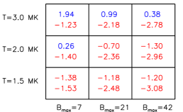
Figure 1: Grid summarizing the parameter space we investigate. We ran 9 simulations with all the combinations of $T=1.5$,$2$,$3$ $MK$ with $B_{max}=7$,$21$,$42$ $G$. The numbers in the cell represent the $Log_{10}(\beta)$ at the lower boundary (lower number) and the $Log_{10}(\beta)$ at the upper boundary (higher number). Red are negative values, and blue positive ones.

In our model, a higher corona temperature implies a more uniform density and pressure gradient from the photosphere to the outer corona and a higher amount of mass that constitutes the solar corona, as in Fig.2a. At the same time, the higher temperature leads to remarkably higher $\beta$ in the outer corona, as shown in Fig. 2b for the $B_{max}=7$ $G$ case, while in the lower corona ($r<1.2R_{\odot}$) $\beta$ is clearly below $\sim 10^{-1}$ regardless of the temperature. For the $B_{max}=21$ and $42$ $G$ cases, the $\beta$ value is lower. The outer corona switches from a low to a high $\beta$ regime when the temperature increases from $1.5$ to $3$ $MK$ (Fig.2b).

We use the temperature to define a part of the parameter space since it is the appropriate parameter to consistently tune the profile of density and thermal pressure in the solar corona. Since we always assume the same value for the photospheric density, an increase in temperature implies a heavier column of mass placed above the magnetic flux rope. By computing the integral of Eq.7 from $r=1.12$ $R_{\odot}$ to $r=4$ $R_{\odot}$, we get a column of mass of $7.5\times 10^{-6}$ $g/cm^{2}$ above the flux rope for the simulation with $T=1.5$ $MK$ and $25$ times more for the simulation with $T=3$ $MK$.

At the same time, the pressure scale height reduces when lower temperatures are considered. This implies that the ejected flux rope encounters less resistance from the compression produced ahead when propagating. The pressure length scale is around $0.06$ $R_{\odot}$ when the temperature is $T=1.5$ $MK$, which doubles to $0.12$ $R_{\odot}$ when the temperature is $T=3$ $MK$. It should be clarified, however, that in our simplified model for the gravitational stratification, we do not aim to realistically describe the entire multi-temperature structure of the solar corona, but rather the corona surrounding an active region. In all of the simulations, the density and pressure drop steeply in comparison to the full extent of the computational domain out to $4$ $R_{\odot}$.

Figure 2: (a) Profiles of $Log_{10}(\rho)$ along $r$ above the centre of the LHS bipole for different temperatures of the solar corona, $T$. (b) Profiles of $Log_{10}(\beta)$ along $r$ above the centre of the LHS bipole for different temperatures of the solar corona, $T$, and with $B_{max}=7$ $G$. (c) profiles of $Log_{10}(\beta)$ along $r$ above the centre of the LHS bipole with different values of the parameter $B_{max}$ and with $T=2$ $MK$

Simulations with different $B_{max}$ (Fig.2c) basically differ in the plasma $\beta$, which uniformly decreases as $B_{max}$ increases. Thus, by changing the parameter $B_{max}$ we generally modify the dominant forces and subsequently the capacity of the solar corona to react to the flux rope ejection.

In some of the simulations ($T=1.5$ $MK$; $B_{max}=21$ and $B_{max}=42$ $G$), we use a non-zero $p_{bg}$ and $\rho_{bg}$ to avoid numerical problems due to extremely low $\beta$ at the external boundary. For these simulations, the background pressure and density are four orders of magnitude slower than the values near the lower boundary where the dynamics originate. The resulting pressure and density profile departs from the analytic hydrostatic equilibrium profile, but we point out that this can slow down the ejection only slightly, because more plasma has to be displaced as the CME propagates due to the background density ($\rho_{bg}$). However, the kinetic energy carried by the ejected plasma in the flux rope is much greater than the kinetic energy produced by these motions, and these effects can in no way produce artificial ejections. The tests described in the Appendix show that such departures from hydrostatic equilibrium only lead to appreciable effects on the magnetic configuration on much larger time scales than the one for the CME to escape the solar corona in the present simulations.

3 Results

The initial magnetic field configuration is identical in all of the simulations and it is chosen to produce the ejection of the magnetic flux rope due to an initial excess of the Lorentz force. Figure 3 shows the initial magnetic configuration common to all the simulations. The only difference from the one used in Pagano et al. (2013) is the larger extension of the domain in the radial direction. The flux rope that is about to erupt lies under the arcade system, and external magnetic field lines are shown above. Some of the external magnetic field lines belong to the external arcade. while others are open. A full description of the initial magnetic field configuration is given in Sect.3.1 of Pagano et al. (2013).

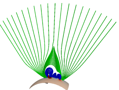
Figure 3: Magnetic field configuration used as the initial condition in all the MHD simulations. Red lines represent the flux rope, blue lines the arcades, green lines the external magnetic field. The lower boundary is coloured according to the polarity of the magnetic field from blue (negative) to red (positive) in arbitrary units.

In Pagano et al. (2013) the dynamics of the ejection and the production of the initial condition in the GNLFFF simulation is discussed in detail. Here, we only focus on the propagation of the flux rope once the ejection is triggered.

We first describe the characteristics of a typical ejection in this framework. Following this we compare some key features between different simulations in order to highlight the role of the temperature of the stratified corona ($T$) and the intensity of the magnetic field ($B_{max}$).

3.1 Typical simulation, ($T=2MK$, $B_{max}=21$ $G$)

A typical simulation is one with $T=2$ $MK$ and $B_{max}=21$ $G$, which is the central one in the parameter space grid shown in Fig.1. In this simulation the flux rope escapes the computational domain at $4$ $R_{\odot}$ and a CME occurs. In Fig.4 we show the ejection and expansion of the flux rope in 3D to illustrate the simulation with some of the magnetic field lines drawn from the flux rope footpoints and from the axis of the flux rope at different times. In future figures we draw cuts in 2D planes to focus more clearly on specific aspects.

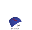
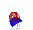
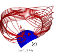
Figure 4: The ejection of the magnetic flux rope. The red lines are all magnetic flux rope lines draw from both the footpoints of the flux rope and from the centre of its axis.

In the initial magnetic configuration (Fig.3), the flux rope lies above the centre of the left-hand side (LHS) bipole, three magnetic arcades connect adjacent and opposite polarities, and a larger arcade connects the opposite external polarities of the two bipoles. The flux rope that is in non-equilibirium lies in the asymmetric part of the global configuration. The density profile falls off with radial distance where $\rho\sim 10^{-15}$ $g/cm^{3}$ at the lower boundary and $\rho\sim 10^{-20}$ $g/cm^{3}$ at the top boundary (Fig.2a). The plasma $\beta$ is approximately $10^{-2}$ near the flux rope and it increases to $10^{-1}$ radially above it (Fig.2c). We note that there are regions where $\beta$ reaches as much as $10^{2}$ in the corona (such as near null points), where the magnetic field is weak.

To follow the evolution of the simulation, in Fig.5 we show two quantities in the $r-\phi$ plane passing through the centre of the bipoles. Figures 5a-5c show the density contrast,

$$\rho_{c}=\frac{\rho(t)-\rho(t=0)}{\rho(t=0)},$$ (10)

that indicates the variation in density with respect to the initial condition, which is useful for marking the ejection of plasma. Figsures 5d-5f show the ratio $B_{\theta}/|B|$ that illustrates the evolution of the axial magnetic field of the flux rope, which initially lies in the $\theta$-direction. As explained in Mackay & van Ballegooijen (2006), the formation of the flux rope due to magnetic diffusion leads to a strong axial component of the magnetic field along the PIL of the LHS bipole. Simultaneously, the increased tilt of the bipole leads to a quasi-antiparallel magnetic field around the magnetic flux rope. Because of the construction of the system of a E-W bipole and N-S PIL, at $t=0$ the axial magnetic field of the flux rope is mostly along the $\theta$ direction and the blue region between pink and green in Figs. 5d-5f, across which $B_{\theta}/|B|$ changes sign, and then marks the borders of the magnetic flux rope and the overlying arcade. As long as no major reconnection occurs, the quantity $B_{\theta}/|B|$ is clearly positive above the bipoles where the magnetic flux rope propagates and expands.

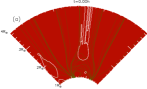
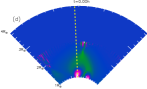
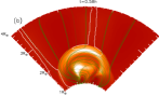
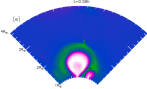
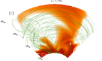
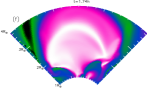
Figure 5: Simulation with $T=2$ $MK$ and $B_{max}=21$ $G$. (a)-(c) Maps of density contrast (Eq.10) in the $(r-\phi)$ plane passing through the centre of the bipoles at $t=0$h, $t=0.58$h, $t=1.74$h. Superimposed are magnetic field lines plotted from the same starting points (green lines) and the contour line of $\beta=1$ (white line). (d)-(f) Maps of $B_{\theta}/|B|$ on the same plane and at the same times. Maps show the full domain of our simulations from $r=1$ $R_{\odot}$ to $r=4$ $R_{\odot}$. In panel (d) the yellow dashed line is the cut for the plots in Fig.6. The temporal evolution is available in the on-line edition.

In this simulation, the flux rope is ejected outwards, and it leads to an increase in density at larger radii (Fig.5a-Fig.5c), and the propagation and expansion of the region where the magnetic field is mostly axial, i.e. $B_{\theta}/|B|\sim 1$ (Figs. 5c-5f). The shape of the density propagation roughly reproduces the typical three-component structure of a CME, which is clearly visible in Fig. 5b. A higher density bow front propagates upwards, and behind it lies a region with lower density. Finally, a dense core is located at the centre of the expanding dome. In our simulation, the region with highest density coincides with the region where $B_{\theta}/|B|$ is positive. The quantity $B_{\theta}/|B|$ is maximum just ahead of the high- density region, while the peak of density is highest roughly at the centre of the expanding structure where $B_{\theta}/|B|$ remains positive (Fig. 5b). This suggests that the magnetic flux rope is propagating upwards, perpendicular to its axial magnetic field lines, lifting coronal plasma to produce the high density region. The same process is seen in Pagano et al. (2013), and it is considered a standard process in filament eruptions.

At the same time, the region where a positive axial component of the magnetic field is dominant expands and propagates upwards, roughly covering the same volume of space as that of the high-density region (white and pink region in Figs. 5d-5f). Since the region where $B_{\theta}/|B|>0$ roughly reproduces the high- density region that corresponds to the CME, we use this quantity to track the ejection and expansion of the CME. Figure 6 shows the profile of $B_{\theta}/|B|$ radially from the centre of the LHS bipole at different times. The radial position where $B_{\theta}/|B|=0$ along the radial direction vertically from the centre of the LHS bipole is defined to be the top of the magnetic flux rope in our representation.

In the plot in Fig. 6 we see the top of the flux rope at $1.4$ $R_{\odot}$ at $t=0$h (black line), and it reaches $3.15$ $R_{\odot}$ after $1.16$h (red line). This clearly shows the ejection of the flux rope.

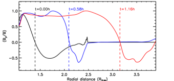
Figure 6: Profile of $B_{\theta}/|B|$ above the centre of the LHS bipole, at different times (different colours). Dashed lines of different colours indicate where $B_{\theta}/|B|=0$ and where we locate the top of the flux rope at a given time.

3.2 Parameter space investigation

3.2.1 Quenched ejections

Following the location of the top of the flux rope we are able to track the ejection of the flux rope and thus identify whether the flux rope ejection produces a CME (i.e. extends beyond $r=4$ $R_{\odot}$) or whether it is a quenched ejection. We find that the simulations with $T=2$ $MK$ and $T=3$ $MK$ where $B_{max}=7$ $G$ do not show any CME propagation. The flux rope only rises up to a given height and then stops. In Fig. 7, we show a quenched ejection for the simulation with $T=2$ $MK$ and $B_{max}=7$ $G$. In this simulation the magnetic flux rope is stopped and remains positioned at $r=1.8$ $R_{\odot}$ after $1.74$h.

A key difference between the simulation where a CME develops (Fig.5a) and where the ejection is quenched (Fig. 7a) is that a high-$\beta$ region lies above the flux rope in the simulation where the ejection is quenched. The fast CME can only develop in a low-$\beta$ environment. In particular, the $\beta=1$ contour overlies the flux rope in Fig. 7a, while it only surrounds the null-point region in Fig. 5a. Although this is not a necessary or sufficient condition to determine the onset of a full or quenched ejection, whether a high-$\beta$ region lies over the flux rope is one of the factors that can determine the CME evolution.

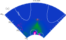
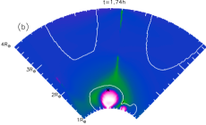
Figure 7: Simulation with $T=2$ $MK$ and $B_{max}=7$ $G$. Maps of $B_{\theta}/|B|$ in the $(r-\phi)$ plane passing through the centre of the bipoles at $t=0$h and $t=1.74$h. Superimposed is the contour line of $\beta=1$ (white line). Black crosses indicate where the top of the flux rope is positioned.

3.2.2 Parameter space of CMEs

All the remaining simulations show an ejection of the flux rope in a similar manner to the one in Sect. 3.1. We do not present a detailed analysis here for each simulation, but plot the position of the top of the flux rope as a function of time. In Fig. 8a we show the position of the top of the flux rope for the three simulations where $B_{max}=21$ $G$ (central column in Fig.1). We stop tracking the top of the flux rope as soon as it is close to the outer boundary and its propagation is affected by boundary effects. The speed quoted in Fig. 8 is the average speed of propagation. The average speed of the CME spans a wide range from $69$ $km/s$ to $498$ $km/s$. The lower the temperature, the faster the CME. Also, the CMEs propagating in a $2$ $MK$ or $1.5$ $MK$ corona are at near constant speed, while the speed varies slightly with radial distance for the slowest CME ($T=3$ $MK$).

Figure 8b shows the height of the top of the flux rope as a function of time for the three simulations with $T=2$ $MK$ (central row in Fig. 1). The higher the magnetic field ($B_{max}$), the stronger the initial force due to the unbalanced Lorentz force under the magnetic flux rope, and the CME travels faster. With $B_{\max}=7$ $G,$ we have a quenched ejection, while we have a $718$ $km/s$ fast CME with $B_{\max}=42$ $G$. By changing the parameter $B_{max}$, we change the Alfvén speed in the system and thus the evolution time scale. It should be noted that the result of the simulations with different $B_{max}$ cannot be inferred solely through timescale arguments owing to the presence of the plasma. For instance, this is demonstrated by the qualitatively different evolution of the simulation with $B_{\max}=7$ $G$ from the other simulations.

Figure 8: (a) Position of the top of the flux rope as a function of time in the three simulations with $B_{max}=21$ $G$. (b) Position of the top of the flux rope as function of time in the three simulations with $T=2$ $MK$.

We note that the speed of the top of the flux rope is not necessarily the speed of the CME. The top of the flux rope represents the leading edge of the CME, which is subjected to the combined effect of propagation and expansion. However, the results approximately indicate the speed of the CME and its dependence on the parameters $T$ and $B_{max}$. In Fig. 9 we summarize the speed of the CMEs for all of the simulations. The fastest CME in our simulations can reproduce speeds of $838$ $km/s$, and only two simulations show a quenched ejection.

Figure 9: Grid summarizing the average speed of the CME in the parameter space we investigate. Crosses indicate a quenched ejection, and in the other boxes we write the value of the CME speed computed from tracking the top of the flux rope as in Fig. 8.

We also use the quantity $B_{\theta}/|B|$ to follow the $\phi$ extension of the flux rope and thus its expansion. We draw the contour of the flux rope by tracking where the cut of $B_{\theta}/|B|$ along the $\phi$ direction on the $r$-$\phi$ plane passing through the centre of the bipoles changes sign at different radial distances. Then, we consider the maximum $\phi$ extension of the resulting flux rope contour. Figure 10a shows the extension of the flux rope as a function of the height of the top of the flux rope for the simulations where unquenched eruptions occur. In this plot we group the simulations by temperature with different colours. The intensity of the magnetic field $B_{max}$ does not significantly influence the expansion of the CME, i.e. its shape. This can be seen because lines with the same colour lie close to one another in Fig. 10a. In contrast, the background temperature, $T$, plays a significant role in shaping the ejection.

Below the height of $2$ $R_{\odot}$ the expansion proceeds in a similar manner for all the simulations. However, around this radial distance the simulations with $T=3$ $MK$ show a larger expansion for higher radii. In the simulations with $T=1.5$ $MK$ and $T=2$ $MK$, the expansion of the flux rope proceeds nearly uniformly until the flux rope touches the upper boundary where the extension is approximately $50^{\circ}$ and $70^{\circ}$, respectively. In contrast, in the simulations with $T=3$ $MK$, the expansion rate increases at about $2$ $R_{\odot}$, and the flux ropes covers an angle that is close to $80^{\circ}$ beyond $3$ $R_{\odot}$. At the height of $2.5$ $R_{\odot}$, the simulations with $T=3$ $MK$ show an expansion that is about twice as large as the expansion found in the simulations with a cooler stratified solar corona.

In summary, Fig. 10a shows that higher temperatures favour higher expansion of the CME, which in turn results in a flattened shape. The higher pressure and density above the ejecting flux rope slow down the radial propagation and favour the expansion of the CME towards the sides. An example of the different shape of the CME is given in Fig. 10b where we show a snapshot of the simulation with $T=3$ $MK$ and $B_{max}=21$ $G$ (to be compared with Fig. 5e).

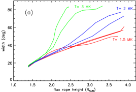
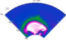
Figure 10: (a) Angular extension of the flux rope as a function of the radial distance of the top of the flux rope for all the simulations that show a CME. Simulations are grouped according to the simulation parameter $T$ given with different colours. (b) Map of $B_{\theta}/|B|$ in the $(r-\phi)$ plane passing through the centre of the bipoles at $t=1.55$h for the simulation with $T=3$ $MK$ and $B_{max}=21$ $G$. The map show the full domain of our simulations from $r=1$ $R_{\odot}$ to $r=4$ $R_{\odot}$.

4 Discussion

In this paper we have considered the role of gravitational stratification on the propagation of a CME. In order to do so, we investigated the parameter space by tuning the temperature of the corona (i.e. gravity stratification) and the maximum value of the magnetic field (i.e. the entire $\beta$ of the corona). The techniques and the initial magnetic configurations are identical to those of Pagano et al. (2013) where a CME initiation was successfully modelled.

4.1 Comparison with the flux rope ejection simulated in Pagano et al. (2013)

The purpose of the present work is not to analyse the mechanism that initiates the flux rope ejection in detail, since it does not show any significant difference from what is described in Pagano et al. (2013). However, once the onset of the ejection occurs, some differences appear in the CME propagation depending on the characteristics of the background corona, and in the present paper we try to get some physical insight into the underlying physics involved. In contrast to the background coronal model in Pagano et al. (2013), the plasma pressure and density profile in the present simulations are a consequence of gravitational stratification.

A drop in thermal pressure implies that the ejection encounters less resistance from the solar corona, which should aid the production of a CME. While this is true, it should be noted that the ejected plasma is now subject to the gravity force that was not considered previously. The two effects nearly balance out since the speed of the ejection is generally comparable to the ones measured in Pagano et al. (2013). It should be noted, however, that slightly higher speeds are obtained in the present work. Another aspect is that because of the lower thermal pressure in the outer solar corona, the interaction between the ejected flux rope and the surrounding plasma is reduced, and this leads to a clearer three-component structure of the CME. Our present simulations clearly show the light-bulb structure that was not seen in Pagano et al. (2013). For the same reason, significantly less magnetic reconnection due to numerical diffusion occurs between the flux rope magnetic field and the external arcade magnetic field, resulting in higher coherence of the expelled flux rope and less mixing between the flux- rope magnetic field lines and the external arcade magnetic field lines.

4.2 Role of plasma $\beta$ on CME speed

In this study, the plasma $\beta$ plays a major role in determining the evolution of the system. Firstly, the plasma $\beta$ distribution determines whether an ejection is quenched or if it will escape the solar corona. In simulations where only low $\beta$ plasma covers the initial flux rope, it quickly reaches a height of $4$ $R_{\odot}$. In contrast to the two simulations (Fig. 9) where the ejection stops, the flux rope is surrounded by high $\beta$ plasma (see Fig. 7a). In our study we have used coronal values for magnetic field intensity, density of plasma, and temperature, and our simulations seem to confirm that the onset of solar eruptions is caused by a purely magnetic process, but the evolution of a flux rope ejection does depend on the plasma parameters. This is an important factor to be considered when we wish to address the issue of CME generation, especially in the space weather context.

Secondly, a lower plasma $\beta$ seems to favour higher CME speed. In our investigation of the parameter space this was done by increasing the intensity of the flux rope magnetic field by a factor of 3 or 6. Such an increase leads to an increase of a factor of 5 or 8 in the CME speed (simulations with $T=1.5$ $MK$ in Fig. 9). Similar results are found when comparing the CME speed in the ejecting simulations at $T=2$ $MK$ and $T=3$ $MK$,

More generally, Fig. 8b shows that we simulate two main evolution branches: some simulations show a CME and others show a quenched ejection. The plasma $\beta$ in the outer corona seems to be the parameter that determines into which branch the system evolves (see Fig. 2c). Of course, with a continuous variation of the physical properties of the system, we expect intermediate cases that show a mixture of the two regimes. This occurs when the plasma $\beta\sim 1$ in the outer corona. An example of such a regime is the simulation with $T=3$ $MK$ and $B_{max}=21$ $G$ where an extremely slow CME ($69$ $km/s$) does not travel at a constant speed (Fig. 8a). In this simulation, high plasma $\beta$ lies above the flux rope, but at greater radial distance than in the other simulations where the ejection stops. Similar behaviour was found in Pagano et al. (2013).

4.3 Role of gravitational stratification on CME speed

In the framework of the present study, another way of tuning the plasma $\beta$ in the outer corona is to change the coronal temperature. In particular, the colder the atmosphere, the lower the plasma $\beta,$ and the more likely a full ejection occurs. However, tuning the temperature only affects the capacity of the outer corona to react to the ejection, but not the initial force to which the flux rope is subject. For this reason, in our framework the temperature of the corona has a weaker effect compared to the magnetic field intensity in producing CMEs at higher speeds. At the same time, the role of the temperature stratification deserves more detailed analysis in future studies. In fact, it is remarkable that simulations where the coronal temperature only differs by $0.5$ $MK$ show such a different behaviour. This could be the reason for the enhancement of some CMEs in the solar corona. Similar to the work of Lin (2004), we find that the gravitational force can be effective on the flux rope ejection when the magnetic field is relatively weak. In particular, it can only slow down the ejected flux rope when the magnetic field is relatively weak. In future, we need to investigate the cause of the flux rope ejections more. In our study, the ejection is caused by the build up of an excess of the Lorentz force; however, the question remains open whether a MHD instability, like the Torus instability (Kliem & Török, 2006), could explain the ejection. In our case, a treatment like the one of Kliem & Török (2006) should include the role of thermal pressure and gravity. In doing so, the critical index for the enhancement of the ejection could be determined as could whether it differs from previous studies.

4.4 Role of gravity stratification on CME expansion

Another result of our study is that the gravitational stratification can be responsible for shaping the CME, since the thermal pressure ahead of the CME front can stimulate an expansion at its sides. We identified this effect in particular in the simulation with $T=3$ $MK$ and $B_{max}=21$ $G$ where the expanding CME acquires a shape that is significantly different from the ones found in other simulations. However, the result is more general, as shown in Fig. 10b. From the analysis of our simulations, we find that the width of the CME bulb can be significantly different from one simulation to the next if different coronal temperatures are considered.

Further studies are required, but in principle different stratifications may be responsible for the variety of CME shapes observed. In particular, the CME we describe in the simulation with $T=3$ $MK$ and $B_{max}=21$ $G$ seems to be very similar to the ejection that occurred on June 13, 2010 as described by Gopalswamy et al. (2012). It is remarkable how the CME shape in our simulation matches the snapshot of the ejection at 5:40:54, where not only is the front profile reproduced, but the northern side of the ejection also seems to behave as if there is another bipole besides the one involved in the ejection as in our simulation (Fig. 10b). It should, however, be noted that in Gopalswamy et al. (2012) the CME is observed at $\leavevmode\nobreak\ 1.4$ $R_{\odot}$, significantly lower than our snapshot in Fig. 10b. Also Patsourakos et al. (2010) studied the expansion of a CME and found the expansion to be initially very rapid and characterized by a self-similar evolution at later times. Our results differ from their findings, since in our simulations the CME bubble expansion agrees with a constant decrease in the aspect ratio (radial position/radius), and it never reaches the self-similar regime. Such a difference in our results could be explained by the lack of an outflowing solar wind in our simulations that would contribute to narrowing the propagation of the CME. This feature will be investigated in future studies.

5 Conclusions

The present study aims at understanding the role of gravitational stratification in the propagation of CMEs. To identify the role of gravitational stratification, we ran several simulations that vary two quantities: the stratification temperature ($T$) and plasma $\beta$. In all simulations an identical magnetic field configuration is used that has been proven to be suitable for an ejection.

Our work appeared to produce a reasonable model for the early evolution of actual CMEs, since observations show that the CME acceleration tends to vanish above $4$ $R_{\odot}$ (Vršnak, 2001), when the CME kinematics couple to the solar wind (Gopalswamy et al., 2000). Therefore our model covers the domain of initiation of a CME, and we can reasonably assume that all the ejections that leave our domain would not need any further acceleration mechanisms to travel through interplanetary space dragged by the solar wind.

This study showed that gravitational stratification has an important effect on the propagation of CMEs in the solar corona through the way it specifies how large the plasma $\beta$ becomes. We also find that the plasma $\beta$ distribution is a crucial parameter that determines whether a flux rope ejection escapes the solar corona, turning into a CME, or if it just makes the flux rope find a new equilibrium at a greater height. Similarly, we find that a cooler solar corona ($T\sim 1.5$ $MK$) can help the escape of the CME and make it travel faster.

Both of these results–first the importance of a low $\beta$ region above the magnetic flux rope to allow the ejection and secondly the role of the coronal temperature in the CME speed–can be tested with observations where 3D magnetic field reconstructions are carried along with simultaneous density and temperature diagnostics to infer the plasma stratification. However, magnetic field reconstructions are more reliable from disk observations, which makes it very difficult to infer coronal stratification because of line-of-sight integration effects. However, future missions of the STEREO type with this capacity could be required.

Appendix A Equilibrium tests

To check the validity of our approach, we performed some tests with a magnetic field configuration in force balance and a stratified atmosphere. In Pagano et al. (2013) a similar test was performed to verify that the Lorentz force is properly transported from the GNLFFF to the MHD model without generating artificial forces. We did not repeat a similar test, and we consider those results as valid. Instead, we want to check that the stratified atmosphere and the extension of the domain to $4$ $R_{\odot}$ does not introduce significant spurious forces able to alter the stability of the system.

This test is performed using an initial force-free magnetic condition similar to the case we wish to investigate, consisting of two magnetic bipoles that lie close to one another but do not overlap. We refer to Pagano et al. (2013) for further details on the magnetic configuration.

We consider several stratified density and pressure profiles that cover the parameter space described in Sect. 2.2. Namely, we show here in Fig.11 simulations with ($T=3$ $MK$, $B_{max}=7$ $G$), ($T=2$ $MK$, $B_{max}=21$ $G$), and ($T=1.5$ $MK$, $B_{max}=42$ $G$).

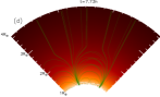
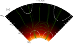
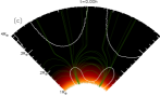
Figure 11: Maps of $Log_{10}(\rho[g/cm^{3}])$ in the $(r-\phi)$ plane passing through the centre of the bipoles at different times for different test simulations. Superimposed are magnetic field lines plotted from the same starting points (green lines) and the contour line of $\beta=1$ (white line). (a) and (d) $T=3$ $MK$, $B_{max}=7$ $G$; (b) and (e) $T=2$ $MK$, $B_{max}=21$ $G$; (c) and (f) $T=1.5$ $MK$, $B_{max}=42$ $G$.

To test the stability, we let the system evolve for a large number of Alfvén times. In the simulation with $B_{max}=7$ $G$, we estimate the Alfvén time $\tau_{Alf}=120$ $s$ as the time it takes an Alfvén wave to travel across a single bipole with a typical speed of $800$ $km/s$. Consequently, the Alfvén time is $\tau_{Alf}=40$ $s$ and $\tau_{Alf}=20s$ for the simulations with $B_{max}=21$ $G$ and $B_{max}=42$ $G$. Fig.11 shows the density contrast (defined in Eq. 10). The plasma density contrast does not show any significant evolution for any of the test simulations, even though small-scale changes occur.

The only test that shows an observable change in the magnetic structure is the one with $T=1.5MK$ and $B_{max}=42$ $G$. This is due to the non-zero values of $p_{bg}$ and $\rho_{bg}$ that lead to a downward bulk motion of plasma in the higher part of the corona, as explained in Sect. 2.2. After this occurs, numerical reconnection takes place, and some of the initially open magnetic field lines reconnect near the outer boundary. However, only a small change in the magnetic configuration can be seen after $\sim 3.3$h, equivalent in this particular simulation to $600$ $\tau_{alf}$ . In the corresponding simulation in Sect. 3.2 where a CME occurs, the magnetic flux rope reaches the top of the domain in less than $0.8$h. Therefore the motions due to the non-zero values of $p_{bg}$ and $\rho_{bg}$ are negligible in comparison to the dynamics produced by the flux rope ejection.

These tests show that the transporting between the GNLFFF and MHD models is possible when including the effects of gravity, a stratified atmosphere, and magnetic field intensity tuning and that these changes do not generate numerical artefacts in the MHD simulation.

References

- Amari et al. (2000) Amari, T., Luciani, J. F., Mikic, Z., & Linker, J. 2000, ApJ, 529, L49
- Antonucci et al. (2004) Antonucci, E., Dodero, M. A., Giordano, S., Krishnakumar, V., & Noci, G. 2004, A&A, 416, 749
- Archontis et al. (2009) Archontis, V., Hood, A. W., Savcheva, A., Golub, L., & Deluca, E. 2009, ApJ, 691, 1276
- Bemporad et al. (2011) Bemporad, A., Mierla, M., & Tripathi, D. 2011, A&A, 531, A147
- Chen & Krall (2003) Chen, J. & Krall, J. 2003, Journal of Geophysical Research (Space Physics), 108, 1410
- Ciaravella et al. (2001) Ciaravella, A., Raymond, J. C., Reale, F., Strachan, L., & Peres, G. 2001, ApJ, 557, 351
- Fan & Gibson (2007) Fan, Y. & Gibson, S. E. 2007, ApJ, 668, 1232
- Forbes & Isenberg (1991) Forbes, T. G. & Isenberg, P. A. 1991, ApJ, 373, 294
- Gary (2001) Gary, G. A. 2001, Sol. Phys., 203, 71
- Gopalswamy (2004) Gopalswamy, N. 2004, in ASSL Vol. 317: The Sun and the Heliosphere as an Integrated System, ed. G. Poletto & S. T. Suess, 201–+
- Gopalswamy et al. (2000) Gopalswamy, N., Lara, A., Lepping, R. P., et al. 2000, Geochim. Res. Lett., 27, 145
- Gopalswamy et al. (2012) Gopalswamy, N., Nitta, N., Akiyama, S., Mäkelä, P., & Yashiro, S. 2012, ApJ, 744, 72
- Guhathakurta et al. (1999) Guhathakurta, M., Fludra, A., Gibson, S. E., Biesecker, D., & Fisher, R. 1999, J. Geophys. Res., 104, 9801
- Hundhausen (1987) Hundhausen, A. J. 1987, in Sixth International Solar Wind Conference, ed. V. J. Pizzo, T. Holzer, & D. G. Sime, 181–+
- Innes et al. (2012) Innes, D. E., Cameron, R. H., Fletcher, L., Inhester, B., & Solanki, S. K. 2012, A&A, 540, L10
- Keppens et al. (2012) Keppens, R., Meliani, Z., van Marle, A. J., et al. 2012, Journal of Computational Physics, 231, 718
- Kliem & Török (2006) Kliem, B. & Török, T. 2006, Physical Review Letters, 96, 255002
- Lee et al. (2009) Lee, J.-Y., Raymond, J. C., Ko, Y.-K., & Kim, K.-S. 2009, ApJ, 692, 1271
- Lin (2004) Lin, J. 2004, Sol. Phys., 219, 169
- Mackay & van Ballegooijen (2006) Mackay, D. H. & van Ballegooijen, A. A. 2006, ApJ, 641, 577
- Manchester et al. (2004) Manchester, W. B., Gombosi, T. I., Roussev, I., et al. 2004, Journal of Geophysical Research (Space Physics), 109, 2107
- Pagano et al. (2013) Pagano, P., Mackay, D. H., & Poedts, S. 2013, A&A, 554, A77
- Pagano et al. (2007) Pagano, P., Reale, F., Orlando, S., & Peres, G. 2007, A&A, 464, 753
- Patsourakos et al. (2010) Patsourakos, S., Vourlidas, A., & Kliem, B. 2010, A&A, 522, A100
- Pomoell & Vainio (2012) Pomoell, J. & Vainio, R. 2012, ApJ, 745, 151
- Powell et al. (1999) Powell, K. G., Roe, P. L., Linde, T. J., Gombosi, T. I., & de Zeeuw, D. L. 1999, Journal of Computational Physics, 154, 284
- Reeves et al. (2010) Reeves, K. K., Linker, J. A., Mikić, Z., & Forbes, T. G. 2010, ApJ, 721, 1547
- Roussev et al. (2012) Roussev, I. I., Galsgaard, K., Downs, C., et al. 2012, Nature Physics, 8, 845
- Temmer et al. (2012) Temmer, M., Vršnak, B., Rollett, T., et al. 2012, ApJ, 749, 57
- Verma et al. (2013) Verma, A. K., Fienga, A., Laskar, J., et al. 2013, A&A, 550, A124
- Vršnak (2001) Vršnak, B. 2001, J. Geophys. Res., 106, 25249
- Zhang et al. (2001) Zhang, J., Dere, K. P., Howard, R. A., Kundu, M. R., & White, S. M. 2001, ApJ, 559, 452
- Zuccarello et al. (2009) Zuccarello, F. P., Jacobs, C., Soenen, A., et al. 2009, A&A, 507, 441