Some exact solutions to the Lighthill–Whitham–Richards–Payne
traffic flow equations II: moderate congestion

Abstract

We find a further class of exact solutions to the Lighthill–Whitham–Richards–Payne (LWRP) traffic flow equations. As before, using two consecutive Lagrangian transformations, a linearization is achieved. Next, depending on the initial density, we either obtain exact formulae for the dependence of the car density and velocity on $x,t$, or else, failing that, the same result in a parametric representation. The calculation always involves two possible factorizations of a consistency condition. Both must be considered. In physical terms, the lineup usually separates into two offshoots at different velocities. Each velocity soon becomes uniform. This outcome in many ways resembles not only Rowlands, Infeld and Skorupski 2013 J. Phys. A: Math. Theor. 46 365202 (part I) but also the two soliton solution to the Korteweg–de Vries equation. This paper can be read independently of part I. This explains unavoidable repetitions. Possible uses of both papers in checking numerical codes are indicated at the end. Since LWRP, numerous more elaborate models, including multiple lanes, traffic jams, tollgates etc. abound in the literature. However, we present an exact solution. These are few and far between, other then found by inverse scattering. The literature for various models, including ours, is given. The methods used here and in part I may be useful in solving other problems, such as shallow water flow.

, ,

1 General history. Formulation of the model

Some nonlinear, partial differential equations of physics, not integrable by inverse scattering or else an inversion of variables, yield their secrets to Lagrangian coordinate methods [1]–[6]. Here we will treat one such equation pair and see a combination of two Lagrangian transformations enable us to solve the one lane moderately congested traffic flow problem explicitly. A further class of solutions is found in parametric form. Calculations augment and reinforce those of part I [7].

In 1955, James Lighthill and Gerald Whitham formulated an equation describing single lane traffic flow, assumed congested enough to justify a fluid model [8]. Richards published in the following year [9]. Next Payne [10] and Whitham [11] added a second equation and replaced the LWR equation with standard continuity. We will call this pair LWRP. Recently the literature on both models has grown considerably, see for example the books by Kern [12] and further references [13]–[22].

Extensions to more than one lane, lane changing, discrete models, higher order effects, as well as numerical work, prevail. One of the original authors has found a Toda lattice like solution to the discrete version of Newell [23], see [24]. In a future paper, we will see if the methods introduced here can be applied to some of these recent extensions of LWRP and LWR.

Other models have been developed [22], and [25]–[36]. However, here we will concentrate on LWRP, remembering that any progress here may have implications for other physical problems, such as gas dynamics.

1.1 The model

Assume a long segment of a one lane road, deprived of entries and exits, only moderately congested by traffic and free of breakdowns admitting a continuous treatment, so as to permit us to postulate the usual equation of continuity:

$$\frac{\partial\rho}{\partial t}+u\frac{\partial\rho}{\partial x}=-\rho\frac{\partial u}{\partial x}.$$ (1)

Here $\rho$ is the density of cars, the maximum of which $\rho_{\mathrm{max}}$ corresponds to a bumper to bumper situation never occurring on our present model, and $u$ is the local velocity. The right hand side of the second, Newtonian equation, formulated by Payne [10] and Whitham [11], is less obvious:

$$\frac{\partial u}{\partial t}+u\frac{\partial u}{\partial x}=\frac{V(\rho)-u}{\tau_{0}}-\frac{\nu_{0}}{\rho}\frac{\partial\rho}{\partial x}.$$ (2)

The first term on the right involves the mean drivers’ reaction time $\tau_{0}$, and the next term models a diffusion effect depending on the drivers’ awareness of conditions beyond the preceding car. The constant $\nu_{0}$ is a parameter that models the effect of gradients on the acceleration. The choice of $V(\rho)$ depends on the quality of the road.

An obvious solution is $\rho$ and $u=V(\rho)$ both constant. Whitham considers this solution in his book and finds that is stable [11].

In part I $V(\rho)$ was a linearly decreasing function of $\rho$:

$$V(\rho)=V_{0}-h_{0}\tau_{0}\sqrt{\nu_{0}}\rho\equiv V_{0}(1-\rho/\rho_{\mathrm{max}}),\qquad\rho\leq\rho_{\mathrm{max}},$$ (3)

where the constant $h_{0}$ is related to $\rho_{\mathrm{max}}$ by

$$h_{0}=\frac{V_{0}}{\rho_{\mathrm{max}}\tau_{0}\sqrt{\nu_{0}}}.$$ (4)

In this paper the analysis will be restricted to $\rho\ll\rho_{\mathrm{max}}$ for which one can approximate $V(\rho)$ by $V_{0}$. In this connection we specify

$$V(\rho)=V_{0}=\mathrm{const},\qquad\rho\leq\rho_{\mathrm{cr}}\ll\rho_{\mathrm{max}}.$$ (5)

This is a form of $V(\rho)$ recently postulated for low density and high quality of the road [33]–[36].

The model used in part I had most common sense properties. The flow of traffic $Q=\rho V(\rho)$ increased from zero for zero density of cars, through a maximum above which traffic becomes congested so that increasing the density no-longer increases the flow, down to an extreme density preventing any motion. The flow against density curve was a continuous parabola. All this is well enough. However, this model can be improved on. When the distances between individual cars are long, increase of density only results in a linear increase in the flow. If you cannot see the cars preceding and following you, a possible small increase in the car density will hardly be noticed. Thus the flow is a linear function of the density. Thus the left hand portion of $V(\rho)$ should be a constant up to some $\rho_{\mathrm{cr}}$ and the flow is $\rho V_{0}$. Calculations simplify as long as we stay away from $\rho_{\mathrm{cr}}$. The value of $\rho_{\mathrm{cr}}$ will depend on the quality of the road.

We introduce dimensionless variables by replacing

$$t\ \to\ t\,\tau_{0},\qquad(u,V_{0})\to\ (u,V_{0})\,\sqrt{\nu_{0}},\qquad x\ \to\ x\,\sqrt{\nu_{0}}\tau_{0},\qquad\rho\to\ \rho\,(h_{0}\tau_{0})^{-1}.$$ (6)

This leaves the continuity equation unchanged, and the Newtonian equation takes the form:

$$\frac{\partial u}{\partial t}+u\frac{\partial u}{\partial x}=V_{0}-u-\frac{1}{\rho}\frac{\partial\rho}{\partial x},$$ (7)

slightly simpler than in part I. Here in part II we treat situations that never become very congested ($\rho\ll\rho_{\mathrm{max}}$) which for the dimensionless quantities requires that

$$\rho\leq\rho_{\mathrm{cr}}\ll V_{0}.$$ (8)

Our model is a macroscopic one in which the traffic is treated as a fluid flow. This is in contrast to the microscopic models involving motions of individual cars and hybrid models combining elements of both.

2 Introducing Lagrangian coordinates

(The Reader who has read part I can proceed to section 3.)

The non-linearity on the left hand side of equations (1) and (7) can be eliminated by introducing Lagrangian coordinates: $\xi(x,t)$, the initial position (at $t=0$) of a fluid element which at time $t$ was at $x$, and time $t$. In this description, the independent variable $x$ becomes a function of $\xi$ and $t$, as are the fluid parameters $\rho(\xi,t)=\rho(x(\xi,t),t)$ and $u(\xi,t)=u(x(\xi,t),t)$.

Here and in what follows we adopt the convention that a superposition of two functions which introduces a new variable is denoted by the same symbol as the original function, but of the new variable. Denoting by $f$ either $\rho$ or $u$, the basic transformation between Eulerian coordinates $x,t$ and Lagrangian ones $\xi,t$ can be written as

$$x(\xi,t)=\xi+\int_{0}^{t}u(\xi,t^{\prime})\,\mathrm{d}t^{\prime},\qquad\frac{\partial x}{\partial t}=u(\xi,t),\qquad\frac{\partial f(\xi,t)}{\partial t}=\frac{\partial f(x,t)}{\partial t}+u\frac{\partial f(x,t)}{\partial x}.$$ (9)

We denote by $s(\xi)$ the number of cars between the last one at $\xi=\xi_{\mathrm{min}}$ and that at $\xi$:

$$s(\xi)=\int_{\xi_{\mathrm{min}}}^{\xi}\rho_{0}(\xi^{\prime})\,\mathrm{d}\xi^{\prime},\qquad\rho_{0}(\xi)=\rho(x=\xi,t=0)$$ (10)

where $\rho_{0}(\xi)$ is the initial mass density distribution.

Here and in what follows, the subscript $0$ always refers to $t=0$. We will also use the superscript $0$ to refer to $\xi=0$.

Here $\rho_{0}(\xi)$ is positive. Hence $s(\xi)$ is an increasing function starting at $s(\xi_{\mathrm{min}})=0$, and one can introduce a uniquely defined inverse function $\xi(s)$. The initial position of a fluid element can be specified by either $\xi$ or $s$.

If a small initial interval $\mathrm{d}\xi$ at $t=0$ becomes $\mathrm{d}x$ at time $t$, mass conservation requires:

$$\mathrm{d}s=\rho_{0}(\xi)\mathrm{d}\xi=\rho(x,t)\mathrm{d}x.$$ (11)

This leads to a mass conservation equation in Lagrangian variables:

$$\frac{\partial x(s,t)}{\partial s}=\frac{1}{\rho(s,t)},$$ (12)

and to a useful operator identity

$$\frac{1}{\rho(x,t)}\frac{\partial}{\partial x}=\frac{1}{\rho_{0}(\xi)}\frac{\partial}{\partial\xi}=\frac{\partial}{\partial s}.$$ (13)

Integrating (12) over $s^{\prime}$ from $s(\xi=0)$ to $s$, we obtain the continuity equation in integral form:

$$X(s,t)\equiv x(s,t)-x(s^{0},t)=\int_{s^{0}}^{s}\frac{\mathrm{d}s^{\prime}}{\rho(s^{\prime},t)},\qquad s^{0}=s(\xi=0).$$ (14)

This indicates that if we know the car density in Lagrangian coordinates $\rho(s,t)$, we can determine the evolving shape of the line of traffic, where the distance $X$ is measured from the $\xi=0$ car.

The analogue of the continuity equation (1) is obtained by differentiating (12) by $t$. Using the middle part of (9) we obtain

$$\frac{\partial\psi(s,t)}{\partial t}=\frac{\partial u}{\partial s},\qquad\psi=\frac{1}{\rho}.$$ (15)

The Newtonian equation in Lagrangian coordinates is obtained from (7) and (13):

$$\frac{\partial u(s,t)}{\partial t}+u=V_{0}-\frac{\partial\rho}{\partial s}.$$ (16)

Equation (16) can be solved to express $u(s,t)$ in terms of $\rho$. Again, using the middle part of (9) we can also calculate $x(s,t)$:

$$u(s,t) =\mathrm{e}^{-t}\biggl{[}\int_{0}^{t}N(s,t^{\prime})\mathrm{e}^{t^{\prime}}\,\mathrm{d}t^{\prime}+u(s,0)\biggr{]},$$ (17)

$$N(s,t) =V_{0}-\frac{\partial\rho}{\partial s},$$ (18)

$$x(s,t) =\xi(s)+\int_{0}^{t}u(s,t^{\prime})\,\mathrm{d}t^{\prime}$$ (19)

$$=\xi(s)+u(s,0)-u(s,t)+\int_{0}^{t}N(s,t^{\prime})\,\mathrm{d}t^{\prime},$$

where the function $u(s,0)$ will be determined later.

3 Finding the fluid density

Differentiating the Newtonian equation (16) by $s$, and using continuity (15), we obtain one equation for $\psi$:

$$\frac{\partial^{2}\psi}{\partial t^{2}}-\frac{\partial}{\partial s}\Bigl{(}\frac{1}{\psi^{2}}\frac{\partial\psi}{\partial s}\Bigr{)}+\frac{\partial\psi}{\partial t}=0.$$ (20)

In part I, there was an extra $\partial(1/\psi)/\partial s$ term, causing the equation to have a symmetry when $\psi\to 1/\psi$, $s\to t$. Every solution had a formal twin. This symmetry is now lost, even though equation (20) is simpler.

Equation (20) can be factorized in two possible ways, I and II:

$$\mathrm{I:\ }\qquad\Bigl{(}\frac{\partial}{\partial t}+\frac{\partial}{\partial s}\frac{1}{\psi}\Bigr{)}\Bigl{(}\frac{\partial\psi}{\partial t}-\frac{1}{\psi}\frac{\partial\psi}{\partial s}+\psi\Bigr{)}=0,$$ (21)

and

$$\mathrm{II:}\qquad\Bigl{(}\frac{\partial}{\partial t}-\frac{\partial}{\partial s}\frac{1}{\psi}\Bigr{)}\Bigl{(}\frac{\partial\psi}{\partial t}+\frac{1}{\psi}\frac{\partial\psi}{\partial s}+\psi\Bigr{)}=0.$$ (22)

We will find that the second factor in (21) best yields solutions such that $X\geq 0$, whereas that in (22) rules $X<0$, where $X$ is always the distance from the car that started at $x=0$. In both (21) and (22), one term in the second factor is absent as compared to part I.

In what follows, we will find solutions for which the second factor in one of equations (21), (22) vanishes. We follow motion from left to right. Factorization also means that we can only introduce the initial value of the density (or $\psi$). The initial velocity $u(s,t=0)$ will then follow except for a universal constant. We will have more to say about this later on.

The nonlinearities in (21) and (22) (second factors) can be eliminated if one transforms the variables $s,t$ to $\eta,t$ in a way similar to the Lagrangian transformation (9):

$$s(\eta,t)=\eta\mp\int_{0}^{t}\frac{\mathrm{d}t^{\prime}}{\psi(\eta,t^{\prime})},\qquad\frac{\partial s}{\partial t}=\mp\frac{1}{\psi(\eta,t)},\qquad\frac{\partial\psi(\eta,t)}{\partial t}=\frac{\partial\psi(s,t)}{\partial t}\mp\frac{1}{\psi}\frac{\partial\psi}{\partial s}\,.$$ (23)

Solving the resulting linear equation

$$\frac{\partial\psi(\eta,t)}{\partial t}=-\psi$$

we obtain, in view of the fact that s and $\eta$ are identical at $t=0$,

$$\psi(\eta,t)=\mathrm{e}^{-t}\psi_{0}(\eta),\qquad\psi_{0}(\eta)\equiv\psi(s=\eta,0).$$ (24)

For this $\psi(\eta,t)$ we have

$$\int_{0}^{t}\frac{\mathrm{d}t^{\prime}}{\psi}=\frac{\mathrm{e}^{t}-1}{\psi_{0}(\eta)},$$ (25)

and finally, back to $\rho=1/\psi$ and using (23),

$$s=\eta\mp\rho_{0}(\eta)A(t),\qquad\rho_{0}(\eta)=\rho_{0}(s=\eta),\qquad A(t)=\mathrm{e}^{t}-1.$$ (26)

In this relation, defining $s$ in terms of $\eta$ and $t$, $\rho_{0}(\eta)$ is defined by (10) but is expressed in terms of $s$, where one has to rename $s$ to $\eta$. The same procedure applies to $\psi_{0}(\eta)$ given by (24).

Using (24), we can express $\rho$ in terms of $\eta$ and $t$:

$$\rho(\eta,t)=\mathrm{e}^{t}\rho_{0}(\eta),$$ (27)

which tends to $\rho_{0}(s)$ as $t\to 0$.

We are now in a position to determine the function $u(s,0)$ needed in equations (17) and (19). Differentiate (16) by $s$ and then subtract both sides of (20) from the result to obtain

$$\Bigl{(}\frac{\partial}{\partial t}+1\Bigr{)}\Bigl{(}\frac{\partial\psi}{\partial t}-\frac{\partial u}{\partial s}\Bigr{)}=0.$$ (28)

Solved by

$$\frac{\partial\psi}{\partial t}-\frac{\partial u}{\partial s}=f(s)e^{-t}.$$ (29)

Therefore, if $f(s)=0$, equation (15) will be valid for all time. All we require is

$$\Bigl{[}\frac{\partial\psi}{\partial t}-\frac{\partial u}{\partial s}\Bigr{]}_{t=0}=0,\qquad\mathrm{i.e.}\qquad\frac{\partial u(s,0)}{\partial s}=\frac{\partial\psi_{0}}{\partial t}.$$ (30)

This result, along with either (21) or (22), leads to

$$\frac{\partial u(s,0)}{\partial s}=\pm\frac{1}{\psi_{0}}\frac{\partial\psi_{0}}{\partial s}-\psi_{0}.$$

Integrating over $s^{\prime}$ from $s^{0}\ (=s(\xi=0))$ to $s$ and transforming the result to $\xi$, we end up with

$$u(\xi,0)=u_{0}-\xi\mp\ln\frac{\rho_{0}(\xi)}{a},\qquad a=\rho_{0}(\xi=0),$$ (31)

where $u_{0}=u(\xi=0,0)\geq 0$ is arbitrary.

The last task is to determine $u(s,t)$, $x(s,t)$, and $X(s,t)$, given by (17), (19), and (14), in terms of $\eta$. Using (27), (26) and (18) we find the integrand $N$:

$$N(s,t) =V_{0}-\frac{\partial\rho}{\partial s}=V_{0}-\frac{\partial\rho/\partial\eta}{\partial s/\partial\eta}$$ (32)

$$=V_{0}\pm 1-\frac{\pm 1+\rho_{0}^{\prime}(\eta)}{1\mp\rho_{0}^{\prime}(\eta)(\mathrm{e}^{t}-1)},$$

which tends to $V_{0}\pm 1$ as $t\to\infty$. Here $\eta=\eta(s,t)$ must be found as a solution of equation (26) which is often transcendental. If that is the case, the integrals (17) and (19) must be calculated numerically. On the other hand, the integral in (14) can be calculated analytically:

$$X(s,t) \equiv x(s,t)-x(s^{0},t)=\int_{\eta^{0}}^{\eta}\frac{\partial s^{\prime}/\partial\eta^{\prime}}{\rho(\eta^{\prime},t)}\,\mathrm{d}\eta^{\prime}$$ (33)

$$=\mathrm{e}^{-t}\biggl{[}\xi(s=\eta)-\xi(s=\eta^{0})\mp A(t)\ln\frac{\rho_{0}(\eta)}{\rho_{0}(\eta^{0})}\biggr{]},$$

where $\eta=\eta(s,t)$ and $\eta^{0}=\eta(s^{0},t)$ are defined implicitly by (26).

Restrictions on $\rho_{0}(\xi)$ are given in part I.

4 Two exponential profiles of the initial fluid density

We will see that two exponential profiles of the initial fluid density

$$\rho_{0}(\xi)=a\exp(-\lambda\xi),\qquad \xi\geq 0,\qquad\mathrm{i.e.}\qquad\xi_{\mathrm{min}}=0,$$ (34)

$$\rho_{0}(\xi)=a\exp(\lambda\xi),\qquad \xi\leq 0,\qquad\mathrm{i.e.}\qquad\xi_{\mathrm{min}}=-\infty,$$ (35)

play a special role here, as in their case it is possible to eliminate the auxiliary variable $\eta$, and even find the fluid density $\rho$ in terms of $X$ and $t$.

Using equation (10) we first find

$$s^{0}=s(\xi=0)=\int_{\xi_{\mathrm{min}}}^{0}\rho_{0}(\xi^{\prime})\,\mathrm{d}\xi^{\prime}=\cases{0&for (\ref{ic}),\\ \frac{a}{\lambda}&for (\ref{ic2}),}$$ (36)

and then calculate

$$s(\xi) =s^{0}+\int_{0}^{\xi}\rho_{0}(\xi^{\prime})\,\mathrm{d}\xi^{\prime}=s^{0}\mp\frac{a}{\lambda}\Bigl{(}\exp(\mp\lambda\xi)-1\Bigr{)}$$ (37)

$$=\cases{\frac{a}{\lambda}\Bigl{(}1-\exp(-\lambda\xi)\Bigr{)}&for (\ref{ic}),\\ \frac{a}{\lambda}\exp(\lambda\xi)&for (\ref{ic2}).}$$

The inverse functions are given by

$$\xi(s)=\mp\frac{1}{\lambda}\ln\Bigl{(}1\mp{\textstyle\frac{\lambda}{a}}(s-s^{0})\Bigr{)}=\cases{-\frac{1}{\lambda}\ln\Bigl{(}1-{\textstyle\frac{\lambda s}{a}}\Bigr{)}&for (\ref{ic}),\\ \frac{1}{\lambda}\ln\frac{\lambda s}{a}&for (\ref{ic2}).}$$ (38)

Using this formula we can transform the initial conditions (34) and (35) given above in $x,t$ to $s,t$:

$$\rho_{0}(s)=a\mp\lambda(s-s^{0})=\cases{a-\lambda s&for (\ref{ic}),\\ \lambda s&for (\ref{ic2}).}$$ (39)

We now look for solutions to equations (21) and (22) that recreate the above initial conditions as $t$ tends to zero.

Replacing $s$ by $\eta$ in (39) and using the $\rho_{0}(\eta)$ so obtained in (26) and (27), we obtain

$$s=\eta+A(t)\,\Bigl{[}\lambda(\eta-s^{0})\mp a\Bigr{]},\qquad A(t)=\mathrm{e}^{t}-1,$$ (40)

leading to

$$\eta(s,t)=\frac{s+A(t)(\lambda s^{0}\pm a)}{1+\lambda A(t)},$$ (41)

and

$$\rho(s,t)=\frac{\mathrm{e}^{t}\rho_{0}(s)}{1+\lambda A(t)}\equiv\frac{\rho_{0}(s)}{\lambda+(1-\lambda)\mathrm{e}^{-t}},$$ (42)

where $\rho_{0}(s)$ is given by (39). In the limit $t\to 0$, we obtain $\rho(s,t)\to\rho_{0}(s)$.

Using (42) and (31) we can determine $N(\xi,t)$ and $u(\xi,0)$ needed in equations (17)–(19):

$$N(\xi,t) =V_{0}\pm 1\pm\frac{\lambda-1}{1+\lambda A(t)}$$ (43)

$$\to V_{0}\pm 1\qquad\mathrm{as}\ t\to\infty,$$

$$u(\xi,0) =u_{0}+(\lambda-1)\xi.$$ (44)

Calculating the integrals in (17) and (19), we find the fluid velocity $u(\xi,t)$ and characteristics $x(\xi,t)$ parametrized by the initial fluid element position $\xi$:

$$u(\xi,t) =V_{0}\pm 1+\mathrm{e}^{-t}$$ (45)

$$\quad\times\biggl{[}u_{0}+(\lambda-1)\xi-V_{0}\mp 1\pm\frac{\lambda-1}{\lambda}\ln\Bigl{(}\lambda\mathrm{e}^{t}+1-\lambda\Bigr{)}\Bigr{]}$$

$$\to V_{0}\pm 1\qquad\mathrm{as}\ t\to\infty,$$

$$x(\xi,t) =\xi+(V_{0}\pm 1)t+(1-\mathrm{e}^{-t})[u_{0}+(\lambda-1)\xi-V_{0}\mp 1]$$ (46)

$$\quad\mp\frac{\lambda-1}{\lambda}\biggl{\{}\biggl{[}\mathrm{e}^{-t}+\frac{\lambda}{1-\lambda}\biggr{]}\ln[(1-\lambda)\mathrm{e}^{-t}+\lambda]+t\mathrm{e}^{-t}\biggr{\}}.$$

We will now express $\rho$ directly in terms of $X$ by using (14), (39) and (42). The result is

$$\rho(X,t)=\frac{a}{\lambda+(1-\lambda)\mathrm{e}^{-t}}\exp\biggl{(}\mp\frac{\lambda}{\lambda+(1-\lambda)\mathrm{e}^{-t}}X\biggr{)}.$$ (47)

The shapes evolve from $a\exp(\mp\lambda X)$ profiles to $(a/\lambda)\exp(\mp X)$ profiles as $t$ goes from $0$ to $\infty$. The relevant drawings, shown in figures 1 to 3, are very similar to figures 1 to 4 of part I. Total mass is conserved and is $a/\lambda$ in each segment. This is now easily seen at all times (in part I for $t\to\infty$ only).

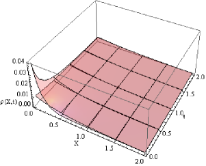
Figure 1: Two density profiles for various times as found from our solution (I). Here $a=0.01$, $\lambda=2$ in the first case, and $a=0.04$, $\lambda=8$ in the second one. Nevertheless, the emerging profiles are seen to be identical after a while. The value of $a$ for each surface can be seen as equal to $\rho(0,0)$.

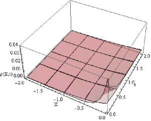
Figure 2: Two density profiles for various times as found from our solution (II). Here $a=0.01$, $\lambda=2$ in the first case, and $a=0.04$, $\lambda=8$ in the second one. Nevertheless, the emerging profiles are seen to be identical after a while. The value of $a$ for each surface can be seen as equal to $\rho(0,0)$.

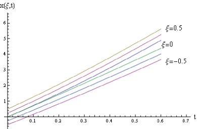
Figure 3: Characteristics $x(\xi,t)$ as functions of $t$ for $\xi=0,\>0.25,\>05,$ and $\xi=0,\>-0.25,\>-05$, $a=0.01$, $\lambda=2$, $u_{0}=7$, and $V_{0}=10$.

5 Initial density profiles that can be treated parametrically

In this section we present a few initial density profiles satisfying the applicability conditions of our theory as formulated in part I, see figure 4.

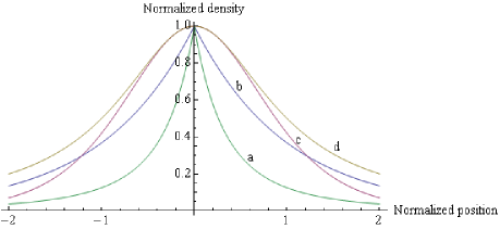
Figure 4: Normalized density profiles $\bar{\rho}_{0}=\rho_{0}/a$ versus normalized position $\bar{\xi}=\lambda\xi$ for $\rho_{0}(\xi)$ given by (a): (34) and (35), (b): (50) for $b=1$, $r=3$, (c): (48), and (d): (49).

Detailed calculations will be performed for a pair of cases:

$$\rho_{0}(\xi)=\frac{a}{\cosh^{2}(\lambda\xi)}\equiv a\,\bigl{[}1-\tanh^{2}(\lambda\xi)\bigr{]},$$ (48)

where either $0\leq\xi<\infty$ in case I, or $-\infty<\xi\leq 0$ in case II.

The fact that the derivative $\mathrm{d}\rho_{0}(\xi)/\mathrm{d}\xi$ vanishes at $\xi=0$, in contrast to the exponential profiles (34) and (35), will influence the time evolution in case I, see figure 5.

The remaining profiles will have a power law behaviour at infinity, $\rho_{0}(\xi)\to(\pm\xi)^{-r}$ as $\pm\xi\to\infty$, where $r$ is a real number greater than unity for integrability:

$$\rho_{0}(\xi)=\frac{a}{1+(\lambda\xi)^{2}},$$ (49)

and

$$\rho_{0}(\xi)=a\,\frac{b^{r}}{(\pm\lambda\xi+b)^{r}},\qquad b>0,\qquad r>1,$$ (50)

where the upper sign refers to case I, $\xi\geq 0$, and the lower one to case II, $\xi\leq 0$.

By analogy to the exponential profiles (34) and (35), each pair of symmetric cases can be treated in a single calculation. For $\rho_{0}(\xi)$ given by (48) we first find

$$s^{0}=s(\xi=0)=\int_{\xi_{\mathrm{min}}}^{0}\rho_{0}(\xi^{\prime})\,\mathrm{d}\xi^{\prime}=\cases{0&for $\xi\geq 0$,\\ \frac{a}{\lambda}&for $\xi\leq 0$,}$$ (51)

and then calculate

$$s(\xi)=s^{0}+\int_{0}^{\xi}\rho_{0}(\xi^{\prime})\,\mathrm{d}\xi^{\prime}=s^{0}+\frac{a}{\lambda}\tanh(\lambda\xi).$$ (52)

The inverse functions are given by

$$\xi(s)=\frac{1}{2\lambda}\ln\frac{1+\lambda(s-s^{0})/a}{1-\lambda(s-s^{0})/a}=\cases{\frac{1}{2\lambda}\ln\frac{1+\lambda s/a}{1-\lambda s/a}&for $\xi\geq 0$,\\ \frac{1}{2\lambda}\ln\frac{\lambda s/a}{2-\lambda s/a}&for $\xi\leq 0$.}$$ (53)

Using $\tanh(\lambda\xi)$ calculated from (52) in (48) we obtain

$$\rho_{0}(s)=a\Bigl{[}1-\Bigl{(}\lambda(s-s^{0})/a\Bigr{)}^{2}\Bigr{]}=\cases{a[1-(\lambda s/a)^{2}]&for $\xi\geq 0$,\\ \lambda s(2-\lambda s/a)&for $\xi\leq 0$.}$$ (54)

Replacing here $s$ by $\eta$ and using the $\rho_{0}(\eta)$ so obtained in (26) and (32) along with (52) we find equations defining $\eta(\xi,t)$ and the integrand $N(\eta,t)$ needed in equations (17)–(19):

$$\frac{a}{\lambda}\tanh(\lambda\xi)=\eta-a[1-(\lambda\eta/a)^{2}]A(t),\qquad \mathrm{for}\ \xi\geq 0,$$ (55)

$$\frac{a}{\lambda}\bigl{[}1+\tanh(\lambda\xi)\bigr{]}=\eta+\lambda\,\eta(2-\lambda\eta/a)A(t),\qquad \mathrm{for}\ \xi\leq 0,$$ (56)

$$N(\eta,t)=V_{0}\pm 1+\frac{\mp 1-f(\eta)}{1\mp f(\eta)A(t)},$$ (57)

where

$$f(\eta)=\cases{-2\eta\lambda^{2}/a+a&for $\xi\geq 0$,\\ 2\lambda\Bigl{[}\eta(1-\lambda/a)+1\Bigr{]}&for $\xi\leq 0$.}$$ (58)

In a similar way we can determine $X(\eta,t)$ by using (33) along with (53) and (54) with $s=\eta$:

$$X=-\frac{\mathrm{e}^{-t}}{\lambda}\biggl{[}\Bigl{(}\lambda A(t)+\frac{1}{2}\Bigr{)}\ln\frac{1-\lambda\eta/a}{1-\lambda\eta^{0}/a}+\Bigl{(}\lambda A(t)-\frac{1}{2}\Bigr{)}\ln\frac{1+\lambda\eta/a}{1+\lambda\eta^{0}/a}\biggr{]}\qquad \mathrm{for}\ \xi\geq 0,$$ (59)

$$X=\frac{\mathrm{e}^{-t}}{\lambda}\biggl{[}\Bigl{(}\lambda A(t)+\frac{1}{2}\Bigr{)}\ln\frac{\eta}{\eta^{0}}+\Bigl{(}\lambda A(t)-\frac{1}{2}\Bigr{)}\ln\frac{2-\lambda\eta/a}{2-\lambda\eta^{0}/a}\biggr{]} \mathrm{for}\ \xi\leq 0.$$ (60)

Surprisingly similar to the corresponding equation in part I. Again, just one term has dropped out.

Using $X(\eta,t)$ given by these formulae and $\rho(\eta,t)$ given by (27), where $\eta(\xi,t)$ is defined implicitly by either (55) or (56), we obtain $\rho(X,t)$ in parametric form: $\rho(\xi,t)$ and $X(\xi,t)$. This form is appropriate for the ParametricPlot3D command of Mathematica. The results are shown in figures 5 and 6. They resemble those shown in figures 6 and 7 of part I.

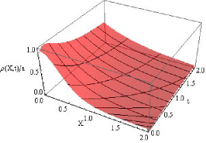
Figure 5: The normalized fluid density $\rho(X,t)/a$ represented parametrically as found from our solution (I). Here $a=0.01$, $\lambda=2$. The mesh lines correspond to $t=\mathrm{const}$ or $\xi=0,\>0.25,\>0.5,\>0.75,\dots$. Each value of $\xi$ is equal to $X$ at $t=0$.

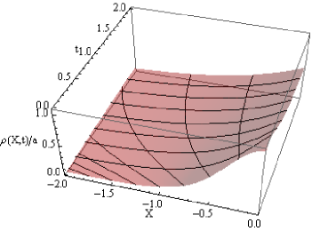
Figure 6: The normalized fluid density $\rho(X,t)/a$ as in figure 5 but as found from our solution (II). Here again $a=0.01$, $\lambda=2$, and $\xi=0,\>-0.25,\>-0.5,\>-0.75,\dots$, see $X$ at $t=0$.

The characteristics $x(\xi,t)$ can be found from equations (17)–(19) by numerical integration, where the integrand $N(\xi,t)$ is defined by (57) and either (55) or (56), and

$$u(\xi,0)=u_{0}-\xi\mp\Bigl{\{}\frac{a}{\lambda}\tanh(\lambda\xi)-2\,\ln\Bigl{[}\cosh(\lambda\xi)\Bigr{]}\Bigr{\}},$$ (61)

see equations (31), (48) and (52). The results, depending on two parameters $V_{0}$ and $u_{0}$, are shown in figure 7.

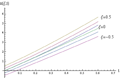
Figure 7: Characteristics $x(\xi,t)$ as functions of $t$ for $\xi=0,\>0.25,\>05,$ and $\xi=0,\>-0.25,\>-05$, $a=0.01$, $\lambda=2$, $u_{0}=7$, and $V_{0}=10$.

A characteristic feature of the plots representing the density given in parametric form, $\rho(\xi,t)$ and $X(\xi,t)$, is that the mesh lines correspond to $\xi=\mathrm{const}$, and $t=\mathrm{const}$, see figures 5 and 6. For the density given explicitly, $\rho(X,t)$, they correspond to $X=\mathrm{const}$, and $t=\mathrm{const}$. Each point on a $\xi=\mathrm{const}$ mesh line gives us both the actual position $X$ and the associated density at time $t$, for the car that started from $X=\xi$ at $t=0$. This information is given in the frame moving with the discontinuity at $\xi=0$. The motion of these frames in turn is described by the characteristics labeled $\xi=0$ in figure 7.

Adding cases I and II, we have a solution such that the initial configuration splits in the middle, resulting once again in a slower cavalcade following a faster one, see figure 7. This is rather like a two soliton solution of the Korteweg–de Vries equation, see e.g. [2].

6 Summary

The LWRP model for traffic flow leaves the flow dependence on density open. This dependence must be found for a specific road. Common sense implies some ramifications. When there are no cars, flow is gone, so the $Q(\rho)$ curve emerges from zero. A car a mile means no interaction, so $Q=V(\rho=0)\rho$ for a while. As $\rho$ increases, interaction slows the growth of $Q(\rho)$ down until a critical density is achieved. Now increase in density is balanced by the interaction and $\mathrm{d}Q/\mathrm{d}\rho=0$. Next $Q$ decreases down to zero at a complete traffic jam density. Details vary from road to road, not to mention the make of the cars. However, diagrams will have the following division in common:

1. $\rho\leq\rho_{\mathrm{cr}}$, straight line indicating growth of $Q(\rho)$

2. $Q(\rho)$ still grows, but at a decreasing pace, until a maximum is reached

3. $Q(\rho)$ decreases with increasing $\rho$ down to zero at jam density.

Here in part II we concentrated on the first region, whereas in part I the whole curve was approximated by a parabola. Differences were seen not be too important, especially for small $a\ (=\rho_{0}(t=0))$.

Our solutions both confirm and augment those of part I. They are somewhat similar but simpler. Our exact solutions once again converge to single or double stationary travelling wave structures after a few $\tau_{0}$, see figures 1 and 2.

It should be stressed that a complete solution is only possible if we combine our two factorized equations, I and II.

The solutions presented here and in part I can be used to check numerical codes before using them on more complicated situations. Simpler ones than here in part II would be hard to find!

References

References

- [1] Infeld E and Rowlands G 1989 Relativistic bursts Phys. Rev. Lett.62 1122–5 Infeld E and Rowlands G 1997 Lagrangian picture of plasma physics I J. Tech. Phys. 38 607–45 Infeld E and Rowlands G 1998 Lagrangian picture of plasma physics II J. Tech. Phys. 39 3–35
- [2] Infeld E and Rowlands G 2000 Nonlinear Waves, Solitons and Chaos 2nd edn (Cambridge: Cambridge University Press)
- [3] Infeld E, Rowlands G and Skorupski A A 2009 Analytically solvable model of nonlinear oscillations in a cold but viscous and resistive plasma Phys. Rev. Lett.102 145005
- [4] Skorupski A A and Infeld E 2010 Nonlinear electron oscillations in a viscous and resistive plasma Phys. Rev. E 81 056406
- [5] Armstrong T and Montgomery D 1967 Asymptotic state of the two-stream instability J. Plasma Phys. 1 425–33
- [6] Jordan P M and Puri P 2002 Exact solution for the unsteady plane Couette flow of a dipolar fluid Proc. R. Soc.A 458 1245–72
- [7] Rowlands G, Infeld E and Skorupski A A 2013 Some exact solutions to the Lighthill–Whitham–Richards–Payne traffic flow equations J. Phys. A: Math. Gen.46 365202
- [8] Lighthill M J and Whitham G B 1955 On kinematic waves: I. Fluid movement in long rivers Proc. R. Soc.A 229 281–316 Lighthill M J and Whitham G B 1955 On kinematic waves: II. Theory of traffic flow on long crowded roads Proc. R. Soc.A 229 317–45
- [9] Richards P I 1956 Shock waves on the highway Oper. Res. 4 42–51
- [10] Payne H J 1971 Models of freeway traffic and control Mathematical Models of Public Systems (Simulation Councils Proceedings vol 1, La Jolla California: Simulation Council) 51–60
- [11] Whitham G B 1974 Linear and Nonlinear Waves (New York: Wiley) chap 3
- [12] Kern B S 2003 The Physics of Traffic Flow (Berlin: Springer) Kern B S 2009 Introduction to Modern Traffic Flow, Theory and Control (Berlin: Springer)
- [13] Chandler R E, Herman R and Montroll E W 1958 Traffic dynamics: studies in car following Oper. Res. 6 165–84
- [14] Greenberg H 1959 An analysis of traffic flow Oper. Res. 7 79–85
- [15] Herman R, Montroll E W, Potts R B and Rothery R W 1959 Traffic dynamics: analysis of stability in car following Oper. Res. 7 86–106
- [16] Jin W L and Zhang H M 2003 The formation and structure of vehicle clusters in the Payne–Whitham traffic flow model Transp. Res. 37 207–23
- [17] Kerner B S, Klenov L and Konhauser P 1997 Asymptotic theory of traffic flow Phys. Rev. E 56 4200–16
- [18] Komentani E and Sasaki T 1958 On the stability of traffic flow Oper. Res. Japan 2 11–26
- [19] Lua Y et al2008 Explicit construction of solutions for the Lighthill–Whitham–Richards traffic flow model with a piecewise traffic flow density model Transp. Res. 42 355–72
- [20] Papageorgiou M 1983 Application of Automatic Control Concepts in Traffic Flow and Control (Berlin: Springer)
- [21] Zhang M, Shu C, Wong G C K and Wong S C 2003 A weighted essentially non-oscillatory numerical scheme for a multi-class LWR traffic flow model J. Comput. Phys. 191 639–59
- [22] Treiber, M and Kesting, A 2013 Traffic Flow Dynamics (Berlin: Springer)
- [23] Newell G F 1961 Nonlinear effects in the dynamics of car following Oper. Res. 9 209–29
- [24] Whitham G B 1990 Exact solutions for a discrete system arising in traffic flow Proc. R. Soc.A 428 49–69
- [25] Rascle M 2002 An improved macroscopic model of traffic flow Math. Comput. Modelling 35 581–90
- [26] Ge H X, Zhu H B and Dai S Q 2006 Effect of looking backwards in a cooperative driving car flowing model Eur. Phys. J. B 54 503–7
- [27] Rascle M, Degond P and Delitala M 2008 Formation and evolution of traffic jams Arch. Ration. Mech. Anal. 187 185–220
- [28] Gaididei Yu B et al2009 Analytical solutions of jam pattern formation on a ring for a class of optimal traffic models New J. Phys. 11 073012
- [29] Vikram D, Mittal S and Chakraborty D 2011 A stabilized finite element formulation for continuum models of traffic flow Comput. Modelling Eng. Sci. 79 237–60
- [30] Aw A and Rascle M 2000 Resurrection of “second order” models of traffic flow SIAM J. App. Math. 60 916–938
- [31] Bellomo N and Dogbé C 2011 On the modelling of traffic and crowds: a survey of models, speculations, and perspectives SIAM Review 53 409–63
- [32] Helbing D and Treiber M 2008 Derivation of a fundamental diagram for urban traffic flow Eur. Phys. J. B 70 223–41
- [33] Belloquid A, De Angelis E and Fermo L 2012 Towards a modelling of vehicular traffic as a complex system Math. Models, Meth. App. Sci., Supplement 1, 22 114006
- [34] Fermo L and Tosin A 2013 A fully-discrete-state kinetic theory approach to modeling vehicular traffic SIAM J. App. Math. 73 1533–56
- [35] Degond P and Delitala M 2008 Modelling and simulation of vehicular traffic jam formation Kinetic and Related Models 1 278–93
- [36] Dolfin M 2014 Boundary conditions for first order macroscopic model of vehicular traffic flow in the presence of tollgates App. Math. Comput. 234 260–8