Abstract

Solving semidefinite programs (SDP) in a short time is the key to managing various mathematical optimization problems. The matrix-completion primal-dual interior-point method (MC-PDIPM) extracts a sparse structure of input SDP by factorizing the variable matrices. In this paper, we propose a new factorization based on the inverse of the variable matrix to enhance the performance of MC-PDIPM. We also use multithreaded parallel computing to deal with the major bottlenecks in MC-PDIPM. Numerical results show that the new factorization and multithreaded computing reduce the computation time for SDPs that have structural sparsity.

Keywords
Semidefinite programs, Interior-point methods, Matrix completion, Multithreaded computing

AMS Classification
90 Operations research, mathematical programming, 90C22 Semidefinite programming, 90C51 Interior-point methods, 97N80 Mathematical software, computer programs.

1 Introduction

Semidefinite programs (SDP) have become one of main topics of mathematical optimization, because of its wide range application from combinatorial optimization [9] to quantum chemistry [7, 21] and sensor network localization [4]. A survey of its many applications can be found in Todd’s paper [24], and the range is still expanding. Moreover, there is no doubt that solving SDPs in a short time is the key to managing such applications. The primal-dual interior-point method (PDIPM) [1, 11, 15, 18, 22] is often employed since it can solve SDPs in a polynomial time, and many solvers are based on it, for example, SDPA [26], CSDP [5], SeDuMi [23], and SDPT3 [25]. A recent paper [27] reports that integration with parallel computing enables one to solve large-scale SDPs arising in practical applications.

A major difficulty with PDIPM is that the primal variable matrix $X$ must be handled as a fully dense matrix even when all the input data matrices $\mbox{\boldmath$A$}_{0},\ldots,\mbox{\boldmath$A$}_{m}$ are considerably sparse. The standard form in this paper is the primal-dual pair;

$$(\mbox{$\cal P$}) \begin{array}[]{lcl}\min&:&\mbox{\boldmath$A$}_{0}\bullet\mbox{\boldmath$X$}\\ \mbox{subject to}&:&\mbox{\boldmath$A$}_{k}\bullet\mbox{\boldmath$X$}=b_{k}\quad(k=1,\ldots,m)\\ &:&\mbox{\boldmath$X$}\succeq\mbox{\boldmath$O$}\end{array}$$

$$(\mbox{$\cal D$}) \begin{array}[]{lcl}\max&:&\sum_{k=1}^{m}b_{k}z_{k}\\ \mbox{subject to}&:&\sum_{k=1}^{m}\mbox{\boldmath$A$}_{k}z_{k}+\mbox{\boldmath$Y$}=\mbox{\boldmath$A$}_{0}\\ &:&\mbox{\boldmath$Y$}\succeq\mbox{\boldmath$O$}\end{array}$$

Let $\mbox{$\mathbb{S}$}^{n}$ be the space of $n\times n$ symmetric matrices. The symbol $\mbox{\boldmath$X$}\succeq\mbox{\boldmath$O$}(\mbox{\boldmath$X$}\succ\mbox{\boldmath$O$})$ indicates that $\mbox{\boldmath$X$}\in\mbox{$\mathbb{S}$}^{n}$ is a positive semidefinite (definite) matrix. The notation $\mbox{\boldmath$U$}\bullet\mbox{\boldmath$V$}$ is the inner-product between $\mbox{\boldmath$U$},\mbox{\boldmath$V$}\in\mbox{$\mathbb{S}$}^{n}$ defined by $\mbox{\boldmath$U$}\bullet\mbox{\boldmath$V$}=\sum_{i=1}^{n}\sum_{j=1}^{n}U_{ij}V_{ij}$. The input data are $\mbox{\boldmath$A$}_{0},\mbox{\boldmath$A$}_{1},\ldots,\mbox{\boldmath$A$}_{m}\in\mbox{$\mathbb{S}$}^{n}$ and $b_{1},\ldots,b_{m}\in\mbox{$\mathbb{R}$}$. The variable in the primal problem $(\mbox{$\cal P$})$ is $\mbox{\boldmath$X$}\in\mbox{$\mathbb{S}$}^{n}$, while the variable in the dual problem $(\mbox{$\cal D$})$ is $\mbox{\boldmath$Y$}\in\mbox{$\mathbb{S}$}^{n}$ and $\mbox{\boldmath$z$}\in\mbox{$\mathbb{R}$}^{m}$.

The sparsity of the input matrices directly affects the dual matrix $\mbox{\boldmath$Y$}=\mbox{\boldmath$A$}_{0}-\sum_{k=1}^{m}\mbox{\boldmath$A$}_{k}z_{k}$. More precisely, $Y_{ij}$ can be nonzero only when the aggregate sparsity pattern defined by $\mbox{$\cal A$}=\{(i,j):1\leq i\leq n,1\leq j\leq n,[\mbox{\boldmath$A$}_{k}]_{ij}\neq 0\ \mbox{for some}\ k=0,\ldots,m\}$ covers $(i,j)$. Here, $[\mbox{\boldmath$A$}_{k}]_{ij}$ is the $(i,j)$th element of $\mbox{\boldmath$A$}_{k}$. Examples of aggregate sparsity patterns are illustrated in Figures 3 and 4; these patterns arise from the SDPs we solved in the numerical experiments. On the other hand, all the elements of $X$ in the primal problem $(\mbox{$\cal P$})$ must be stored in memory in order to check the constraints $\mbox{\boldmath$X$}\succeq\mbox{\boldmath$O$}$. The matrix-completion primal-dual interior-point method (MC-PDIPM) proposed in [8, 19] enables the PDIPM to be executed by factoring $X$ into the form,

$$\mbox{\boldmath$X$}=\mbox{\boldmath$L$}_{1}^{T}\mbox{\boldmath$L$}_{2}^{T}\cdots\mbox{\boldmath$L$}_{\ell-1}^{T}\mbox{\boldmath$D$}\mbox{\boldmath$L$}_{\ell-1}\cdots\mbox{\boldmath$L$}_{2}\mbox{\boldmath$L$}_{1}$$ (3)

where $D$ is a diagonal-block positive semidefinite matrix and $\mbox{\boldmath$L$}_{1},\mbox{\boldmath$L$}_{2},\ldots,\mbox{\boldmath$L$}_{\ell-1}$ are lower triangular matrices. A remarkable feature of this factorization is that $D$ and $\mbox{\boldmath$L$}_{1},\mbox{\boldmath$L$}_{2},\ldots,\mbox{\boldmath$L$}_{\ell-1}$ inherit the sparsity of $\cal A$. When $\cal A$ is considerably sparse, these matrices are also sparse; hence, MC-PDIPM has considerable advantages compared with handling the fully dense matrix $X$. It was first implemented in a solver called SDPA-C (SemiDefinite Programming Algorithm with Completion), a variant of SDPA [26], and as reported in [8, 19], it significantly reduces computation costs of solving SDPs with structural sparsity.

The main objective of this paper is to accelerate MC-PDIPM. The principal bottleneck is the repeated computation of the form $X$$v$ for $\mbox{\boldmath$v$}\in\mbox{$\mathbb{R}$}^{n}$. The original factorization (3) can be summarized as $\mbox{\boldmath$X$}=\mbox{\boldmath$L$}^{\ T}\mbox{\boldmath$D$}\mbox{\boldmath$L$}$ with a lower triangular matrix $\mbox{\boldmath$L$}=\mbox{\boldmath$L$}_{\ell-1}\cdots\mbox{\boldmath$L$}_{2}\mbox{\boldmath$L$}_{1}$. Instead of this factorization, we introduce the Cholesky factorization of the inverse of $X$; $\mbox{\boldmath$X$}^{-1}=\widehat{\mbox{\boldmath$L$}}\widehat{\mbox{\boldmath$L$}}^{T}$ and show that the lower triangular matrix $\widehat{\mbox{\boldmath$L$}}$ directly inherits the sparsity from $\cal A$. Another obstacle of (3) is that the presence of $D$ means that it is not a standard form of Cholesky factorization, and this prevents us from using software packages that are available for sparse Cholesky factorization, such as CHOLMOD [6] and MUMPS [2]. However, the removal of $D$ by using $\mbox{\boldmath$X$}^{-1}=\widehat{\mbox{\boldmath$L$}}\widehat{\mbox{\boldmath$L$}}^{T}$ would enable us to naturally integrate these packages into MC-PDIPM framework; in so doing, we can obtain the results of $X$$v$ in a more effective way and shrink the computation time of MC-PDIPM.

In this paper, we also introduce multithreaded parallel computing to this new factorization. Most processors on modern PCs have multiple cores, and we can process some tasks simultaneously on different cores. A parallel computation of MC-PDIPM on multiple PCs connected by a local area network was already discussed in [20]. In this paper, we employ different parallel schemes for multithreading on a single PC, because the differences between the memory accesses of parallel computing with the Message Passing Interface (MPI) protocol on multiple PCs and those of multithreading on a single PC strongly affects the performance of parallel computing. In addition, to enhance the performance of multithreading, we control the number of threads involved in our parallel schemes.

On the basis of the existing version SDPA-C 6.2.1, we implemented a new version, SDPA-C 7.3.8 (The version numbers reflect the versions of SDPA that SDPA-C branches from). We conducted numerical experiments, showing that the new SDPA-C 7.3.8 successfully reduces the computation time because of the effectiveness of $\mbox{\boldmath$X$}^{-1}=\widehat{\mbox{\boldmath$L$}}\widehat{\mbox{\boldmath$L$}}^{T}$. We also show that the multithreaded computation further expands the difference in computation time between SDPA-C 6.2.1 and 7.3.8.

This paper is organized as follows. In Section 2, we introduce two preliminary concepts,i.e., the positive matrix completion and PDIPM. Section 3 is the main part of this paper that describes the new implementation in detail. Section 4 presents numerical results showing its performance. In Section 5, we summarize this paper and discuss future directions.

Throughout this paper, we will use $|S|$ to denote the number of elements of the set $S$. For a matrix $X$ and two sets $S,T\subset\{1,\ldots,n\}$, we use the notation $\mbox{\boldmath$X$}_{ST}$ to denote the sub-matrix of $X$ that collects the elements of $X_{ij}$ with $i\in S$ and $j\in T$; for example, $\mbox{\boldmath$X$}_{\{2,6\},\{3,4\}}=\left(\begin{array}[]{cc}X_{23}&X_{24}\\ X_{63}&X_{64}\end{array}\right)$.

2 Preliminaries

Here, we briefly describe the basic concepts of positive matrix completion and PDIPM. For more details on the two and their relation, please refer to [8, 19] and references therein.

2.1 Positive Matrix Completion

Positive matrix completion is closely related to the Cholesky factorization of the variable matrices $X$ and $Y$ in the context of the PDIPM framework. When $\mbox{\boldmath$Y$}=\mbox{\boldmath$A$}_{0}-\sum_{k=1}^{m}\mbox{\boldmath$A$}_{k}z_{k}$ is positive definite, we can apply Cholesky factorization to obtain a lower triangular matrix $N$ such that $\mbox{\boldmath$Y$}=\mbox{\boldmath$N$}\mbox{\boldmath$N$}^{T}$. However, this factorization generates nonzero elements out of the aggregate sparsity pattern $\cal A$, and this phenomenon is called fill-in. Although $\cal A$ is not enough to cover all the nonzeros in $N$, it is known that we can prepare a set of appropriate subsets $C_{1},\ldots,C_{\ell}\subset\{1,2,\ldots,n\}$ so that the set $\mbox{$\cal E$}=\cup_{r=1}^{\ell}(C_{r}\times C_{r})$ covers the nonzero positions of $\cal A$ and the fill-in. These subsets $C_{1},\ldots,C_{\ell}\subset\{1,2,\ldots,n\}$ are called cliques, in relation with graph theory, and they are obtained in three steps; we permute the rows/columns of $Y$ with an appropriate order like approximation minimum ordering and generate a chordal graph from $\cal A$. Then, we extract the maximal cliques there as $C_{1},\ldots,C_{\ell}$. The set $\cal E$ is called the extended sparsity pattern. Throughout this paper, we will assume that $\cal E$ is considerably sparse; $|\mbox{$\cal A$}|$ and $|\mbox{$\cal E$}|$ are much less than the fully dense case $n^{2}$, for instance, $|\mbox{$\cal A$}|\leq|\mbox{$\cal E$}|<10^{-2}\times n^{2}$ for large $n$. In addition, we will assume for simplicity that $C_{1},\ldots,C_{\ell}\subset\{1,2,\ldots,n\}$ are sorted in an appropriate order which satisfies a nice property, called the running intersection property in [8]. Such an order can be easily derived from the chordal graph.

Grone et al. [10] proved that if a given matrix $\overline{\mbox{\boldmath$X$}}$ satisfies the positive-definite conditions on all the sub-matrices induced by the cliques $C_{1},C_{2},\ldots,C_{\ell}$; that is, $\overline{\mbox{\boldmath$X$}}$ satisfies $\overline{\mbox{\boldmath$X$}}_{C_{1}C_{1}}\succ\mbox{\boldmath$O$},\overline{\mbox{\boldmath$X$}}_{C_{2}C_{2}}\succ\mbox{\boldmath$O$},\ldots,\overline{\mbox{\boldmath$X$}}_{C_{\ell}C_{\ell}}\succ\mbox{\boldmath$O$}$, then $\overline{\mbox{\boldmath$X$}}$ can be completed to $\overline{\overline{\mbox{\boldmath$X$}}}$ such that $\overline{\overline{\mbox{\boldmath$X$}}}_{C_{r}C_{r}}=\overline{\mbox{\boldmath$X$}}_{C_{r}C_{r}}$ for $r=1,\ldots,\ell$ and the entire matrix $\overline{\overline{\mbox{\boldmath$X$}}}$ is positive definite. Furthermore, it was shown in [8] that the explicit formula (4) below completes $\overline{\mbox{\boldmath$X$}}$ to the max-determinant completion $\widehat{\mbox{\boldmath$X$}}$, which satisfies

$$\det(\widehat{\mbox{\boldmath$X$}})=\max\{\det(\overline{\overline{\mbox{\boldmath$X$}}}):\overline{\overline{\mbox{\boldmath$X$}}}_{C_{r}C_{r}}=\overline{\mbox{\boldmath$X$}}_{C_{r}C_{r}}\ \mbox{for}\ r=1,\ldots,\ell,\quad\overline{\overline{\mbox{\boldmath$X$}}}\succ\mbox{\boldmath$O$}\}.$$

The sparse factorization of $\widehat{\mbox{\boldmath$X$}}$ from $\overline{\mbox{\boldmath$X$}}$ is given by

$$\widehat{\mbox{\boldmath$X$}}=\mbox{\boldmath$L$}_{1}^{T}\mbox{\boldmath$L$}_{2}^{T}\ldots\mbox{\boldmath$L$}_{\ell-1}^{T}\mbox{\boldmath$D$}\mbox{\boldmath$L$}_{\ell-1}\ldots\mbox{\boldmath$L$}_{2}\mbox{\boldmath$L$}_{1},$$ (4)

where $\mbox{\boldmath$L$}_{1},\mbox{\boldmath$L$}_{2},\ldots,\mbox{\boldmath$L$}_{\ell-1}$ are the triangular lower matrices of the form,

$$\left[\mbox{\boldmath$L$}_{r}\right]_{ij}=\left\{\begin{array}[]{ll}1&(i=j)\\ \left[\overline{\mbox{\boldmath$X$}}^{-1}_{U_{r}U_{r}}\overline{\mbox{\boldmath$X$}}_{U_{r}S_{r}}\right]_{ij}&(i\in U_{r},j\in S_{r})\\ 0&(otherwise)\end{array}\right.$$ (8)

and $D$ is the diagonal-block matrix

$$\mbox{\boldmath$D$}=\left(\begin{array}[]{cccc}\mbox{\boldmath$D$}_{S_{1}S_{1}}&&&\\ &\mbox{\boldmath$D$}_{S_{2}S_{2}}&&\\ &&\ddots&\\ &&&\mbox{\boldmath$D$}_{S_{\ell}S_{\ell}}\end{array}\right)$$ (13)

with

$$S_{r} = C_{r}\backslash(C_{r+1}\cup C_{r+2}\cup\cdots\cup C_{\ell})\quad(r=1,2,\ldots,\ell)$$

$$U_{r} = C_{r}\cap(C_{r+1}\cup C_{r+2}\cup\cdots\cup C_{\ell})\quad(r=1,2,\ldots,\ell)$$

and

$$\mbox{\boldmath$D$}_{S_{r}S_{r}}=\left\{\begin{array}[]{ll}\overline{\mbox{\boldmath$X$}}_{S_{r}S_{r}}-\overline{\mbox{\boldmath$X$}}_{S_{r}U_{r}}\overline{\mbox{\boldmath$X$}}_{U_{r}U_{r}}^{-1}\overline{\mbox{\boldmath$X$}}_{U_{r}S_{r}}&(r=1,2,\ldots,\ell-1)\\ \overline{\mbox{\boldmath$X$}}_{S_{\ell}S_{\ell}}&(r=\ell)\end{array}\right..$$

It can be shown that the triangular lower matrix $L$ defined by $\mbox{\boldmath$L$}=\mbox{\boldmath$L$}_{\ell-1}\ldots\mbox{\boldmath$L$}_{2}\mbox{\boldmath$L$}_{1}$ is usually fully dense, thereby destroying the structural sparsity of $\cal E$. Therefore, when we compute $\mbox{\boldmath$w$}=\widehat{\mbox{\boldmath$X$}}\mbox{\boldmath$v$}=\mbox{\boldmath$L$}^{T}\mbox{\boldmath$D$}\mbox{\boldmath$L$}\mbox{\boldmath$v$}$ for some vector $\mbox{\boldmath$v$}\in\mbox{$\mathbb{R}$}^{m}$, constructing a fully dense $L$ is not efficient. We should note that the inverse $\mbox{\boldmath$L$}^{-1}$ can maintain the sparsity of $\cal E$, that is, $[\mbox{\boldmath$L$}^{-1}]_{ij}=0$ if $(i,j)\notin\mbox{$\cal E$}$, and $\mbox{\boldmath$L$}^{-1}$ is a lower triangular matrix [19]. Hence, the two equations $\mbox{\boldmath$L$}^{-1}\mbox{\boldmath$w$}_{1}=\mbox{\boldmath$v$}$ and $\mbox{\boldmath$L$}^{-T}\mbox{\boldmath$w$}=\mbox{\boldmath$D$}\mbox{\boldmath$w$}_{1}$ can be solved with forward/backward substitutions by exploiting the structure of $\cal E$, and they can be used to compute $w$ much faster. In addition, we do not need to compose a fully dense $\widehat{\mbox{\boldmath$X$}}$ via multiplication of $\mbox{\boldmath$L$}^{T}\mbox{\boldmath$D$}\mbox{\boldmath$L$}$. This idea saves on the computation cost of PDIPM, as discussed in the next subsection.

2.2 Primal-Dual Interior-Point Method

This subsection briefly describes the primal-dual interior-point method (PDIPM) and the modification of its computation formula by using the positive matrix completion method.

The basic framework of the PDIPM can be summarized as follow.

Basic framework of the primal-dual interior-point method

1. Choose an initial point $(\mbox{\boldmath$X$},\mbox{\boldmath$Y$},\mbox{\boldmath$z$})$ such that $\mbox{\boldmath$X$}\succ\mbox{\boldmath$O$}$ and $\mbox{\boldmath$Y$}\succ\mbox{\boldmath$O$}$. Choose parameters $\beta$ and $\gamma$ from $0<\beta<1$ and $0<\gamma<1$.

2. If $(\mbox{\boldmath$X$},\mbox{\boldmath$Y$},\mbox{\boldmath$z$})$ satisfies a stopping criterion, output $(\mbox{\boldmath$X$},\mbox{\boldmath$Y$},\mbox{\boldmath$z$})$ as a solution and terminate.

3. Compute a search direction $(d\mbox{\boldmath$X$},d\mbox{\boldmath$Y$},d\mbox{\boldmath$z$})$ based on the modified Newton method.

4. Compute the maximum step length $\alpha_{p}$ and $\alpha_{d}$ such that

   $$\alpha_{p} = \max\{\alpha\in(0,1]:\mbox{\boldmath$X$}+\alpha d\mbox{\boldmath$X$}\succeq\mbox{\boldmath$O$}\}$$ (15)

   $$\alpha_{d} = \max\{\alpha\in(0,1]:\mbox{\boldmath$Y$}+\alpha d\mbox{\boldmath$Y$}\succeq\mbox{\boldmath$O$}\}.$$

5. Update $(\mbox{\boldmath$X$},\mbox{\boldmath$Y$},\mbox{\boldmath$z$})$ with $(\mbox{\boldmath$X$}+\gamma\alpha_{p}d\mbox{\boldmath$X$},\mbox{\boldmath$Y$}+\gamma\alpha_{d}d\mbox{\boldmath$Y$},\mbox{\boldmath$z$}+\gamma\alpha_{d}d\mbox{\boldmath$z$})$. Go to Step 1.

The chief computation in the above framework is usually that of the search direction $(d\mbox{\boldmath$X$},d\mbox{\boldmath$Y$},d\mbox{\boldmath$z$})$, as pointed out in [28]. If we employ the HKM direction [11, 15, 18], the search direction can be obtained with the following system;

$$B d z = g$$ (16)

$$d\mbox{\boldmath$Y$} = \mbox{\boldmath$G$}-\sum_{k=1}^{m}\mbox{\boldmath$A$}_{k}dz_{k}$$

$$\widehat{d\mbox{\boldmath$X$}} = \beta\mu\mbox{\boldmath$Y$}^{-1}-\mbox{\boldmath$X$}-\mbox{\boldmath$X$}d\mbox{\boldmath$Y$}\mbox{\boldmath$Y$}^{-1},d\mbox{\boldmath$X$}=(\widehat{d\mbox{\boldmath$X$}}+\widehat{d\mbox{\boldmath$X$}}^{T})/2$$ (17)

where

$$B_{ij} = (\mbox{\boldmath$X$}\mbox{\boldmath$A$}_{i}\mbox{\boldmath$Y$}^{-1})\bullet\mbox{\boldmath$A$}_{j}\quad(i=1,\ldots,m,\ j=1,\ldots,m)$$ (18)

$$g_{k} = \mbox{\boldmath$A$}_{k}\bullet(\beta\mu\mbox{\boldmath$Y$}^{-1}-\mbox{\boldmath$X$}-\mbox{\boldmath$X$}\mbox{\boldmath$G$}\mbox{\boldmath$Y$}^{-1})\quad(k=1,\ldots,m)$$

with $\mu=\frac{\mbox{\boldmath$X$}\bullet\mbox{\boldmath$Y$}}{n}$, $\mbox{\boldmath$G$}=\mbox{\boldmath$A$}_{0}-\sum_{k=1}^{m}\mbox{\boldmath$A$}_{k}z_{k}$. The linear system (16) is often called the Schur complement equation (SCE), and its coefficient matrix determined from (18) is called the Schur complement matrix (SCM). We first solve SCE (16) to obtain $d\mbox{\boldmath$z$}$ and then compute $d\mbox{\boldmath$Y$}$ and $d\mbox{\boldmath$X$}$.

The matrix completion (3) enables us to replace the fully dense matrices $\widehat{\mbox{\boldmath$X$}}$ and $\mbox{\boldmath$Y$}^{-1}$ with their sparse versions in the above computation. From the properties of the inner product, the change from $X$ to $\widehat{\mbox{\boldmath$X$}}$ in formula (18) does not affect $B_{ij}$; therefore, its formula can be transformed into

$$B_{ij} = (\widehat{\mbox{\boldmath$X$}}\mbox{\boldmath$A$}_{i}\mbox{\boldmath$Y$}^{-1})\bullet\mbox{\boldmath$A$}_{j}$$ (19)

$$= \sum_{k=1}^{m}(\mbox{\boldmath$L$}^{T}\mbox{\boldmath$D$}\mbox{\boldmath$L$}\mbox{\boldmath$e$}_{k})^{T}\mbox{\boldmath$A$}_{i}(\mbox{\boldmath$N$}^{-T}\mbox{\boldmath$N$}^{-1}[\mbox{\boldmath$A$}_{j}]_{*k})$$

where $\mbox{\boldmath$e$}_{k}$ and $[\mbox{\boldmath$A$}_{j}]_{*k}$ are the $k$th columns of $I$ and $\mbox{\boldmath$A$}_{j}$, respectively.

We also modify the computation of the primal search direction $d\mbox{\boldmath$X$}$ by evaluating its auxiliary matrix $\widehat{d\mbox{\boldmath$X$}}$ in a column-wise manner

$$[\widehat{d\mbox{\boldmath$X$}}]_{*k} = \beta\mu\mbox{\boldmath$Y$}^{-1}\mbox{\boldmath$e$}_{k}-\widehat{\mbox{\boldmath$X$}}\mbox{\boldmath$e$}_{k}-\widehat{\mbox{\boldmath$X$}}d\mbox{\boldmath$Y$}\mbox{\boldmath$Y$}^{-1}\mbox{\boldmath$e$}_{k}$$ (20)

$$= \beta\mu\mbox{\boldmath$N$}^{-T}\mbox{\boldmath$N$}^{-1}\mbox{\boldmath$e$}_{k}-\mbox{\boldmath$L$}^{T}\mbox{\boldmath$D$}\mbox{\boldmath$L$}\mbox{\boldmath$e$}_{k}-\mbox{\boldmath$L$}^{T}\mbox{\boldmath$D$}\mbox{\boldmath$L$}d\mbox{\boldmath$Y$}\mbox{\boldmath$N$}^{-T}\mbox{\boldmath$N$}^{-1}\mbox{\boldmath$e$}_{k}.$$

As pointed out in Section 2.1, by solving the linear equations that involve the sparse matrices $\mbox{\boldmath$L$}^{-1}$ and $N$, we can avoid the fully dense matrices $\widehat{\mbox{\boldmath$X$}}$ and $\mbox{\boldmath$Y$}^{-1}$ in (19) and (20). The computation of the step length $\alpha_{p}$ in (15) can also be decomposed into the sub-matrices

$$\widehat{\alpha}_{p}=\min_{r=1,2,\ldots,\ell}\max\{\alpha\in(0,1]:\overline{\mbox{\boldmath$X$}}_{C_{r}C_{r}}+\alpha d\mbox{\boldmath$X$}_{C_{r}C_{r}}\succeq\mbox{\boldmath$O$}\},$$ (21)

so that $\overline{\mbox{\boldmath$X$}}_{C_{r}C_{r}}+\widehat{\alpha}_{p}d\mbox{\boldmath$X$}_{C_{r}C_{r}}$ is positive definite for $r=1,\ldots,\ell$, and we can complete these sub-matrices to the positive definite matrix $\widehat{\mbox{\boldmath$X$}}$.

The numerical results in [19] indicated that removal of the fully dense matrices $\widehat{\mbox{\boldmath$X$}}$ and $\mbox{\boldmath$Y$}^{-1}$ makes the MC-PDIPM run more effectively than the standard PDIPM (i.e., a PDIPM which does not use the positive matrix completion method) for some types of SDP that have the structural sparsity in $\cal E$.

3 Fast implementation of the matrix-completion primal-dual interior-point method

MC-PDIPM was first implemented in the solver SDPA-C 5 [19]. Along with the update of SDPA based on the standard PDIPM to version 6, SDPA-C was also updated to SDPA-C 6. SDPA-C 6 utilizes the BLAS (Basic Linear Algebra Subprograms) library [16] to accelerate the linear algebra computation involved in MC-PDIPM.

The new SDPA-C, version 7.3.8, described in this paper further reduces the computation time from that of version 6.2.1. In this section, we describe the new features of SDPA-C 7.3.8; the improvements in the factorization of $\widehat{\mbox{\boldmath$X$}}$ are in Section 3.1, and the multithreaded parallel computing for SCM $B$ and the primal auxiliary direction $\widehat{d\mbox{\boldmath$X$}}$ are in Section 3.2. In what follows, we will abbreviate SDPA-C 6.2.1 and SDPA-C 7.3.8 to SDPA-C 6 and SDPA-C 7, respectively.

3.1 New Factorization of the Completed Matrix

The factorization of $\widehat{\mbox{\boldmath$X$}}$ into $\widehat{\mbox{\boldmath$X$}}=\mbox{\boldmath$L$}^{T}\mbox{\boldmath$D$}\mbox{\boldmath$L$}$ is not a standard Cholesky factorization due to the diagonal-block matrix $D$; hence, we could not employ software packages for the sparse Cholesky factorization. The completed matrix $\widehat{\mbox{\boldmath$X$}}$ is usually fully dense, while the sparsity of its inverse $\widehat{\mbox{\boldmath$X$}}^{-1}$ inherits the structure of $\cal E$, i.e., $[\widehat{\mbox{\boldmath$X$}}^{-1}]_{ij}=0$ for $(i,j)\notin\mbox{$\cal E$}$. Therefore, we will focus on $\widehat{\mbox{\boldmath$X$}}^{-1}$ rather than $\widehat{\mbox{\boldmath$X$}}$ and introduce a new factorization of the form $\widehat{\mbox{\boldmath$X$}}^{-1}=\widehat{\mbox{\boldmath$L$}}\widehat{\mbox{\boldmath$L$}}^{T}$ with the lower-triangular matrix $\widehat{\mbox{\boldmath$L$}}$. We want to emphasize here that $\widehat{\mbox{\boldmath$L$}}$ also inherits the structure of $\cal E$. In this subsection, we show that we can obtain the factorized matrix $\widehat{\mbox{\boldmath$L$}}$ from $\overline{\mbox{\boldmath$X$}}$ in an efficient way by using the structure of $S_{r}$ and $C_{r}$ $(r=1,\ldots,\ell)$.

Algorithm 1 is used to obtain $\widehat{\mbox{\boldmath$L$}}$. The input is $\overline{\mbox{\boldmath$X$}}$, and since $\overline{\mbox{\boldmath$X$}}$ is going to be completed to a positive definite matrix $\widehat{\mbox{\boldmath$X$}}$, we suppose that $\overline{\mbox{\boldmath$X$}}_{C_{r}C_{r}}\succ\mbox{\boldmath$O$}$ $(r=1,\ldots,\ell)$. The validity of the algorithm will be discussed later.

Algorithm 1: Efficient algorithm to obtain the Cholesky factorization of the inverse of the completed matrix

1. Initialize the memory space for $\widehat{\mbox{\boldmath$L$}}$ by $\mbox{$\cal E$}=\cup_{r=1}^{\ell}(C_{r}\times C_{r})$.

2. For $r=1,\ldots,\ell$, apply Cholesky factorization to $\overline{\mbox{\boldmath$X$}}^{-1}_{C_{r}C_{r}}$ to obtain the lower triangular matrix $\mbox{\boldmath$L$}_{r}$ that satisfies $\overline{\mbox{\boldmath$X$}}^{-1}_{C_{r}C_{r}}=\mbox{\boldmath$L$}_{r}\mbox{\boldmath$L$}_{r}^{T}$. We take the following steps to avoid computing $\overline{\mbox{\boldmath$X$}}^{-1}_{C_{r}C_{r}}$,

   1. Let $\mbox{\boldmath$P$}_{r}$ be the permutation matrix of dimension $|C_{r}|\times|C_{r}|$ with

      $$\left\{\begin{array}[]{ll}\left[\mbox{\boldmath$P$}_{r}\right]_{ij}=1&\mbox{if}\quad i+j=|C_{r}|+1\\ \left[\mbox{\boldmath$P$}_{r}\right]_{ij}=0&\mbox{otherwise}\end{array}\right.$$

      so that $\mbox{\boldmath$P$}_{r}\overline{\mbox{\boldmath$X$}}_{C_{r}C_{r}}\mbox{\boldmath$P$}_{r}^{T}$ has the inverse row/column order of $\overline{\mbox{\boldmath$X$}}_{C_{r}C_{r}}$.

   2. Apply Cholesky factorization to $\mbox{\boldmath$P$}_{r}\overline{\mbox{\boldmath$X$}}_{C_{r}C_{r}}\mbox{\boldmath$P$}_{r}^{T}$ to obtain a lower triangular matrix $\mbox{\boldmath$M$}_{r}$ that satisfies $\mbox{\boldmath$P$}_{r}\overline{\mbox{\boldmath$X$}}_{C_{r}C_{r}}\mbox{\boldmath$P$}_{r}^{T}=\mbox{\boldmath$M$}_{r}\mbox{\boldmath$M$}_{r}^{T}$.

   3. Let $\mbox{\boldmath$L$}_{r}$ be $\mbox{\boldmath$P$}_{r}\mbox{\boldmath$M$}_{r}^{-T}\mbox{\boldmath$P$}_{r}^{T}$.

3. For $r=1,\ldots,\ell$, put the first $|S_{r}|$ columns of $\mbox{\boldmath$L$}_{r}$ in the memory space of $\widehat{\mbox{\boldmath$L$}}_{C_{r}S_{r}}$.

Algorithm 1 requires neither a fully dense $\widehat{\mbox{\boldmath$X$}}$ nor its inverse $\widehat{\mbox{\boldmath$X$}}^{-1}$. In addition, since most of the computation is devoted to the Cholesky factorization of $\mbox{\boldmath$P$}_{r}\overline{\mbox{\boldmath$X$}}_{C_{r}C_{r}}\mbox{\boldmath$P$}_{r}^{T}$, we can expect there will be a considerable reduction in computation time when the extended sparsity pattern $\cal E$ is decomposed into small $C_{1},C_{2},\ldots,C_{\ell}$. Furthermore, Algorithm 1 assures that all nonzero elements of $\widehat{\mbox{\boldmath$L$}}$ appear only in $\cal E$.

Validity of Algorithm 1:

We will prove the validity of Algorithm 1 on the basis of Lemma 2.6 of [8]. For simplicity, we will focus on the first clique $C_{1}$ and wrap up the other cliques into $C^{\prime}_{2}:=\cup_{r=2}^{\ell}C_{r}$. Because of the running intersection property, the other cliques $C_{2},\ldots,C_{r}$ can be handled in the same way by induction on the number of cliques. Thanks to this property as well, we can suppose that $i<j$ for $i\in C_{1}$ and $j\in C^{\prime}_{2}\backslash C_{1}$. For $\overline{\mbox{\boldmath$X$}}\in\mbox{$\mathbb{S}$}^{n}$, we decompose $\{1,2,\ldots,n\}$ into three sets $S=C_{1}\backslash C^{\prime}_{2},U=C_{1}\cap C^{\prime}_{2}$ and $T=C^{\prime}_{2}\backslash C_{1}$. Note that the extended sparsity pattern $\cal E$ of $\overline{\mbox{\boldmath$X$}}$ is covered by $\left(\left(S\cup U\right)\times\left(S\cup U\right)\right)\cup\left(\left(U\cup T\right)\times\left(U\cup T\right)\right)$. Hence, the situation is one where $\overline{\mbox{\boldmath$X$}}$ is of the form,

$$\overline{\mbox{\boldmath$X$}}=\left(\begin{array}[]{ccc}\overline{\mbox{\boldmath$X$}}_{SS}&\overline{\mbox{\boldmath$X$}}_{SU}&?\\ \overline{\mbox{\boldmath$X$}}_{US}&\overline{\mbox{\boldmath$X$}}_{UU}&\overline{\mbox{\boldmath$X$}}_{UT}\\ ?&\overline{\mbox{\boldmath$X$}}_{TU}&\overline{\mbox{\boldmath$X$}}_{TT}\\ \end{array}\right)$$

with unknown elements $?$ in the position $\left(S\times T\right)\cup\left(T\times S\right)$, and the sub-matrices induced by the cliques $C_{1},C^{\prime}_{2}$ are positive definite,

$$\overline{\mbox{\boldmath$X$}}_{C_{1}C_{1}}=\left(\begin{array}[]{cc}\overline{\mbox{\boldmath$X$}}_{SS}&\overline{\mbox{\boldmath$X$}}_{SU}\\ \overline{\mbox{\boldmath$X$}}_{US}&\overline{\mbox{\boldmath$X$}}_{UU}\end{array}\right)\succ\mbox{\boldmath$O$},\quad\overline{\mbox{\boldmath$X$}}_{C^{\prime}_{2}C^{\prime}_{2}}=\left(\begin{array}[]{cc}\overline{\mbox{\boldmath$X$}}_{UU}&\overline{\mbox{\boldmath$X$}}_{UT}\\ \overline{\mbox{\boldmath$X$}}_{TU}&\overline{\mbox{\boldmath$X$}}_{TT}\end{array}\right)\succ\mbox{\boldmath$O$}.$$

Note that $C_{1}=S\cup U$ and $C^{\prime}_{2}=U\cup T$ in this situation. Lemma 2.6 of [8] claims that $\overline{\mbox{\boldmath$X$}}$ can be completed to the max-determinant positive definite matrix $\widehat{\mbox{\boldmath$X$}}$,

$$\widehat{\mbox{\boldmath$X$}}=\left(\begin{array}[]{ccc}\overline{\mbox{\boldmath$X$}}_{SS}&\overline{\mbox{\boldmath$X$}}_{SU}&\overline{\mbox{\boldmath$X$}}_{SU}\overline{\mbox{\boldmath$X$}}^{-1}_{UU}\overline{\mbox{\boldmath$X$}}_{UT}\\ \overline{\mbox{\boldmath$X$}}_{US}&\overline{\mbox{\boldmath$X$}}_{UU}&\overline{\mbox{\boldmath$X$}}_{UT}\\ \overline{\mbox{\boldmath$X$}}_{TU}\overline{\mbox{\boldmath$X$}}^{-1}_{UU}\overline{\mbox{\boldmath$X$}}_{US}&\overline{\mbox{\boldmath$X$}}_{TU}&\overline{\mbox{\boldmath$X$}}_{TT}\\ \end{array}\right)\succ\mbox{\boldmath$O$}.$$

Hence, proving the validity of Algorithm 1 reduces to proving that $\widehat{\mbox{\boldmath$X$}}=\widehat{\mbox{\boldmath$L$}}^{-T}\widehat{\mbox{\boldmath$L$}}^{-1}$. In Step 2, the inverses of the positive definite sub-matrices are factorized into the lower triangular matrices by using Cholesky factorization, as follow;

$$\left(\begin{array}[]{cc}\overline{\mbox{\boldmath$X$}}_{SS}&\overline{\mbox{\boldmath$X$}}_{SU}\\ \overline{\mbox{\boldmath$X$}}_{US}&\overline{\mbox{\boldmath$X$}}_{UU}\end{array}\right)^{-1} = \left(\begin{array}[]{cc}\mbox{\boldmath$M$}_{SS}&\\ \mbox{\boldmath$M$}_{US}&\mbox{\boldmath$M$}_{UU}\end{array}\right)\left(\begin{array}[]{cc}\mbox{\boldmath$M$}_{SS}^{T}&\mbox{\boldmath$M$}_{US}^{T}\\ &\mbox{\boldmath$M$}_{UU}^{T}\end{array}\right)$$

$$\left(\begin{array}[]{cc}\overline{\mbox{\boldmath$X$}}_{UU}&\overline{\mbox{\boldmath$X$}}_{UT}\\ \overline{\mbox{\boldmath$X$}}_{TU}&\overline{\mbox{\boldmath$X$}}_{TT}\end{array}\right)^{-1} = \left(\begin{array}[]{cc}\mbox{\boldmath$N$}_{UU}&\\ \mbox{\boldmath$N$}_{TU}&\mbox{\boldmath$N$}_{TT}\end{array}\right)\left(\begin{array}[]{cc}\mbox{\boldmath$N$}_{UU}^{T}&\mbox{\boldmath$N$}_{TU}^{T}\\ &\mbox{\boldmath$N$}_{TT}^{T}\end{array}\right).$$

Since the matrices on the left-hand side are positive definite, we can take the inverses of components on the right-hand side, e.g., $\mbox{\boldmath$M$}_{SS}^{-1}$. By comparing the elements of both sides, we obtain

$$\left\{\begin{array}[]{ccl}\overline{\mbox{\boldmath$X$}}_{SS}&=&\mbox{\boldmath$M$}_{SS}^{-T}\mbox{\boldmath$M$}_{SS}^{-1}+\mbox{\boldmath$M$}_{SS}^{-T}\mbox{\boldmath$M$}_{US}^{T}\mbox{\boldmath$M$}_{UU}^{-T}\mbox{\boldmath$M$}_{UU}^{-1}\mbox{\boldmath$M$}_{US}\mbox{\boldmath$M$}_{SS}^{-1}\\ \overline{\mbox{\boldmath$X$}}_{SU}&=&-\mbox{\boldmath$M$}_{SS}^{-T}\mbox{\boldmath$M$}_{US}^{T}\mbox{\boldmath$M$}_{UU}^{-T}\mbox{\boldmath$M$}_{UU}^{-1}\\ \overline{\mbox{\boldmath$X$}}_{UU}&=&\mbox{\boldmath$M$}_{UU}^{-T}\mbox{\boldmath$M$}_{UU}^{-1}=\mbox{\boldmath$N$}_{UU}^{-T}\mbox{\boldmath$N$}_{UU}^{-1}+\mbox{\boldmath$N$}_{UU}^{-T}\mbox{\boldmath$N$}_{TU}^{T}\mbox{\boldmath$N$}_{TT}^{-T}\mbox{\boldmath$N$}_{TT}^{-1}\mbox{\boldmath$N$}_{TU}\mbox{\boldmath$N$}_{UU}^{-1}\\ \overline{\mbox{\boldmath$X$}}_{UT}&=&-\mbox{\boldmath$N$}_{UU}^{-T}\mbox{\boldmath$N$}_{TU}^{T}\mbox{\boldmath$N$}_{TT}^{-T}\mbox{\boldmath$N$}_{TT}^{-1}\\ \overline{\mbox{\boldmath$X$}}_{TT}&=&\mbox{\boldmath$N$}_{TT}^{-T}\mbox{\boldmath$N$}_{TT}^{-1}.\end{array}\right.$$ (33)

In Step 3, the elements of the above factorized matrices are located in $\widehat{\mbox{\boldmath$L$}}$ as follows:

$$\widehat{\mbox{\boldmath$L$}}=\left(\begin{array}[]{ccc}\mbox{\boldmath$M$}_{SS}&&\\ \mbox{\boldmath$M$}_{US}&\mbox{\boldmath$N$}_{UU}&\\ &\mbox{\boldmath$N$}_{TU}&\mbox{\boldmath$N$}_{TT}\end{array}\right),$$ (37)

and since $\widehat{\mbox{\boldmath$L$}}$ is lower triangular, its inverse can be explicitly obtained as

$$\widehat{\mbox{\boldmath$L$}}^{-1}=\left(\begin{array}[]{ccc}\mbox{\boldmath$M$}_{SS}^{-1}&&\\ -\mbox{\boldmath$N$}_{UU}^{-1}\mbox{\boldmath$M$}_{US}\mbox{\boldmath$M$}_{SS}^{-1}&\mbox{\boldmath$N$}_{UU}^{-1}\\ \mbox{\boldmath$N$}_{TT}^{-1}\mbox{\boldmath$N$}_{TU}\mbox{\boldmath$N$}_{UU}^{-1}\mbox{\boldmath$M$}_{US}\mbox{\boldmath$M$}_{SS}^{-1}&-\mbox{\boldmath$N$}_{TT}^{-1}\mbox{\boldmath$N$}_{TU}\mbox{\boldmath$N$}_{UU}^{-1}&\mbox{\boldmath$N$}_{TT}^{-1}\end{array}\right).$$

The product $\widehat{\mbox{\boldmath$L$}}^{-T}\widehat{\mbox{\boldmath$L$}}^{-1}$ and (33) lead to $\widehat{\mbox{\boldmath$X$}}=\widehat{\mbox{\boldmath$L$}}^{-T}\widehat{\mbox{\boldmath$L$}}^{-1}$. This completes the proof of validity of Algorithm 1. $\hfill\Box$

As a result of this new factorization, the evaluation formula of SCM (19) and the primal auxiliary matrix (20) can be replaced with efficient ones, i.e.,

$$B_{ij} = \sum_{k=1}^{m}(\widehat{\mbox{\boldmath$L$}}^{-T}\widehat{\mbox{\boldmath$L$}}^{-1}\mbox{\boldmath$e$}_{k})^{T}\mbox{\boldmath$A$}_{i}(\mbox{\boldmath$N$}^{-T}\mbox{\boldmath$N$}^{-1}[\mbox{\boldmath$A$}_{j}]_{*k})$$ (39)

$$\left[\widehat{d\mbox{\boldmath$X$}}\right]_{*k} = \beta\mu\mbox{\boldmath$N$}^{-T}\mbox{\boldmath$N$}^{-1}\mbox{\boldmath$e$}_{k}-\widehat{\mbox{\boldmath$L$}}^{-T}\widehat{\mbox{\boldmath$L$}}^{-1}\mbox{\boldmath$e$}_{k}-\widehat{\mbox{\boldmath$L$}}^{-T}\widehat{\mbox{\boldmath$L$}}^{-1}d\mbox{\boldmath$Y$}\mbox{\boldmath$N$}^{-T}\mbox{\boldmath$N$}^{-1}\mbox{\boldmath$e$}_{k}.$$ (40)

Note that once we have the factorization $\widehat{\mbox{\boldmath$X$}}^{-1}=\widehat{\mbox{\boldmath$L$}}\widehat{\mbox{\boldmath$L$}}^{T}$, we can use the SDPA-C 6 routine to compute $\widehat{\mbox{\boldmath$X$}}=\mbox{\boldmath$L$}\mbox{\boldmath$D$}\mbox{\boldmath$L$}^{T}$ by (4) and get $\widehat{\mbox{\boldmath$L$}}=\mbox{\boldmath$L$}^{-T}\mbox{\boldmath$D$}^{-1/2}$, where the matrix $\mbox{\boldmath$D$}^{1/2}$ is such that $\mbox{\boldmath$D$}=\mbox{\boldmath$D$}^{1/2}\mbox{\boldmath$D$}^{1/2}$. This computation, however, requires one more step to obtain $\mbox{\boldmath$D$}^{-1/2}$ as well as memory for $\mbox{\boldmath$L$}^{-T},\mbox{\boldmath$D$}$ and $\mbox{\boldmath$D$}^{-1/2}$; hence, direct acquisition of $\widehat{\mbox{\boldmath$L$}}$ by Algorithm 1 is more efficient than using the formula, $\widehat{\mbox{\boldmath$L$}}=\mbox{\boldmath$L$}^{-T}\mbox{\boldmath$D$}^{-1/2}$.

To implement this new factorization based on Algorithm 1 in SDPA-C 7, five types of the computation related to Cholesky factorization should be employed;

1. dense Cholesky factorization for the SCM $B$ and its forward/backward substitution for SCE (16) if $B$ is fully dense

2. sparse Cholesky factorization for the SCM $B$ and its forward/backward substitution for SCE (16) if $B$ is considerable sparse

3. dense Cholesky factorization for the sub-matrices $\overline{\mbox{\boldmath$X$}}_{C_{1}C_{1}},\ldots,\overline{\mbox{\boldmath$X$}}_{C_{\ell}C_{\ell}}$ in Step 2 of Algorithm 1

4. forward/backward substitution of $\widehat{\mbox{\boldmath$L$}}$ to solve the linear systems of the form $\widehat{\mbox{\boldmath$L$}}\widehat{\mbox{\boldmath$L$}}^{T}\mbox{\boldmath$w$}=\mbox{\boldmath$v$}$

5. sparse Cholesky factorization for the dual variable matrix $\mbox{\boldmath$Y$}=\mbox{\boldmath$N$}\mbox{\boldmath$N$}^{T}$ and forward/backward substitution of $N$ to solve the linear systems of form $\mbox{\boldmath$N$}\mbox{\boldmath$N$}^{T}\mbox{\boldmath$w$}=\mbox{\boldmath$v$}$.

For types (i) and (ii), the sparsity of the SCM $B$ heavily depends on the types of application that generates the input SDP, as pointed out in [27]. For example, SDPs arising from quantum chemistry [7, 21] have fully dense SCMs; in contrast, the density of the SCMs of SDPs arising from sensor network localization problems [14] is often less than $1\%$. Hence, we should appropriately choose software packages for either fully dense or sparse SCMs. We employed the dense Cholesky factorization routine of LAPACK [3] for (i) and the sparse Cholesky factorization routine of MUMPs [2] for (ii); one of these routines can be selected according to the criteria proposed in [27] that uses information from the input SDP. The LAPACK routine is also applied to type (iii).

For types (iv) and (v), we chose CHOLMOD [6] rather than MUMPS [2], since we must access the internal data structure of the software package in order to locate $\widehat{\mbox{\boldmath$L$}}_{r}$ in the appropriate space of $\widehat{\mbox{\boldmath$L$}}$ in Step 3 of Algorithm 1. CHOLMOD internally uses a super-nodal Cholesky factorization, and we noticed that the row sets and the column sets of super-nodes computed in CHOLMOD have the running intersection property; hence, the row sets and columns sets can be used as $C_{1},C_{2},\ldots,C_{\ell}$ and $S_{1},S_{2},\ldots,S_{\ell}$, respectively. CHOLMOD determines the size of super-nodes by using heuristics like approximate minimum ordering so that the BLAS library can be used to process the sparse Cholesky factorization and forward/backward substitution. In addition, the structure of the memory allocated to primal $\widehat{\mbox{\boldmath$L$}}$ is identical to that of dual $N$ in MC-PDIPM. Hence, we first obtain the structure of $N$ by constructing the aggregate sparsity pattern $\cal A$ and applying CHOLMOD to obtain its symbolic sparse Cholesky factorization, then we extract its super-node information ($C_{1},C_{2},\ldots,C_{\ell}$ and $S_{1},S_{2},\ldots,S_{\ell}$) to prepare the memory for $\widehat{\mbox{\boldmath$L$}}$.

Table 1 shows the computation time reductions had by the new factorization of $\widehat{\mbox{\boldmath$X$}}$. The computation times of SDPA-C 6 and SDPA-C 7 were measured on a relaxation of a max-clique problem on a lattice graph with the parameters $p=300$ and $q=10$. The details of this SDP and the computation environment will be described in Section 4. The dimension of the variable matrices $X$ and $Y$ was $n=p\times q=3000$, and the extended sparsity pattern $\cal E$ was decomposed into 438 cliques, $C_{1},\ldots,C_{438}$. Since the maximum cardinality of the cliques, $\max\{|C_{r}|:r=1,\ldots,438\}$, was only 59, the matrices were decomposed into small cliques. We named three representative bottlenecks as follows: S-ELEMENT is the time taken by (16), (19) or (39) to evaluate the SCM elements; S-CHOLESKY is the Cholesky factorization routine for the SCM, and P-MATRIX is the computation of the primal auxiliary matrix $\widehat{d\mbox{\boldmath$X$}}$ by (17), (20) or (40). In addition, Sub-S-ELEMENTS and Sub-P-MATRIX are the times of the forward/backward substitutions like $\mbox{\boldmath$L$}^{T}\mbox{\boldmath$D$}\mbox{\boldmath$L$}\mbox{\boldmath$e$}_{k}$ or $\widehat{\mbox{\boldmath$L$}}^{-T}\widehat{\mbox{\boldmath$L$}}^{-1}\mbox{\boldmath$e$}_{k}$ in S-ELEMENTS and P-CHOLESKY.

Table 1: Reduction in computation time due to the new factorization (time in seconds)

	SDPA-C 6.2.1	SDPA-C 7.3.8
S-ELEMENTS	4837.64	2054.98
(Sub-S-ELEMENTS)	3798.64	1512.22
S-CHOLESKY	167.65	161.23
P-MATRIX	346.46	242.06
(Sub-P-MATRIX)	322.54	224.16
Other	10.02	21.20
Total	5361.77	2479.49

Table 1 indicates that the new factorization reduced the evaluation time of SCM (4837 seconds) to half (2054 seconds). The computation time on P-MATRIX also shrank from 346 seconds to 242 seconds. Consequently, the new factorization yielded a speedup of 2.16-times. From the time reduction in Sub-S-ELEMENTS and Sub-P-MATRIX, we can see that the removal of $D$ enabled us to utilize the efficient forward/backward substitution of CHOLMOD. As we will show in Section 4, the effect is even more pronounced for larger SDPs.

3.2 Matrix-completion primal-dual interior-point method for multithreaded parallel computing

To enhance the performance of SDPA-C 7 even further, we take advantage of multithreaded parallel computing. Since the processors on modern PCs have multiple cores (computation unit), we can assign different threads (computation tasks) to the cores and run multiple tasks simultaneously. For example, multithreaded BLAS libraries are often used to reduce the time related to linear algebra computations in a variety of numerical optimization problems. However, the effect of multithreaded BLAS libraries is limited to dense linear algebra computations. Hence, we should seek a way to apply multithreaded parallel computing to not only the dense linear algebra but also larger computation blocks of MC-PDIPM.

Here, we use multithreaded parallel computing to resolve the three bottlenecks of MC-PDIPM; S-ELEMENTS, S-CHOLESKY, and P-MATRIX. A parallel computation of these bottlenecks was already performed in SDPARA-C [20] with the MPI (Message Passing Interface) protocol on multiple PCs. To apply multithreaded parallel computing on a single PC, however, we need a different parallel scheme.

For S-ELEMENTS, the SCM is evaluated with the formula (39), and we can reuse the results of $\widehat{\mbox{\boldmath$L$}}^{-T}\widehat{\mbox{\boldmath$L$}}^{-1}\mbox{\boldmath$e$}_{k}$ and $\mbox{\boldmath$N$}^{-T}\mbox{\boldmath$N$}^{-1}\left[\mbox{\boldmath$A$}_{j}\right]_{*k}$ for all the elements in $\left[\mbox{\boldmath$B$}\right]_{*j}$ (the $j$-th column of $B$). On the other hand, we can not reuse the results for different columns of $B$, since the memory needed to hold $\widehat{\mbox{\boldmath$L$}}^{-T}\widehat{\mbox{\boldmath$L$}}^{-1}\mbox{\boldmath$e$}_{k}$ for all $k=1,\ldots,n$ is equivalent to holding the fully dense matrix $\widehat{\mbox{\boldmath$X$}}$, and this means we lose the nice sparse structure of $\cal E$.

Since the computation of each column $\left[\mbox{\boldmath$B$}\right]_{*j}$ is independent from those of the other columns $\{\left[\mbox{\boldmath$B$}\right]_{*i}:1\leq i\leq m,\quad i\neq j\}$, SDPARA-C simply employs a column-wise distribution, in which the $p$th thread evaluates the columns assigned by the set $\mbox{$\cal S$}_{p}=\{j:1\leq j\leq m,\quad(j-1)\ {\tt mod}\ u=p-1\}$, where $a\ {\tt mod}\ b$ stands for the remainder of the division of $a$ by $b$ and $u$ denotes the number of cores that participate in the multithreaded computation.

This simple assignment was necessary for SDPARA-C, since the memory taken up by $B$ was assumed to be distributed over multiple PCs and we had to fix the column assignments in order not to send the evaluation result on one PC to another PC, which would have entailed a lot of network communications. In contrast, on a single PC, all of the threads of can share the memory space. Hence, we devised more efficient parallel schemes to improve the load-balance over all the threads.

Algorithm 2: Multithreaded parallel computing for the evaluation of SCM

1. Initialize the SCM $\mbox{\boldmath$B$}=\mbox{\boldmath$O$}$. Set $\mbox{$\cal S$}=\{1,2,\ldots,m\}$.

2. Generate $u$ threads.

3. For $p=1,2,\ldots,u$, run the $p$th thread on the $p$th core to execute the following steps:

   1. If $\mbox{$\cal S$}=\emptyset$, terminate.

   2. Take the smallest element $j$ from $\cal S$ and update $\mbox{$\cal S$}\leftarrow\mbox{$\cal S$}\backslash\{j\}$.

   3. Evaluate $\left[\mbox{\boldmath$B$}\right]_{*j}$ by
      for $k=1,\ldots,n$
            Apply the forward/backward substitution routine of CHOLMOD
              to obtain $\mbox{\boldmath$v$}_{1}:=\widehat{\mbox{\boldmath$L$}}^{-T}\widehat{\mbox{\boldmath$L$}}^{-1}\mbox{\boldmath$e$}_{k}$ and $\mbox{\boldmath$v$}_{2}:=\mbox{\boldmath$N$}^{-T}\mbox{\boldmath$N$}^{-1}\left[\mbox{\boldmath$A$}_{j}\right]_{*k}$.
            for $i=1,\ldots,m$
                Update $B_{ij}\leftarrow B_{ij}+\mbox{\boldmath$v$}_{1}^{T}\mbox{\boldmath$A$}_{i}\mbox{\boldmath$v$}_{2}$.

Figure 1 shows an example of thread assignment to SCM $B$ where $\mbox{\boldmath$B$}\in\mbox{$\mathbb{S}$}^{8}$ and $u=4$. Note that we evaluated only the lower triangular part of $B$, since $B$ is symmetric. We had $u=4$ threads; thus, the $p$th thread evaluated the $p$th column for $p=1,2,3,\mbox{and}\ 4$ at the beginning. Let us assume the computation cost is the same over all $B_{ij}$ in Figure 1; among the four threads, the 4th thread finishes its column evaluation in the shortest time, so its evaluates the 5th column. After that, the 3rd thread finishes its first task and moves to the 6th column. On the other hand, when the 4th column requires a longer computation time than the 3rd column does, the 3rd thread takes the 5th column and the 4th thread evaluates the 6th column.

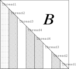
Figure 1: Thread assignment to the Schur complement matrix $B$

The overhead in Algorithm 2 is only in Step 3-2, where only one thread should enter Step 3-2 at a time. Hence, we expected that Algorithm 2 would balance the load better than the simple column-wise distribution employed in SDPARA-C. In particular, the main computation cost of each column $\left[\mbox{\boldmath$B$}\right]_{*j}$ is $\widehat{\mbox{\boldmath$L$}}^{-T}\widehat{\mbox{\boldmath$L$}}\mbox{\boldmath$e$}_{k}$ and $\mbox{\boldmath$N$}^{-T}\mbox{\boldmath$N$}^{-1}\left[\mbox{\boldmath$A$}_{j}\right]_{*k}$; therefore, it is almost proportional to the number of nonzero columns of $\mbox{\boldmath$A$}_{j}$. When only a few of $\mbox{\boldmath$A$}_{1},\ldots,\mbox{\boldmath$A$}_{m}$ have too-many nonzero columns and the others have only a few, a simple column-wise distribution has a hard time keeping the load-balanced. On the other hand, Algorithm 2 can naturally overcome this difficulty.

When we implement Algorithm 2, we should pay attention to the number of threads generated by the BLAS library that CHOLMOD internally calls for the forward/backward substitution ($\widehat{\mbox{\boldmath$L$}}^{-T}\widehat{\mbox{\boldmath$L$}}\mbox{\boldmath$e$}_{k}$ and $\mbox{\boldmath$N$}^{-T}\mbox{\boldmath$N$}^{-1}\left[A_{j}\right]_{*k}$). For example, let us suppose that four cores are available ($u=4$). If we generate four threads in Step 2 and each thread internally generates four threads for the BLAS library, then we need to manage 16 threads in total on the four cores. The overhead for this management is considerable, and when we implemented the multithreaded parallel computing in this way, SDPA-C took at least ten times longer than single-thread computing. Therefore, we decided to turn off the multithreading of the BLAS library before entering the forward/backward substitution routine and turn it on again after the routine finishes.

Now let us examine S-CHOLESKY and P-MATRIX. For S-CHOLESKY, our preliminary experiments indicated that the usage of the BLAS library for both LAPACK and MUMPS is sufficient for delivering the performance of multithreaded parallel computing. In P-MATRIX, the primal auxiliary matrix $\widehat{d\mbox{\boldmath$X$}}$ was evaluated by using formula (40). Since this formula naturally indicates the independence of $\widehat{d\mbox{\boldmath$X$}}$ columns, the simple column-wise distribution was employed in SDPARA-C. However, in multithreading, all of the threads share the memory, hence, we can replace the column-wise distribution with the first-come first-served concept, the same parallel concept as used in Algorithm 2. We also used the above scheme to control the number of threads involved in parallel computing.

Table 2 shows the computation time reduction due to multithreaded parallel computing. It compares the results of SDPA-C 7 with those of SDPA-C 6 and SDPARA-C 1 on the same SDP. In each bottleneck, the upper row is the computation time, and the lower row is the speed-up ratio compared with a single thread.

Table 2: Reduction in computation time due to the multithreaded computing (time in seconds)

	SDPA-C 6	SDPARA-C 1			SDPA-C 7
threads	1	1	2	4	1	2	4
S-ELEMENTS	4873.64	3103.51	1904.64	1309.88	2054.98	1170.37	731.98
		1.00x	1.62x	2.36x	1.00x	1.76x	2.81x
S-CHOLESKY	167.65	312.41	110.76	65.12	161.23	85.24	47.77
		1.00x	2.82x	4.79x	1.00x	1.89x	3.38x
P-MATRIX	346.46	316.04	159.32	81.34	242.06	131.03	83.54
		1.00x	1.98x	3.88x	1.00x	1.85x	2.90x
Other	10.02	32.80	44.76	40.69	21.06	23.88	25.86
Total	5361.77	3764.84	2219.48	1497.03	2479.49	1410.52	889.15
		1.00x	1.63x	2.51x	1.00x	1.76x	2.79x

The table shows that SDPA-C 7 with four threads reduced S-ELEMENTS to 731.98 seconds from 2054.98 seconds on a single thread, a speedup of 2.81-times. The computation time of P-MATRIX also shrank from 242.06 seconds to 83.54 seconds, a speed up of 2.90-times. These time reductions reduced the speed-up in the total time from 2479.49 seconds to 889.15, for a speedup of 2.79-times.

SDPA-C 7 with 4 threads was 6.03-times faster than SDPA-C 6 using only a single thread. The result indicate the parallel schemes discussed above are effectively integrated into MC-PDIPM and the new factorization $\widehat{\mbox{\boldmath$X$}}^{-1}=\widehat{\mbox{\boldmath$L$}}\widehat{\mbox{\boldmath$L$}}^{T}$.

The table also shows that SDPARA-C 1 took longer than SDPA-C 7. This was mainly due to the overhead of the MPI protocol. Since the MPI protocol is designed for multiple PCs, it is not appropriate for a single PC; a multithreaded computation performs better. In addition, Algorithm 2 works more effectively in a multithreaded computing environment than the simple column-wise distribution of SDPARA-C. The speedup of SDPA-C 7 for S-ELEMENTS on four threads was 2.81, and it was higher than that of SDPARA-C 1 (2.36).

4 Numerical Experiments

We conducted a numerical evaluation of the performance of SDPA-C 7. The computing environment was RedHat Linux run on a Xeon X5365 (3.0 GHz, 4 cores) and 48 GB of memory space. We used three groups of test problems, i.e., max-clique problems over lattice graphs, max-cut problems over lattice graphs, and spin-glass problems. In this section, we will use the notation $e$ to denote a vector of all ones, and $\mbox{\boldmath$e$}_{i}$ to denote a vector of all zeros except 1 at the $i$th element.

Max-clique problems over lattice graphs

Consider a graph $G(V,E)$ with the vertex set $V=\{1,\ldots,n\}$ and the edge set $E\subset V\times V$. A vertex subset $S\subset V$ is called a clique if $(i,j)\in E$ for $\forall i\in S,\forall j\in S$. The max-clique problem is to find a clique having the maximum cardinality among all the cliques.

Though the max-clique problem itself is NP-hard, Lovász [17] proposed an SDP relaxation method to obtain a good approximation in polynomial time. The SDP problem below gives a good upper bound of the max-clique cardinality for $G(V,E)$,

$$\max : \mbox{\boldmath$e$}\mbox{\boldmath$e$}^{T}\bullet\mbox{\boldmath$X$}$$

subject to $$: \mbox{\boldmath$I$}\bullet\mbox{\boldmath$X$}=1$$

$$\left(\mbox{\boldmath$e$}_{i}\mbox{\boldmath$e$}_{j}^{T}+\mbox{\boldmath$e$}_{j}\mbox{\boldmath$e$}_{i}^{T}\right)\bullet\mbox{\boldmath$X$}=0\quad\mbox{for}\quad(i,j)\notin E$$

$$\mbox{\boldmath$X$}\succeq\mbox{\boldmath$O$}.$$

For the numerical experiments, we generated SDPs of this type over lattice graphs. A lattice graph $G(V,E)$ is determined by two parameters $p$ and $q$, with the vertex set being $V=\{1,2,\ldots,p\times q\}$ and the edge set $E=\{\left(i+(j-1)\times p,(i+1)+(j-1)\times p\right):i=1,\ldots,p-1,j=1,\ldots,q\}\cup\{\left(i+(j-1)\times p,i+j\times p\right):i=1,\ldots,p,j=1,\ldots,q-1\}$. An example of lattice graphs is shown in Figure 2, where the parameters are $p=4,q=3$.

Figure 2: Lattice graph with the parameters $p=4,q=3$.

We applied the pre-processing technique proposed in [8] to convert the above SDP into an equivalent but sparser SDP. Figure 3 shows the aggregate sparsity pattern $\cal A$ for the max-clique SDP with $p=300,q=10$. We applied approximate minimum degree heuristics to $\cal A$ to make Figure 3, and this figure shows the sparse structure embedded in this SDP. The sizes of cliques $C_{1},\ldots,C_{\ell}$ can be much smaller in comparison with $n=p\times q=300\times 10=3000$, and this $\cal A$ does not incur any fill-in, that is, $\mbox{$\cal E$}=\mbox{$\cal A$}$. This SDP was the example solved in Section 3.

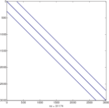
Figure 3: Aggregate sparsity pattern $\cal A$ for the max-clique SDP with $p=300,q=10$.

Max-cut problems over lattice graphs

The SDP relaxation method for solving max-cut problems due to Goemans and Williamson [9] is well-known, and it marked the beginning of studies on SDP relaxation methods. Here, one considers a graph $G(V,E)$ with the vertex set $V=\{1,\ldots,n\}$ and the edge set $E\subset V\times V$. Each edge $(i,j)\in E$ has the corresponding non-negative weight $w_{ij}$ (for simplicity, $w_{ij}=0$ if $(i,j)\notin E$). The weight of the cut $C\subset V$ is the total weight of the edges traversed between $C$ and $V\backslash C$. The max-cut problem is to find a subset $C$ which maximizes the cut weight,

$$\max : \sum_{i\in C,j\in V\backslash C}w_{ij}\qquad\mbox{subject to}\ :\ C\subset V.$$

An SDP relaxation of this problem is given by

$$\min : \mbox{\boldmath$A$}_{0}\bullet\mbox{\boldmath$X$}$$

subject to $$: \left(\mbox{\boldmath$e$}_{i}\mbox{\boldmath$e$}_{i}^{T}\right)\bullet\mbox{\boldmath$X$}=1\quad\mbox{for}\quad i=1,\ldots,n$$

$$\mbox{\boldmath$X$}\succeq\mbox{\boldmath$O$},$$

where $\mbox{\boldmath$A$}_{0}$ is defined by $A_{0}=\left(-\mbox{diag}(\mbox{\boldmath$W$}\mbox{\boldmath$e$})+\mbox{\boldmath$W$}\right)$, $W$ is the matrix whose $(i,j)$ element is $w_{ij}$ for $i=1,\ldots,n,\ j=1,\ldots,n$, and $\mbox{diag}(\mbox{\boldmath$w$})$ is the diagonal matrix whose diagonal elements are the elements of $w$.

When we generate SDP problems from the max-cut problem over the lattice graphs, its aggregate sparsity pattern appears in the coefficient matrix of the objective function $\mbox{\boldmath$A$}_{0}$. Hence, we can find a similar structure to the one shown in Figure 3 in its aggregate sparsity pattern.

Spin-glass problems

The four SDPs of this type were collected as a torus set in the 7th DIMACS benchmark problems [12]. These SDPs arise in computations of the ground-state energy of Ising spin glasses in quantum chemistry. More information on this energy computation can be found at the Spin Glass Server [13] webpage and references therein.

The Ising spin-glass model has a parameter $p$ (the number of samples), and if we generate an SDP from a 3D spin-glass model, the dimension of the variable matrices $X$ and $Y$ is $n=p^{3}$ [13]. Figure 4 illustrates the aggregate sparsity pattern $\cal A$ of the spin-glass SDP with $p=23$ and $n=23^{3}=12167$.

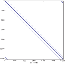
Figure 4: The aggregate sparsity pattern $\cal A$ of the spin-glass SDP with $p=23$.

Table 3 summarizes the SDPs of the numerical experiments. The first column is SDP’s name and the second $p$ is the parameter used to generate it (We fixed the parameter $q$ to $10$ for the max-clique problems and the max-cut problems). The third column $n$ is the dimension of the variable matrices $X$ and $Y$, and the fourth column is the density of aggregate sparsity pattern defined by $\frac{|\mbox{$\cal A$}|}{n^{2}}$. The fifth column $\ell$ is the number of cliques ($C_{1},\ldots,C_{\ell}$), and the sixth and seventh columns are the average and maximum sizes of the cliques defined by $\frac{\sum_{r=1}^{\ell}|C_{r}|}{\ell}$ and $\max_{r=1,\ldots,\ell}C_{r}$, respectively. The eighth column $m$ is the number of input data matrices $\mbox{\boldmath$A$}_{1},\ldots,\mbox{\boldmath$A$}_{m}$.

Table 3: The sizes of the SDPs in the numerical experiments

Name	$p$	$n$	density	$\ell$	ave-size	max-size	$m$
MaxClique300	300	3000	0.38%	348	28.36	51	5691
MaxClique400	400	4000	0.28%	439	29.89	59	7591
MaxClique500	500	5000	0.23%	581	28.26	50	9491
MaxCut400	400	4000	0.15%	1282	8.05	26	4000
MaxCut500	500	5000	0.12%	1607	8.04	26	5000
MaxCut600	600	6000	0.097%	1932	8.04	26	6000
MaxCut800	800	8000	0.072%	2582	8.03	26	8000
MaxCut1000	1000	10000	0.058%	3232	8.02	26	10000
MaxCut1200	1200	12000	0.048%	3882	8.02	26	12000
SpinGlass10	10	1000	0.80%	155	25.69	294	1000
SpinGlass15	15	3375	0.24%	191	29.97	773	3375
SpinGlass18	18	5832	0.13%	1118	28.13	913	5832
SpinGlass20	20	8000	0.10%	1737	25.75	1080	8000
SpinGlass23	23	12167	0.066%	2556	27.30	1488	12167
SpinGlass25	25	15625	0.051%	3173	29.50	1798	15625

We compared the computation times of SDPA-C 6 [20], SDPA-C 7, and SDPA 7 [26] and SeDuMi 1.3 [23]. The former two implemented MC-PDIPM, while the latter two implemented the standard PDIPM. Here, we did not conduct a numerical experiment on SDPARA-C, since we found that the overhead due to the MPI protocol was a severe disadvantage when we ran it on a single PC as shown in Section 3.2.

Table 4 lists the computation times of the four solvers using their default parameters. We used four threads for SDPA-C 7 and SDPA 7. The symbol ’$>$2days’ in the table indicates that we gave up on the SeDuMi execution since it required at least two days.

Table 4: Computation times of four solvers for the SDPs in Table 3 (time in seconds)

Name	SDPA-C6	SDPA-C7	SDPA 7	SeDuMi1.3
MaxClique300	4792.28	889.15	11680.12	10260.15
MaxClique400	12681.16	1903.13	26159.40	24824.05
MaxClique500	19973.98	3733.41	38265.02	46168.56
MaxCut400	386.80	539.22	3686.78	16779.68
MaxCut500	683.27	876.81	6548.26	32557.13
MaxCut600	1194.89	1295.01	11098.35	60444.33
MaxCut800	2518.80	2371.43	25377.62	146235.81
MaxCut1000	4301.11	4032.80	47270.45	$>$2days
MaxCut1200	7400.28	6030.00	75888.85	$>$2days
SpinGlass10	50.10	20.77	11.85	228.71
SpinGlass15	1306.00	560.40	336.40	13789.58
SpinGlass18	6734.40	2136.88	1522.60	68570.89
SpinGlass20	15450.13	4552.10	3726.03	$>$2days
SpinGlass23	55942.57	13184.25	12598.14	$>$2days
SpinGlass25	107502.48	24913.20	26023.67	$>$2days

On the max-clique problems, the MC-PDIPM solvers were faster than the standard PDIPM solvers. Since the matrix-completion method benefited from the nice properties of lattice graphs, even SDPA-C 6 was twice as faster as SDPA 7. The detailed breakdown of the time on MaxClique400 is displayed in Table 5 (since SeDuMi does not print out its internal computation time, we did not list its breakdown). As shown in the SDPA 7 column, the standard PDIPM took a long time on P-MATRIX (17) and Other (mainly, the computation of the step length by (15)). Though these parts required an $O(n^{3})$ computation cost, the MC-PDIPM decomposed the full matrix $X$ into the sub-matrices $\overline{\mbox{\boldmath$X$}}_{C_{r}C_{r}}\ (r=1,\ldots,\ell)$; hence, it was able to reduce the computation cost of these two parts. Furthermore, SDPA-C 7 resolved the heaviest parts of SDPA-C 6 by using the new factorization $\widehat{\mbox{\boldmath$X$}}^{-1}=\widehat{\mbox{\boldmath$L$}}\widehat{\mbox{\boldmath$L$}}^{T}$ and multithreaded parallel computing. Consequently, SDPA-C 7 was the fastest among the four solvers; in particular, it was 12.36-times faster than SeDuMi on MaxClique500.

Table 5: Computation times on MaxClique400 (time in seconds)

	SDPA-C 6	SDPA-C 7	SDPA 7	SeDuMi 1.3
S-ELEMENTS	9314.34	1431.69	262.04	–
S-CHOLESKY	2601.04	248.55	403.28	–
P-MATRIX	734.41	175.24	13151.10	–
Other	31.37	47.65	12342.98	–
Total	12681.16	1903.13	26159.40	24824.05

For the max-cut problems, though MC-PDIPM was again superior to the standard PDIPM, SDPA-C 7 was less effective than SDPA-C 6. In particular, it took longer on S-ELEMENTS and P-MATRIX, both of which utilized multithreaded computing. It needed an overhead to generate the threads, and the input matrices of the max-cut problems were too simple to derive any benefit from multithreaded computing. Indeed, each input matrix $\mbox{\boldmath$A$}_{i}=\mbox{\boldmath$e$}_{i}\mbox{\boldmath$e$}_{i}^{T}$ has only one nonzero element, and this is reflected in the short computation time of SDPA 7’s S-ELEMENTS. In the standard PDIPM, the S-ELEMENTS computation is an inexpensive task of (18) with $\mbox{\boldmath$A$}_{i}=\mbox{\boldmath$e$}_{i}\mbox{\boldmath$e$}_{i}^{T}$ and $\mbox{\boldmath$A$}_{j}=\mbox{\boldmath$e$}_{j}\mbox{\boldmath$e$}_{j}^{T}$, since the fully dense matrices $X$ and $\mbox{\boldmath$Y$}^{-1}$ are obtained with extensive memory space and a heavy computation through P-MATRIX and the inverse of the fully dense matrix. For the large max-cut problems, however, SDPA-C 7 solved the SDPs faster than SDPA-C 6 or SDPA 7. As shown in the Max1200 result of Table 6, SDPA-C 7 still incurred a multithreading overhead on S-ELEMENTS and P-MATRIX, but the multithreaded BLAS library resolved the principal bottleneck, S-CHOLESKY. We can say that SDPA-C 7 would work even better on larger SDPs of this type.

Table 6: Computation times on MaxCut500 and MaxCut1200 (time in seconds)

MaxCut500
	SDPA-C 6	SDPA-C 7	SDPA 7	SeDuMi 1.3
S-ELEMENTS	105.25	317.56	16.17	–
S-CHOLESKY	502.43	226.06	214.43	–
P-MATRIX	61.21	315.73	3254.05	–
Other	14.38	17.46	3063.60	–
Total	683.27	876.81	6548.26	32557.13
MaxCut1200
	SDPA-C 6	SDPA-C 7	SDPA 7	SeDuMi 1.3
S-ELEMENTS	1265.02	1800.27	107.17	–
S-CHOLESKY	5562.48	2318.17	2674.50	–
P-MATRIX	532.21	1837.53	39490.81	–
Other	40.57	74.03	33616.37	–
Total	7400.28	6030.00	75888.85	$>$2days

SDPA 7 was the fastest in solving the spin-glass SDPs with $p=10$, since its standard PDIPM is more effective on smaller SDPs where the variable matrices are small and do not need to be decomposed. When we increased $p$, however, the time difference between SDPA-C 7 and SDPA 7 shrank, and SDPA-C 7 became faster than SDPA 7 at $p=25$. The reason why the growth in the computation time of SDPA-C 7 was not as steep in comparison with SDPA 7 is that the average size of cliques does not grow with $p$, as shown in Table 3. In particular, as seen in the breakdown of the computation times in Table 7, this affects P-MATRIX and its computation time in MC-PDIPM grows more gradually than in the standard PDIPM. SpinGlass25 was the largest among the spin-glass SDPs in our experiments; it required almost 48 GB of memory, close to the capacity of our computing environment. We expect that SDPA-C 7 would be more effective on larger SDPs of the spin-glass type. The ratios of SpinGlass25 over SpinGlass23 were $\frac{107502.48}{55942.57}=1.92$ in SDPA-C 6, $\frac{24913.20}{13184.25}=1.89$ in SDPA-C 7, and $\frac{26023.67}{12598.14}=2.07$ in SDPA 7. In addition, SDPA 7 incurred a considerable computation cost on the other parts, i.e., ’Other’. This ’Other’ category in SDPA 7 contained the miscellaneous parts related to the computation of the variable matrices $X$ and $Y$. Since they are miscellaneous and we can not say which costs the most, we did not examine them in detail, but we note that the fully dense properties of $X$ and $Y$ diminished the performance of the ’Other’ parts of SDPA 7.

We should emphasize that MC-PDIPM is not the only reason for SDPA-C 7 being faster, because Table 7 shows that SDPA-C 6 was much slower than SDPA 7. The new factorization of $\widehat{\mbox{\boldmath$X$}}^{-1}=\widehat{\mbox{\boldmath$L$}}\widehat{\mbox{\boldmath$L$}}^{T}$ and the multithreaded computing were the keys to solving the spin-glass SDPs in the shortest time.

Table 7: Computation times on Spinglass18 and Spinglass25 (time in seconds)

Spinglass18
	SDPA-C 6	SDPA-C 7	SDPA 7	SeDuMi 1.3
S-ELEMENTS	2738.18	1012.13	22.93	–
S-CHOLESKY	178.15	52.70	30.69	–
P-MATRIX	2516.52	984.76	620.54	–
Other	1301.5	87.29	848.44	–
Total	6734.40	2136.88	1522.60	68570.89
Spinglass25
	SDPA-C 6	SDPA-C 7	SDPA 7	SeDuMi 1.3
S-ELEMENTS	35314.96	11829.56	220.19	–
S-CHOLESKY	3681.44	945.49	520.39	–
P-MATRIX	45238.37	11594.76	11846.59	–
Other	23267.71	588.39	13436.50	–
Total	107502.48	24913.20	26023.67	$>$2days

Finally, Table 8 shows the amount of memory required to solve the SDPs in Tables 5, 6, and 7. The notation ’$>$ 31G’ indicates that SeDuMi exceeded the time limit (2 days) and used 31 gigabytes of memory during the two-day execution. By comparison, MC-PDIPM saved a lot of memory by removing the fully dense matrices. For example, in MaxClique400, SDPA-C7 used only $\frac{1}{6}$ times and $\frac{1}{10}$ times the memory of SDPA7 and SeDuMi, respectively. In addition, the new factorization reduced the memory needed for the largest SDP (Spinglass25) from 8.1 gigabytes in SDPA-C6 to 3.7 gigabytes in SDPA-C7. It reduced the required memory because it can reuse the memory structure of CHOLMOD.

Table 8: Amount of memory space required for solving SDPs in Tables 5, 6, and 7 (M and G indicate megabytes and gigabytes.)

Name	SDPA-C6	SDPA-C7	SDPA 7	SeDuMi1.3
MaxClique400	548M	516M	3.0G	5.2G
MaxCut500	249M	236M	4.1G	6.1G
MaxCut1200	1.2G	1.2G	23G	$>$ 31G
SpinGlass18	2.0G	707M	5.6G	8.3G
SpinGlass25	8.1G	3.7G	40G	$>$ 36G

5 Conclusions and Future Directions

We implemented a new SDPA-C 7, that uses a more effective factorization of $\widehat{\mbox{\boldmath$X$}}^{-1}=\widehat{\mbox{\boldmath$L$}}\widehat{\mbox{\boldmath$L$}}^{T}$ and takes advantages of multithreaded parallel computing. Our numerical experiments verified that these two improvements enhanced the performance of MC-PDIPM and reduced the computation times of the max-clique and spin-glass SDPs.

SDPA-C 7 is available at the SDPA web site, http://sdpa.sourceforge.net/. Unlike SDPA-C 6, SDPA-C 7 has a callable library and a Matlab interface; it can now be embedded in other C++ software packages and be directly called from inside Matlab. The callable library and Matlab interface will no doubt expand the usage of SDPA-C.

As shown in the numerical experiments on the max-cut problems, if the input SDP has a very simple structure, we should automatically turn off the multithreading. However, this would require a complex task to estimate the computation time accurately over the multiple threads from the input SDPs. Another point is that SDPA-C 7 has a tendency to be faster for large SDPs. This is an excellent feature, but it does not extend to smaller SDPs. Although this is mainly because MC-PDIPM is intended to solve large SDPs with the factorization of the variable matrices, we should combine it with other methods that effectively compute the forward/backward substitution of small dimensions.

References

- [1] F. Alizadeh, J.-P. A. Haeberly, and M. L. Overton. Primal-dual interior-point methods for semidefinite programming: Convergence rates, stability and numerical results. SIAM J. Optim., 8(2):746–768, 1998.
- [2] P. R. Amestoy, I. S. Duff, and J. Y. L’Excellent. Multifrontal parallel distributed symmetric and unsymmetric solvers. Comput. Methods Appl. Mech. Eng., 184:501–520, 2000.
- [3] E. Anderson, Z. Bai, C. Bischof, S. Blackford, J. Demmel, J. Dongarra, J. Croz, A. Greenbaum, S. Hammarling, A.McKenney, and D. Sorensen. LAPACK Users’ Guide Third. Society for Industrial and Applied Mathematics, Philadelphia, PA, USA, 1999.
- [4] P. Biswas and Y. Ye. Semidefinite programming for ad-hoc wireless sensor network localization. In Proceedings of the third international symposium on information processing in sensor networks, Berkeley, California, 2004. ACM.
- [5] B. Borchers. CSDP, a C library for semidefinite programming. Optim. Methods Softw., 11 & 12(1-4):613–623, 1999.
- [6] Y. Chen, T. A. Davis, W. W. Hager, and S. Rajamanickam. Algorithm 887: CHOLMOD: supernodal sparse Cholesky factorization and update/downdate. ACM Trans. Math. Softw., 35(3):Article No. 22, 2009.
- [7] M. Fukuda, B. J. Braams, M. Nakata, M. L. Overton, J. K. Percus, M. Yamashita, and Z. Zhao. Large-scale semidefinite programs in electronic structure calculation. Math. Program. Series B, 109(2-3):553–580, 2007.
- [8] M. Fukuda, M. Kojima, K. Murota, and K. Nakata. Exploiting sparsity in semidefinite programming via matrix completion I: general framework. SIAM J. Optim., 11(3):647–674, 2000.
- [9] M. X. Goemans and D. P. Williamson. Improved approximation algorithms for maximum cut and satisfiability problems using semidefinite programming. J. Assoc. Comput. Mach., 42(6):1115–1145, 1995.
- [10] R. Grone, C. R. Johnson, E. M. Sá, and H. Wolkowicz. Positive definite completions of partial hermitian matrices. Linear Algebra Appl., 58:109–124, 1984.
- [11] C. Helmberg, F. Rendl, R. J. Vanderbei, and H. Wolkowicz. An interior-point method for semidefinite programming. SIAM J. Optim., 6(2):342–361, 1996.
- [12] D. Johnson and G. Pataki, 2000. http://dimacs.rutgers.edu/Challenges/Seventh/.
- [13] M. Jünger, 2011. http://www.informatik.uni-koeln.de/spinglass/.
- [14] S. Kim, M. Kojima, H. Waki, and M. Yamashita. Algorithm 920: SFSDP: a Sparse version of Full SemiDefinite Programming relaxation for sensor network localization problems. ACM Trans. Math. Softw., 38(4):Article No. 27, 2012.
- [15] M. Kojima, S. Shindoh, and S. Hara. Interior-point methods for the monotone semidefinite linear complementarity problems in symmetric matrices. SIAM J. Optim., 7:86–125, 1997.
- [16] C. L. Lawson, R. J. Hanson, D. Kincaid, and F. T. Krogh. Basic linear algebra subprograms for fortran usage. ACM Trans. Math. Softw., 5:308—323, 1979.
- [17] L. Lovász. On the shannon capacity of a graph. IEEE Trans. Inf. Theory, 25:1–7, 1979.
- [18] R. D. C. Monteiro. Primal-dual path-following algorithms for semidefinite programming. SIAM J. Optim., 7(3):663–678, 1997.
- [19] K. Nakata, K. Fujisawa, M. Fukuda, M. Kojima, and K. Murota. Exploiting sparsity in semidefinite programming via matrix completion II: implementation and numerical results. Math. Program., Ser B, 95:303–327, 2003.
- [20] K. Nakata, M. Yamashita, K. Fujisawa, and M. Kojima. A parallel primal-dual interior-point method for semidefinite programs. Parallel Computing, 32(1):24–43, 2006.
- [21] M. Nakata, H. Nakatsuji, M. Ehara, M. Fukuda, K. Nakata, and K. Fujisawa. Variational calculations of fermion second-order reduced density matrices by semidefinite programming algorithm. J. Chem. Phys., 114:8282–8292, 2001.
- [22] Y. E. Nesterov and M. J. Todd. Primal-dual interior-point methods for self-scaled cones. SIAM J. Optim., 8(2):324–364, 1998.
- [23] J. F. Sturm. Using SeDuMi 1.02, a MATLAB toolbox for optimization over symmetric cones. Optim. Methods Softw., 11 & 12(1-4):625–653, 1999.
- [24] M.J. Todd. Semidefinite optimization. Acta Numerica, 10:515–560, 2001.
- [25] K.-C. Toh, M. J. Todd, and R. H. Tütüncü. SDPT3 – a MATLAB software package for semidefinite programming, version 1.3. Optim. Methods Softw., 11 & 12(1-4):545–581, 1999.
- [26] M. Yamashita, K. Fujisawa, M. Fukuda, K. Kobayashi, K. Nakta, and M. Nakata. Latest developments in the SDPA family for solving large-scale SDPs. In M. F. Anjos and J. B. Lasserre, editors, Handbook on Semidefinite, Cone and Polynomial Optimization: Theory, Algorithms, Software and Applications, chapter 24, pages 687–714. Springer, NY, USA, 2011.
- [27] M. Yamashita, K. Fujisawa, M. Fukuda, K. Nakata, and M. Nakata. Algorithm 925: Parallel solver for semidefinite programming problem having sparse Schur complement matrix. ACM Trans. Math. Softw., 39(1), 2012. Article No.6.
- [28] M. Yamashita, K. Fujisawa, and M. Kojima. SDPARA: SemiDefinite Programming Algorithm paRAllel version. Parallel Comput., 29(8):1053–1067, 2003.