IC3 Modulo Theories via
Implicit Predicate Abstraction

Abstract

We present a novel approach for generalizing the IC3 algorithm for invariant checking from finite-state to infinite-state transition systems, expressed over some background theories. The procedure is based on a tight integration of IC3 with Implicit (predicate) Abstraction, a technique that expresses abstract transitions without computing explicitly the abstract system and is incremental with respect to the addition of predicates. In this scenario, IC3 operates only at the Boolean level of the abstract state space, discovering inductive clauses over the abstraction predicates. Theory reasoning is confined within the underlying SMT solver, and applied transparently when performing satisfiability checks. When the current abstraction allows for a spurious counterexample, it is refined by discovering and adding a sufficient set of new predicates. Importantly, this can be done in a completely incremental manner, without discarding the clauses found in the previous search.

The proposed approach has two key advantages. First, unlike current SMT generalizations of IC3, it allows to handle a wide range of background theories without relying on ad-hoc extensions, such as quantifier elimination or theory-specific clause generalization procedures, which might not always be available, and can moreover be inefficient. Second, compared to a direct exploration of the concrete transition system, the use of abstraction gives a significant performance improvement, as our experiments demonstrate.

1 Introduction

IC3 [5] is an algorithm for the verification of invariant properties of transition systems. It builds an over-approximation of the reachable state space, using clauses obtained by generalization while disproving candidate counterexamples. In the case of finite-state systems, the algorithm is implemented on top of Boolean SAT solvers, fully leveraging their features. IC3 has demonstrated extremely effective, and it is a fundamental core in all the engines in hardware verification.

There have been several attempts to lift IC3 to the case of infinite-state systems, for its potential applications to software, RTL models, timed and hybrid systems, although the problem is in general undecidable. These approaches are set in the framework of Satisfiability Modulo Theory (SMT) [1] and hereafter are referred to as IC3 Modulo Theories [7, 17, 15, 24]: the infinite-state transition system is symbolically described by means of SMT formulas, and an SMT solver plays the same role of the SAT solver in the discrete case. The key difference is the need in IC3 Modulo Theories for specific theory reasoning to deal with candidate counterexamples. This led to the development of various techniques, based on quantifier elimination or theory-specific clause generalization procedures. Unfortunately, such extensions are typically ad-hoc, and might not always be applicable in all theories of interest. Furthermore, being based on the fully detailed SMT representation of the transition systems, some of these solutions (e.g. based on quantifier elimination) can be highly inefficient.

We present a novel approach to IC3 Modulo Theories, which is able to deal with infinite-state systems by means of a tight integration with predicate abstraction (PA) [11], a standard abstraction technique that partitions the state space according to the equivalence relation induced by a set of predicates. In this work, we leverage Implicit Abstraction (IA) [22], which allows to express abstract transitions without computing explicitly the abstract system, and is fully incremental with respect to the addition of new predicates. In the resulting algorithm, called IC3+IA, the search proceeds as if carried out in an abstract system induced by the set of current predicates $\mathbb{P}$ – in fact, IC3+IA only generates clauses over $\mathbb{P}$. The key insight is to exploit IA to obtain an abstract version of the relative induction check. When an abstract counterexample is found, as in Counter-Example Guided Abstraction-Refinement (CEGAR), it is simulated in the concrete space and, if spurious, the current abstraction is refined by adding a set of predicates sufficient to rule it out.

The proposed approach has several advantages. First, unlike current SMT generalizations of IC3, IC3+IA allows to handle a wide range of background theories without relying on ad-hoc extensions, such as quantifier elimination or theory-specific clause generalization procedures. The only requirement is the availability of an effective technique for abstraction refinement, for which various solutions exist for many important theories (e.g. interpolation [14], unsat core extraction, or weakest precondition). Second, the analysis of the infinite-state transition system is now carried out in the abstract space, which is often as effective as an exact analysis, but also much faster. Finally, the approach is completely incremental, without having to discard or reconstruct clauses found in the previous iterations.

We experimentally evaluated IC3+IA on a set of benchmarks from heterogeneous sources [2, 13, 17], with very positive results. First, our implementation of IC3+IA is significantly more expressive than the SMT-based IC3 of [7], being able to handle not only the theory of Linear Rational Arithmetic (LRA) like [7], but also those of Linear Integer Arithmetic (LIA) and fixed-size bit-vectors (BV). Second, in terms of performance IC3+IA proved to be uniformly superior to a wide range of alternative techniques and tools, including state-of-the-art implementations of the bit-level IC3 algorithm ([10, 21, 3]), other approaches for IC3 Modulo Theories ([7, 15, 17]), and techniques based on k-induction and invariant discovery ([13, 16]). A remarkable property of IC3+IA is that it can deal with a large number of predicates: in several benchmarks, hundreds of predicates were introduced during the search. Considering that an explicit computation of the abstract transition relation (e.g. based on All-SMT [18]) often becomes impractical with a few dozen predicates, we conclude that IA is fundamental to scalability, allowing for efficient reasoning in a fine-grained abstract space.

The rest of the paper is structured as follows. In Section 2 we present some background on IC3 and Implicit Abstraction. In Section 3 we describe IC3+IA and prove its formal properties. In Section 4 we discuss the related work. In Section 5 we experimentally evaluate our method. In Section 6 we draw some conclusions and present directions for future work.

2 Background

2.1 Transition Systems

Our setting is standard first order logic. We use the standard notions of theory, satisfiability, validity, logical consequence. We denote formulas with $\varphi,\psi,I,T,P$, variables with $x$, $y$, and sets of variables with $X$, $Y$, $\overline{X}$, $\widehat{X}$. Unless otherwise specified, we work on quantifier-free formulas, and we refer to 0-arity predicates as Boolean variables, and to 0-arity uninterpreted functions as (theory) variables. A literal is an atom or its negation. A clause is a disjunction of literals, whereas a cube is a conjunction of literals. If $s$ is a cube $l_{1}\land\ldots\land l_{n}$, with $\neg s$ we denote the clause $\neg l_{1}\lor\ldots\lor\neg l_{n}$, and vice versa. A formula is in conjunctive normal form (CNF) if it is a conjunction of clauses, and in disjunctive normal form (DNF) if it is a disjunction of cubes. With a little abuse of notation, we might sometimes denote formulas in CNF $C_{1}\land\ldots\land C_{n}$ as sets of clauses $\{C_{1},\ldots,C_{n}\}$, and vice versa. If $X_{1},\ldots,X_{n}$ are a sets of variables and $\varphi$ is a formula, we might write $\varphi(X_{1},\ldots,X_{n})$ to indicate that all the variables occurring in $\varphi$ are elements of $\bigcup_{i}X_{i}$. For each variable $x$, we assume that there exists a corresponding variable $x^{\prime}$ (the primed version of $x$). If $X$ is a set of variables, $X^{\prime}$ is the set obtained by replacing each element $x$ with its primed version ($X^{\prime}=\{x^{\prime}\mid x\in X\}$), $\overline{X}$ is the set obtained by replacing each $x$ with $\overline{x}$ ($\overline{X}=\{\overline{x}\mid x\in X\}$) and $X^{n}$ is the set obtained by adding $n$ primes to each variable ($X^{n}=\{x^{n}\mid x\in X\}$).

Given a formula $\varphi$, $\varphi^{\prime}$ is the formula obtained by adding a prime to each variable occurring in $\varphi$. Given a theory T, we write $\varphi\models_{T}\psi$ (or simply $\varphi\models\psi$) to denote that the formula $\psi$ is a logical consequence of $\varphi$ in the theory T.

A transition system $S$ is a tuple $S=\langle{X,I,T}\rangle$ where $X$ is a set of (state) variables, $I(X)$ is a formula representing the initial states, and $T(X,X^{\prime})$ is a formula representing the transitions. A state of $S$ is an assignment to the variables $X$. A path of $S$ is a finite sequence $s_{0},s_{1},\ldots,s_{k}$ of states such that $s_{0}\models I$ and for all $i$, $0\leq i<k$, $s_{i},s^{\prime}_{i+1}\models T$.

Given a formula $P(X)$, the verification problem denoted with $S\models P$ is the problem to check if for all paths $s_{0},s_{1},\ldots,s_{k}$ of $S$, for all $i$, $0\leq i\leq k$, $s_{i}\models P$. Its dual is the reachability problem, which is the problem to find a path $s_{0},s_{1},\ldots,s_{k}$ of $S$ such that $s_{k}\models\neg P$. $P(X)$ represents the “good” states, while $\neg P$ represents the “bad” states.

Inductive invariants are central to solve the verification problem. $P$ is an inductive invariant iff (i) $I(X)\models P(X)$; and (ii) $P(X)\land T(X,X^{\prime})\models P(X^{\prime})$. A weaker notion is given by relative inductive invariants: given a formula $\phi(X)$, $P$ is inductive relative to $\phi$ iff (i) $I(X)\models P(X)$; and (ii) $\phi(X)\land P(X)\land T(X,X^{\prime})\models P(X^{\prime})$.

2.2 IC3 with SMT

IC3 [5] is an efficient algorithm for the verification of finite-state systems, with Boolean state variables and propositional logic formulas. IC3 was subsequently extended to the SMT case in [7, 15]. In the following, we present its main ideas, following the description of [7]. For brevity, we have to omit several important details, for which we refer to [5, 7, 15].

Let $S$ and $P$ be a transition system and a set of good states as in §2.1. The IC3 algorithm tries to prove that $S\models P$ by finding a formula $F(X)$ such that: (i) $I(X)\models F(X)$; (ii) $F(X)\land T(X,X^{\prime})\models F(X^{\prime})$; and (iii) $F(X)\models P(X)$.

In order to construct an inductive invariant $F$, IC3 maintains a sequence of formulas (called trace) $F_{0}(X),\ldots,F_{k}(X)$ such that: (i) $F_{0}=I$; (ii) $F_{i}\models F_{i+1}$; (iii) $F_{i}(X)\land T(X,X^{\prime})\models F_{i+1}(X^{\prime})$; (iv) for all $i<k$, $F_{i}\models P$. Therefore, each element of the trace $F_{i+1}$, called frame, is inductive relative to previous one, $F_{i}$. IC3 strengthens the frames by finding new relative inductive clauses by checking the unsatisfiability of the formula:

$$RelInd(F,T,c):=F\land c\land T\land\neg c^{\prime}.$$ (1)

More specifically, the algorithm proceeds incrementally, by alternating two phases: a blocking phase, and a propagation phase. In the blocking phase, the trace is analyzed to prove that no intersection between $F_{k}$ and $\neg P(X)$ is possible. If such intersection cannot be disproved on the current trace, the property is violated and a counterexample can be reconstructed. During the blocking phase, the trace is enriched with additional formulas, which can be seen as strengthening the approximation of the reachable state space. At the end of the blocking phase, if no violation is found, $F_{k}\models P$.

The propagation phase tries to extend the trace with a new formula $F_{k+1}$, moving forward the clauses from preceding $F_{i}$’s. If, during this process, two consecutive frames become identical (i.e. $F_{i}=F_{i+1}$), then a fixpoint is reached, and IC3 terminates with $F_{i}$ being an inductive invariant proving the property.

In the blocking phase IC3 maintains a set of pairs $(s,i)$, where $s$ is a set of states that can lead to a bad state, and $i>0$ is a position in the current trace. New formulas (in the form of clauses) to be added to the current trace are derived by (recursively) proving that a set $s$ of a pair $(s,i)$ is unreachable starting from the formula $F_{i-1}$. This is done by checking the satisfiability of the formula $RelInd(F_{i-1},T,\neg{s})$. If the formula is unsatisfiable, then $\neg s$ is inductive relative to $F_{i-1}$, and IC3 strengthens $F_{i}$ by adding $\neg s$ to it, thus blocking the bad state $s$ at $i$. If, instead, (1) is satisfiable, then the overapproximation $F_{i-1}$ is not strong enough to show that $s$ is unreachable. In this case, let $p$ be a subset of the states in $F_{i-1}\land\neg s$ such that all the states in $p$ lead to a state in $s^{\prime}$ in one transition step. Then, IC3 continues by trying to show that $p$ is not reachable in one step from $F_{i-2}$ (that is, it tries to block the pair $(p,i-1)$). This procedure continues recursively, possibly generating other pairs to block at earlier points in the trace, until either IC3 generates a pair $(q,0)$, meaning that the system does not satisfy the property, or the trace is eventually strengthened so that the original pair $(s,i)$ can be blocked.

A key difference between the original Boolean IC3 and its SMT extensions in [7, 15] is in the way sets of states to be blocked or generalized are constructed. In the blocking phase, when trying to block a pair $(s,i)$, if the formula (1) is satisfiable, then a new pair $(p,i-1)$ has to be generated such that $p$ is a cube in the preimage of $s$ wrt. $T$. In the propositional case, $p$ can be obtained from the model $\mu$ of (1) generated by the SAT solver, by simply dropping the primed variables occurring in $\mu$. This cannot be done in general in the first-order case, where the relationship between the current state variables $X$ and their primed version $X^{\prime}$ is encoded in the theory atoms, which in general cannot be partitioned into a primed and an unprimed set. The solution proposed in [7] is to compute $p$ by existentially quantifying (1) and then applying an under-approximated existential elimination algorithm for linear rational arithmetic formulas. Similarly, in [15] a theory-aware generalization algorithm for linear rational arithmetic (based on interpolation) was proposed, in order to strengthen $\neg s$ before adding it to $F_{i}$ after having successfully blocked it.

2.3 Implicit Abstraction

2.3.1 Predicate abstraction

Abstraction [9] is used to reduce the search space while preserving the satisfaction of some properties such as invariants. If $\widehat{S}$ is an abstraction of $S$, if a condition is reachable in $S$, then also its abstract version is reachable in $\widehat{S}$. Thus, if we prove that a set of states is not reachable in $\widehat{S}$, the same can be concluded for the concrete transition system $S$.

In Predicate Abstraction [11], the abstract state-space is described with a set of predicates. Given a TS $S$, we select a set $\mathbb{P}$ of predicates, such that each predicate $p\in\mathbb{P}$ is a formula over the variables $X$ that characterizes relevant facts of the system. For every $p\in\mathbb{P}$, we introduce a new abstract variable $x_{p}$ and define $X_{\mathbb{P}}$ as $\{x_{p}\}_{p\in\mathbb{P}}$. The abstraction relation $H_{\mathbb{P}}$ is defined as $\textit{H}_{\mathbb{P}}(X,X_{\mathbb{P}}):=\bigwedge_{p\in\mathbb{P}}x_{p}\leftrightarrow p(X)$. Given a formula $\phi(X)$, the abstract version $\widehat{\phi}_{\mathbb{P}}$ is obtained by existentially quantifying the variables $X$, i.e., $\widehat{\phi}_{\mathbb{P}}=\exists X.(\phi(X)\wedge\textit{H}_{\mathbb{P}}(X,X_{\mathbb{P}}))$. Similarly for a formula over $X$ and $X^{\prime}$, $\widehat{\phi}_{\mathbb{P}}=\exists X,X^{\prime}.(\phi(X,X^{\prime})\wedge\textit{H}_{\mathbb{P}}(X,X_{\mathbb{P}})\wedge\textit{H}_{\mathbb{P}}(X^{\prime},X_{\mathbb{P}}^{\prime}))$. The abstract system with $\widehat{S}_{\mathbb{P}}=\langle{X_{\mathbb{P}},\widehat{I}_{\mathbb{P}},\widehat{T}_{\mathbb{P}}}\rangle$ is obtained by abstracting the initial and the transition conditions. In the following, when clear from the context, we write just $\widehat{\phi}$ instead of $\widehat{\phi}_{\mathbb{P}}$.

Since most model checkers deal only with quantifier-free formulas, the computation of $\widehat{S}_{\mathbb{P}}$ requires the elimination of the existential quantifiers. This may result in a bottleneck and some techniques compute weaker/more abstract systems (cfr., e.g., [20]).

2.3.2 Implicit predicate abstraction

Figure 1: Abstract path.

Implicit predicate abstraction [22] embeds the definition of the predicate abstraction in the encoding of the path. This is based on the following formula:

$$\textit{EQ}_{\mathbb{P}}(X,\overline{X}):=\bigwedge_{p\in\mathbb{P}}p(X)\leftrightarrow p(\overline{X})\vspace{-2mm}$$ (2)

which relate two concrete states corresponding to the same abstract state. The formula $\widehat{\textit{Path}}_{k,\mathbb{P}}:=\bigwedge_{1\leq h<k}(T(\overline{X}^{h-1},X^{h})\wedge\textit{EQ}_{\mathbb{P}}(X^{h},\overline{X}^{h}))\wedge T(\overline{X}^{k-1},X^{k})$ is satisfiable iff there exists a path of $k$ steps in the abstract state space. Intuitively, instead of having a contiguous sequence of transitions, the encoding represents a sequence of disconnected transitions where every gap between two transitions is forced to lay in the same abstract state (see Fig. 1). $\text{BMC}^{k}_{\mathbb{P}}$ encodes the abstract bounded model checking problem and is obtained from $\widehat{\textit{Path}}_{k,\mathbb{P}}$ by adding the abstract initial and target conditions: $\text{BMC}^{k}_{\mathbb{P}}=I(X^{0})\wedge\textit{EQ}_{\mathbb{P}}(X^{0},\overline{X}^{0})\wedge\widehat{\textit{Path}}_{k,\mathbb{P}}\wedge\textit{EQ}_{\mathbb{P}}(X^{k},\overline{X}^{k})\wedge{\neg P}(\overline{X}^{k})$.

3 IC3 with Implicit Abstraction

3.1 Main idea

The main idea of IC3+IA is to mimic how IC3 would work on the abstract state space defined by a set of predicates $\mathbb{P}$, but using IA to avoid quantifier elimination to compute the abstract transition relation. Therefore, clauses, frames and cubes are restricted to have predicates in $\mathbb{P}$ as atoms. We call these clauses, frames and cubes respectively $\mathbb{P}$-clauses, $\mathbb{P}$-formulas, and $\mathbb{P}$-cubes. Note that for any $\mathbb{P}$-formula $\phi$ (and thus also for $\mathbb{P}$-cubes and $\mathbb{P}$-clauses), $\widehat{\phi}=\phi[X_{\mathbb{P}}/\mathbb{P}]\wedge\exists X.(\bigwedge_{p\in\mathbb{P}}x_{p}\leftrightarrow p(X))$, and thus $\widehat{(\neg\phi)}=\neg\widehat{(\phi)}$.

The key point of IC3+IA is to use an abstract version of the check (1) to prove that an abstract clause $\widehat{c}$ is inductive relative to the abstract frame $\widehat{F}$:

$$AbsRelInd(F,T,c,\mathbb{P}) := F(X)\land c(X)\land$$ (3)

$$\textit{EQ}_{\mathbb{P}}(X,\overline{X})\land T(\overline{X},\overline{X}^{\prime})\land\textit{EQ}_{\mathbb{P}}(\overline{X}^{\prime},X^{\prime})\land\neg c(X^{\prime})$$

Theorem 3.1

Consider a set $\mathbb{P}$ of predicates, $\mathbb{P}$-formulas $F$ and a $\mathbb{P}$-clause $c$. $RelInd(\widehat{F},\widehat{T},\widehat{c})$ is satisfiable iff $AbsRelInd(F,T,c,\mathbb{P})$ is satisfiable. In particular, if $s\models AbsRelInd(F,T,c,\mathbb{P})$, then $\widehat{s}\models RelInd(\widehat{F},\widehat{T},\widehat{c})$.

Proof

Suppose $s\models AbsRelInd(F,T,c,\mathbb{P})$. Let us denote with $\overline{t}$ and ${t}$ the projections of $s$ respectively over $\overline{X}\cup\overline{X}^{\prime}$ and over $X\cup X^{\prime}$. Then $\overline{t}\models T$ and therefore $\widehat{\overline{t}}\models\widehat{T}$. Since $s\models\textit{EQ}_{\mathbb{P}}(X,\overline{X})\wedge\textit{EQ}_{\mathbb{P}}(\overline{X}^{\prime},X^{\prime})$, $\widehat{t}$ and $\widehat{\overline{t}}$ are the same abstract transition and therefore $\widehat{{t}}\models\widehat{T}$. Since $t\models F\wedge c$, then $\widehat{t}\models\widehat{F}\wedge\widehat{c}$. Since $t\models\neg c^{\prime}$, then $\widehat{t}\models\widehat{(\neg c^{\prime})}$ and since $c$ is a Boolean combinations of $\mathbb{P}$, then $\widehat{t}\models\neg\widehat{c}^{\prime}$. Thus, $\widehat{s}\models\widehat{t}\models RelInd(\widehat{F},\widehat{T},\widehat{c})$.

For the other direction, suppose $\overline{t}\models RelInd(\widehat{F},\widehat{T},\widehat{c})$. Then there exists an assignment $t$ to $X\cup X^{\prime}$ such that $t\models T$ and $\widehat{t}=\overline{t}$. Therefore, $t\models F(X)\land c(X)\land\textit{EQ}_{\mathbb{P}}(X,X)\land T(X,X^{\prime})\land\textit{EQ}_{\mathbb{P}}(X^{\prime},X^{\prime})\land\neg c(X^{\prime})$, which concludes the proof.

3.2 The algorithm

The IC3+IA algorithm is shown in Figure 2. The IC3+IA has the same structure of IC3 as described in [10]. Additionally, it keeps a set of predicates $\mathbb{P}$, which are used to compute new clauses. The only points where IC3+IA differs from IC3 (shown in red in Fig. 2) are in picking $\mathbb{P}$-cubes instead of concrete states, the use of $AbsRelInd$ instead of $RelInd$, and in the fact that a spurious counterexample may be found and, in that case, new predicates must be added.

More specifically, the algorithm consists of a big loop, in which each iteration is divided into phases, the blocking and the propagation phases. The blocking phase starts by picking a cube $c$ of predicates representing an abstract state in the last frame violating the property. This is recursively blocked along the trace by checking if$AbsRelInd(F_{i-1},T,\neg c,\mathbb{P})$ is satisfiable. If the relative induction check succeeds, $F_{i}$ is strengthened with a generalization of $\neg c$. If the check fails, the recursive blocking continues with an abstract predecessor of $c$, that is, a $\mathbb{P}$-cube in $F_{i}\wedge\neg c$ that leads to $c$ in one step. This recursive blocking results in either strengthening of the trace or in the generation of an abstract counterexample. If the counterexample can be simulated on the concrete transition system, then the algorithm terminates with a violation of the property. Otherwise, it refines the abstraction, adding new predicates to $\mathbb{P}$ so that the abstract counterexample is no more a path of the abstract system. In the propagation phase, $\mathbb{P}$-clauses of a frame $F_{i}$ that are inductive relative to $F_{i}$ using $\widehat{T}$ are propagated to the following frame $F_{i+1}$. As for IC3, if two consecutive frames are equal, we can conclude that the property is satisfied by the abstract transition system, and therefore also by the concrete one.

bool IC3+IA ($I$, $T$, $P$, $\mathbb{P}$): 1.   $\mathbb{P}$ = $\mathbb{P}\cup\{p\mid p$ is a predicate in $I$ or in $P\}$ 2.   trace = [$I$]  # first elem of trace is init formula 3.   trace.push()  # add a new frame to the trace 4.    while True:  # blocking phase 5. while there exists a $\mathbb{P}$-cube $c$ s.t. $c\models\text{trace.last()}\land\neg P$: 6. if not recBlock($c,\text{trace.size()}-1$):  # a pair $(s_{0},0)$ is generated 7. if the simulation of $\pi=(s_{0},0);\ldots;(s_{k},k)$ fails: 8. $\mathbb{P}:=\mathbb{P}\cup\text{refine}(I,T,P,\mathbb{P},\pi)$ 9. else return False  # counterexample found  # propagation phase 10. trace.push() 11. for $i=1$ to $\text{trace.size()}-1$: 12. for each clause $c\in\text{trace[i]}$: 13. if $AbsRelInd(\text{trace[i]},T,c,\mathbb{P})\models\bot$: 14. add $c$ to trace[i+1] 15. if trace[i] == trace[i+1]: return True  # property proved  # simplified recursive description, in practice based on priority queue [5, 10] bool recBlock($s,i$): 1.   if $i==0$: return False  # reached initial states 2.   while $AbsRelInd(\text{trace[i-1]},T,\neg s,\mathbb{P})\not\models\bot$: 3. extract a $\mathbb{P}$-cube $c$ from the Boolean model of $AbsRelInd(\text{trace[i-1]},T,\neg s,\mathbb{P})$  # $c$ is an (abstract) predecessor of $s$ 4. if not recBlock($c,i-1$): return False 5.   $g$ = generalize($\neg s$, i)  # standard IC3 generalization [5, 10] (using $AbsRelInd$) 6.   add $g$ to trace[i] 7.   return True

Figure 2: High-level description of IC3+IA (with changes wrt. the Boolean IC3 in red).

3.3 Simulation and refinement

During the search the procedure may find a counterexample in the abstract space. As usual in the CEGAR framework, we simulate the counterexample in the concrete system to either find a real counterexample or to refine the abstraction, adding new predicates to $\mathbb{P}$. Technically, IC3+IA finds a set of counterexamples $\pi=(s_{0},0);\ldots;(s_{k},k)$ instead of a single counterexample, as described in [7] (i.e. this behaviour depends on the generalization of a cube performed by ternary simulation or don’t care detection). We simulate $\pi$ as usual via bounded model checking. Formally, we encode all the paths of $S$ up to $k$ steps restricted to $\pi$ with: $I(X^{0})\wedge\bigwedge_{i<k}{T(X^{i},X^{i+1})}\wedge P(X^{k})\wedge\bigwedge_{i\leq k}{s_{k}(X^{k})}$. If the formula is satisfiable, then there exists a concrete counterexample that witnesses $S\not\models P$, otherwise $\pi$ is spurious and we refine the abstraction adding new predicates. The $\textit{refine}(I,T,\mathbb{P},\pi)$ procedure is orthogonal to IC3+IA, and can be carried out with several techniques, like interpolation, unsat core extraction or weakest precondition, for which there is a wide literature. The only requirement of the refinement is to remove the spurious counterexamples $\pi$. In our implementation we used interpolation to discover predicates, similarly to [14].

Also, note that in our approach the set of predicates increases monotonically after a refinement (i.e. we always add new predicates to the existing set of predicates). Thus, the transition relation is monotonically strengthened (i.e. since $\mathbb{P}\subseteq\mathbb{P}^{\prime}$, $\widehat{T}_{\mathbb{P}^{\prime}}\rightarrow\widehat{T}_{\mathbb{P}}$). This allows us to keep all the clauses in the IC3+IA frames after a refinement, enabling a fully incremental approach.

3.4 Correctness

Lemma 1 (Invariants)

The following conditions are invariants of IC3+IA:

1. ${F_{0}}={I}$;

2. for all $i<k$, ${F_{i}}\models{F}_{i+1}$;

3. for all $i<k$, $F_{i}(X)\land\textit{EQ}_{\mathbb{P}}(X,\overline{X})\land T(\overline{X},\overline{X}^{\prime})\land\textit{EQ}_{\mathbb{P}}(\overline{X}^{\prime},X^{\prime})\models F_{i+1}(X^{\prime})$;

4. for all $i<k$, ${F_{i}}\models{P}$.

Proof

Condition 1 holds, since initially ${F_{0}}={I}$, and ${F_{0}}$ is never changed. We prove that the conditions (2-4) are loop invariants for the main IC3+IA loop (line 2). The invariant conditions trivially hold when entering the loop.

Then, the invariants are preserved by the inner loop at line 2. The loop may change the content of a frame ${F}_{i+1}$ adding a new clause $c$ while recursively blocking a cube $(p,i+1)$. $c$ is added to ${F}_{i+1}$ if the abstract relative inductive check $AbsRelInd(F_{i},T,c,\mathbb{P})$ holds. Clearly, this preserves the conditions 2-3. In the loop the set of predicates $\mathbb{P}$ may change at line 2. Note that the invariant conditions still hold in this case. In particular, 3 holds because if $\mathbb{P}\subseteq\mathbb{P}^{\prime}$, then $\textit{EQ}_{\mathbb{P}^{\prime}}\models\textit{EQ}_{\mathbb{P}}$. When the inner loop ends, we are guaranteed that ${F}_{k}\models{P}_{\mathbb{P}}$ holds. Thus, condition 4 is preserved when a new frame is added to the abstraction in line 2. Finally, the propagation phase clearly maintains all the invariants (2-4), by the definition of abstract relative induction $AbsRelInd(F_{i},T,c,\mathbb{P}^{\prime})$.

Lemma 2

If IC3+IA ($I$, $T$, $P$, $\mathbb{P}$) returns true, then $\widehat{S_{\mathbb{P}}}\models\widehat{P_{\mathbb{P}}}$.

Proof

The invariant conditions of the IC3 algorithm hold for the abstract frames: 1) $\widehat{F_{0}}=\widehat{I}$; for all $i<k$, 2) $\widehat{F_{i}}\models\widehat{F_{i+1}}$; 3) $\widehat{F_{i}}\land\widehat{T}\models\widehat{F^{\prime}_{i+1}}$; and 4) $\widehat{F_{i}}\models\widehat{P}$.

Conditions 1), 2), and 4) follow from Lemma 1, since $I$, $P$, and $F_{i}$ are $\mathbb{P}$-cubes. Condition 3) follows from Lemma 1, since $\widehat{T}=\exists\overline{X},\overline{X}^{\prime}.\textit{EQ}_{\mathbb{P}}(X,\overline{X})\land T(\overline{X},\overline{X}^{\prime})\land\textit{EQ}_{\mathbb{P}}(\overline{X}^{\prime},X^{\prime})$ by definition.

By assumption IC3+IA returns true and thus $\widehat{F_{k-1}}=\widehat{F_{k}}$. Since the conditions (1-4) hold, we have that $\widehat{F_{k-1}}$ is an inductive invariant that proves $\widehat{S}\models\widehat{P}$.

Theorem 3.2 (Soundness)

Let $S=\langle{X,I,T}\rangle$ be a transition system and $P$ a safety property and $\mathbb{P}$ be a set of predicates over $X$. The result of IC3+IA ($I$, $T$, $P$, $\mathbb{P}$) is correct.

Proof

If IC3+IA ($I$, $T$, $P$, $\mathbb{P}$) returns true, then $\widehat{S_{\mathbb{P}}}\models\widehat{P_{\mathbb{P}}}$ by Lemma 2, and thus $S\models P$. If IC3+IA ($I$, $T$, $P$, $\mathbb{P}$) returns false, then the simulation of the abstract counterexample in the concrete system succeeded, and thus $S\not\models P$.

Lemma 3 (Abstract counterexample)

If IC3+IA finds a counterexample $\pi$, then $\widehat{\pi}$ is a path of $\widehat{S}$ violating $\widehat{P}$.

Proof

For all $i$, $0\leq i\leq$ trace.size, if $\pi[i]=(s_{i},i)$ then $s_{i}$ is a $\mathbb{P}$-cube satisfying $F_{i}$. Moreover, $s_{k}\models\neg P$. By Lemma 1, $F_{0}=I$ and therefore $s_{0}\models I$. Since $s_{0}$, $s_{k}$, $I$, and $P$ are $\mathbb{P}$-formulas, $\widehat{s_{0}}\models\widehat{I}$ and $\widehat{s_{k}}\models\neg\widehat{P}$. Again by Lemma 1, for all $i$, $F_{i}(X)\land\textit{EQ}_{\mathbb{P}}(X,\overline{X})\land T(\overline{X},\overline{X}^{\prime})\land\textit{EQ}_{\mathbb{P}}(\overline{X}^{\prime},X^{\prime})\models F_{i+1}(X^{\prime})$, and thus $s_{i}\wedge s_{i+1}^{\prime}\models\exists\overline{X},\overline{X}^{\prime}.\textit{EQ}_{\mathbb{P}}(X,\overline{X})\land T(\overline{X},\overline{X}^{\prime})\land\textit{EQ}_{\mathbb{P}}(\overline{X}^{\prime},X^{\prime})$. Therefore, $\widehat{s_{i}}\wedge\widehat{s_{i+1}}^{\prime}\models\widehat{T}$.

Theorem 3.3 (Relative completeness)

Suppose that for some set $\mathbb{P}$ of predicates, $\widehat{S}\models\widehat{P}$. If, at a certain iteration of the main loop, IC3+IA has $\mathbb{P}$ as set of predicates, then IC3+IA returns true.

Proof

Let us consider the case in which, at a certain iteration of the main loop, $\mathbb{P}$ is as defined in the premises of theorem. At every following iteration of the loop, IC3+IA either finds an abstract counterexample $\pi$ or strengthens a frame $F_{i}$ with a new $\mathbb{P}$-clause. The first case is not possible, since, by Lemma 3, $\widehat{\pi}$ would be a path of $\widehat{S}$ violating the property. Therefore, at every iteration, IC3+IA strengthens some frame with a new $\mathbb{P}$-clause. Since the number of $\mathbb{P}$-clauses is finite and, by Lemma 1, for all $i$, $F_{i}\models F_{i+1}$, IC3+IA will eventually find that $F_{i}=F_{i+1}$ for some $i$ and return true.

4 Related Work

This work combines two lines of research in verification, abstraction and IC3.

Among the existing abstraction techniques, predicate abstraction [11] has been successfully applied to the verification of infinite-state transition systems, such as software [19]. Implicit abstraction [22] was first used with k-induction to avoid the explicit computation of the abstract system. In our work, we exploit implicit abstraction in IC3 to avoid theory-specific generalization techniques, widening the applicability of IC3 to transition systems expressed over some background theories. Moreover, we provided the first integration of implicit abstraction in a CEGAR loop.

The IC3 [5] algorithm has been widely applied to the hardware domain [10, 6] to prove safety and also as a backend to prove liveness [4]. In [23], IC3 is combined with a lazy abstraction technique in the context of hardware verification. The approach has some similarities with our work, but it is limited to Boolean systems, it uses a “visible variables” abstraction rather than PA, and applies a modified concrete version of IC3 for refinement.

Several approaches adapted the original IC3 algorithm to deal with infinite-state systems [7, 15, 17, 24]. The techniques presented in [7, 15] extend IC3 to verify systems described in the linear real arithmetic theory. In contrast to both approaches, we do not rely on theory specific generalization procedures, which may be expensive, such as quantifier elimination [7] or may hinder some of the IC3 features, like generalization (e.g. the interpolant-based generalization of [15] does not exploit relative induction). Moreover, IC3+IA searches for a proof in the abstract space. The approach presented in [17] is restricted to timed automata since it exploits the finite partitioning of the region graph. While we could restrict the set of predicates that we use to regions, our technique is applicable to a much broader class of systems, and it also allows us to apply conservative abstractions. IC3 was also extended to the bit-vector theory in [24] with an ad-hoc extension, that may not handle efficiently some bit-vector operators. Instead, our approach is not specific for bit-vector.

5 Experimental Evaluation

We have implemented the algorithm described in the previous section in the SMT extension of IC3 presented in [7]. The tool uses MathSAT [8] as backend SMT solver, and takes as input either a symbolic transition system or a system with an explicit control-flow graph (CFG), in the latter case invoking a specialized “CFG-aware” variant of IC3 (TreeIC3, also described in [7]). The discovery of new predicates for abstraction refinement is performed using the interpolation procedures implemented in MathSAT, following [14]. In this section, we experimentally evaluate the effectiveness of our new technique. We will call our implementation of the various algorithms as follows:

• IC3(LRA) is the “concrete” IC3 extension for Linear Rational Arithmetic (LRA) as presented in [7];

• TreeIC3+ITP(LRA) is the CFG-based variant of [7], also working only over LRA, and exploiting interpolants whenever possible;

• IC3+IA(T) is IC3 with Implicit Abstraction for an arbitrary theory T;

• TreeIC3+IA(T) is the CFG-based IC3 with Implicit Abstraction for an arbitrary theory T.

All the experiments have been performed on a cluster of 64-bit Linux machines with a 2.7 Ghz Intel Xeon X5650 CPU, with a memory limit set to 3Gb and a time limit of 1200 seconds (unless otherwise specified). The tools and benchmarks used in the experiments are available at https://es.fbk.eu/people/griggio/papers/tacas14-ic3ia.tar.bz2.

5.1 Performance Benefits of Implicit Abstraction

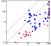
IC3+IA(LRA)		TreeIC3+IA(LRA)
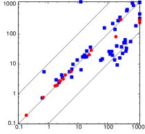
	IC3(LRA)		TreeIC3+ITP(LRA)
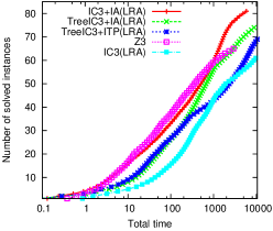
		Algorithm/Tool X # solved Tot time IC3+IA(LRA) 82 5836 TreeIC3+IA(LRA) 75 8825 TreeIC3+ITP(LRA) 70 10478 z3 66 2923 IC3(LRA) 62 9637

Figure 3: Experimental results on LRA benchmarks from [7].

In the first part of our experiments, we evaluate the impact of Implicit Abstraction for the performance of IC3 modulo theories. In order to do so, we compare IC3+IA(LRA) and TreeIC3+IA(LRA) against IC3(LRA) and TreeIC3+ITP(LRA) on the same set of benchmarks used in [7], expressed in the LRA theory. We also compare both variants against the SMT extension of IC3 for LRA presented in [15] and implemented in the z3 SMT solver.

The results are reported in Figure 3. In the scatter plots at the top, safe instances are shown as blue squares, and unsafe ones as red circles. The plot at the bottom reports the number of solved instances and the total accumulated execution time for each tool. From the results, we can clearly see that using abstraction has a very significant positive impact on performance. This is true for both the fully symbolic and the CFG-based IC3, but it is particularly important in the fully symbolic case: not only IC3+IA(LRA) solves 20 more instances than IC3(LRA), but it is also more than one order of magnitude faster in many cases, and there is no instance that IC3(LRA) can solve but IC3+IA(LRA) can’t. In fact, Implicit Abstraction is so effective for these benchmarks that IC3+IA(LRA) outperforms also TreeIC3+IA(LRA), even though IC3(LRA) is significantly less efficient than TreeIC3+ITP(LRA). One of the reasons for the smaller performance gain obtained in the CFG-based algorithm might be that TreeIC3+ITP(LRA) already tries to avoid expensive quantifier elimination operations whenever possible, by populating the frames with clauses extracted from interpolants, and falling back to quantifier elimination only when this fails (see [7] for details). Therefore, in many cases TreeIC3+ITP(LRA) and TreeIC3+IA(LRA) end up computing very similar sets of clauses. However, implicit abstraction still helps significantly in many instances, and there is only one problem that is solved by TreeIC3+ITP(LRA) but not by TreeIC3+IA(LRA). Moreover, both abstraction-based algorithms outperform all the other ones, including z3.

We also tried a traditional CEGAR approach based on explicit predicate abstraction, using a bit-level IC3 as model checking algorithm and the same interpolation procedure of IC3+IA(LRA) for refinement. As we expected, this configuration ran out of time or memory on most of the instances, and was able to solve only 10 of them.

Finally, we did a comparison with a variant of IC3 specific for timed automata, Atmoc [17]. We randomly selected a subset of the properties provided with Atmoc, ignoring the trivial ones (i.e. properties that are 1-step inductive or with a counterexample of length $<3$). In this case, the comparison is still preliminary and it should be extend it with more properties and case studies. The results are reported in Figure 4. IC3+IA(LRA) performs very well also in this case, solving 100 instances in 772 seconds, while Atmoc solved 41 instances in 3953 seconds (z3 and IC3(LRA) solved 100 instances in 1535 seconds and 46 instances in 3347 seconds respectively).

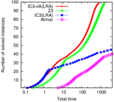
	IC3+IA(LRA)
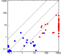
		IC3(LRA)

Figure 4: Preliminary experimental results on timed automata benchmarks.

5.1.1 Impact of number of predicates

The refinement step may introduce more predicates than those actually needed to rule out a spurious counterexample (e.g. the interpolation-based refinement adds all the predicates found in the interpolant). In principle, such redundant predicates might significantly hurt performance. Using the implicit abstraction framework, however, we can easily implement a procedure that identifies and removes (a subset of) redundant predicates after each successful refinement step. Suppose that IC3+IA finds a spurious counterexample trace $\pi=(s_{0},0);\ldots;(s_{k},k)$ with the set of predicates $\mathbb{P}$, and that $\textit{refine}(I,T,\mathbb{P},\pi)$ finds a set $\mathbb{P}_{n}$ of new predicates. The reduction procedure exploits the encoding of the set of paths of the abstract system $S_{\mathbb{P}\cup\mathbb{P}_{n}}$ up to $k$ steps, $\text{BMC}^{k}_{\mathbb{P}\cup\mathbb{P}_{n}}$. If $\mathbb{P}\cup\mathbb{P}_{n}$ are sufficient to rule out the spurious counterexample, $\text{BMC}^{k}_{\mathbb{P}\cup\mathbb{P}_{n}}$ is unsatisfiable. We ask the SMT solver to compute the unsatisfiable core of $\text{BMC}^{k}_{\mathbb{P}\cup\mathbb{P}_{n}}$, and we keep only the predicates of $\mathbb{P}_{n}$ that appear in the unsatisfiable core.

In order to evaluate the effectiveness of this simple approach, we compare two versions of IC3+IA(LRA) with and without the reduction procedure. The results are shown in the scatter plots in Figure 5, both in terms of total number of predicates generated (left) and of execution time (right). Perhaps surprisingly, although the reduction procedure is almost always effective in reducing the total number of predicates , the effects on the execution time are not very big. Although redundancy removal seems to improve performance for the more difficult instances, overall the two versions of IC3+IA(LRA) solve the same number of problems. However, this shows that the algorithm is much less sensitive to the number of predicates added than approaches based on an explicit computation of the abstract transition relation e.g. via All-SMT, which often show also in practice (and not just in theory) an exponential increase in run time with the addition of new predicates. IC3+IA(LRA) manages to solve problems for which it discovers several hundreds of predicates, reaching the peak of 800 predicates and solving most of safe instances with more than a hundred predicates. These numbers are typically way out of reach for explicit abstraction techniques, which blow up with a few dozen predicates.

	Number of predicates		Execution time
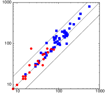
IC3+IA(LRA)		IC3+IA(LRA)
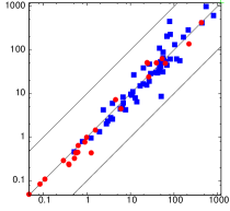
	IC3+IA(LRA) with pred. reduction		IC3+IA(LRA) with pred. reduction

Figure 5: Effects of predicate minimization on IC3+IA(LRA).

5.2 Expressiveness Benefits of Implicit Abstraction

In the second part of our experimental analysis, we evaluate the effectiveness of Implicit Abstraction as a way of applying IC3 to systems that are not supported by the methods of [7], by instantiating IC3+IA(T) (and TreeIC3+IA(T)) over the theories of Linear Integer Arithmetic (LIA) and of fixed-size bit-vectors (BV).

5.2.1 IC3 for BV

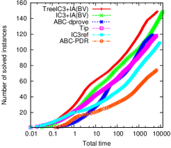
Algorithm/Tool X # solved Tot time TreeIC3+IA(BV) 150 7056 IC3+IA(BV) 150 12753 ABC-dprove 120 4298 Tip 119 6361 IC3ref 110 9041 ABC-pdr 75 6447

Figure 6: Experimental results on BV benchmarks from software verification.

For evaluating the performance of IC3+IA(BV) and TreeIC3+IA(BV), we have collected over 200 benchmark instances from the domain of software verification. More specifically, the benchmark set consists of:

• all the benchmarks used in §5.1, but using BV instead of LRA as background theory;

• the instances of the bitvector set of the Software Verification Competition SV-COMP [2];

• the instances from the test suite of InvGen [12], a subset of which was used also in [24].

We have compared the performance of our tools with various implementations of the Boolean IC3 algorithm, run on the translations of the benchmarks to the bit-level Aiger format: the PDR implementation in the ABC model checker (ABC-pdr) [10], Tip [21], and IC3ref [3], the new implementation of the original IC3 algorithm as described in [5]. Finally, we have also compared with the dprove algorithm of ABC (ABC-dprove), which combines various different techniques for bit-level verification, including IC3. We also tried z3, but it ran out of memory on most instances. It seems that z3 uses a Datalog-based engine for BV, rather than PDR.

The results of the evaluation on BV are reported in Figure 6. As we can see, both IC3+IA(BV) and TreeIC3+IA(BV) outperform the bit-level IC3 implementations. In this case, the CFG-based algorithm performs slightly better than the fully-symbolic one, although they both solve the same number of instances.

5.2.2 IC3 for LIA

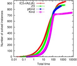
Algorithm/Tool X # solved Tot time IC3+IA(LIA) 933 2064 z3 875 1654 pKind 859 720 Kind 746 8493

Figure 7: Experimental results on LIA benchmarks from Lustre programs [13].

For our experiments on the LIA theory, we have generated benchmarks using the Lustre programs available from the webpage of the Kind model checker for Lustre [13]. Since such programs do not have an explicit CFG, we have only evaluated IC3+IA(LIA), by comparing it with z3 and with the latest versions of Kind as well as its parallel version pKind [16].

The results are summarized in Figure 7. Also in this case, IC3+IA(LIA) outperforms the other systems.

6 Conclusion

In this paper we have presented IC3+IA, a new approach to the verification of infinite state transition systems, based on an extension of IC3 with implicit predicate abstraction.

The distinguishing feature of our technique is that IC3 works in an abstract state space, since the counterexamples to induction and the relative inductive clauses are expressed with the abstraction predicates. This is enabled by the use of implicit abstraction to check (abstract) relative induction. Moreover, the refinement in our procedure is fully incremental, allowing to keep all the clauses found in the previous iterations.

The approach has two key advantages. First, it is very general: the implementations for the theories of LRA, BV, and LIA have been obtained with relatively little effort. Second, it is extremely effective, being able to efficiently deal with large numbers of predicates. Both advantages are confirmed by the experimental results, obtained on a wide set of benchmarks, also in comparison against dedicated verification engines.

In the future, we plan to apply the approach to other theories (e.g. arrays, non-linear arithmetic) investigating other forms of predicate discovery, and to extend the technique to liveness properties.

References

- [1] Barrett, C.W., Sebastiani, R., Seshia, S.A., Tinelli, C.: Satisfiability modulo theories. In: Handbook of Satisfiability, vol. 185, pp. 825–885. IOS Press (2009)
- [2] Beyer, D.: Second Competition on Software Verification - (Summary of SV-COMP 2013). In: Piterman, N., Smolka, S.A. (eds.) TACAS. LNCS, vol. 7795, pp. 594–609. Springer (2013)
- [3] Bradley, A.: IC3ref, https://github.com/arbrad/IC3ref
- [4] Bradley, A., Somenzi, F., Hassan, Z., Zhang, Y.: An incremental approach to model checking progress properties. In: Proc. of FMCAD (2011)
- [5] Bradley, A.R.: SAT-Based Model Checking without Unrolling. In: Proc. of VMCAI. LNCS, vol. 6538, pp. 70–87. Springer (2011)
- [6] Chokler, H., Ivrii, A., Matsliah, A., Moran, S., Nevo, Z.: Incremenatal formal verification of hardware. In: Proc. of FMCAD (2011)
- [7] Cimatti, A., Griggio, A.: Software Model Checking via IC3. In: CAV. pp. 277–293 (2012)
- [8] Cimatti, A., Griggio, A., Schaafsma, B., Sebastiani, R.: The MathSAT5 SMT Solver. In: Piterman, N., Smolka, S. (eds.) Proceedings of TACAS. LNCS, vol. 7795. Springer (2013)
- [9] Clarke, E., Grumberg, O., Long, D.: Model Checking and Abstraction. ACM Trans. Program. Lang. Syst. 16(5), 1512–1542 (1994)
- [10] Een, N., Mishchenko, A., Brayton, R.: Efficient implementation of property-directed reachability. In: Proc. of FMCAD (2011)
- [11] Graf, S., Saïdi, H.: Construction of Abstract State Graphs with PVS. In: CAV. pp. 72–83 (1997)
- [12] Gupta, A., Rybalchenko, A.: Invgen: An efficient invariant generator. In: Bouajjani, A., Maler, O. (eds.) CAV. LNCS, vol. 5643, pp. 634–640. Springer (2009)
- [13] Hagen, G., Tinelli, C.: Scaling Up the Formal Verification of Lustre Programs with SMT-Based Techniques. In: Cimatti, A., Jones, R.B. (eds.) FMCAD. pp. 1–9. IEEE (2008)
- [14] Henzinger, T., Jhala, R., Majumdar, R., McMillan, K.: Abstractions from proofs. In: POPL. pp. 232–244 (2004)
- [15] Hoder, K., Bjørner, N.: Generalized property directed reachability. In: SAT. pp. 157–171 (2012)
- [16] Kahsai, T., Tinelli, C.: Pkind: A parallel k-induction based model checker. In: Barnat, J., Heljanko, K. (eds.) PDMC. EPTCS, vol. 72, pp. 55–62 (2011)
- [17] Kindermann, R., Junttila, T.A., Niemelä, I.: Smt-based induction methods for timed systems. In: Jurdzinski, M., Nickovic, D. (eds.) FORMATS. LNCS, vol. 7595, pp. 171–187. Springer (2012)
- [18] Lahiri, S.K., Nieuwenhuis, R., Oliveras, A.: Smt techniques for fast predicate abstraction. In: CAV. pp. 424–437 (2006)
- [19] McMillan, K.L.: Lazy Abstraction with Interpolants. In: Proc. of CAV. LNCS, vol. 4144, pp. 123–136. Springer (2006)
- [20] Sharygina, N., Tonetta, S., Tsitovich, A.: The synergy of precise and fast abstractions for program verification. In: SAC. pp. 566–573 (2009)
- [21] Sorensson, N., Claessen, K.: Tip, https://github.com/niklasso/tip
- [22] Tonetta, S.: Abstract Model Checking without Computing the Abstraction. In: FM. pp. 89–105 (2009)
- [23] Vizel, Y., Grumberg, O., Shoham, S.: Lazy abstraction and SAT-based reachability in hardware model checking. In: Cabodi, G., Singh, S. (eds.) FMCAD. pp. 173–181. IEEE (2012)
- [24] Welp, T., Kuehlmann, A.: QF_BV model checking with property directed reachability. In: Macii, E. (ed.) DATE. pp. 791–796 (2013)